| Issue |
A&A
Volume 673, May 2023
|
|
|---|---|---|
| Article Number | A1 | |
| Number of page(s) | 21 | |
| Section | Cosmology (including clusters of galaxies) | |
| DOI | https://doi.org/10.1051/0004-6361/202245683 | |
| Published online | 24 April 2023 | |
COVMOS: A new Monte Carlo approach for galaxy clustering analysis
1
Aix Marseille Université, CNRS/IN2P3, CPPM, IPhU, Marseille, France
e-mail: This email address is being protected from spambots. You need JavaScript enabled to view it.
2
Aix Marseille Univ, Université de Toulon, CNRS, CPT, Marseille, France
3
Institute of Space Sciences (ICE, CSIC), Campus UAB, Carrer de Can Magrans, s/n, 08193 Barcelona, Spain
4
Institut d’Estudis Espacials de Catalunya (IEEC), Carrer Gran Capitá 2-4, 08034 Barcelona, Spain
5
Istituto di Astrofisica Spaziale e Fisica cosmica Milano, Via A. Corti 12, 20133 Milano, Italy
Received:
13
December
2022
Accepted:
9
March
2023
Abstract
We validate the COVMOS method introduced in our previous study allowing for the fast simulation of catalogues of different cosmological field tracers (e.g. dark matter particles, halos, galaxies, etc.). The power spectrum and one-point probability distribution function of the underlying tracer’s density field are set as inputs of the method and arbitrarily chosen by the user. To evaluate the validity domain of COVMOS at the level of the produced two-point statistics covariance matrix, we chose to target these two input statistical quantities from realistic N-body simulation outputs. We performed this cloning procedure based on the ΛCDM as well as on a massive neutrino cosmology, for five redshifts in the range of z ∈ [0, 2]. First, we validated the output real-space two-point statistics (both in the configuration and Fourier space) and estimated over 5000 COVMOS realisations per redshift and per cosmology, with a volume of 1 [Gpc/h]3 and 108 particles each. This validation was performed against the corresponding N-body measurements, estimated from 50 simulations. We found the method to be valid up to k ∼ 0.2h Mpc−1 for the power spectrum and down to r ∼ 20 Mpc h−1 for the correlation function. Then, we extended the method by proposing a new modelling of the peculiar velocity distribution, aimed at reproducing the redshift-space distortions both in the linear and mildly non-linear regimes. After validating this prescription, we finally compared and validated the resulting redshift-space two-point statistics covariance matrices in the same range of scales. We released the Python code associated with this method on a public repository, which allows for the production of tens of thousands of realisations in record time. In particular, COVMOS is intended for any study involving large-scale galaxy-survey science that requires a large number of mock realisations.
Key words: large-scale structure of Universe / catalogs
© The Authors 2023
 Open Access article, published by EDP Sciences, under the terms of the Creative Commons Attribution License (https://creativecommons.org/licenses/by/4.0), which permits unrestricted use, distribution, and reproduction in any medium, provided the original work is properly cited.
This article is published in open access under the Subscribe to Open model. This email address is being protected from spambots. You need JavaScript enabled to view it. to support open access publication.
1. Introduction
Understanding the dark sector of the universe constitutes the main challenge of future large galaxy surveys such as Euclid (Laureijs et al. 2011), the Legacy Survey of Space and Time (LSST, LSST Science Collaboration 2009), or the Dark Energy Spectroscopic Instrument (DESI, DESI Collaboration 2016). These surveys have been designed to provide a large amount of data, with the ability to disentangle and constrain several cosmological parameters with a high level of accuracy. Such parameters include the dark energy equation of state and the neutrino mass, as well as more alternative cosmological scenarios, through galaxy clustering, weak lensing, and their cross-correlations.
However, even with infinitely precise and voluminous data, discriminating among different cosmological models is not guaranteed, as it also requires the development of specific analysis methods. The complexity of galaxy survey data analyses mainly relies on the fact that we ought to combine several types of correlated cosmological probes and identify numerous systematic errors and biases. Thus, such analyses must lay on robust statistical tools including a good estimation of correlations in the data and expected error bars. In particular, the cosmological model extraction is based on the evaluation of a likelihood, requiring an accurate covariance matrix for the considered observables (Taylor et al. 2013).
Although predicting the galaxy clustering covariance in a fully analytical way (Wadekar & Scoccimarro 2020; Lacasa 2018; Krause & Eifler 2016) is possible, when one needs to cross-correlate various observables, alternatives to analytical covariances must be developed. As a matter of fact, most of the covariance matrices exploited in galaxy survey analysis today rely on large samples of cosmological simulations (Kitaura et al. 2016; Zhao et al. 2021) and even when an analytical covariance can be used, such as in the recent DES Y3 results (Friedrich et al. 2021), this has to be validated against a covariance sampled from accurate numerical simulations.
In addition to the fact that the construction of such large samples of mock catalogues is highly CPU and time consuming, the major problem is that the covariance is model-dependent: at least one covariance matrix per tested cosmological model is needed (when assuming a covariance matrix constant with respect to the parameters to infer).
Different approaches have been investigated to bypass these issues, called approximate methods. A category of them is designed to speed up the N-body evolution by either approximating the dynamics of the global dark matter field or by focusing on the evolution of early identified halos such as ICE-COLA (Tassev et al. 2013; Izard et al. 2018), PINOCCHIO (Monaco et al. 2002, 2013), or PEAK PATCH (Bond & Myers 1996). Although highly competitive with respect to N-Body simulations (at least up to four-point statistics, see Lippich et al. 2019; Blot et al. 2019; Colavincenzo et al. 2019), they still remain CPU and time-demanding. Other types of methods, such as PATCHY (Kitaura et al. 2013, 2015) or HALOGEN (Avila et al. 2015) are faster than the above methods since they do not require any field evolution. They directly produce the dark matter field at the considered redshift, before applying a biasing scheme (using second order Lagrangian perturbation theory fitted to N-body products to obtain halo catalogues. However, these methods require a certain level of calibration and therefore remain indirectly expensive to adapt from one cosmological model to another.
Finally, a third category of approximate methods has already been studied in the specific case of log-normal density fields (e.g. Coles & Jones 1991; Greiner & Enßlin 2015). These methods consist in targeting, at a given redshift, both the clustering amplitude, usually through the power spectrum, and the probability distribution function (PDF) of the simulated density field. A discretisation of this field, based on the so-called local Poisson process approximation, can eventually be applied to obtain a discrete set of objects. Because of the rapidity and the simplicity of implementation of such methods, a vast amount of literature has investigated the log-normal distributions (e.g. Xavier et al. 2016; Alonso et al. 2014; Agrawal et al. 2017). However, it has been shown by Carron (2011) that the log-normal statistics poorly reproduce the true data correlations when entering the non-linear regime, due to the limited range of validity of such approximated PDF forms (see Tosone et al. 2020, for an extension).
In this context, we introduced in Baratta et al. (2020) a new Monte Carlo method fully suited for simulating catalogues of objects defined by an arbitrary power spectrum and a one-point PDF. In the present work, we aim at validating this method against the DEMNUni (Carbone et al. 2016; Castorina et al. 2015; Parimbelli et al. 2022) set of N-body simulations. We thus evaluate the validity domain of the two-point statistic covariance matrices produced with the COVMOS1 public code.
This paper is organised as follows. In Sect. 2, we detail the core of the method and generalise it to the simulation of power spectra with non-linear prescriptions. In Sect. 3, after introducing the DEMNUniN-body simulations, we compare and discuss the results for the produce two-point statistics (the power spectrum and the two-point correlation function) in real space. We then extend the Monte Carlo method by introducing our peculiar velocity assignment procedure in Sect. 4, describing how we reproduced redshift-space distortions effects both in the linear and mildly non-linear regimes. We compare the auto- and cross-covariances in the redshift space for the multipoles of the anisotropic power spectrum and two-point correlation function with those of the N-body reference in Sect. 5. In Sect. 6 we present our conclusions.
2. Theoretical pipeline in real space
In this section, we recall the basics of the pipeline that enables the generation of a discrete set of objects defined by a given, arbitrary one-point PDF and density power spectrum. For a more detailed description of the method, we refer to Baratta et al. (2020).
In the first stage, we focus on the generation of the continuous density field. Then we discuss how to circumvent the limit of the method, that is, the production of negative, non-physical power spectra, when the target power spectrum is the non-linear one. Finally, we describe how to discretise the field into point-like tracers.
2.1. Targeting a given PDF and power spectrum
The main ingredient of the pipeline lays on the local, non-linear mapping of an initial (centered and reduced) Gaussian field ν(x)≡𝒩(0, 1) such that
![Mathematical equation: $$ \begin{aligned} \delta (x) \equiv {\mathcal{L} } \left[\nu (x)\right], \end{aligned} $$](/articles/aa/full_html/2023/05/aa45683-22/aa45683-22-eq1.gif) (1)
(1)
where the resulting δ-field must represent the final cosmological, non-Gaussian contrast density field. The transformation, ℒ, can be found using standard probability transformation rules, as long as a target δ-PDF is set. In particular, using the local conservation of probabilities between ν and δ, ℒ in Eq. (1) can directly be identified as:
![Mathematical equation: $$ \begin{aligned} \delta = C_\delta ^{-1}[C_\nu (\nu )], \end{aligned} $$](/articles/aa/full_html/2023/05/aa45683-22/aa45683-22-eq2.gif) (2)
(2)
where CY is defined as the cumulative function of the field Y. The results of Eq. (1) not only impact the moments of ν, but also its two-point statistics. By consistently using probability conservation properties, we can quantify the effect of applying a local transformation, ℒ, to the Gaussian field through the mapping, λ, via:
 (3)
(3)
where 𝒫ν(ν1, ν2, ξν) is the bivariate normal distribution of ν, and ξν ≡ <ν1ν2>c its corresponding two-point correlation function. ξδ stands for the two-point correlation function of the cosmological field.
Since the power spectrum, P(k), is the Fourier transform of the two-point correlation function, we can rely on the mapping, λ, in order to predict the input power spectrum of the Gaussian field, ν. Indeed, according to Appendix C of Bel et al. (2016), with |ξν|< 1, λ turns out to be continuous and monotonic in this interval. This implies the existence of the reciprocal function λ−1, ensuring that Eq. (3) is inverted as ξν = λ−1(ξδ).
As a matter of fact, once ξδ is known (provided that Pδ(k) is the target power spectrum), being able to compute ξν is equivalent to finding the power spectrum Pν(k) to be assigned to the initial Gaussian field. This specific field is then generated such that, once transformed under the local mapping, ℒ, the resulting δ-field follows the targeted power spectrum, Pδ(k). Formally speaking, an overview of the pipeline is expressed as:
![Mathematical equation: $$ \begin{aligned} P_\nu (k) = {\mathcal{F} } \left\{ \lambda ^{-1} {\mathcal{F} }^{-1}\left[ P_\delta (k) \right] \right\} \ , \end{aligned} $$](/articles/aa/full_html/2023/05/aa45683-22/aa45683-22-eq4.gif) (4)
(4)
where ℱ and ℱ−1 stand respectively for the Fourier and inverse Fourier transforms of the power spectra. The presented inversion scheme relies on our ability to evaluate the transformation λ of the two-point correlation function. Therefore, we need to numerically compute Eq. (3)2.
2.2. Practical implementation: Constraints and limits
Here, we consider a periodic, cubical comoving volume of a size, L. We assume that the different fields are sampled on a regularly spaced grid in this box, characterised by the sampling parameter Ns, representing the number of grid nodes per dimension. In this setting, we must now consider a three-dimensional description of the various fields and two-point statistics. In particular, the quantities described in Sect. 2.1 become ν(x)→ν(x), δ(x)→δ(x), P(k)→P(k), and so on.
Since generating a non-Gaussian density field in the configuration space requires us to start from an initial Gaussian field in Fourier space3, the Monte Carlo method extensively uses three-dimensional (3D) fast Fourier transforms (FFT) and their inverse (IFFT) in order to be efficient. As a result, we have to sample the generated fields on a regular grid in the configuration space, producing (in the Fourier space) a well known effect called aliasing (Jing 2005). Basically, the FFT of a sampled field is the standard Fourier transform of the field itself, to which replicas (or aliases) of it are added. This produces an extra power on scales close to the Nyquist frequency kN = π/(L/Ns), also affecting the Fourier phases. Assuming that IFFT[FFT[Y]] = Y (or equivalently that the IFFT of an aliased field is the ‘right’ field in the configuration space), the targeted power spectrum, Pδ(k), used in Eq. (4) must be artificially aliased according to4
 (5)
(5)
so that the method may be self-consistent. Here, n ≡ (n1,n2,n3) ∈ ℤ3. Simply stated, the set of fields we generate in Fourier space must necessarily be aliased. This ensures the fields in configuration space to be unaffected by aliasing.
Moreover, as the cosmological fields are sampled on a finite grid, this naturally introduces a smoothing scale of their statistics, related to the quantity L/Ns. As a consequence, prior to the application of Eq. (4), the two statistical inputs (power spectrum and PDF) must be smoothed consistently with the grid. This is natural for the PDF if its targeted shape is directly estimated on the same grid type, as well as for the power spectrum if it remains convolved with the mass assignment scheme (MAS) needed for its estimation through a FFT (Sefusatti et al. 2016). However, in the case of a target power spectrum that is free from any filtering effect (i.e. if the effect of the MAS has been removed from the estimated power spectrum or for a theoretical one), a scan filtering of the power spectrum must be considered in such a way that the variances of the two inputs of the method are matching, prior to the computation of its 3D aliased version (following Eq. (5)). Such a scan filtering can be performed using multiple filtering radius, R1, values in:
![Mathematical equation: $$ \begin{aligned} P^\mathrm{filt}(k) = P(k)F(k) = P(k)\ \mathrm{exp} \left[ -(kR_1)^i \right] \,, \end{aligned} $$](/articles/aa/full_html/2023/05/aa45683-22/aa45683-22-eq6.gif) (6)
(6)
where i is a free parameter weighting the filtering tail shape. For such a low-pass filter, it should be noted that the aliasing contributions are significantly reduced. However, for the sake of accuracy, we still take them into account.
It is worth mentioning that this Monte Carlo procedure is not rigorously implementable with regard to any shape of power spectrum, especially one characterised by a non-linear prescription. This would produce negative values in the 3D power spectrum Pν(k) in Eq. (4), whether aliasing Eq. (5) is taken into account or not. Such an outcome is at this stage not understood. As an example, with a high resolution grid of Ns = 1024 and L = 1000 Mpc h−1, corresponding to a precision of ∼1 Mpc h−1, about ∼45% of negative elements are produced for a ΛCDM non-linear power spectrum at redshift z = 0. They are mainly located in the Fourier volume in the vicinity of the Nyquist frequency. This number of negative values is reduced for Ns = 512 (∼20%) and disappears for Ns = 256. However, choosing such poor grid setting would inevitably reduce the range of usable simulated modes.
On the one hand, the variance,  , estimated from the power spectrum of the Gaussian field (with kF = 2π/L being the fundamental frequency of the periodic box) is actually fully unitary (as required by the procedure), while, on the other hand, these non-physical negative elements prevent the simulation of the Gaussian field,
  . To sidestep this restriction, a corrective method can be adopted: this consists of clipping to zero all negative values. As a direct consequence, the variance computed on the new 3D power spectra automatically deviates from unity with
  . In order to recover the procedure condition,
  , an additional 3D filtering can be applied to match the unit variance. Here, we propose the 3D filtering version of Eq. (6), that is:
![Mathematical equation: $$ \begin{aligned} F({\boldsymbol{k}}) = \mathrm{exp} \left[ -(\boldsymbol{k}R_2)^j \right]\ . \end{aligned} $$](/articles/aa/full_html/2023/05/aa45683-22/aa45683-22-eq11.gif) (7)
(7)
Naturally, this procedure has the effect of reducing the maximum mode up to which the power spectrum is reliably simulated. While R1 and R2 are constrained by the previously discussed conditions on the variance, i and j should be chosen in such a way that the simulated power spectrum matches the targeted one up to a maximum wave-mode. Their values are discussed in Sect. 3.
We go on to briefly summarise the method to provide a global understanding. We generated, in Fourier space, a Gaussian field, ν, on a 3D grid defined by the power spectrum Pν(k) (Eq. (4)), after being corrected using Eq. (7). We then perform an inverse FFT of ν(k) to get ν(x) and locally applied the non-linear transform, ℒ, to it, as in Eq. (1). The obtained field, δ(x), is now expected to both follow the target density PDF (the exact one) and (filtered) power spectrum.
2.3. From continuous field to discrete catalogues
In order to finalise the procedure above, we can turn the obtained density field, δ(x), into a discrete catalogue of objects by applying a local Poisson sampling (Layzer 1956) of it. Provided a mean number density, ρ0, expected in a catalogue of volume, V, and a simulated local density contrast field, δ(x), we can estimate the number of objects, Λ, which is locally expected within a small volume element, a3 = (L/Ns)3, as Λ = ρ0a3(1 + δ).
Of course, this expected number Λ is not an integer. However, it can be seen as the expectation value that we should see if the sampling was made several times at a position x. Thus, the number of observed objects in the small volume, a3, can be drawn from a Poisson distribution with an expectation value Λ.
We can think about two kinds of interpolation schemes when placing the corresponding number of particles within the grid cell. The first is the so-called top hat scheme, where particle coordinates follow a uniform distribution. It is fast, but the density fields will appear structurally discontinuous. A natural extension of this method that is able to fix this issue is the tri-linear scheme, implemented here by populating the grid cell with particles following the tri-linearly interpolated density field distribution. In Appendix A, we detail the method that allows for such assignment of particles in voxels. We note that both methods have an impact on the shape of the resulting Poisson power spectrum, which fortunately can be accurately predicted even beyond the Nyquist frequency (see Baratta et al. 2020).
To anticipate our outcomes, we find that the choice of the interpolation scheme has no impact on the estimated covariance matrix in the considered wave-mode range. Nonetheless, in the following, we only use the three-linear interpolation scheme.
2.4. Discussion
The method can be viewed as a cloning procedure of a power spectrum and a PDF obtained from an original reference catalogue. For the method to be optimal, the ideal choice for the MAS used to estimate the PDF must be compatible with the type of interpolation scheme used to assign coordinates to particles. For example, in the case of the tri-linear interpolation process, a cloud in cell (CIC) MAS should have been used to estimate the PDF. This would allow for a better reproduction of the 1p-PDF at the end of the chain. However, for technical reasons, it is often impossible to estimate this kind of PDF without it being heavily affected by noise. It is therefore generally more convenient to resort to a piecewise cubic spline (PCS) estimated PDF, which is less affected by noise5. COVMOS not proposing the equivalent of the PCS to place particles, the 1-p PDF of the cloned catalogue cannot be expected to be identical to the original reference simulation and will seem over-smoothed. However, such a discrepancy is materialised for scales smaller than the grid size, affecting only the scales beyond our scales of interest.
Moreover, before going through the validation of the pipeline in Sect. 3, it must be mentioned the fact that the clipping procedure of the negative elements of the power spectrum introduced in Eq. (7) has some key statistical consequences. First, there is the fact that the produced mean density,  is not rigorously zero but may systematically be shifted to a level of ∼10−3. This excess of mean density cannot simply be subtracted since it correlates with the associated realised power spectra at all k modes. A non-trivial consequence of this additional correlation is the biasing of the two-point statistics covariances, Appendix B shows in details how this bias can be identified and subtracted. We note that all results involving covariances in the following of this article has been corrected for this bias.
3. Application in real space
The method introduced above allows us to simulate, within a cubical volume, objects whose nature (dark matter particles, dark matter halos, galaxies, etc.) only depends on the choice of the input density power spectrum and PDF. In this section, for simplicity, we simulate dark matter particles in real space when targeting the statistics of a set of N-body simulations. We evaluate the range of reliability of the produced two-point statistics for a reasonable (computationally speaking) grid sampling precision of Ns = 1024.
3.1. DEMNUni_covN-body simulations
Originally developed for testing different probes in the presence of massive neutrinos and dynamical dark energy, the Dark Energy and Massive Neutrino Universe (DEMNUni6; Carbone et al. 2016) experiment is a suite of N-body simulations (Roncarelli et al. 2015; Castorina et al. 2015; Moresco et al. 2017; Fabbian et al. 2018; Zennaro et al. 2018; Ruggeri et al. 2018; Bel et al. 2019; Kreisch et al. 2019; Schuster et al. 2019; Verza et al. 2019, 2022b,a; Parimbelli et al. 2021, 2022; Guidi et al. 2022; Hernández-Molinero et al. 2023) in ΛCDM, plus different νw0waCDM cosmological scenarios. The largest simulations follow the evolution of 20483 CDM and (if present) 20483 neutrino particles, in a box of side L = 2 Gpc h−1. They have been produced on various high-performance computing (HPC) machines provided by the super computing centre CINECA7, Italy, by exploiting the GADGET-3 code of Springel (2005), further developed by Viel et al. (2010) for the inclusion of massive neutrino particles.
All the simulations of the DEMNUni have in common the following cosmological parameters:
The initial conditions have been set at redshift z = 99 using the Zeldovich approximation (Zeldovich 1970) and the public code described in Zennaro et al. (2016, 2018, 2019).
The evolution of cosmic structures is simulated down to redshift z = 0, while outputting 63 particle snapshots with equally spaced logarithmic scale factor intervals. Among these snapshots, we restrict the analysis of this work to the five following redshifts:8

Regarding our study oriented toward the estimation of covariances, only the DEMNUni subset, hereafter called DEMNUni_cov Parimbelli et al. (2021), constitutes the reference basis for the validation tests of our Monte-Carlo method. This subset is made of two ΛCDM cosmologies, one without massive neutrinos and the other one with massive neutrinos (added at the level of massive particles inside the simulation) of a total mass, Mν = 0.16 eV. In the following, these two cosmologies are referred to as ‘ΛCDM’ and ‘16nu’, respectively. The main objective in using these two suites of simulations is that they are run 50 times each with different realisations of the initial conditions. In this way, they offer the possibility of estimating the covariance matrices to some extent.
Each simulation consists of 10243 dark matter particles of mass mp ≃ 8 × 10¹⁰ M⊙ h−1, and 10243 massive neutrino particles (in the case of the massive neutrino cosmology) of a mass  in a cubical volume of size L = 1000 Mpc h−1 with periodic boundary conditions. For each snapshot of each realisation, we estimated the PDF and the power spectrum of the matter field using a PCS MAS on a grid of sampling parameter Ns = 1024. The power spectrum was estimated using the NBodyKit9 (Hand et al. 2018) software, applying the interlacing method to reduce the aliasing (Sefusatti et al. 2016).
The averaged PDF and filtered power spectra (following the prescription in Eq. (6)) of the 50 simulations can then be directly used as targets for the Monte Carlo code. It is to be stressed that the method requires a high level of precision in the estimation of the PDF that is targeted. In practice, we estimate a logarithm-spaced histogram of the δ-field from −1 to the maximal value of δ obtained from a catalogue smoothed on the grid following a defined MAS (δ ∼ 103 in the present case of a PCS on the DEMUNni_cov catalogues). We obtained about 106 values. A bad estimate (in terms of precision) of the PDF leads to a bad computation of the transformation, ℒ, linking the Gaussian field to the non-Gaussian fields (see Eq. (1)) and, as a consequence, the two-point correlation function of the initial Gaussian field that systematically leads to a higher number of negative elements in the power spectrum. However, this can, in practice, be avoided by resorting to a fit of a given analytical PDF. For our purposes, we checked that having 50 simulations was enough to avoid issues with extreme peaks (related to a bad estimate of the tail of the PDF). Finally, in the case where the randomly drawn Gaussian fields hits the 0th percentile in the δ-PDF, nothing pathological can affect the field, typically because the actual probability of finding −1 is zero. On the other hand, for the 100th percentile, this operation would be similar to clipping because a mode cannot supperate the maximum density contrast seen in the 50 DEMUNni_cov simulations.
3.2. Comparing the two-point statistics
In the first place, for the Monte Carlo simulations to be run, we must fix the values of the filtering parameters i and j (see Eqs. (6) and (7)). For various combinations of them, with i taking several intermediate values in [2, 6] and j in [2, 10], we can predict the output Pδ(k) of the method by explicitly computing FFT[λ(ξν)] (see Eq. (3)). We can shell average the resulting 3D power spectra in shells of width kF and compare them to the targeted one. The results, presented in Fig. 1, show that, in order to maximise the range of well simulated modes, i must be equal to 3 for redshifts z = [0, 0.5], then i = 4 for z = [1, 1.5] and, finally, i = 5 for z = 2. On the other hand, an arbitrarily large value for j can be chosen. Figure 1 only presents the results for the ΛCDM scenario. We note that in the present case, as well as for the following figures, only one cosmology will be discussed if the same results are obtained also for the other one.
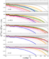 |
Fig. 1. Relative deviation between the predicted grid power spectrum (after the two filterings Eq. (6) and (7)) and the corresponding target power spectrum for all five selected redshifts in the ΛCDM cosmology (similar results are obtained for the massive neutrinos, 16nu cosmology). The predicted spectra are computed for all combinations of parameters i = [2, 3, 4, 5, 6] and j = [2, 4, 6, 8, 10]. Each colour represents a certain value of i, respectively blue, orange, green, red, and violet. An increasing colour intensity means an increasing j value. The dotted black line is the relative deviation when only the first filter, Eq. (6), is applied, taking the identified optimal i, respectively 3, 3, 4, 4, and 5. The grey area delimits the 1% limit. |
Moreover, from this figure, we can see the successive effects of the two filtering, Eqs. (6) and (7). The difference between the dotted black line and zero is due to the first filter. We recall that this smoothing is exclusively due to the fact that the fields are set on a finite grid. The difference between the dotted black line and the coloured ones shows the impact of the second filter, required to solve issue of the negative elements of the spectrum.
For the present analysis, in the following, we use the same doublet parameters (i, j) for all redshifts and cosmologies, fixing them to (i = 2.5, j = 8). This choice was first motivated by the fact that we want to carry out a comparative study of the method between the redshifts, without adding extra tuning to enhance the output statistics (i.e. maximising the range of validity of the produced power spectra). Second, we recall that the PDF is obtained from a PCS MAS. This has the particularity of acting as a filter on the power spectrum fairly well reproduced by Eq. (6), with i = 2.5. Given such a choice, we try to keep a good consistency between these two statistics. Moreover, since we can’t anticipate an eventual effect of a doublet (i, j) on the produced covariances, we chose for it to be the same no matter the redshift, to ease the interpretation of the various output statistics.
We ran 5000 simulations of COVMOS catalogues per redshift in the ΛCDM and 16nu cosmologies. Each of them consists of 108 dark matter particles in boxes of size L = 1000 Mpc h−1. We recall that the target statistics of the method are the ones estimated on the DEMNUni_cov simulations.
After removing the relatively low shot noise contribution to the estimated power spectra (PSN ∼ 0.04h−3Mpc3), we compare them to the ones estimated from the DEMNUni_cov in Fig. 2. As expected, we can observe a smaller range of reliable simulated wave modes when compared to its grid equivalent in Fig. 1. Indeed, as already discussed, the Poisson sampling gives rise to a smoothing of the cosmic field that visually starts to dominate around k ∼ 0.2 h Mpc−1. This smoothing has the direct consequence to reduce the maximum accurately simulated Fourier mode to around k ∼ 0.25 h Mpc−1 (in the 1-σ limit). We recall that this result is obtained assuming a grid precision of Ns = 1024. Improving this setting would lower the effect of the smoothing induced by the applied assignment schemes. However, because of these negative spectrum problems to be corrected, it can be expected that the method (whatever the grid accuracy employed) may be limited to a minimum scale. It is also noted that this filtering effect is similar, regardless of the redshift. This is due to the fact that we have defined the parameters i and j as constants.
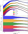 |
Fig. 2. Real space power spectrum comparison between the COVMOS and the DEMNUni_cov experiments. Top panel: estimated and averaged real space power spectrum monopoles over 5000 realisations of COVMOS catalogues in 16nu cosmology, with dispersion on each realisation represented in colour. The same quantities are represented in black for the 50 DEMNUni_cov realisations. Bottom panels: relative deviations between the averaged COVMOS and DEMNUni_cov measurements in dashed black lines with error bars following the same colour-coding. |
When switching to the configuration space, we estimated the two-point correlation functions over the 50 DEMNUni_cov realisations at z = 0 and for the 16nu cosmology only. The outputs were compared to a set of 100 correlation functions estimated on the COVMOS set of simulations. We restricted this number given the high computational cost of estimating such statistics. Figure 3 shows this comparison in the range of scales [0.1, 125] Mpc h−1, depicting a high level of agreement between the two methods for all scales higher than 7 Mpc h−1. Below this limit, correlations seem to be over-produced in the range of [1.5, 5] Mpc h−1 and under-produced for scales of < 1.5 Mpc h−1.
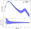 |
Fig. 3. Real-space two-point correlation function comparison between the COVMOS and the DEMNUni_cov experiments. Top: estimated and averaged correlation function monopoles over 100 realisations of COVMOS catalogues in 16nu cosmology at z = 0, with dispersion on each realisation represented in blue. The solid black line represents the averaged power spectra (with dispersion over measurements in dashed black lines) over 50 DEMNUni_cov simulations. Bottom: residual between the COVMOS and DEMNUni_cov outputs, with error bars. |
4. Theoretical pipeline in the redshift space
In galaxy surveys, the observed positions of tracers of the matter field are systematically affected by their peculiar velocities. As a consequence, the power spectrum is affected at all scales, this is the so-called redshift-space distortion (RSD) effect. Indeed, it acquires an angular dependence with respect to the line of sight, losing the property of being isotropic. The amplitude of its angular average is enhanced in the linear regime due to the coherent in-fall of objects toward high density regions; this is the so-called Kaiser effect (Kaiser 1987). In the non-linear regime (on smaller scales), the density fluctuations and velocities are coupled in a non trivial way (Scoccimarro 2004) which make the RSD effects on the power spectrum difficult to be predicted accurately.
In the present section, we show our practical implementation of peculiar velocities in the COVMOS code. The main idea is to first generate a velocity field correlated with the density field so that we make sure that we are able to reproduce the Kaiser effect on large scale.
In principle, applying the Monte Carlo pipeline (as detailed in Sect. 2) to generate a continuous velocity field (as long as a corresponding power spectrum and a PDF are provided) is perfectly feasible. However, several subtle points must be addressed. The first is related to the fact that we expect the divergence of the peculiar velocity field, vp, and the density field, δ, to be correlated to satisfy the linear continuity equation:
 (8)
(8)
where f is the growth rate of structures. This implies that the velocity field cannot be simulated in an independent way from the density field, δ.
Beside, once the velocity field has been generated on a regular grid in space, we need to carefully associate a velocity to the previously generated tracers anywhere in the simulated volume. In the following, we detail these two main steps in order to simulate a catalogue of objects together with their peculiar velocities.
4.1. Simulating the velocity field
The method that we developed to generate the velocity field is based on the fact that when estimating the velocity field with a Delaunay tesselation in DEMNUni simulations (as in Bel et al. 2019), the PDF of each velocity component appears to be close to Gaussian (see the black dashed line in Fig. 5, as compared to the Gaussian model in red dashed). In addition, we want to reproduce the power spectrum of the divergence of the velocity field and, finally, as stated before, we need to satisfy the continuity equation.
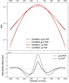 |
Fig. 5. Comparison of the one-point and smoothed PDFs estimated from the COVMOS and DEMNUni_cov experiments. Top: estimated one-point (solid lines) and smoothed (dashed lines) velocity PDF from one COVMOS simulation in red and one DEMNUni_cov simulation in black. The smoothed velocity PDF is estimated from a Delaunay tesselation of the particle coordinates of the DEMNUni_cov_01 experiment. This map is then interpolated on a grid of sampling parameter Ns = 512. Here the cosmology is ΛCDM. Bottom: residual between the DEMNUni_cov and COVMOS PDF. |
Let us define the scaled velocity field u(x) as:
 (9)
(9)
where E(z)≡H(z)/H0, such that the observed comoving distance, s, of an object can be deduced from the true one r as s = r − ur (ur being the line of sight projection of u). The idea is then to generate the divergence, θ(x)=∇ ⋅ u, of the scaled velocity field in Fourier space according to the power spectrum of the divergence of the velocity field and to assume that the velocity field, u, is curl-free:
 (10)
(10)
This way it is only necessary to generate the divergence, θk, in Fourier space with a real and an imaginary part following a centred Gaussian distribution with a variance given by the power spectrum of the divergence Pθθ(k). We note, however, that in order to satisfy to the continuity equation, we impose the condition that the Gaussian field, ν, used to generate the density field is also used to generate the divergence. This means that we impose strictly the continuity equation only in the linear regime. To do so, we can rely on the fitting functions given in Bel et al. (2019):
 (11)
(11)
 (12)
(12)
where  stands for the linear cold dark matter plus baryons power spectrum (numerically predicted by Boltzmann codes) and
 (13)
(13)
 (14)
(14)
 (15)
(15)
where σ8, m is the rms of the linear matter fluctuations smoothed on spheres of radius 8 Mpc h−1 and must be predicted for the total matter (accounting for massive neutrinos).
In summary, we start by simulating, on a Fourier grid, the Gaussian θ-field using the same random Fourier phases as for the density field, defined by the non-linear θ − θ power spectrum in Eq. (12). This field is then converted in the 3-dimensional velocity field in Eq. (10), which we apply an inverse Fourier transform to so that we can obtain the velocity field in configuration space, u(x), taken from Eq. (9).
4.2. Drawing peculiar velocities
In order to properly reproduce redshift-space distortions, it is necessary to assign velocities to the objects inside the simulated catalogue. To this aim we could interpolate the regularly spaced velocity grid u(x) at all the positions of the objects, however, this would not accurately reproduce the non-linear redshift space distortions. Indeed, on small scales, we would expect that the angular average power spectrum is suppressed by the fact that inside halos, the velocities are not coherent; instead, they are close to be random thanks to the virial theorem. That is the reason why we drew the velocity of each object out of a Gaussian distribution centred on the interpolated value of the velocity field, u, at the position of the object and with a given dispersion, Σ. This is a similar method to the one used by de la Torre & Peacock (2013) in order to assign velocities to halos below the mass resolution of a simulation.
Aimed at being as realistic as possible, we allow the velocity dispersion to depend on the underlying matter density. In fact, we would expect that more massive halos have a large velocity dispersion (Elahi et al. 2018). Using the DEMNUni_cov simulations, we estimated the relation between the local density 1 + δ and the velocity variance  . By fixing the grid sampling to Ns = 1024, we can run an estimation of the local velocity variance as a function of the local density contrast value over the 50 simulations in the two cosmologies, ΛCDM and 16nu, for the five redshifts z = [0,0.5,1,1.5,2]. This is represented in Fig. 4 where (in the upper panel) we show that no matter what the considered redshift, there is a clear relation between the velocity dispersion and the density. Indeed, this relation exhibits a very low level of stochasticity, meaning that we can further assume there is an analytical relation between the local dispersion and the density. In addition, the lower panel of Fig. 4 shows that the presence of massive neutrinos induces changes in this relationship. As expected, the dispersion in a cosmology with massless neutrinos is systematically higher.
 |
Fig. 4. Velocity variance as a function of the local density estimated on the DEMNUni_cov simulations. Top: combined velocity components variance in (km/s)2 as a function of local density contrast for the DEMNUni_cov set of 50 simulations and for the five redshifts z = [0, 0.5, 1, 1.5, 2] in the case of the standard ΛCDM cosmology. Bottom: percent relative deviation, redshift per redshift, between the two cosmologies, ΛCDM and 16nu, still using the same colour-code. |
When inspecting Fig. 4, we can see that the global behaviour of the velocity dispersion-density relation can be approximated as a power law. Even if this does not seem to be accurate for low values of the density, we further assume a power law relationship. This is justified for two reasons. First when the density is low, so is the dispersion. Thus, the way we model the relation is expected to affect less the final velocities of the various objects in the catalogues. Second, when the density is low, we estimate both the density and the velocity dispersion with a low number of objects, thus the shot noise can introduce a bias. Thus, in the end, we adopt the following analytical form
 (16)
(16)
where α is fixed from the velocity dispersion-density relation estimated from DEMNUni_cov and listed in the right column of Table 1. The second parameter, β, is not taken from the simulations, but it needs to be set in order to make sure that the one-point velocity dispersion σV of the catalogues is matching the one of DEMNUni_cov (this will be explained more in details in the following).
Averaged one-point velocity rms (in Mpc/h) of the one-point velocity distribution as measured from particles from the 50 DEMNUni_cov simulations, per redshift and per cosmology.
We note also that the exponent α of the power law can be related to dynamics inside over-densities and thus (by extension) inside halos. In fact, we checked that if one uses halos to estimate the velocity dispersion-density relation, then the same value for α is measured but with a different normalisation β.
The measured one-point velocity variances are listed in the left column of Table 1, where we can see that it decreases with the redshift and that adding massive neutrinos is reducing it. As anticipated, we fix the normalisation β so that the one-point velocity variance,  , is the same as the one-point velocity variance measured in the DEMNUni_cov catalogues.
Furthermore, matching the one-point velocity variance allows us to provide a physical description of the amplitude parameter, β. Thus, we can show how the one-point variance is related to the prescription in Eq. (16) when going from the large scale velocity to the velocity of individual objects. Indeed, the peculiar velocity, Vp, assigned to a particle, can be formally expressed as
 (17)
(17)
where w = −aHu and v is drawn from an uncorrelated tri-variate centred reduced Gaussian distribution. This means that the conditional probability distribution, 𝒫(Vc|wc, ρ), of a single component, Vc, of the vector, Vp, is given by:
 (18)
(18)
Since we define the variance of a single velocity component as the arithmetic mean of the square of the velocity component, it turns out that:
 (19)
(19)
due to the fact that the density of points is not uniformly distributed, thus, regions with higher density will provide a larger contribution to the expectation value.
From Eq. (19), in order to predict the one-point velocity variance,  , we need to express the one-point probability distribution of the object velocity component, Vc, which depends on the density and the velocity, wc, as
 (20)
(20)
Substituting Eqs. (18) and (20) in the expression in Eq. (19) and using the fact that the second-order moment of the Gaussian distribution is reduce to the sum of its variance and the squared of its expectation value, Eq. (19) is simplified to:
![Mathematical equation: $$ \begin{aligned} \sigma _V^2 = \int \int \mathrm{d}{ w}_c \mathrm{d}\rho \ {\mathcal{P} }({ w}_c,\rho )\rho \left[ { w}_c^2 + \Sigma ^2(\rho )\right] = \sigma _{ w}^2 + \sigma ^2_\Sigma \ . \end{aligned} $$](/articles/aa/full_html/2023/05/aa45683-22/aa45683-22-eq33.gif) (21)
(21)
In the above expression the first term,  , is the variance of the interpolated velocity field that can be estimated independently from the choice of the function Σ2(ρ), while this is not the case for the second marginalised term, defined as
  . Then, coming back to our simple model in Eq. (16), the β parameter can be obtained using Eq. (21) as:
 (22)
(22)
where  is directly estimated on the interpolated density field at the object coordinates.
In Fig. 5, we compare the distribution of the velocity components of the regularly sampled velocity field w, estimated from the DEMNUni_cov, with the same distribution obtained from COVMOS. We see that the Gaussian approximation assumed to generate the velocity field is indeed a good approximation. In addition, we compare the one-point velocity PDF estimated from a COVMOS realisation of (exceptionally) ∼109 dark matter particles with the one estimated from particles in a DEMNUni_cov realisation. We can see that, assuming a power law relation between the velocity dispersion and the matter density (Eq. (16)) and fixing the normalisation of the relation by requiring that the one-point velocity dispersion of COVMOS matches the one of DEMNUni_cov (Eq. (22)), allowing us to reproduce the non-Gaussian distribution of the particle velocity. Indeed, by matching only the second order cumulant moment, we can also reproduce the exponential tails of the distribution. In the next section, we show the efficiency of our approximations for generating the velocity field at the level of the power spectrum in the redshift space.
5. Applications in the redshift space
In this section, we describe how we applied the whole pipeline for simulating particles (described in Sect. 2) and their associated peculiar velocities (Sect. 4). We study to which extent the various two-point statistics, associated error bars and correlations are reliably simulated.
5.1. Validating the two-point statistics
With the same settings applied in Sect. 3, we simulated 5000 catalogues of 108 dark matter particles with associated peculiar velocities, for all five redshifts and for the two cosmologies. We estimate on each realisation the multipoles of the power spectrum:
 (23)
(23)
where ℒℓ(x) are defined as the Legendre polynomials on the order of ℓ, μk ≡ cos(ϕk) and ϕk is the angle between the line of sight and the wave vector, k. We adopt the plane parallel limit which consists in choosing the line of sight as being a fixed direction in the simulated co-moving volume.
Generating the entire set of simulations and measuring their associated real- and redshift-space power spectra took nearly 20 days, running on about 940 processors of 2.4 GHz. We note that reducing the precision of the COVMOS grids to Ns = 512, three days are necessary to simulate and estimate the power spectrum of 100 000 catalogues.
In Figs. 6 and 7, we compare the power spectra of COVMOS to those estimated in the reference DEMNUni_cov, N-body simulations. An initial observation of Fig. 6 leads us to the very same conclusions as those drawn for its real-space equivalent Fig. 2. The ratios  in both spaces do indeed seem similar. The maximal wave-mode at which the power spectra are reliably simulated are conserved. We can, however, note a gain in power of the redshift-space power spectrum at z = 0, with respect to its real-space equivalent. Such effects can be due to an overestimation of the β parameter in Eq. (22), which, in our code implementation, is averaged over a tens of realisations before becoming constant for the whole set of simulations. To correct for this effect, the beta parameter should be obtained from a larger number of realisations. Our new version of COVMOS averages 100 values for β, estimated on single realisations.
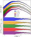 |
Fig. 6. Redshift-space power spectrum comparison between the COVMOS and the DEMNUni_cov experiments. Top panel: average of the estimated redshift-space power spectrum monopoles over 5000 realisations of COVMOS catalogues in the 16nu cosmology. The dispersion on each realisation is represented by the shaded area. The same quantities are represented in black for the 50 DEMNUni_cov realisations. Bottom panels: relative deviation between the averaged COVMOS and DEMNUni_cov outputs in dashed black lines with error bars following the same colour-coding. |
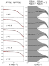 |
Fig. 7. Comparison of the redshift-space to real space power spectrum monopoles ratio between the COVMOS and DEMNUni_cov experiments. Left: ratio between averaged monopoles with and without RSD contribution in black for DEMNUni_cov and in red for COVMOS, for the five different redshifts. Right: Ratio between the previous quantities in black solid line with error bars in shaded grey, jointly accounting for estimated variance on DEMNUni_cov and COVMOS in both real and redshift-space. |
In order to quantify the robustness of the proposed velocity model, we can see the redshift-space to real-space averaged monopole ratio in Fig. 7. In the left panels, we can see that the effects of RSD on the power spectrum are well reproduced in COVMOS when compared to DEMNUni_cov. For both the enhancement of the apparent clustering in the linear regime (≤0.1h Mpc−1) or its suppression in the mildly non-linear regime (≥0.1h Mpc−1), the velocity model allows us to reproduce (with high fidelity) the large-scale limit (Kaiser boost) as well as the transition to smaller scales.
Finally, looking at the ratio between the previous quantity in the COVMOS and DEMNUni_cov cases allows us to extract and discuss the validity domain of the proposed velocity modelling (right panel of Fig. 7). While the model seems to perfectly recover the RSD effects in the linear regime at the percent level, a gradual departure can be observed in the non-linear regime. We observe a lack of power for k ≥ 0.6 h Mpc−1, which can be due to the severe filtering of the COVMOS fields in this regime. Since we cannot expect the peculiar velocity assignment method to be adapted to a highly suppressed clustering amplitude, the grid precision here seems to be ill-suited with regard to validating the velocity model on highly non-linear scales (k ≥ 0.6 h Mpc−1).
For completeness, in Fig. 8, we compare the higher order multipoles of the power spectrum between COVMOS and DEMNUni_cov. As in the case of the monopole, in the linear regime, both the amplitude and the dispersion of the simulated multipoles are in good agreement. In addition, it appears that in the mildly non-linear regime, these multipoles are not impacted by the various filterings affecting the monopoles (see Fig. 6). Indeed, none of these multipoles show a clear lack of power for k > 0.2 h Mpc−1, so that this anisotropic part of the power spectrum turns out to be reliably simulated on a wider range than the redshift-space monopole.
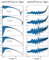 |
Fig. 8. Comparison of the redshift-space power spectrum multipoles between the COVMOS and DEMNUni_cov experiments: absolute values of the averaged quadrupoles (left panels) and averaged hexadecapoles (right panels) for the DEMNUni_cov in solid black lines (error bars in dashed black lines) and for COVMOS with error bars in blue for the five redshifts. |
As in real space, we can also make a comparison in redshift-space at the level of the two-point correlation function. We ran the estimation of the configuration space correlation function multipoles (applying periodic boundary conditions) over a smaller sample of 100 COVMOS realisations, in the 16nu cosmology only at z = 0. In addition, we estimated the two-point correlation functions on the complete set of 50 DEMNUni_cov simulations. Figure 9 displays the averaged monopole, quadrupole, and hexadecapole, compared between COVMOS and DEMNUni_cov on the scale range of r ∈ [0, 125] Mpc h−1. We can see that the redshift space multipoles produced by COVMOS are in agreement with what is expected from DEMNUni_cov at least down to 40 Mpc h−1. Indeed, in that regime, it is not only the amplitude that is matching, but also the dispersion of the measurements. We can also notice that despite the fact that we made this verification at redshift z = 0, the monopole is well reproduced on even smaller scales (∼20 h−1Mpc) than the other multipoles. This serves as a validation of our scheme to assign velocities in configuration space as well.
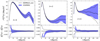 |
Fig. 9. Redshift-space two-point correlation function multipoles comparison between the COVMOS and the DEMNUni_cov experiments. Top: average of the estimated two-point correlation function multipoles over 100 realisations of COVMOS catalogues in 16nu cosmology, at z = 0 with dispersion on each realisation represented in blue. The solid black line represents the same (with dispersion over measurements in dashed black lines) for DEMNUni_cov simulations. Bottom: residual between the averaged COVMOS and DEMNUni_cov multipoles with corresponding error bars. |
5.2. Comparing the real and redshift-space covariance matrices
In this section we compare the covariance matrices produced by the two methods, obtained from the standard estimator:
![Mathematical equation: $$ \begin{aligned} \hat{C}_{ij}&= \frac{1}{N-1}\sum _{s=1}^{N} [P^s(k_i)-\mu _i][P^s(k_j)-\mu _j]\ , \\ \mu _i&=\frac{1}{N}\sum _{s=1}^{N} P^s(k_i) \nonumber \ , \end{aligned} $$](/articles/aa/full_html/2023/05/aa45683-22/aa45683-22-eq40.gif) (24)
(24)
where Ps(ki) is the power spectrum of the s-th simulation (over a total of N) evaluated at mode ki.
The statistics, according to Scoccimarro et al. (1999), can be decomposed into two terms:
 (25)
(25)
referred to as the Gaussian and non-Gaussian contributions, respectively. The former is related to the amplitude of the power spectrum, normalised by the number of independent averaged modes Mki within shells centred around ki, only affecting the diagonal of the matrix. The second affects the whole matrix and depends on the cross shell-averaged trispectrum:
 (26)
(26)
where the trispectrum can be constructed from the density field as
 (27)
(27)
Expected to be zero in the case of a Gaussian realisation, this second contribution directly weighs the non-Gaussian nature of the simulated cosmic fields.
While the first term (in the case of the COVMOS method) is expected to be suppressed when the various filterings start to act (k > 0.2h Mpc−1 for a grid precision of Ns = 1024), the second term is not so obvious to assume. The main approximation of COVMOS is to suppose that  can be (to some extent) properly reconstructed if both the power spectrum and the PDF are accurate. However, such a connection remains difficult to foresee. In any case, this term is expected to dominate the non-linear regime and to become raised in power as the targeted PDF follows a more clustered, skewed shape.
With regard to the estimator of the covariance, Eq. (24) will be associated in the following an analytical error-bar, which is predicted when assuming a Gaussian multivariate distribution of the data (Wishart 1928):
![Mathematical equation: $$ \begin{aligned} V\left[ \hat{C}_{ij}\right] = \frac{C_{ij}^2+C_{ii}C_{jj}}{N-1}\ . \end{aligned} $$](/articles/aa/full_html/2023/05/aa45683-22/aa45683-22-eq45.gif) (28)
(28)
In Fig. 10, we show the contributions to the variance, both in the DEMNUni_cov and the COVMOS cases, for all redshifts and in the 16nu cosmology. The figure shows that for the five redshifts, the full variances,  , are matching within Gaussian error bars. This observation can also be extended to modes well beyond those for which the power spectrum is correctly reproduced. This effect can be understood when decomposing the variance in Gaussian and non-Gaussian contributions (Eq. (25)): the former is computed from the average power spectrum over the realisations, whereas the latter is obtained by subtracting the Gaussian contribution from the total variance. In doing so, we can see that in the linear regime, the Gaussian term that dominates the second term (by about one order of magnitude) unsurprisingly follows the same trend as discussed for the power spectrum. It is accurately reproduced, but starts to disagree with the N-body reference around k = 0.2h Mpc−1. On the other hand, as the damping happens at scales where the trispectrum term starts to dominate, it allows us to recover this lack of power and produces an overall variance with correct amplitude. Nevertheless, we can observe at z = 0, a systematic overestimate of this term, from k ∼ 0.25h Mpc−1 both in the real and redshift space. This could be due to the insufficiency of our approximations at very low redshift.
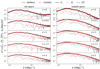 |
Fig. 10. Comparison of the real and redshift-space power spectrum covariance matrices (the diagonal part) between the COVMOS and DEMNUni_cov experiments. Estimated contributions of the diagonal of the covariance matrices over 5000 realisations of COVMOS catalogues (in red) in real (left) and redshift-space (right) as compared to the ones estimated from 50 DEMNUni_cov (in black) for the five redshifts and in 16nu cosmology. The estimated diagonals |


We compare all terms of the covariance matrices obtained for the N-body and the COVMOS method for the three redshifts z = [0, 1, 2] in Figs. 11–13, respectively. This comparison is conducted in real-space for the monopole and in the redshift space for all multipoles, where we also show the cross-covariances between multipoles. We represent the residual of the COVMOS and DEMNUni_cov matrices in standard deviation, namely:
 (29)
(29)
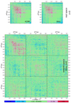 |
Fig. 11. Difference in σ-deviation between the cross-covariance matrices of the power spectrum in Fourier space obtained from 5000 COVMOS and 50 DEMNUni_cov realisations at z = 0. This difference is normalised by the predicted Gaussian error in Eq. (28); also see Eq. (29). Upper panels show the monopoles in real space for the two cosmologies, while the bottom panels stand for the cross-covariance terms in the redshift space, for the 16nu cosmology only. |
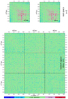 |
Fig. 12. Difference in σ-deviation between the cross-covariance matrices of the power spectrum in Fourier space obtained from 5000 COVMOS and 50 DEMNUni_cov realisations at z = 1. This difference is normalised by the predicted Gaussian error in Eq. (28); also see Eq. (29). Upper panels give the monopoles in real space for the two cosmologies, while the bottom panels stand for the cross-covariance terms in the redshift space, for the 16nu cosmology only. |
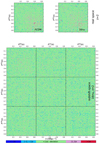 |
Fig. 13. Difference in σ-deviation between the cross-covariance matrices of the power spectrum in Fourier space obtained from 5000 COVMOS and 50 DEMNUni_cov realisations at z = 2. This difference is normalised by the predicted Gaussian error Eq. (28), see Eq. (29). in Eq. (28); also see Eq. (29). Upper panels give the monopoles in real space for the two cosmologies, while the bottom panels stand for the cross-covariance terms in the redshift space, for the 16nu cosmology only. |
where the  terms are computed using Eq. (28). Looking at these three figures, we can first remark a large number of over- or under-estimations of the covariance terms – without any apparent global trend. They constitute the only observable feature that we can see in redshift space at z = 1 and z = 2 and in real space at z = 2. This is explained by the stochastic noise, unrelated to the validity of the method, expected to follow a centered and reduced normal distribution. Thus, drawing the distribution of Rij against its prediction helps in the discusson of the validity of the produced covariances. To avoid overloading the figures, this is shown only at z = 0 in Fig. 14, taking a maximal mode kmax = 0.25h Mpc−1. In this regime in the redshift space, we can see that the measured distribution is in good agreement with the prediction, demonstrating that no bias in the COVMOS matrices can be detected. This is not as strong in the real space, where we can detect a shift of the distribution toward larger σ values. This depicts an overall over-estimation of the covariance elements that can be easily spotted in the top panels of Fig. 11.
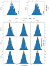 |
Fig. 14. Normalised distributions of the residual of the covariance matrices normalised by Gaussian error (the σ-deviation distribution, see Fig. 11) for the multipoles of the power spectrum at z = 0 in blue. Its Gaussian fit (on the two first moments) is represented in black and is compared to the standardised normal distribution in orange. Upper panels presents the distributions in real space for the two cosmologies, while the bottom panels give the results in the redshift space, for the 16nu cosmology only. In these panels, the maximal Fourier mode is set to kmax = 0.25h Mpc−1. |
Secondly, we can see in real space a migration of an over-correlation pattern toward higher scales for decreasing redshift. These over-correlations are maximised around the diagonal at z = 0 from k ∼ 0.2h Mpc−1 to k ∼ 0.5h Mpc−1 and no change can be noticed when switching from one cosmology to another. Once again, this can be attributed to the weak validity of the COVMOS approximations at low redshift z ∼ 0.
On the other hand, it turns out that the redshift-space covariance terms are systematically better simulated than their equivalents in real space. This effect is more apparent at z = 0 where the systematic over-estimate of the correlations in real space are significantly reduced in the redshift space. This improvement is in agreement with Fig. 10, showing a slight increase of the range of reliability of the trispectrum in redshift than in real space. According to Eq. (25), the off-diagonal terms of the covariance matrix are only related to the trispectrum terms, explaining why the whole matrices in the redshift space are more accurate than in real-space. Further investigation is required to determine why the trispectrum is better simulated in the redshift space as compared to real space. It is evident that the presented method cannot reproduce the full trispectrum in real space, thus limiting us in that regard. However, in the redshift space, the velocity field features contribute to a significant portion of the trispectrum shape, and the proposed method might perform better due to the relationship between the density and local velocity dispersion.
Concerning the other multipoles and their cross-covariance terms in the redshift space, no particular over or under-correlation pattern throughout the simulated redshifts can be observed beyond the noise, as depicted in Fig. 14. At these probed redshifts, both error bars and correlations of the multipoles are in good agreement with the N-body outputs.
Finally, Figs. 15 and 16 show the results for the variance and the covariance of the two-point correlation function multipoles, respectively, both in the real and the redshift spaces.
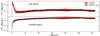 |
Fig. 15. Comparison of the real and the redshift space of the two-point correlation function covariance matrices (the diagonal part) between the COVMOS and DEMNUni_cov experiments. Estimated diagonal of the two-point correlation function covariance matrix in real (top panel) and redshift space (bottom panel) estimated from 50 DEMNUni_cov realisations in black and 100 COVMOS realisations in red. Assuming a Gaussian distribution of the data, errors bars are computed from Eq. (28). |
Focusing on real space, the variance of the two-point correlation function monopole seems to be reproduced in a reliable way down to ∼6 Mpc h−1, before being successively over- (2 < r < 6 Mpc h−1) and under- (r < 2 Mpc h−1) estimated, which is in agreement with the observation made directly on the two-point correlation function monopole in Fig. 9. These observations can also be made for the whole monopole covariance in the upper panel of Fig. 16: a majority of the matrix elements fall in the < |1σ| deviation (> 68%) in the regime > ∼ 6 Mpc h−1 before getting over- or under-estimated above this limit.
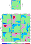 |
Fig. 16. Difference in σ-deviation between the covariance matrices of the multipoles of the two-point correlation function estimated from 100 COVMOS realisations and 50 DEMNUni_cov realisations. This difference is normalised by the predicted Gaussian errors estimated from Eq. (28). The upper panel stands from the comparison of the monopole in real space, while the bottom panels stands for the covariance terms of the multipoles in the redshift space. |
In the redshift space, as for the power spectrum analysis, a significant improvement in the simulation of the errors and correlations are observed on small scales. The variance of the monopole is now reliable down to ∼3 Mpc h−1, while the under-estimation of the correlation between scales (observed in the real space) is damped in this case. Despite the fact that we have a less significant number of realisations in the case of the two-point correlation function, we can see that in general the covariance and cross-covariance of the two-point correlation multipoles is well reproduced. More realisations would be needed to assess the significance of the 2-sigma deviations around 30 Mpc h−1 in the cross-covariance between the monopole and the quadrupole and in the covariance of the quadrupole. Indeed, we started with 50 realisations only and so, generating 50 more greatly improved the comparison.
6. Conclusion and discussion
Although it is apparently straightforward, the reliance on covariance matrices for two-point statistics estimators evaluated from mock catalogues generally leads to two main issues. The first is the sampling noise that propagates down to the parameter constraints and turns out to be difficult to correct without making any assumption on the posterior distribution of parameters (Gouyou Beauchamps et al. in prep., Dodelson & Schneider 2013; Percival et al. 2014; Taylor et al. 2013; Taylor & Joachimi 2014). The second (and less investigated) concern is the computational cost of evaluating a covariance matrix for various set of cosmological parameters in order to study potential biases due to the fiducial choice of the cosmology when analysing data.
In this context, we propose a method implemented in the public code named COVMOS, allowing the fast production of a large number of catalogues. Each individual catalogue is a realisation of a non-Gaussian density field, characterised by a probability density function and a power spectrum. In Baratta et al. (2020), we showed that it is possible to reproduce with a high level of accuracy a given PDF and a power spectrum, but it is limited to real space and to a log-normal PDF. In the present paper, we present two major improvements :
-
the probability distribution function of the density field can be arbitrarily set as an input; this way, we can mimic the PDF measured from a N-body simulation or provide a theoretical model.
-
we designed a peculiar velocity assignment procedure that accurately models the effect of redshift-space distortion on two-point statistics at least up to k = 0.5h Mpc−1.
As a result, it is necessary to specify a set of statistical quantities and relations as inputs of the code. These are used as targets for the pipeline. These include: (i) the power spectra of the density and (ii) velocity fields, (iii) the one-point probability distribution function of the density field, and (iv) a relation between the velocity dispersion and the density.
In addition, we validated the whole COVMOS pipeline in the real and redshift spaces, for two-point statistics (the power spectrum and the correlation function) and their associated covariance matrices, against state-of-the art N-body simulations (DEMNUni). We investigated the performance of two cosmological models: a standard ΛCDM model and one including massive neutrinos. In both cosmological scenarios, we show that for a spatial resolution of the order of 1h−1Mpc, in a comoving volume of 1h−3Gpc, the matter power spectrum multipoles in the redshift space are reliably reproduced up to k = 0.25 h Mpc−1 (down to r = 10h−1Mpc for the two-point correlation function).
We extended the validation of the method to 4-point statistics in Fourier space. More precisely, we verified that the shell-averaged trispectrum,  , which enters the power spectrum covariance, is in good agreement with the one obtained from 50 N-body simulations. This results in an accurate reproduction of the power spectrum covariance matrices. Although it is slightly over-estimated in real space for k ∼ 0.15 h Mpc−1, it turns out that in the redshift space, we can reach k ∼ 0.2 h Mpc−1 for the monopole power spectrum.
Having validated the method against N-body simulation, a major advantage of the code is its numerical efficiency in terms of computational cost. As an example, for this work, we generated 5 × 5000 catalogues of 108 objects in 20 days on a HPC cluster10, using 940 processors of 2.4 GHz. Thus, we were able to generate an extremely large number (25k) of realisations in less than 20k cpu-hr, in order to produce noise-free covariance matrices. Indeed, it is faster to generate a realisation than to estimate the power spectrum of that realisation, and the difference is even more important when considering the estimation of the two-point correlation function.
The method may need to be further investigated to reach a higher level of precision and accuracy before a potential application in the final data analysis of large galaxy surveys. We note that the precision of the method is governed by two factors. The first is the grid precision set by the user that has to have the effect of smoothing the statistics at a certain scales. The second constraint is less controllable. It is related to the production of negative elements in some of the pipeline power spectra. A scale limitation is therefore to be expected and would require further inspection to be carefully determined. However, the associated public code can already be useful for a broad variety of applications. Indeed, its ability to simulate a wide variety of cosmological models and to achieve almost no sampling noise in the produced covariance matrices makes this method particularly relevant for testing likelihood pipelines (see Gouyou Beauchamps et al. in prep., for a first application) aimed at constraining cosmological parameters.
Finally, we recall that the COVMOS code is public11, fully written in Python, ready to be used and adapted to receive the needed inputs either from theory or simulations. This is a method specialised in producing two-point statistics and associated by-products (covariance matrices) that may produces unrealistic outputs when considering other statistics. In particular the method does not account for structure formation physics, and is not capable of producing a cosmic web with the richness of collapsed structures (e.g. clusters, filaments and voids). It is therefore not advisable to use statistics beyond those presented in this study.
A natural extension of this method, which would bring it closer to the results of observations, would be the reconstruction of the observed light-cone that is aimed at accounting, for instance, for survey window function effects. In addition, this would allow for the production of angular maps, suited for the study of photometric statistics in the Spherical Harmonics domain. Given it is a method specialised in two-point statistics, correlated maps of observables such as galaxy clustering and galaxy shear could be produced, as well as their associated cross-covariances. Future extensions could also include radio observations such as CMB temperature maps, CMB-lensing, or even 21-cm maps. Given the improvement in their performance that the exploitation of cross-correlations between different observables will provide to ongoing and future cosmological surveys – especially for parameter degeneracy breaking through their combinations – the COVMOS method and its further developments will certainly prove useful in modern cosmology.
Publicly available in https://github.com/PhilippeBaratta/COVMOS
It can be shown that it is possible to switch the 2D integral of Eq. (3) into a sum of finite 1D integrals, quickly converging and therefore less computationally expensive. As a result, computing the Hermite expansion of the local mapping, ℒ, allows us to write down the Taylor expansion of the two-point correlation function, ξν. For more details, we refer to Appendix C of Bel et al. (2016).
Generating a Gaussian field with a given power spectrum is greatly simplified in the Fourier space.
We consider here an aliasing correction in the context of a nearest grid point (NGP) window; see Sefusatti et al. (2016).
Note that a the target power spectrum smoothed using i = 2.5 in Eq. (6) matches the PCS window.
http://www.cineca.it/
For simplification in the following, these five redshifts will be referred to the round numbers z = {0, 0.5, 1, 1.5, 2}.
https://nbodykit.readthedocs.io/en/latest/
The Dark Energy Cluster (DEC) hosted in CPPM, Marseille.
https://github.com/PhilippeBaratta/COVMOS
Note: there is no uniqueness in the method.
Acknowledgments
PB and SGB were supported by CNES, focused on Euclid mission. The project leading to this publication has received funding from Excellence Initiative of Aix-Marseille University -A*MIDEX, a French “Investissements d’Avenir” programme (AMX-19-IET-008 -IPhU). The DEMNUni simulations were carried out in the framework of “The Dark Energy and Massive-Neutrino Universe” project, using the Tier-0 IBM BG/Q Fermi machine and the Tier-0 Intel OmniPath Cluster Marconi-A1 of the Centro Interuniversitario del Nord-Est per il Calcolo Elettronico (CINECA). We acknowledge a generous CPU and storage allocation by the Italian Super-Computing Resource Allocation (ISCRA) as well as from the coordination of the “Accordo Quadro MoU per lo svolgimento di attività congiunta di ricerca Nuove frontiere in Astrofisica: HPC e Data Exploration di nuova generazione”, together with storage from INFN-CNAF and INAF-IA2.
References
- Agrawal, A., Makiya, R., Chiang, C.-T., et al. 2017, JCAP, 10, 003 [CrossRef] [Google Scholar]
- Alonso, D., Ferreira, P. G., & Santos, M. G. 2014, MNRAS, 444, 3183 [NASA ADS] [CrossRef] [Google Scholar]
- Avila, S., Murray, S. G., Knebe, A., et al. 2015, MNRAS, 450, 1856 [NASA ADS] [CrossRef] [Google Scholar]
- Baratta, P., Bel, J., Plaszczynski, S., & Ealet, A. 2020, A&A, 633, A26 [NASA ADS] [CrossRef] [EDP Sciences] [Google Scholar]
- Bel, J., Branchini, E., Di Porto, C., et al. 2016, A&A, 588, A51 [NASA ADS] [CrossRef] [EDP Sciences] [Google Scholar]
- Bel, J., Pezzotta, A., Carbone, C., Sefusatti, E., & Guzzo, L. 2019, A&A, 622, A109 [NASA ADS] [CrossRef] [EDP Sciences] [Google Scholar]
- Blot, L., Crocce, M., Sefusatti, E., et al. 2019, MNRAS, 485, 2806 [NASA ADS] [CrossRef] [Google Scholar]
- Bond, J. R., & Myers, S. T. 1996, ApJS, 103, 1 [NASA ADS] [CrossRef] [Google Scholar]
- Carbone, C., Petkova, M., & Dolag, K. 2016, J. Cosmol. Astro-Part. Phys., 2016, 034 [CrossRef] [Google Scholar]
- Carron, J. 2011, ApJ, 738, 86 [NASA ADS] [CrossRef] [Google Scholar]
- Castorina, E., Carbone, C., Bel, J., Sefusatti, E., & Dolag, K. 2015, JCAP, 07, 043 [CrossRef] [Google Scholar]
- Colavincenzo, M., Sefusatti, E., Monaco, P., et al. 2019, MNRAS, 482, 4883 [NASA ADS] [CrossRef] [Google Scholar]
- Coles, P., & Jones, B. 1991, MNRAS, 248, 1 [NASA ADS] [CrossRef] [Google Scholar]
- de la Torre, S., & Peacock, J. A. 2013, MNRAS, 435, 743 [CrossRef] [Google Scholar]
- DESI Collaboration (Aghamousa, A., et al.) 2016, arXiv e-prints [arXiv:1611.00036] [Google Scholar]
- Devroye, L. 1986, Non-Uniform Random Variate Generation (Springer-Verlag) [CrossRef] [Google Scholar]
- Dodelson, S., & Schneider, M. D. 2013, Phys. Rev. D, 88, 063537 [Google Scholar]
- Elahi, P. J., Power, C., Lagos, C. d. P., Poulton, R., & Robotham, A. S. G. 2018, MNRAS, 477, 616 [NASA ADS] [CrossRef] [Google Scholar]
- Fabbian, G., Calabrese, M., & Carbone, C. 2018, J Cosmol. Astropart. Phys., 2018, 050 [CrossRef] [Google Scholar]
- Friedrich, O., Andrade-Oliveira, F., Camacho, H., et al. 2021, MNRAS, 508, 3125 [NASA ADS] [CrossRef] [Google Scholar]
- Greiner, M., & Enßlin, T. A. 2015, A&A, 574, A86 [NASA ADS] [CrossRef] [EDP Sciences] [Google Scholar]
- Guidi, M., Veropalumbo, A., Branchini, E., Eggemeier, A., & Carbone, C. 2022, ArXiv e-prints [arXiv:2212.07382] [Google Scholar]
- Hand, N., Feng, Y., Beutler, F., et al. 2018, AJ, 156, 160 [Google Scholar]
- Hernández-Molinero, B., Carbone, C., Jimenez, R., & Peña Garay, C. 2023, ArXiv e-prints [arXiv:2301.12430] [Google Scholar]
- Izard, A., Fosalba, P., & Crocce, M. 2018, MNRAS, 473, 3051 [NASA ADS] [CrossRef] [Google Scholar]
- Jing, Y. P. 2005, ApJ, 620, 559 [NASA ADS] [CrossRef] [Google Scholar]
- Kaiser, N. 1987, MNRAS, 227, 1 [Google Scholar]
- Kitaura, F.-S., Yepes, G., & Prada, F. 2013, MNRAS, 439, L21 [Google Scholar]
- Kitaura, F.-S., Gil-Marín, H., Scóccola, C. G., et al. 2015, MNRAS, 450, 1836 [NASA ADS] [CrossRef] [Google Scholar]
- Kitaura, F.-S., Rodríguez-Torres, S., Chuang, C.-H., et al. 2016, MNRAS, 456, 4156 [NASA ADS] [CrossRef] [Google Scholar]
- Krause, E., & Eifler, T. 2016, MNRAS, 470, 2100 [Google Scholar]
- Kreisch, C. D., Pisani, A., Carbone, C., et al. 2019, MNRAS, 488, 4413 [NASA ADS] [CrossRef] [Google Scholar]
- Lacasa, F. 2018, A&A, 615, A1 [NASA ADS] [CrossRef] [EDP Sciences] [Google Scholar]
- Laureijs, R., Amiaux, J., Arduini, S., et al. 2011, ArXiv e-prints [arXiv:1110.3193] [Google Scholar]
- Layzer, D. 1956, AJ, 61, 383 [NASA ADS] [CrossRef] [Google Scholar]
- Lippich, M., Sánchez, A. G., Colavincenzo, M., et al. 2019, MNRAS, 482, 1786 [NASA ADS] [CrossRef] [Google Scholar]
- LSST Science Collaboration (Abell, P. A., et al.) 2009, ArXiv e-prints [arXiv:0912.0201] [Google Scholar]
- Monaco, P., Theuns, T., & Taffoni, G. 2002, MNRAS, 331, 587 [Google Scholar]
- Monaco, P., Sefusatti, E., Borgani, S., et al. 2013, MNRAS, 433, 2389 [NASA ADS] [CrossRef] [Google Scholar]
- Moresco, M., Marulli, F., Moscardini, L., et al. 2017, A&A, 604, A133 [NASA ADS] [CrossRef] [EDP Sciences] [Google Scholar]
- Parimbelli, G., Anselmi, S., Viel, M., et al. 2021, J. Cosmol. Astropart. Phys., 2021, 009 [CrossRef] [Google Scholar]
- Parimbelli, G., Carbone, C., Bel, J., et al. 2022, J. Cosmol. Astropart Phys., 2022, 041 [CrossRef] [Google Scholar]
- Percival, W. J., Ross, A. J., Sanchez, A. G., et al. 2014, MNRAS, 439, 2531 [NASA ADS] [CrossRef] [Google Scholar]
- Roncarelli, M., Carbone, C., & Moscardini, L. 2015, MNRAS, 447, 1761 [NASA ADS] [CrossRef] [Google Scholar]
- Ruggeri, R., Castorina, E., Carbone, C., & Sefusatti, E. 2018, J Cosmol. Astropart. Phys., 2018, 003 [CrossRef] [Google Scholar]
- Schuster, N., Hamaus, N., Pisani, A., et al. 2019, J Cosmol. Astropart Phys., 2019, 055 [CrossRef] [Google Scholar]
- Scoccimarro, R. 2004, Phys. Rev. D, 70, 083007 [Google Scholar]
- Scoccimarro, R., Zaldarriaga, M., & Hui, L. 1999, ApJ, 527, 1 [NASA ADS] [CrossRef] [Google Scholar]
- Sefusatti, E., Crocce, M., Scoccimarro, R., & Couchman, H. 2016, MNRAS, 460, 3624 [NASA ADS] [CrossRef] [Google Scholar]
- Springel, V. 2005, MNRAS, 364, 1105 [Google Scholar]
- Tassev, S., Zaldarriaga, M., & Eisenstein, D. J. 2013, J. Cosmol. Astropart. Phys., 2013, 036 [CrossRef] [Google Scholar]
- Taylor, A., & Joachimi, B. 2014, MNRAS, 442, 2728 [Google Scholar]
- Taylor, A., Joachimi, B., & Kitching, T. 2013, MNRAS, 432, 1928 [Google Scholar]
- Tosone, F., Neyrinck, M. C., Granett, B. R., Guzzo, L., & Vittorio, N. 2020, MNRAS, 498, 2663 [NASA ADS] [CrossRef] [Google Scholar]
- Verza, G., Pisani, A., Carbone, C., Hamaus, N., & Guzzo, L. 2019, J. Cosmol. Astropart Phys., 2019, 040 [CrossRef] [Google Scholar]
- Verza, G., Carbone, C., Pisani, A., & Renzi, A. 2022a, ArXiv e-prints [arXiv:2212.09740] [Google Scholar]
- Verza, G., Carbone, C., & Renzi, A. 2022b, ApJ, 940, L16 [NASA ADS] [CrossRef] [Google Scholar]
- Viel, M., Haehnelt, M. G., & Springel, V. 2010, JCAP, 06, 015 [CrossRef] [Google Scholar]
- Wadekar, D., & Scoccimarro, R. 2020, Phys. Rev. D, 102, 123517 [NASA ADS] [CrossRef] [Google Scholar]
- Wishart, J. 1928, Biometrika, 20A, 32 [CrossRef] [Google Scholar]
- Xavier, H. S., Abdalla, F. B., & Joachimi, B. 2016, MNRAS, 459, 3693 [NASA ADS] [CrossRef] [Google Scholar]
- Zeldovich, Y. B. 1970, A&A, 5, 84 [Google Scholar]
- Zennaro, M., Bel, J., Villaescusa-Navarro, F., et al. 2016, MNRAS, 466, 3244 [Google Scholar]
- Zennaro, M., Bel, J., Dossett, J., Carbone, C., & Guzzo, L. 2018, MNRAS, 477, 491 [NASA ADS] [CrossRef] [Google Scholar]
- Zennaro, M., Angulo, R. E., Aricò, G., Contreras, S., & Pellejero-Ibáñez, M. 2019, MNRAS, 489, 5938 [NASA ADS] [CrossRef] [Google Scholar]
- Zhao, C., Chuang, C.-H., Bautista, J., et al. 2021, MNRAS, 503, 1149 [CrossRef] [Google Scholar]
Appendix A: Tri-linear assignment
In this appendix, we derive the relations that allow us to populate particles in a cell following a tri-linear interpolation scheme. The cubic volume symbolising a given voxel in tri-linear interpolation is, by construction:
 (A.1)
(A.1)
where ρijk represents the eight local density values defining the vertices of the cube, replacing (i, j, k) by 0 or a = L/Ns. The coordinates x, y and z are defined in the interval [0, a]. Converting it into normalised probability, the 3D PDF is defined as:
 (A.2)
(A.2)
Equation A.2 shows that the three coordinates cannot be generated independently, leading to consider conditional probabilities.
More specifically, the method of sampling a set of points in the cube will use the so-called classical inverse-transform sampling method (Devroye 1986). It relies on the notion of cumulative distribution function (CDF) to generate random numbers from any 1D probability distribution function P(z) in the definition ensemble [a1, a2], defined by:
=\int _{a_1}^z\mathrm{d} z^{\prime }P(z^{\prime })\ . \end{aligned} $$](/articles/aa/full_html/2023/05/aa45683-22/aa45683-22-eq55.gif) (A.3)
(A.3)
Then we have to solve analytically for z using the relation g = CDF[P](z), calling this inversion z = F(g). Finally, given F, a uniform number g in [0, 1] follows P(z).
The different steps for the coordinates assignation are as follows12:
-
Integrate Pρ(x, y, z) over z; z then y; z then x; y then x gives respectively the marginalised probabilities
 ,
,  ,
,  ,
, 
-
Generating Ncell pseudo-random numbers according to the inverse transform sampling method described above for
 completes the coordinates x.
 -
Since
 , where y|x means the conditional probability of y given x, a number Ncell of y-pseudo-random-coordinates depending on the previous ones, x can be generated following
-
In the same way, as
 , Ncell new random numbers targeting
  allows the z-coordinates to be simulated.
Each marginalised probability calculated in point 1 takes the following forms :
 (A.4)
(A.4)
 (A.5)
(A.5)
 (A.6)
(A.6)
where
 (A.7)
(A.7)
The transformations on g in order to successively obtain x, y and z are given by:
![Mathematical equation: $$ \begin{aligned} x&= aC_2^{-1}\left[-C_1+\sqrt{C_1^2+C_2C_3g}\right]\ , \end{aligned} $$](/articles/aa/full_html/2023/05/aa45683-22/aa45683-22-eq69.gif) (A.8)
(A.8)
![Mathematical equation: $$ \begin{aligned} y&= -(2D_1)^{-1}\left[D_2-\sqrt{D_2^2+4gD_1D_3}\right]\ , \end{aligned} $$](/articles/aa/full_html/2023/05/aa45683-22/aa45683-22-eq70.gif) (A.9)
(A.9)
![Mathematical equation: $$ \begin{aligned} z&= -(2E_1)^{-1}\left[E_2-\sqrt{E_2^2+4gE_1E_3}\right], \end{aligned} $$](/articles/aa/full_html/2023/05/aa45683-22/aa45683-22-eq71.gif) (A.10)
(A.10)
with
![Mathematical equation: $$ \begin{aligned} \begin{aligned} C_1&=\rho _{000}+\rho _{0a0}+\rho _{00a}+\rho _{0aa}\\ C_2&=-\rho _{000}+\rho _{a00}-\rho _{0a0}-\rho _{00a}+\rho _{a0a}-\rho _{0aa}+\rho _{aa0}+\rho _{aaa}\\ C_3&=\rho _{000}+\rho _{a00}+\rho _{0a0}+\rho _{00a}+\rho _{a0a}+\rho _{0aa}+\rho _{aa0}+\rho _{aaa}\\ D_1&=a(-\rho _{000}-\rho _{00a}+\rho _{0a0}+\rho _{0aa})\\&\qquad +x(\rho _{000}+\rho _{00a}-\rho _{0a0}-\rho _{0aa}-\rho _{a00}-\rho _{a0a}+\rho _{aa0}+\rho _{aaa})\\ D_2&=2a^2 (\rho _{000}+\rho _{00a})-2ax(\rho _{000}+\rho _{00a}-\rho _{a00}-\rho _{a0a})\\ D_3&=a^2[a(\rho _{000}+\rho _{00a}+\rho _{0a0}+\rho _{0aa})\\&\qquad +x(-\rho _{000}-\rho _{00a}-\rho _{0a0}-\rho _{0aa}+\rho _{a00}+\rho _{a0a}+\rho _{aa0}+\rho _{aaa})]\\ E_1&=a[a(-\rho _{000}+\rho _{00a})+x(\rho _{000}-\rho _{00a}-\rho _{a00}+\rho _{a0a})+\\ &\qquad +y(\rho _{000}-\rho _{00a}-\rho _{0a0}+\rho _{0aa})]+\\&\qquad +xy(-\rho _{000}+\rho _{00a}+\rho _{0a0}-\rho _{0aa}+\rho _{a00}-\rho _{a0a}-\rho _{aa0}+\rho _{aaa})\\ E_2&=2a[a(a\rho _{000}+x(-\rho _{000}+\rho _{a00})+y(-\rho _{000}+\rho _{0a0}))+\\ &\qquad + xy(\rho _{000}-\rho _{0a0}-\rho _{a00}+\rho _{aa0})]\\ E_3&=a^2[a^2(\rho _{000}+\rho _{00a})+a(y(-\rho _{000}-\rho _{00a}+\rho _{0a0}+\rho _{0aa})\\&\qquad +x(-\rho _{000}-\rho _{00a}+\rho _{a00}+\rho _{a0a})) \\&\qquad + xy(\rho _{000}+\rho _{00a}-\rho _{0a0}-\rho _{0aa}-\rho _{a00}-\rho _{a0a}+\rho _{aa0}+\rho _{aaa})].\\ \end{aligned} \end{aligned} $$](/articles/aa/full_html/2023/05/aa45683-22/aa45683-22-eq72.gif) (A.11)
(A.11)
Appendix B: Debiasing the Monte Carlo covariance matrices
The clipping procedure of the negatives elements of the power spectrum, Pν(k), (see Sect. 2.2) inevitably produces a bias in the estimated covariances if they are blindly obtained using Eq. 24. Indeed, in doing so without caution, we would have to conclude that the covariance matrix obtained from COVMOS is systematically over-estimated. This is a spurious effect due to the fact that the k = 0 mode of the non-Gaussian density field obtained from the pipeline, related to ⟨δ⟩, is not rigorously null.
The reason for such a difference comes from the fact that the DC mode, Pν(k = 0), when applying the pipeline represented by Eq. 4, is likely to be negative while we impose it to be null in order to make sure that the Gaussian field has a zero mean (the whole process relies on this assumption). This produces an undesired non-null k = 0 mode in the power spectrum of the density field, δ, which introduces a correlation between the volume averaged density,  with the power spectrum at all k modes. Thus, the power spectrum at different wave mode being correlated with a hidden variable (
 ), the covariance appears larger than expected. In this appendix, we describe this effect in detail and propose a correction.
A Monte Carlo realisation following the presented pipeline in Sect. 2 will be characterised by a finite total number of object X, which will vary from a realisation to an other. In principle, the variance should be given by the Poisson distribution as  , where Np ≡ ⟨X⟩ is the expectation value of the number of objects in the catalogues. Thus, the expectation value of the number of objects can be obtain by multiplying the volume L3 by the expected number density ρ0: Np = ρ0L3.
When computing the cross-correlation, CXPk ≡ ⟨(X−Np)(P(k)−⟨P(k)⟩)⟩, between the number of object and the amplitude of the power spectrum at a given wave mode, k, we can show that it is given by:
 (B.1)
(B.1)
In Eq. B.1,  stands for the shell average bi-spectrum, a quantity that is, in principle, expected to be null when taken at any k1 or k2 being 0. This is given by the fact that the mean number density is supposed to be known; thus, the mean density contrast is by definition zero and no power appears at any wave-modes k = 0.
As anticipated, if a negative value appears at the k = 0 mode, then it is enforced to be zero. It results in the k = 0 mode of the density power spectrum being expected to be larger than 0. The first effect of this is to provide an extra variance to the Poisson one, such that  .
.
The second effect is to induce a non-negligible shell average bi-spectrum  . Indeed, at leading order, we can express
  with respect to the Hermite coefficients, c1 and c2, that are formally defined in Baratta et al. (2020). This shows that an extra correlation is introduced between the total number of object (or the mean density) and the power spectrum. After having tried to predict precisely the correlation coefficient (using the Mehler expansion of the bi-spectrum) in order to remove it from the computed covariance, we found that the following empirical formula works well and allows us to efficiently recover the correct the covariance:
![Mathematical equation: $$ \begin{aligned} P_{\rm deb}(k) = \left[\frac{N_{p}}{X}\right]^3(\hat{P}(k)-P_{\rm SN}), \end{aligned} $$](/articles/aa/full_html/2023/05/aa45683-22/aa45683-22-eq81.gif) (B.2)
(B.2)
where PSN = (1/(2π))/ρ0 is the shot noise contribution to the power spectrum. The overall correction is just taking into account that the global effect of having more or less particles is to resize the amplitude of the power spectrum. At the end of the day, the shot noise corrected power spectrum that will be used for covariance matrix estimation will therefore be Pdeb(k).
All Tables
Averaged one-point velocity rms (in Mpc/h) of the one-point velocity distribution as measured from particles from the 50 DEMNUni_cov simulations, per redshift and per cosmology.
All Figures
|
Fig. 1. Relative deviation between the predicted grid power spectrum (after the two filterings Eq. (6) and (7)) and the corresponding target power spectrum for all five selected redshifts in the ΛCDM cosmology (similar results are obtained for the massive neutrinos, 16nu cosmology). The predicted spectra are computed for all combinations of parameters i = [2, 3, 4, 5, 6] and j = [2, 4, 6, 8, 10]. Each colour represents a certain value of i, respectively blue, orange, green, red, and violet. An increasing colour intensity means an increasing j value. The dotted black line is the relative deviation when only the first filter, Eq. (6), is applied, taking the identified optimal i, respectively 3, 3, 4, 4, and 5. The grey area delimits the 1% limit. |
| In the text | |
|
Fig. 2. Real space power spectrum comparison between the COVMOS and the DEMNUni_cov experiments. Top panel: estimated and averaged real space power spectrum monopoles over 5000 realisations of COVMOS catalogues in 16nu cosmology, with dispersion on each realisation represented in colour. The same quantities are represented in black for the 50 DEMNUni_cov realisations. Bottom panels: relative deviations between the averaged COVMOS and DEMNUni_cov measurements in dashed black lines with error bars following the same colour-coding. |
| In the text | |
|
Fig. 3. Real-space two-point correlation function comparison between the COVMOS and the DEMNUni_cov experiments. Top: estimated and averaged correlation function monopoles over 100 realisations of COVMOS catalogues in 16nu cosmology at z = 0, with dispersion on each realisation represented in blue. The solid black line represents the averaged power spectra (with dispersion over measurements in dashed black lines) over 50 DEMNUni_cov simulations. Bottom: residual between the COVMOS and DEMNUni_cov outputs, with error bars. |
| In the text | |
|
Fig. 5. Comparison of the one-point and smoothed PDFs estimated from the COVMOS and DEMNUni_cov experiments. Top: estimated one-point (solid lines) and smoothed (dashed lines) velocity PDF from one COVMOS simulation in red and one DEMNUni_cov simulation in black. The smoothed velocity PDF is estimated from a Delaunay tesselation of the particle coordinates of the DEMNUni_cov_01 experiment. This map is then interpolated on a grid of sampling parameter Ns = 512. Here the cosmology is ΛCDM. Bottom: residual between the DEMNUni_cov and COVMOS PDF. |
| In the text | |
|
Fig. 4. Velocity variance as a function of the local density estimated on the DEMNUni_cov simulations. Top: combined velocity components variance in (km/s)2 as a function of local density contrast for the DEMNUni_cov set of 50 simulations and for the five redshifts z = [0, 0.5, 1, 1.5, 2] in the case of the standard ΛCDM cosmology. Bottom: percent relative deviation, redshift per redshift, between the two cosmologies, ΛCDM and 16nu, still using the same colour-code. |
| In the text | |
|
Fig. 6. Redshift-space power spectrum comparison between the COVMOS and the DEMNUni_cov experiments. Top panel: average of the estimated redshift-space power spectrum monopoles over 5000 realisations of COVMOS catalogues in the 16nu cosmology. The dispersion on each realisation is represented by the shaded area. The same quantities are represented in black for the 50 DEMNUni_cov realisations. Bottom panels: relative deviation between the averaged COVMOS and DEMNUni_cov outputs in dashed black lines with error bars following the same colour-coding. |
| In the text | |
|
Fig. 7. Comparison of the redshift-space to real space power spectrum monopoles ratio between the COVMOS and DEMNUni_cov experiments. Left: ratio between averaged monopoles with and without RSD contribution in black for DEMNUni_cov and in red for COVMOS, for the five different redshifts. Right: Ratio between the previous quantities in black solid line with error bars in shaded grey, jointly accounting for estimated variance on DEMNUni_cov and COVMOS in both real and redshift-space. |
| In the text | |
|
Fig. 8. Comparison of the redshift-space power spectrum multipoles between the COVMOS and DEMNUni_cov experiments: absolute values of the averaged quadrupoles (left panels) and averaged hexadecapoles (right panels) for the DEMNUni_cov in solid black lines (error bars in dashed black lines) and for COVMOS with error bars in blue for the five redshifts. |
| In the text | |
|
Fig. 9. Redshift-space two-point correlation function multipoles comparison between the COVMOS and the DEMNUni_cov experiments. Top: average of the estimated two-point correlation function multipoles over 100 realisations of COVMOS catalogues in 16nu cosmology, at z = 0 with dispersion on each realisation represented in blue. The solid black line represents the same (with dispersion over measurements in dashed black lines) for DEMNUni_cov simulations. Bottom: residual between the averaged COVMOS and DEMNUni_cov multipoles with corresponding error bars. |
| In the text | |
|
Fig. 10. Comparison of the real and redshift-space power spectrum covariance matrices (the diagonal part) between the COVMOS and DEMNUni_cov experiments. Estimated contributions of the diagonal of the covariance matrices over 5000 realisations of COVMOS catalogues (in red) in real (left) and redshift-space (right) as compared to the ones estimated from 50 DEMNUni_cov (in black) for the five redshifts and in 16nu cosmology. The estimated diagonals |
| In the text | |
|
Fig. 11. Difference in σ-deviation between the cross-covariance matrices of the power spectrum in Fourier space obtained from 5000 COVMOS and 50 DEMNUni_cov realisations at z = 0. This difference is normalised by the predicted Gaussian error in Eq. (28); also see Eq. (29). Upper panels show the monopoles in real space for the two cosmologies, while the bottom panels stand for the cross-covariance terms in the redshift space, for the 16nu cosmology only. |
| In the text | |
|
Fig. 12. Difference in σ-deviation between the cross-covariance matrices of the power spectrum in Fourier space obtained from 5000 COVMOS and 50 DEMNUni_cov realisations at z = 1. This difference is normalised by the predicted Gaussian error in Eq. (28); also see Eq. (29). Upper panels give the monopoles in real space for the two cosmologies, while the bottom panels stand for the cross-covariance terms in the redshift space, for the 16nu cosmology only. |
| In the text | |
|
Fig. 13. Difference in σ-deviation between the cross-covariance matrices of the power spectrum in Fourier space obtained from 5000 COVMOS and 50 DEMNUni_cov realisations at z = 2. This difference is normalised by the predicted Gaussian error Eq. (28), see Eq. (29). in Eq. (28); also see Eq. (29). Upper panels give the monopoles in real space for the two cosmologies, while the bottom panels stand for the cross-covariance terms in the redshift space, for the 16nu cosmology only. |
| In the text | |
|
Fig. 14. Normalised distributions of the residual of the covariance matrices normalised by Gaussian error (the σ-deviation distribution, see Fig. 11) for the multipoles of the power spectrum at z = 0 in blue. Its Gaussian fit (on the two first moments) is represented in black and is compared to the standardised normal distribution in orange. Upper panels presents the distributions in real space for the two cosmologies, while the bottom panels give the results in the redshift space, for the 16nu cosmology only. In these panels, the maximal Fourier mode is set to kmax = 0.25h Mpc−1. |
| In the text | |
|
Fig. 15. Comparison of the real and the redshift space of the two-point correlation function covariance matrices (the diagonal part) between the COVMOS and DEMNUni_cov experiments. Estimated diagonal of the two-point correlation function covariance matrix in real (top panel) and redshift space (bottom panel) estimated from 50 DEMNUni_cov realisations in black and 100 COVMOS realisations in red. Assuming a Gaussian distribution of the data, errors bars are computed from Eq. (28). |
| In the text | |
|
Fig. 16. Difference in σ-deviation between the covariance matrices of the multipoles of the two-point correlation function estimated from 100 COVMOS realisations and 50 DEMNUni_cov realisations. This difference is normalised by the predicted Gaussian errors estimated from Eq. (28). The upper panel stands from the comparison of the monopole in real space, while the bottom panels stands for the covariance terms of the multipoles in the redshift space. |
| In the text | |
Current usage metrics show cumulative count of Article Views (full-text article views including HTML views, PDF and ePub downloads, according to the available data) and Abstracts Views on Vision4Press platform.
Data correspond to usage on the plateform after 2015. The current usage metrics is available 48-96 hours after online publication and is updated daily on week days.
Initial download of the metrics may take a while.