© P. Baratta et al. 2020

1. Introduction

Fast Monte Carlo methods are essential tools to design analyses over large datasets. Widely used in the cosmic microwave background (CMB) community, thanks to the high-quality Healpix software (Górski et al. 2005), they are less frequently used in galactic surveys where analyses often rely on mock catalogues following a complicated and heavy process chain. The reason is that the problem is more complex since, with respect to the CMB,

• the galaxy distribution follows a 3D stochastic point process;

• the underlying continuous field is non-Gaussian.

The first point, which leads to shot noise, can be accommodated, although a Monte Carlo tool cannot provide universal “window functions” for correcting voxel effects since the data do not lie on a sphere, but on some complicated 3D domain.

The matter distribution field cannot be Gaussian. A very simple way to see it is to note that even in the so-called linear regime (i.e. for scales above ≃8 h⁻¹ Mpc) the value measured is σ₈ ≃ 0.8, which represents the standard deviation of the matter density contrast $\delta =\rho /\overline{\rho }-1$. If the one-point distribution P(δ) followed a Gaussian with such a standard deviation, the energy density $\rho =\overline{\rho }(1+\delta )$ would become negative in about P(δ ≤ −1) = 10% of the cases. This very obvious argument demonstrates that even in what is known as the linear regime, the field is non-Gaussian and follows some more involved distribution.

This is a serious problem because non-Gaussian fields are difficult to characterise (Adler 1981) and shooting samples according to their characterisations is a Herculean task. Cosmologists focussed essentially on the subset of fields obtained by applying a transformation to a Gaussian field (Coles & Barrow 1987). Remarkably, in some (rare) cases the auto-correlation function of the transformed field can be expressed analytically from the Gaussian field. This happens for the log-normal (LN) field, obtained essentially by taking the exponential of a Gaussian field (Coles & Jones 1991), which largely explains the reason for its success in cosmology.

Hubble conjectured the LN distribution in 1934 (Hubble 1934), and it still describes surprisingly well the one-point distribution of galaxies in the σ <  1 regime (Clerkin et al. 2017), given that it has no theoretical foundations. A closer look, based on numerous N-body simulations, reveals it is not perfect, in particular for higher variances, which lead to extensions with more freedom such as the skewed LN (Colombi 1994) or gamma expansion (Gaztañaga et al. 2000). More recently, Klypin et al. (2018) propose some more refined parameterisations. A more physical description may be preferred, like the one based on a large deviation principle and spherical infall model (Uhlemann et al. 2016) that provides a fully deterministic formula for the probability distribution function (PDF) in the mildly non-linear regime (Codis et al. 2016).

Boltzmann codes such as CLASS (Blas et al. 2011), by numerically solving the perturbation equations in the linear regime and adding some contributions describing small scales, predict the matter power spectrum for a given cosmology. For any field, this quantity is always defined as the Fourier transform of the auto-correlation function. Only in the Gaussian case does it contain all the available information. Then if we want to study cosmological parameters we need to provide realisations that follow a given spectrum.

In the following we present a method for generating a density field (and subsequent catalogues) following any one-point function and some target power-spectrum. Although it is similar to standard methods for generating a LN field (e.g. Chiang et al. 2013; Greiner & Enßlin 2015; Agrawal et al. 2017; Xavier et al. 2016), it is more general and solves an important issue. The method for generating a LN distribution with a target power-spectrum by locally transforming a Gaussian field is ill-defined when the field is smoothed, since it actually requires an input power spectrum with some negative parts. We show in Sect. 2 how this problem can be partially cured by properly including aliasing effects. We will use the Mehler transform to show how any form of the PDF can be achieved still keeping a positive input power spectrum. We then give an analytical expression of the general tri-spectrum and compare it to the output of the simulations. In Sect. 3 we consider the production of a discrete catalogue and how the cell window function affects the result. We discuss a linear interpolation scheme that reduces discontinuities between cells. We also consider and compare two methods to account for the redshift evolution, one with the full light-cone reconstruction and the other evolving the perturbation. To qualify our catalogues, we then apply in Sect. 4 a tomographic analysis to compare the simulated results to the expected theoretical values and focus on the covariance matrices.

The appendices give more technical details about some properties of the LN distribution, the Mehler transform, and the associated tri-spectrum computation. Throughout the paper we target a sub-percent precision of all our spectra up to the Nyquist frequency.

2. Sampling a field with a target PDF and spectrum

We consider the sampling of an isotropic field over a regular cubic grid of step size

$$\begin{array}{c}\hfill a=L/N_{\mathrm{s}},\end{array}$$(1)

N_s being the number of sampling points per dimension¹ and L the comoving box size fixed by the cosmology and the maximum wanted redshift. Our goal is to obtain a proper power spectrum up to the maximum accessible frequency which is the Nyquist value:

$$\begin{array}{c}\hfill k_{\mathrm{N}}=\pi /a.\end{array}$$(2)

Getting the spectrum under control up to such a high k value is actually challenging because of a subtlety that will be discussed in the next parts.

For any PDF, the power spectrum is defined as the Fourier transform of the auto-correlation function, which for an isotropic 3D field reads

$$\begin{array}{c}\hfill \xi (r)={\displaystyle \frac{1}{2{\pi }^2}}{\displaystyle {\int }_0^{\infty }\mathrm{d}k{k}^2\mathcal{P}(k){sin}_c(kr),}\end{array}$$(3)

where ${sin}_c(x)={\displaystyle \frac{sinx}{x}}$, and a similar formula can be expressed for the other way round². Figure 1 shows a typical k²𝒫(k) linear spectrum computed with the Boltzmann code CLASS for a standard cosmology. Such a spectrum does not decrease rapidly and its variance (defined by the integral of this quantity) is not band-limited, and is even infinite when considering either a linear or a non-linear spectrum (e.g. Coles & Lucchin 2003). When sampling such a field up to some fixed k_N value, we then encounter a problem of energy: aliasing. This is why we sometimes explicitly filter the field, for instance with a Gaussian window $\mathcal{P}(k)\to \mathcal{P}(k)e^{-k^2{R}_{\mathrm{f}}^2}$ which band-limits the spectrum to $k\lesssim \frac{2}{R_{\mathrm{f}}}$, where R_f is defined as the filtering radius. An example is shown as the full line in Fig. 1. Unfortunately this leads to a problem that is discussed next.

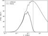Fig. 1. Linear power spectrum (dashed line) computed by CLASS for a standard cosmology and smoothed by a Gaussian window of radius Rf = 4 h−1 Mpc (solid line). The vertical dotted line corresponds to $k_{\mathrm{N}}=\frac{\pi }{2R_{\mathrm{f}}}$ (see Sect. 2.1).

2.1. Problem with filtering

Let us consider the case of a LN field (see Appendix A) that is obtained from a Gaussian field (ν(x)) applying the following local transform to each location:

$$\begin{array}{c}\hfill {\delta }_{\mathrm{LN}}(x)=e^{\nu (x)-\frac{{\sigma }^2}{2}}-1.\end{array}$$(4)

Remarkably, in this case the transformed auto-correlation function is analytical:

$$\begin{array}{c}\hfill {\xi }_{\mathrm{LN}}(r)=e^{{\xi }_{\nu }(r)}-1.\end{array}$$(5)

This suggests a straightforward way for generating an LN field with some target power-spectrum: just log-transform (i.e. apply Eq. (4)) a Gaussian field with a spectrum 𝒫_ν(k) corresponding to

$$\begin{array}{c}\hfill {\xi }_{\nu }(r)=ln(1+{\xi }_{\mathrm{LN}}(r)),\end{array}$$(6)

that we will call an inverse-log transform. By construction, the LN field should then have the desired spectrum.

As shown in Fig. 2, when we do so and compute the power spectrum 𝒫_ν(k) corresponding to Eq. (6), its high k part becomes negative where the spectrum is cut by the window. This prohibits any standard Gaussian shooting method.

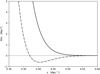Fig. 2. Close-up of Fig. 1. Shown are the smoothed power spectrum (solid line) and the one reconstructed by applying the Eq. (6) inverse-log transform (dash-dotted line).

Indeed any function cannot represent an auto-correlation function since it must be positive definite, which in practical terms is checked by looking at the positivity of its Fourier transform (for an extensive discussion, see Yoglom 1986). This is clearly not the case here where we implicitly assumed that (1+ξ_LN(r)) represents an auto-correlation function. This is very different from the direct log case (Eq. (5)) where the auto-correlation function is constructed from classical statistical rules. This is a small effect, but we cannot be satisfied by clipping all negative values to zero since then the variance of the field would be incorrect and the spectrum biased for high k values.

Let us investigate when the problem happens. Postponing the details to the next section, we compute the 3D power spectrum given by Eq. (6). We count the fraction of modes with negative values with respect to the smoothing size R_f for three N_s samplings (256, 512, and 1024) with a fixed box size corresponding to three values of the grid size a. The outcome of this test is presented in Fig. 3, which shows that in each case modes with negative power appear when R_f ≳ a/2. This means that we can reconstruct a proper LN field as far as R_f >  a/2. This is only partially satisfactory since we may adjust the step size (with N_s) to the smoothing radius, but we will only be able to reconstruct the spectrum up to the Nyquist frequency

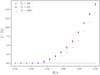Fig. 3. Fraction f− of negative values in the three-dimensional 𝒫ν(k) as a function of the relative filtering Rf/a for three different grid samplings. The ratio Rf/a represents the relative scale between the smoothing scale Rf of the filtered power spectrum and the size of a grid unity a.

$$\begin{array}{c}\hfill k_{\mathrm{N}}={\displaystyle \frac{\pi }{a}}={\displaystyle \frac{\pi }{2R_{\mathrm{f}}}}·\end{array}$$(7)

As illustrated in Fig. 1 (dashed vertical line), we do not sample the spectrum entirely and thus miss a small amount of power. This should affect the variance of the field; however, the power is restituted through aliasing.

There is no fully satisfactory solution to this problem since the procedure itself is mathematically ill defined whenever the spectrum reaches small values. The exact LN sampling of a filtered field cannot be achieved by transforming a Gaussian field.

Fortunately, we do not need to explicitly filter the field. From the density field we generate a discrete set of galaxies, a process that introduces some filtering, but if we exactly control this filtering (as is demonstrated in Sect. 3) we do not need to perform it explicitly at the very start. Then we can work with an unfiltered field (like the dashed one in Fig. 1) that is well-behaved for the transforms. However as Fig. 1 clearly shows, there will always be some extra power above the Nyquist frequency, and thus the key point discussed next is the proper handling of aliasing.

2.2. Taking into account aliasing

Although our method’s grounds are somewhat standard (e.g. Chiang et al. 2013; Greiner & Enßlin 2015; Agrawal et al. 2017; Xavier et al. 2016), we introduce two new aspects:

1. We generalise the PDF to any distribution;

2. We take into account aliasing to deal with the residual power.

The idea to obtain any PDF (for the density contrast δ) is to go into configuration space and apply a non-linear local transform to the Gaussian field ν:

$$\begin{array}{c}\hfill \delta =\mathcal{L}(\nu ).\end{array}$$(8)

The ℒ function can be found easily by applying standard probability transformation rules (Bel et al. 2016) and may need to be computed numerically. In the LN case, the transformation is analytical and is given in Eq. (4).

From now on, δ(x) is assumed to be a real, L periodic, and translational invariant field with null expectation value. Let us define δ_k as its Fourier transform. On the one hand, the translational invariance imposes that the covariance between wave modes is diagonal, ⟨δ_kδ_k′⟩ = δ^D(k + k′)𝒫(k); on the other hand, the periodicity implies that the Fourier transform δ_k is non-zero only for k = nk_f, where k_f = 2π/L is the fundamental frequency of the field and n is an integer vector. Adding the fact that the field is real, it follows that the expectation value of the square modulus of the Fourier transform is directly related to the power spectrum

$$\begin{array}{c}\hfill ⟨|{\delta }_{\mathit{k}}{|}^2⟩=\frac{\mathcal{P}(\mathit{k})}{k_{\mathrm{f}}^3},\end{array}$$(9)

while the covariance between modes remains null. This property allows us to set up a Gaussian field ν_k, following a power spectrum 𝒫_ν(k), in Fourier space by generating two uncorrelated centred Gaussian random variables (the real and the imaginary part of the Fourier density field ν_k). They must have the same variance, which should be equal to half the value of the power spectrum evaluated at the considered k-mode. This is equivalent to generating the square of the modulus of δ_k following an exponential distribution with parameter ${\mathcal{P}}_{\nu }({k})/k_{\text{f}}^3$ and a random phase peaked from a uniform distribution between 0 and 2π. Thus, in practice the Fourier transform of a Gaussian field can be generated on a Fourier grid as

$$\begin{array}{c}\hfill {\nu }_{\mathit{k}}=\sqrt{-{\mathcal{P}}_{\nu }(\mathit{k})/k_{\mathrm{f}}^{3}ln(1-{ϵ}_1)}{e}^{2\pi {ϵ}_2},\end{array}$$(10)

with ϵ₁ and ϵ₂ being two uncorrelated random variables uniformly distributed between 0 and 1. In addition to the appealing property of having a null correlation between different modes, generating a Gaussian field in Fourier space allows us to take avantage of the 3D FFT algorithm. The novel ingredient is to consider that since we are using here a raw (i.e. unfiltered) cosmological spectrum, more power is leaking around the Nyquist frequency.

Then to be coherent with our process of generating the Gaussian field with the required input power spectrum 𝒫_ν(k) we must add the aliased power as an input in Fourier space (see Hockney & Eastwood 1988, for a detailed review), which can be performed by summing the power spectrum aliases

$$\begin{array}{c}\hfill \widehat{\mathcal{P}}(\mathit{k})={\displaystyle \sum _{\mathit{n}}\mathcal{P}\left(|\mathit{k}-2\mathit{n}{k}_{\mathrm{N}}|\right),}\end{array}$$(11)

where n runs over the 3D Fourier wavenumbers. These terms are taken into account at the beginning of the method, as soon as the theoretical power spectrum ${\mathcal{P}}_{\delta }^{\mathrm{th}}(k)$ is provided by CLASS. We note that since the aliasing effect mixes modes that are uncorrelated, the phases remain uniformly distributed in Fourier space while the effective amplitude of the power spectrum changes according to Eq. (11). In our analysis we find that using only the first 125 contributions from n = ( − 2, −2, −2) to n = (2, 2, 2) is enough to reach a percent-level accuracy on the power spectrum of the catalogue at the Nyquist frequency. A more computationally efficient choice would be to take only the first 27 aliases, but it would lead to an accuracy of around 5–6%. In turn, if all alias contributions are discarded, then nearly 2% of the modes would be required to have a negative variance. Clipping these pathological modes to 0 power would lead to a significant deviation of the power spectrum of the generated field with respect to the expected one, even below the Nyquist frequency. In the following we consider the first 125 alias contributions.

As detailed in Bel et al. (2016) any local transform ℒ applied to a centred Gaussian field ν(x) corresponds to a one-to-one mapping λ of its two-point correlation function ξ_ν(r)≡⟨ν(x)ν(x + r)⟩ such that δ(x) = ℒ[ν(x)] and ξ_δ(r) = λ[ξ_ν(r)]. The λ function is given explicitly in Appendix B (Eqs. (B.12) and (B.13)). As a result, using an inverse Fourier transform we can find the 3D two-point correlation of the target non-Gaussian field δ(x), from which, using the inverse mapping λ⁻¹, we are able to compute the corresponding two-point correlation of the Gaussian field ν(x). In the end we only need to perform an inverse Fourier transform in order to get the input power spectrum 𝒫_ν(k) that characterises the input Gaussian field. We can see that being obtained from the Fourier transform of a regularly (grid) sampled two-point correlation, it already contains aliasing effects. Thus, the input Gaussian field can be generated on the corresponding Fourier grid from Eq. (10). A summary of the steps involved in the process computation of the power spectrum 𝒫_ν of the Gaussian field are shown in Fig. 4. Those steps do not require reevaluation for each realisation of the density field. This process can be time consuming so it is better to avoid repeating it when it is not necessary. Both computational time and memory of each array involved in the chain shown in Fig. 4 are summarised in Table 1. We call alias27 and alias125 the number of alias elements added to the raw power spectrum in Eq. (11) (respectively 27 and 125 terms). For ease of comparison, we use a single thread on a 2,4 GHz processor (without considering multiprocessing).

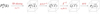Fig. 4. Schematic view of the method used to build the power spectrum involved in the sampling of the Gaussian field, prior to its local transformation. The grey box means that three dimensions are considered.

Finally, we can inverse Fourier transform the realisation of the Gaussian field and apply to it a local transformation, which will automatically turn both the PDF and the power spectrum into the expected ones. It is clear that if the input power spectrum was not aliased (as it naturally is) then the corresponding inverse Fourier transform could not be interpreted as a regularly sampled Gaussian field, thus the process would not be self-consistent.

Figure 5 illustrates the power spectra involved in the generation of the non-Gaussian density field. The raw input power spectrum obtained from the CLASS code and its corresponding aliased version (${\mathcal{P}}_{\delta }^{\text{th}}(\mathit{k})$)) can be seen. We note that the aliasing needs to be applied on the 3D Fourier grid, while we represent only the averaged power spectrum in each Fourier shell of size k_f. In addition, the same Figure shows the corresponding power spectrum of the Gaussian field that we use to generate Monte Carlo realisations. We note an excess of power at large k, which corresponds to the aliasing contribution.

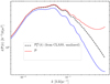Fig. 5. Power spectra involved in the Monte Carlo process. Shown is the theoretical 1D matter power spectrum computed by CLASS (dashed black line). Also shown (in red and blue, respectively) are the shell-averaged power spectra (in shells of width |k|−kf/2 <  |k|< |k|+kf/2) showing the aliased version of the input power spectrum computed by the Boltzmann code and the corresponding power spectrum after transformation (B.12) (see Fig. 4 for details). All of them are plotted up to Nyquist frequency kN ∼ 0.67 h Mpc−1 with a setting of Ns = 256 and L = 1200 h−1 Mpc.

In order to verify the coherency of the method, we generated 1000 realisations of LN non-Gaussian fields in a periodic box of size L = 1200 h⁻¹ Mpc with two different spatial resolutions corresponding to a number of sampling per side of N_s = 256 and 512.

From the definition of the power spectrum (Eq. (9)), we estimated the power spectrum on the 3D Fourier grid by computing the ensemble average of the 1000 realisations and compared it to the true expected power spectrum (${\mathcal{P}}_{\delta }^{\text{th}}(\mathit{k})$). In Fig. 6, we represent the k-shell-averaged relative difference between the estimated and expected power spectrum for each individual wave modes. We can safely conclude that the accuracy of the proposed method is better than 0.1% for wave modes close to the Nyquist frequency. In addition, no significant bias can be detected at the sub-percent level on the whole range of wave modes present in the density field independently from the choice of the spatial resolution.

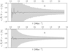Fig. 6. Averaged 3D power spectrum compared to the expected 3D power spectrum, for 1000 realisations of the density field. The shell-averaged monopoles of this residuals in shells of width |k|−kf/2 <  |k|< |k|+kf/2 were then computed. The result is presented as percentage with error bars. The setting used is a sampling number per side of 256 in the top panel and 512 for the other, all in a box of size L = 1200 h−1 Mpc at redshift z = 0. Both results are computed up to the Nyquist frequency.

2.3. Covariance matrix

A possible interest of being able to generate non-Gaussian fields with a Monte Carlo method is related to generating a large number of realisations in order to estimate the covariance matrix (and its inverse) of a cosmological observable with a high level of statistical precision. In the following we define the shell-averaged power spectrum as our observable, and we estimate its covariance matrix between two shells centred around wave numbers k_i and k_j as

$$\begin{array}{c}\hfill \widehat{C}=\frac{{\mathrm{\Delta }}^T\mathrm{\Delta }}{N-1}·\end{array}$$(12)

Here Δ is a matrix formed by the residual between the estimated power spectrum in each realisation and the estimated ensemble average of the power spectrum in each k-shell, and ${\mathrm{\Delta }}_{\mathit{ij}}={\mathcal{P}}_j(k_i)-\overline{\mathcal{P}}(k_i)$ and $\overline{\mathcal{P}}(k_i)=\frac{1}{N}\sum _{j=1}^N{\mathcal{P}}_j(k_i)$, where the j index refers to the j-th realisation. If the deviation elements Δ_ij follow a Gaussian distribution then we can show that the estimated covariance matrix elements C_ij follow a Wishart distribution. As a result, the estimator (12) is unbiased and the variance of the covariance matrix elements (see Anderson 1984) is given by

$$\begin{array}{c}\hfill \mathbb{V}\left[C_{\mathit{ij}}\right]=(C_{\mathit{ij}}^2+C_{\mathit{ii}}{C}_{\mathit{jj}})/(N-1).\end{array}$$(13)

In the following we show that the statistical behaviour of the variance of the estimator of the power spectrum is in agreement with what we expected to find.

Having control of both the target PDF and the power spectrum, we can predict to some extent the expected covariance matrix C of our power spectrum estimator. Since the density field generated with a Monte Carlo process is non-Gaussian, the covariance matrix of the estimator of the power spectrum involves contribution of the Fourier space four-point correlation function. For a translational invariant density field it reduces to

$$\begin{array}{c}\hfill {⟨{\delta }_{{\mathit{k}}_1}{\delta }_{{\mathit{k}}_2}{\delta }_{{\mathit{k}}_3}{\delta }_{{\mathit{k}}_4}⟩}_c={\delta }^D({\mathit{k}}_1+{\mathit{k}}_2+{\mathit{k}}_3+{\mathit{k}}_4)T({\mathit{k}}_1,{\mathit{k}}_2,{\mathit{k}}_3,{\mathit{k}}_4),\end{array}$$(14)

where T is defined as the tri-spectrum which is the Fourier transform of the four-point correlation function in configuration space. As shown by Scoccimarro et al. (1999), the covariance matrix elements of the power spectrum estimator can be expressed as

$$\begin{array}{c}\hfill C_{\mathit{ij}}=\frac{\mathcal{P}{(k_i)}^2}{M_{k_i}}{\delta }_{\mathit{ij}}^D+k_{\mathrm{f}}^3\overline{T}(k_i,k_j),\end{array}$$(15)

where M_ki is the number of independent modes in shell i and

$$\begin{array}{c}\hfill \overline{T}(k_i,k_j)={\displaystyle {\int }_{k_i}{\int }_{k_j}T({\mathit{k}}_1,-{\mathit{k}}_1,{\mathit{k}}_2,-{\mathit{k}}_2)\frac{{\mathrm{d}}^3{\mathit{k}}_1}{V_{k_i}}\frac{{\mathrm{d}}^3{\mathit{k}}_2}{V_{k_j}},}\end{array}$$(16)

where the integral is made over two shells of thickness k_f centred and encapsulating k_i and k_j. The volume (in Fourier space) of each shell containing independent modes is denoted as V_ki and V_kj; in the limit of thin shells we have that V_k = 2πk²k_f thus $M_k=2\pi k^2/k_{\text{f}}^2$.

In Appendix C we show how to predict in a perturbative way the tri-spectrum of the generated non-Gaussian density field for any local transform. In particular, for the contribution of the tri-spectrum to the diagonal elements of the covariance matrix we obtain the expression

$$\begin{array}{cc}& \overline{T}(k_i,k_i)\sim 8c_1^2\{4c_2^2+3c_3{c}_1\}{\mathcal{P}}^3(k_i)\hfill \\ \hfill & +24\{3c_1^2{c}_3^2+4c_1{c}_2^2{c}_3+12c_1^2{c}_2{c}_4\}{\mathcal{P}}^2(k_i){\mathcal{P}}^{(2)}(k_i)\hfill \\ \hfill & +144c_1^2{c}_3^2{\mathcal{P}}^{(2)}(0){\mathcal{P}}^2(k_i),\hfill \end{array}$$(17)

where 𝒫⁽²⁾(k_i ≡ ℱ[ξ²] = ∫𝒫(q)𝒫(|q + k_i|)d³q and the c_n are the coefficients of the Hermite transform of the function ℒ:

$$\begin{array}{c}\hfill c_n=\frac{1}{n!}{\displaystyle {\int }_{-\infty }^{\infty }\mathcal{L}(\nu )H_n(\nu )\frac{e^{\frac{-{\nu }^2}{2}}}{\sqrt{2\pi }}d\nu .}\end{array}$$(18)

Here H_n denotes the probabilistic Hermite polynomial of order n. From Eq. (17) we can see that the covariance matrix elements are expected to depend on both the chosen target power spectrum and the probability density distribution of density fluctuations.

We generate 7375 realisations of a LN density field characterised by a ΛCDM power spectrum at redshift z = 0, the c_n are thus given analytically. We can evaluate the covariance matrix elements of the power spectrum estimator as a simple matrix product (see Eq. (12)). In Fig. 7 we show the diagonal elements, namely the variance at each wave mode compared to the Gaussian contribution and the expected non-Gaussian contribution coming from Eq. (17). It shows a better correspondance between perturbation theory and simulations up to k ∼ 10⁻¹ confirming that for intermediate-wave modes the non-Gaussian correction starts being relevant; however, as expected, it fails to reproduce the full k-dependance because expression (17) was obtained in a perturbative way. In Fig. 8 we show some combinations of modes k_i and k_j of the covariance matrix elements; they exhibit a clear dependance in such combination showing that due to the non-Gaussian nature of the created density field long- and short-wave modes are correlated in our power spectrum estimator.

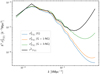Fig. 7. Measured diagonal of the covariance matrix for 7375 power spectra realisations of the density field using the Monte Carlo method (black line) up to kN ∼ 0.67 h Mpc−1. The other curves represent their predictions taking into account the Gaussian part alone (G) or by adding some non-Gaussian contributions of Eq. (15). For example in (1-NG) only the term in 𝒫3(ki) is kept in the tri-spectrum development presented in Eq. (17), while in (3-NG) all of them are kept.

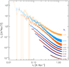Fig. 8. Off-diagonal elements of the covariance matrix estimated with N = 7375 realisations, showing the dependance of the Cij with respect to kj at various fixed ki (see labels on the right). The error bars are computed from Eq. (13).

In the following we extend the case of the continuous sampled density field to the creation of a catalogue of discrete objects, which could be galaxies, clusters, haloes, or simply dark matter particles.

3. Production of a catalogue

3.1. Poisson sampling

Simulating a galaxy catalogue implies transforming the sampled continuous density field δ(x) into a point-like distribution. The density field must therefore be translated into a number of objects (galaxies, haloes, or dark matter particles) per cell imposing an average number density ρ₀ in the comoving volume such that ρ(x) = ρ₀[1 + δ(x)] and performing a Poisson sampling (Layzer 1956). To do so, we must choose an interpolation scheme in order to be able to define a continuous density field ρ⁽ⁱ⁾(x) between the sampling nodes x_j surrounding a cell centred on position x_i. In this way, for each cell i we are able to compute the expected number of object Λ_i as

$$\begin{array}{c}\hfill {\mathrm{\Lambda }}_i={\displaystyle {\int }_{v_i}{\rho }^{(i)}(\mathit{x}){\mathrm{d}}^3\mathit{x},}\end{array}$$(19)

where in practice the integration domain v_i corresponds to the volume of a cell.

Finally, we assign to the cell the corresponding number of galaxies N_i such that the probability of observing N objects given the value of the underlying field Λ is given by a Poisson distribution $P_{\mathrm{N}}=\frac{{\mathrm{\Lambda }}^N}{N!}{e}^{-\mathrm{\Lambda }}$. This means that we can distribute the right number N_i of objects in each cell volume with a spacial probability distribution function proportional to the interpolated density field ρ⁽ⁱ⁾(x) within the cell.

The most straightforward interpolation scheme consists in populating cells uniformly with the corresponding number of objects, which is called the Top-Hat scheme. We can guess that on scales comparable to the size of the randomly populated cells the power spectrum of the Poisson sample will not match the expected power spectrum.

When $\stackrel{\sim }{\delta }(\mathit{x})$ is the sampled density contrast field (the true density contrast field multiplied by a Dirac comb), the corresponding interpolated density contrast within the cell $\widehat{\delta }(\mathit{x})$ is obtained by convolving the sampled density field with a window function W(x) leading in Fourier space to the power spectrum relevant for the Poisson process as $\widehat{\mathcal{P}}(\mathit{k})=\stackrel{\sim }{\mathcal{P}}(\mathit{k}){|W(\mathit{k})|}^2$, where $\stackrel{\sim }{\mathcal{P}}(\mathit{k})$ is the power spectrum of the sampled density field, namely the aliased power spectrum. We can thus finally obtain that the expected power spectrum of the created catalogue is

$$\begin{array}{c}\hfill \widehat{\mathcal{P}}(\mathit{k})={|W(\mathit{k})|}^2{\displaystyle \sum _{\mathit{n}}\mathcal{P}\left(|\mathit{k}-2\mathit{n}{k}_{\mathrm{N}}|\right)+\frac{1/{(2\pi )}^3}{{\rho }_0},}\end{array}$$(20)

where the additional term on the right corresponds to the shot noise contribution due to the auto-correlation of particles with themselves. As anticipated in the previous section, we note that the Fourier transform of the chosen convolution function W is cutting the power on a small scale, which is equivalent to smoothing the density field on the size of the cells.

The interpolation scheme for the number density within each cell defines the form of the smoothing kernel W; in the following we consider two different interpolation schemes. The first (the first order) is the Top-Hat scheme which consists in defining cells around each node of the grid and assigning the corresponding density within the cell. The second (the second order) is a natural extension, which consists in defining a cell as the volume within eight grid nodes and adopting a tri-linear interpolation scheme between the nodes. In any of the two cases the window function (see Sefusatti et al. 2016, for higher order smoothing functions) takes the general form W⁽ⁿ⁾(k) = [j₀(k_xa/2)j₀(k_ya/2)j₀(k_za/2)]ⁿ, where j₀ is the spherical Bessel function of order 0 and the index n corresponds to the order of the interpolation scheme.

We estimate the power spectrum of the catalogues with the method described by Sefusatti et al. (2016) employing a particle assignment scheme of order four (piecewise cubic spline) and the interlacing technique to reduce aliasing effects. We note that these choices are intrinsic to the way we estimate the power spectrum of the distribution of generated objects and has nothing to do with the way we generate the catalogues. In Fig. 9, we compare the power spectra of the catalogues of objects for the two interpolation schemes described above. As expected, on small scales the linear interpolation scheme reduces the extra power more efficiently, due to aliasing.

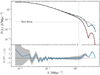Fig. 9. Top: measured power spectra averaged over 100 realisations of the Poissonian LN field for the Top-Hat interpolation scheme (blue curve with prediction in dash-dotted black line) and for the linear interpolation scheme (red curve and prediction in dashed line). The shot noise is subtracted from measures (solid horizontal black line) and is about 3.48 × 10−2 h3 Mpc3. The dotted black curve represents the alias-free theoretical power spectrum computed by CLASS. Bottom: relative deviation in percentage between the averaged realisations (with shot noise contribution) and prediction (with the same shot noise added) in blue line with error bar in grey for the Top-Hat interpolation scheme. Snapshots are computed for a grid of size L = 1200 h−1 Mpc and parameter Ns = 512. Here comparisons are made well beyond the Nyquist (vertical line) frequency at kN ∼ 1.34 h Mpc−1.

In the same figure we also show the expected power spectra computed with Eq. (20) and corresponding to the two mentioned interpolation schemes. We demonstrate in both cases that we control precisely the smoothing of the spectrum up to the Nyquist frequency and even above.

3.2. Light cone

In the following we describe how we build a light cone from our catalogue, and we compare two methods.

Shell method. The first idea is to glue a series of comoving volume at constant time in order to reconstruct the past light cone shell by shell (Fosalba et al. 2015; Crocce et al. 2015). However we take care of keeping track of the cross-correlation between shells by starting with the same Gaussian field for all the shells. In practice, we first select a redshift interval Δz labelled by z_min and z_max and a number N_shl of shells within it. For each of these shells, we generate a point-like distribution in a comoving volume at constant cosmic time. Obviously, we perform the Poisson sampling only of the cells contributing to the considered redshift shell. In addition, we keep only the objects belonging to the comoving volume spanned by the redshift shell, defined by [R(z_i − dz/2),R(z_i + dz/2)], where z_i corresponds to the redshift of the comoving volume, dz = Δz/N_shl, and R(z) is the radial comoving distance. The light cone method is designed to cover 4π steradians on the sky.

In the next section we show the effect of the choice of the number of shells N_shl used to build the light cone, on the angular power spectrum.

Cell method. The second method is faster. Rather than simulating many redshift shells, we select a single redshift z₀ chosen at the middle of the radial comoving space spanned by the light cone. We generate the corresponding Gaussian field in a comoving volume on a grid at z = z₀. At this level we needs to include some evolution in the radial direction from the point of view of an observer located at the centre of the box. To do so, there are two possibilities.

– We can simply think of rescaling the Gaussian field at a comoving radial distance x(z) (from the observer) with the corresponding growth factor D(z), which rules the evolution of linear matter perturbations (Peebles 1980). In this way it is clear that on large scales the power spectrum of the density field will follow the expected evolution in D²(z); however, the small scales will be affected in a non-trivial way leading to a modification of the shape of the power spectrum.

– We can change the contrast field so that the evolution of the density field will follow the growth factor D(z). For the LN case this would read

$$\begin{array}{c}\hfill {\delta }_{\mathrm{LN}}(x,z)=e^{\nu (x,z)-D^2(z)\frac{{\sigma }^2(0)}{2}}-1.\end{array}$$(21)

The second option is particularly well suited when generating a density field following a linear evolution. However the first option, although not exact, can allow for the fast computation of spectra evolution for more complex cases as when D(k, z) depends on k. In the following section we compare, in the linear regime, the shell method and the two cell methods in the case of the LN density field.

We conclude this section by providing the running time for the generation of a catalogue of ∼110 million galaxies with the second method considering that the chain in Fig. 4 has already been computed. We get 1.7 min for N_s = 256, 11 min for N_s = 512 and 1.7 h for N_s = 1024 using a single thread on a 2,4 GHz processor.

4. Application to tomography

In cosmology, several arguments can be put forward to justify a tomographic approach. Unlike the estimation of the power spectrum or the two-point correlation function, no fiducial cosmology needs to be assumed in order to estimate the observable (see Bonvin & Durrer 2011; Montanari & Durrer 2012; Asorey et al. 2012). Only angular observed positions and measured redshift are required, thus making it a true observable quantity. In addition, the observable is defined on a sphere simplifying its combinations with other cosmological probes such as lensing (Cai & Bernstein 2012; Gaztañaga et al. 2012) or CMB and Hα intensity mapping.

4.1. Angular power spectrum C_ℓ

So far we have worked on a Fourier basis, but it is useful to expand the matter perturbations into spherical harmonics (Peebles 1980) and consider its coefficients:

$$\begin{array}{c}\hfill {\delta }_{\ell }^m(r)={\displaystyle {\int }_S\delta (r,\theta ,\varphi ){Y_{\ell }^m}^{\ast }(\theta ,\varphi )d^2\mathrm{\Omega }.}\end{array}$$(22)

Assuming that the field is statistically invariant by rotation, i.e. its angular two-point correlation function only depends on the angular separation and not on the absolute angular position (the analogue of translational invariance in 3D) on the sky, the two-point correlation of the harmonic coefficient depends only on the order ℓ, thus $C_{\mathcal{l}}(r,r^{\prime })\equiv \langle {\delta }_{\mathcal{l}}^m(r){\delta }_{\mathcal{l}}^m{}^{\star }(r^{\prime })\rangle$ is defined as the angular power spectrum between shells r and r′. We may relate this spectrum to the isotropic 3D spectrum as

$$\begin{array}{c}\hfill C_{\ell }(r,r^{\prime })={(4\pi )}^2{\displaystyle {\int }_0^{\infty }{k}^2\mathcal{P}(k)j_{\ell }(kr)j_{\ell }(k{r}^{\prime })\mathrm{d}k,}\end{array}$$(23)

where j_ℓ is the spherical Bessel function of order ℓ. However, in this expression there is an explicit dependence on the radial comoving distances r and r′.

We can project the density field of a thick redshift shell with a given weighting function W(z) and define our observable density field as

$$\begin{array}{c}\hfill {\stackrel{\sim }{\delta }}_1(\theta ,\varphi )={\displaystyle \int W(z)\delta (r(z),\theta ,\varphi )\mathrm{d}z.}\end{array}$$(24)

The corresponding angular power spectrum³ can be predicted from

$$\begin{array}{cc}\hfill C_{\ell }(z_1,z_2)& ={(4\pi )}^2{\displaystyle \int \mathrm{d}z\mathrm{d}{z}^{\prime }W(z)W(z^{\prime })}\hfill \\ \hfill & \times {\displaystyle {\int }_0^{\infty }{k}^2\mathcal{P}(k)j_{\ell }(kr(z))j_{\ell }(k{r}^{\prime }(z))\mathrm{d}k.}\hfill \end{array}$$(25)

In practice, the numerical evaluation of Eq. (25) is not simple and we use the Angpow software (Neveu & Plaszczynski 2018), which is fully optimised for this task.

This theoretical quantity may then be compared to our simulations by considering the number counts within pixels from samples in the z₁ <  z <  z₂ range (i.e. using for W a Top-Hat window) since in our case the only source of fluctuations is due to the overdensity field. We then simply project the objects of the catalogue on the sky, count them, normalise by the mean value within pixels $\overline{N}$, and compute the spherical power-spectrum ${\widehat{C}}_{\ell }$ with the Healpix (Górski et al. 2005) software using the parameter nside = 2¹¹. The shot-noise contribution is classically $\frac{1}{\overline{N}}$. We note that as in the Fig. (9), we compute the angular power spectrum on scales smaller than the grid pitch. On a spherical basis, the equivalent of the Nyquist mode is obtained using ℓ_N ∼ R[z_mean]k_N, where z_mean is the averaged redshift of the particles composing the catalogue.

In Fig. 10 we compare the estimated angular power spectrum in the [0.2, 0.3] redshift range to the predicted one (Eq. (25)) with the shell method described in Sect. 3 (N_shl = 250) for one thousand generated light cones. In the lower panel of the same figure we display the relative difference between the two showing that the agreement is better than the percent level.

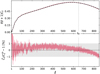Fig. 10. Top panel: one thousand averaged Cℓ values for simulated light cones using the shell method with error bars (red curve) and corresponding prediction (dashed black curve). We simulate here a light cone between redshifts 0.2 and 0.3 in a sampling Ns = 512 and a number of shells Nshl = 250 to ensure a sufficient level of continuity in the density field. The spherical Nyquist mode is situated around ℓN ∼ 650 and represented by the vertical reference. Bottom panel: relative deviation in percent of the averaged predicted Cℓ values with error bars in red.

In order to quantify the impact of the choice of the number of shells in the shell method, we run a test comparison between the cell method and various number of shells N_shl in the cell method. We note that since we are using a power spectrum that is evolving linearly across cosmic time, we know that the shell method is expected to converge to cell method if we rescale the density field with the linear growing mode D(z), as described in Sect. 3. Figure 11 shows the outcome of this analysis, which shows that in the considered redshift range the shell method is indeed converging to the cell method below the percent level as long as the number of shells is greater than 200.

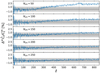Fig. 11. Relative difference in percent between shell method and cell method for varying numbers of shells. The spherical Nyquist mode is situated around ℓN ∼ 650 and represented by the vertical reference.

Finally, we make a comparison within the cell method, rescaling the Gaussian field instead of rescaling the density field. This way we can quantify the deviation when assuming that the Gaussian field evolves linearly when instead it is the density field that is evolving linearly. In Fig. 12, we show the relative deviation in the two cases with respect to the expected power spectrum. We can see that the deviation, despite being systematic, remains small (around the percent level). Therefore, considering these two cell methods, and as stated in the previous section, only the one offering better results will be recommended: the rescaling of the density field (top panel).

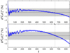Fig. 12. Relative deviation in percent with error bars for 10 000 averaged realisations of Cℓ values in the context of the cell method. In the top panel, the density field (non-Gaussian) is rescaled using linear growth function, while in the bottom panel the Gaussian field following the virtual power spectrum is rescaled. The spherical Nyquist mode is situated around ℓN ∼ 650 and is represented by the vertical reference.

4.2. Covariance matrix

In this section we consider the cell method with linear rescaling of the density field. Our aim is to estimate the covariance matrix of the ${\widehat{C}}_{\ell }$ estimator defined as

$$\begin{array}{c}\hfill {\widehat{C}}_{\ell }\equiv \frac{1}{2\ell +1}{\displaystyle \sum _{m=-\ell }^{\ell }{\stackrel{\sim }{\delta }}_{1,\ell }^m{\stackrel{\sim }{\delta }}_{1,\ell }^{m\star },}\end{array}$$(26)

with a high level of precision. Let us first show that the covariance matrix has a structure similar to the power spectrum estimator studied in Sect. 2. By definition the covariance of ${\widehat{C}}_{\ell }$ is

$$\begin{array}{c}\hfill C_{\ell {\ell }^{\prime }}\equiv \langle {\widehat{C}}_{\ell }{\widehat{C}}_{{\ell }^{\prime }}\rangle -\langle {\widehat{C}}_{\ell }\rangle \langle {\widehat{C}}_{{\ell }^{\prime }}\rangle ,\end{array}$$(27)

where we can substitue ${\widehat{C}}_{\ell }$ with its expression (see Eq. (26)). We immediately see that the first term of Eq. (27) will let a four-point moment appear, which can be expanded (Fry 1984a,b) in terms of cumulative moments (or connected expectation values). It follows that it takes the general form

$$\begin{array}{c}\hfill C_{\ell {\ell }^{\prime }}=\frac{2C_{\ell }^2}{(2\ell +1)}{\delta }_{\ell {\ell }^{\prime }}^K+{\overline{T}}_{\ell {\ell }^{\prime }},\end{array}$$(28)

where ${\overline{T}}_{\ell \ell \prime }$ accounts for non-Gaussian contribution. Instead, when ${\stackrel{\sim }{\delta }}_{\ell }^m$ is a Gaussian field we can see that the covariance matrix is diagonal.

We generate N = 10 000 realisations and measure the angular power spectrum in each of them in order to finally estimate the covariance matrix in the same way as described in Sect. 2. In Fig. 13 we represent the diagonal of the covariance matrix; the errors on the covariance matrix elements are computed with Eq. (13). Since in the Gaussian case the relative error expected on the diagonal of the covariance matrix elements is given by $\sqrt{2/(N-1)}$, the interest of using such a large number of realisations is that we expect a 1.4% precision on the estimation of the diagonal of the covariance matrix and an absolute precision on the correlation coefficients $r_{\mathit{ij}}=C_{\mathit{ij}}/\sqrt{C_{\mathit{ii}}{C}_{\mathit{jj}}}$ of roughly 0.02. In the bottom panel of Fig. 13 we show the relative deviation between the Gaussian prediction and the measured variance of the angular power spectrum, we see that the maximum of deviation is about 45% at ℓ ∼ 600. It appears that deviations from Gaussianity remain small compared to the deviation obtained for the power spectrum covariance matrix, which was about two orders of magnitude bigger (see Sect. 2).

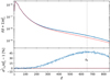Fig. 13. Top: measured diagonal of the covariance matrix (blue curve) over N = 10 000 realisations of different light cones. The red curve represents the associated prediction in the case of a Gaussian field with errors computed using Eq. (13). Here we keep the shot noise (SN) effect in the measures and include it in the prediction. The spherical Nyquist mode is situated around ℓN ∼ 650. Bottom: relative difference in percent following the same colour-coding.

In addition, in Fig. 14 we display some off-diagonal covariance elements with their error bars. Despite some fluctuations it is consistant with zero, indicating that the covariance matrix is close to diagonal, as expected in the Gaussian case (at least for the 300 first elements of the matrix by counting them following the description in the caption). In order to make sure that this is indeed the case, in Fig. 15 we show the correlation coefficients $r_{\mathit{ij}}=C_{\mathit{ij}}/\sqrt{C_{\mathit{ii}}{C}_{\mathit{jj}}}$; we see that the matrix is close to diagonal only considering ℓ <  200. It therefore confirms that projecting a thick redshift shell onto the sky tends to turn the density field more Gaussian. This is compatible with what we would naively expect from the central limit theorem since the projection is made by summing over many values of a non-Gaussian field with some weights. It appears that the resulting distribution should tend to a Gaussian as the volume of the projection increases. However, for large ℓ-values we measure a significant amount of correlation typically of order 10% reaching 30% at ℓ ∼ 600.

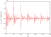Fig. 14. First 300 elements measured for the off-diagonal part of the covariance matrix over n = 10 000 realisations of light cone with Gaussian errors computed using Eq. (13). The elements are labelled by the index m and are ordered column by column in the lower half of the matrix without passing by the diagonal, i.e. Cij,  i >  j.

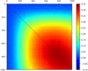Fig. 15. Correlation matrix for 10 000 realisations of Cℓ in a simulated universe between redshifts 0.2 and 0.3 and a sampling Ns = 512. The (ℓ×ℓ′) = (1000 × 1000) of the matrix are represented here.

5. Conclusion

In this paper we refined a known process allowing us to generate a non-Gaussian density field with a given PDF and power spectrum.

We first pointed out the current main mathematical issue arising when we want to generate a density field with a cut-off scale by filtering its power spectrum. We demonstrated that the power spectrum of the Gaussian field that will eventually be transformed into a non-Gaussian is likely to be undefined (i.e. with negative values) on some bandwidth. Even though we noted that there is, in principle, no way of mathematically sorting this problem, we showed that a simple criterion allows a work-around: for a Gaussian filtering, a spatial sampling rate a, which is larger than twice the cut-off scale R_f, needs to be used.

We demonstrated that taking into account aliasing at the stage of generating the density field in Fourier space is of paramount importance in order to maintain the output power spectrum under control. In addition, we showed that without imposing an explicit cut-off scale, at the stage of producing a catalogue with a local Poisson process we introduce an effective filtering of the density field which can be predicted with a sub-percent level accuracy. Regarding the Poisson sampling, we proposed a natural extension of the usual Top-Hat method consisting in populating the cubical cells uniformly with objects: we can linearly interpolate the density field between nodes and populate the cells with a probability distribution following the interpolated density field. The interest of this extension is that it allows us to get closer to the ideal power spectrum by strongly decreasing the amplitude of aliasing.

Regarding the density field, we showed that we can predict in a perturbative way the expected bi-spectrum and tri-spectrum, and we provided an analytical approximation allowing us to predict the variance of the power spectrum estimated for the non-Gaussian density field. This allowed us to check that the statistical behaviour of our method was going in the expected direction.

At the end of Sect. 3 we discussed two different methods to build a light cone out of our catalogues. The shell method can be used whether the evolution of the power spectrum is linear or not, but it involves a large number of redshift shells, which is time consuming. The other method is much faster; the cell method is particularly suitable when the power spectrum evolves linearly, but does not allow us to keep a perfect control on the power spectrum when it presents a non-linear evolution.

Finally, we presented a possible application of this kind of Monte Carlo catalogue of objects to tomographic analysis. We showed that the estimated angular power spectrum is in agreement at the percent level with the expected one. This validated the shell and cell methods used to build the light cones. Thanks to the numerical efficiency of this Monte Carlo we were able to generate 10 000 realisations, allowing us to estimate the covariance matrix elements with a percent accuracy. Despite the reduction of non-Gaussianity involved in the projection of the catalogue on the sky, we were still able to detect a clear signature on small scales, coming from the fact that the catalogues were generated out of a non-Gaussian density field.

Such a Monte Carlo method might be useful in investigating the dependance of the covariance matrix on the cosmological parameter. As recently done by Lippich et al. (2019) and Blot (2019), in a future work we plan to compare the covariance matrix obtained with this method to the one estimated from cosmological N-body simulations and we will include the treatment of redshift space distortions.

References

Appendix A: Some properties of the LN field

Let X follow a Gaussian distribution X ∼ 𝒩(μ,σ²); then Y = e^X follows a LN distribution. For simplicity we consider in the following that the Gaussian has a null mean μ = 0. Its moments can be immediately computed:

$$\begin{array}{cc}\hfill \mathbb{E}\left[y^k\right]& ={\displaystyle {\int }_0^{\infty }{y}^k{f}_Y}(y)\mathrm{d}y={\int }_0^{\infty }{e}^{klny}{f}_Y(y)\mathrm{d}y\hfill \\ \hfill & ={\displaystyle {\int }_{-\infty }^{+\infty }{e}^{\mathit{kx}}\mathcal{N}(x;0,{\sigma }^2)\mathrm{d}x}\hfill \\ \hfill & =e^{k^2{\sigma }^2/2}.\hfill \end{array}$$(A.1)

In particular,

$$\begin{array}{cc}\hfill \mathbb{E}\left[y\right]& =e^{{\sigma }^2/2}\hfill \end{array}$$(A.2)

$$\begin{array}{cc}\hfill \mathbb{V}\left[y\right]& =e^{{\sigma }^2}(e^{{\sigma }^2}-1).\hfill \end{array}$$(A.3)

The idea for cosmology is to ensure a positive energy density (denoted ρ in the following) by transforming a Gaussian density contrast ν into

$$\begin{array}{c}\hfill {\rho }_{\mathrm{LN}}(x)=e^{\nu (x)}.\end{array}$$(A.4)

We recover the LN contrast using Eq. (A.2)

$$\begin{array}{c}\hfill {\delta }_{\mathrm{LN}}={\displaystyle \frac{{\rho }_{\mathrm{LN}}}{\mathbb{E}\left[{\rho }_{\mathrm{LN}}\right]}}-1=e^{\nu -\frac{{\sigma }^2}{2}}-1.\end{array}$$(A.5)

This is a linear transformation of the pure LN distribution e^ν, so we can compute immediately its first two moments:

$$\begin{array}{cc}\hfill \mathbb{E}\left[{\delta }_{\mathrm{LN}}\right]& =0\hfill \end{array}$$(A.6)

$$\begin{array}{cc}\hfill \mathbb{V}\left[{\delta }_{\mathrm{LN}}\right]& ={[e^{-{\sigma }^2/2}]}^2\mathbb{V}\left[{\rho }_{\mathrm{LN}}\right]=e^{{\sigma }^2}-1\hfill \end{array}$$(A.7)

The random field is created by considering it a function of spatial coordinates x_i, and from now on we use the shorthand δ_i = δ(x_i), ν_i = ν(x_i) and ρ_i = ρ(x_i), dropping the “LN” subscript. Its auto-correlation function, assuming isotropy, reads

$$\begin{array}{c}\hfill \xi (r)=\mathbb{E}\left[{\delta }_1{\delta }_2\right]={\displaystyle \frac{\mathbb{E}\left[({\rho }_1-\overline{\rho })({\rho }_2-\overline{\rho })\right]}{\mathbb{E}\left[{\rho }^2\right]}}={\displaystyle \frac{\mathbb{E}\left[{\rho }_1{\rho }_2\right]}{\mathbb{E}{\left[\rho \right]}^2}}-1\end{array}$$(A.8)

Calling f₂(ρ₁, ρ₂) the 2D density distribution of the LN energy density random field, probability conservation yields

$$\begin{array}{c}\hfill f_2({\rho }_1,{\rho }_2)d{\rho }_{1}d{\rho }_2=\mathcal{N}({\nu }_1,{\nu }_2;\mathbf{C})d{\nu }_{1}d{\nu }_2\end{array}$$(A.9)

The covariance matrix of the Gaussian field being

$$\begin{array}{c}\hfill \mathbf{C}=\mathbb{E}\left[{\nu }_1{\nu }_2\right]=\left(\begin{array}{cc}{\sigma }^2& {\xi }_{\nu }\\ {\xi }_{\nu }& {\sigma }^2\end{array}\right),\end{array}$$(A.10)

we can then compute its two-point function in a way similar to moments

$$\begin{array}{cc}\hfill \mathbb{E}\left[{\rho }_1{\rho }_2\right]& ={\displaystyle \int \int e^{ln{\rho }_1}{e}^{ln{\rho }_2}{f}_2({\rho }_1,{\rho }_2)d{\rho }_{1}d{\rho }_2}\hfill \end{array}$$(A.11)

$$\begin{array}{cc}& ={\displaystyle \int \int e^{{\nu }_1}{e}^{{\nu }_2}\mathcal{N}({\nu }_1,{\nu }_2;\mathbf{C})d{\nu }_{1}d{\nu }_2}\hfill \end{array}$$(A.12)

$$\begin{array}{cc}& =e^{{\sigma }^2+\xi }.\hfill \end{array}$$(A.13)

The last line can be obtained from a direct computation or by recalling that the generative functional of a multi-dimensional Gaussian is

$$\begin{array}{c}\hfill \mathbb{E}\left[e^{\mathit{xt}}\right]=e^{\frac{1}{2}{t}^T\mathbf{C}t},\end{array}$$(A.14)

where x, t represent vectors.

Finally, using Eqs. (A.4) and (A.2), we obtain for the contrast density of the LN field the result that

$$\begin{array}{c}\hfill {\xi }_{\mathrm{LN}}(r)=e^{{\xi }_{\nu }(r)}-1\end{array}$$(A.15)

We can check that the variance (ξ(r = 0)) indeed follows Eq. (A.7).

Appendix B: The Mehler formalism

The Mehler transform for bivariate distributions is not a well-known tool, while it is particularly convenient to ease computations of 2D integrals involving Gaussian distributions, as was demonstrated in Simpson et al. (2013) or more recently in Bel et al. (2016).

Let (X₁, X₂) follow a central bivariate distribution

$$\begin{array}{c}\hfill (X_1,X_2)\sim {\mathcal{N}}_2(0,\mathbf{\Sigma }),\end{array}$$(B.1)

with a covariance matrix

$$\begin{array}{c}\hfill \mathbf{\Sigma }=\left(\begin{array}{cc}1& {\xi }_X\\ {\xi }_X& 1\end{array}\right).\end{array}$$(B.2)

For convenience we restrict the variance term to 1, so that the covariance term ξ_ν is the correlation coefficient, and we show at the end of this appendix how to treat the general case. By denoting, in loose notation, 𝒩(x) as the 1D normal distribution, the transform reads

$$\begin{array}{c}\hfill {\mathcal{N}}_2(x_1,x_2)=\mathcal{N}(x_1)\mathcal{N}(x_2){\displaystyle \sum _{n=0}^{\infty }{H}_n(x_1)H_n(x_2){\displaystyle \frac{{\xi }_X^n}{n!}},}\end{array}$$(B.3)

where H_n are the (probabilistic) Hermite polynomials which are orthogonal with respect to the Gaussian measure

$$\begin{array}{c}\hfill {\displaystyle {\int }_{-\infty }^{+\infty }{H}_n(x)H_m(x)\mathcal{N}(x)\mathrm{d}x=n!{\delta }_{\mathit{nm}}.}\end{array}$$(B.4)

The interest here is that when applying some local transform to a Gaussian field Y = ℒ(X) the covariance of the transformed field becomes

$$\begin{array}{cc}\hfill {\xi }_Y=\mathbb{E}\left[y_1{y}_2\right]& ={\displaystyle {\int }_{-\infty }^{\infty }{\int }_{-\infty }^{\infty }{y}_1{y}_2{f}_Y(y_1,y_2)\mathrm{d}{y}_1\mathrm{d}{y}_2}\hfill \\ \hfill & ={\displaystyle {\int }_{-\infty }^{\infty }{\int }_{-\infty }^{\infty }\mathcal{L}(x_1)\mathcal{L}(x_2){\mathcal{N}}_2(x_1,x_2)\mathrm{d}{x}_1\mathrm{d}{x}_2.}\hfill \end{array}$$(B.5)

Then if we decompose the local field onto the Hermite polynomials,

$$\begin{array}{c}\hfill \mathcal{L}(x)={\displaystyle \sum _{n=0}^{\infty }{c}_n{H}_n(x),}\end{array}$$(B.6)

and use the orthogonality properties, we obtain the simple expansion

$$\begin{array}{c}\hfill {\xi }_Y={\displaystyle \sum _{n=0}^{\infty }n!c_n^2{\xi }_G^n,}\end{array}$$(B.7)

where

$$\begin{array}{c}\hfill c_n={\displaystyle \frac{1}{n!}}{\displaystyle {\int }_{-\infty }^{+\infty }\mathcal{L}(x)H_n(x)\mathcal{N}(x)\mathrm{d}x.}\end{array}$$(B.8)

An important point to notice is that all the coefficients in the expansion are positive. Compare this to the series expansion of the inverse log-transform (Eq. (6)). We see immediately that a field with a ln(1 + ξ_X) covariance cannot be obtained from a Gaussian one.

Let us now reconsider the classical LN field (but with σ = 1). The local transform reads

$$\begin{array}{c}\hfill \mathcal{L}(x)=e^{x-1/2}-1.\end{array}$$(B.9)

Then

$$\begin{array}{cc}\hfill c_n& ={\displaystyle \frac{1}{n!}}{\displaystyle {\int }_{-\infty }^{+\infty }(e^{x-1/2}-1)\mathcal{N}(x)H_n(x)\mathrm{d}x}\hfill \\ \hfill & ={\displaystyle \frac{1}{n!}}\left[{\displaystyle {\int }_{-\infty }^{+\infty }\mathcal{N}(x-1)H_n(x)\mathrm{d}x-{\int }_{-\infty }^{+\infty }\mathcal{N}(x)H_n(x)\mathrm{d}x}\right]\hfill \\ \hfill & ={\displaystyle \frac{1}{n!}}[1-{\delta }_{n0}],\hfill \end{array}$$(B.10)

where we used the 𝒩(x) expression, H₀(x) = 1 and ${\displaystyle H_n(x+1)=\sum _{k=0}^n\left(\genfrac{}{}{0pt}{}{n}{k}\right)H_{n-k}(x)}$.

From Eq. (B.7) the autocorrelation of the LN field is

$$\begin{array}{c}\hfill {\xi }_Y={\displaystyle \sum _{n=1}^{\infty }{\displaystyle \frac{{\xi }_G}{n!}}=e^{{\xi }_G}-1,}\end{array}$$(B.11)

in agreement with the more classical way to derive it shown in Appendix A. While unnecessary in the LN case, such an approach is very powerful in computing numerically the auto-correlation of any transformed Gaussian field.

When the Gaussian field does not have a unit variance σ² = ξ_X(0)≠1 which is generally the case, we works with rescaled variables leading to

$$\begin{array}{cc}\hfill {\xi }_Y& ={\displaystyle \sum _{n=0}^{\infty }n!c_n^2{\left({\displaystyle \frac{{\xi }_{\nu }}{{\sigma }^2}}\right)}^n,}\hfill \end{array}$$(B.12)

$$\begin{array}{cc}\hfill c_n& ={\displaystyle \frac{1}{n!}}{\displaystyle {\int }_{-\infty }^{+\infty }\mathcal{L}(\sigma x)H_n(x)\mathcal{N}(x)\mathrm{d}x.}\hfill \end{array}$$(B.13)

Then using the more general local transform discussed in Appendix A,

$$\begin{array}{c}\hfill \mathcal{L}(x)=e^{x-{\sigma }^2/2}-1,\end{array}$$(B.14)

we recover Eq. (B.11).

Appendix C: Higher order correlation functions

In this appendix we show how to predict in a perturbative way the bi-spectrum and tri-spectrum, a non-Gaussian density field generated from the local transformation of a Gaussian field.

Let us consider a density field ϵ(x) in configuration space. We can therefore define its Fourier transform as

$$\begin{array}{c}\hfill {ϵ}_{\mathit{k}}=\mathcal{F}[ϵ(\mathit{x})]\equiv \frac{1}{{(2\pi )}^3}{\displaystyle \int ϵ(\mathit{x})e^{-\mathit{k}·\mathit{x}}{\mathrm{d}}^3\mathit{x}.}\end{array}$$(C.1)

As explained is Sect. 2.2 we generate a Gaussian random field in Fourier space (assuming a power spectrum), we perform an inverse Fourier transform to get its analogue in configuration space. We further apply a local transform ℒ to map the Gaussian field into a stochastic field that is characterised by a target PDF. Thus, the N-point moments can in principle be predicted as soon as the local transform and the target power spectrum have been specified.

Let ν be a stochastic field following a centred (⟨ν⟩ = 0) reduced (${\sigma }_{\nu }^2\equiv {\langle {\nu }^2\rangle }_c=1$) Gaussian distribution. From a realisation of this field, we can generate a non-Gaussian density field δ by applying a local mapping ℒ between the two, hence

$$\begin{array}{c}\hfill \delta =\mathcal{L}(\nu ).\end{array}$$(C.2)

Without a lake of generality, we can express the N-point moments of the transformed density field with respect to the two-point correlation of the Gaussian field as

$$\begin{array}{c}\hfill ⟨{\delta }_1...{\delta }_{\mathrm{N}}⟩={\displaystyle \int \mathcal{L}({\nu }_1)...\mathcal{L}({\nu }_{\mathrm{N}}){\mathcal{B}}^{(N)}(\mathit{\nu },C_{\nu })\mathrm{d}{\nu }_1...\mathrm{d}{\nu }_{\mathrm{N}},}\end{array}$$(C.3)

where ℬ^(N) is a N-variate Gaussian distribution with a N × N covariance matrix C_ν and sub-indexes are referring to positions δ₁ ≡ δ(x₁). In practice, the computation of Eq. (C.3) can be numerically expensive; however, as shown in Appendix B it can be efficiently computed thanks to the Mehler expansion, at least in the case of the two-point moment (see Eq. (B.7)). Assuming that in the local transform ℒ the amplitude of the coefficients of its Hermite transform (see Eq. (B.8)) is decreasing by the order n, it offers the possibility of ordering the various contributions to the total moment.

In order to evaluate Eq. (C.3) we can use extensions of the Mehler formula (Carlitz 1970); for example, the third order leads to

$$\begin{array}{c}\hfill {\mathcal{B}}^{(3)}(\mathit{\nu },C_{\nu })={\displaystyle \sum _{m,n,p}^{\infty }\frac{H_{n+p}({\nu }_1)}{m!}\frac{H_{p+m}({\nu }_2)}{n!}\frac{H_{n+m}({\nu }_3)}{p!}{\xi }_{23}^m{\xi }_{13}^n{\xi }_{12}^p{G}^{(3)}(\mathit{\nu }),}\end{array}$$(C.4)

where the correlation functions ξ₁₂, ξ₁₃, and ξ₂₃ are the three off-diagonal elements of the covariance matrix C_ν and the function G^N is defined as an N-variate Gaussian distribution with a diagonal covariance matrix whose values are all set to unity

$$\begin{array}{c}\hfill G^{(N)}(\mathit{\nu })\equiv \frac{1}{{(2\pi )}^{N/2}}{e}^{-\frac{1}{2}({\nu }_1^2+...+{\nu }_{\mathrm{N}}^2)}.\end{array}$$(C.5)

At fourth order (N = 4), the four-variate Gaussian can be expressed as

$$\begin{array}{cc}\hfill {\mathcal{B}}^{(4)}(\mathit{\nu },C_{\nu })& ={\displaystyle \sum _{l,m,n,o,p,q}^{\infty }\frac{H_{l+m+n}({\nu }_1)H_{l+o+p}({\nu }_2)H_{m+o+q}({\nu }_3)H_{n+p+q}({\nu }_4)}{l!m!n!o!p!q!}}\hfill \\ \hfill & {\xi }_{12}^l{\xi }_{13}^m{\xi }_{14}^n{\xi }_{23}^o{\xi }_{24}^p{\xi }_{34}^q{G}^{(4)}(\mathit{\nu }),\hfill \end{array}$$(C.6)

where again ξ₁₂, ξ₁₃, ξ₁₄, ξ₂₃, ξ₂₄, and ξ₃₄ are the six off-diagonal elements of the covariance matrix C_ν. By replacing Eqs. (C.4) and (C.6) in expression C.3, we can integrate over the N variables ν₁ to ν_N and express the three- and four-point moments as a sum over the product of the two-point correlation function of the Gaussian field

$$\begin{array}{c}\hfill ⟨{\delta }_1{\delta }_2{\delta }_3⟩={\displaystyle \sum _{m,n,p}^{\infty }\frac{(n+p)!(p+m)!(n+m)!}{m!n!p!}{c}_{n+p}{c}_{p+m}{c}_{n+m}{\xi }_{23}^m{\xi }_{13}^n{\xi }_{12}^p}\end{array}$$(C.7)

and

$$\begin{array}{cc}\hfill ⟨{\delta }_1{\delta }_2{\delta }_3{\delta }_4⟩& ={\displaystyle {\sum }_{l,m,n,o,p,q}^{\infty }\frac{(l+m+n)!(l+o+p)!(m+o+q)!(n+p+q)!}{l!m!n!o!p!q!}}\hfill \\ \hfill & c_{l+m+n}{c}_{l+o+p}{c}_{m+o+q}{c}_{n+p+q}{\xi }_{12}^l{\xi }_{13}^m{\xi }_{14}^n{\xi }_{23}^o{\xi }_{24}^p{\xi }_{34}^q,\hfill \end{array}$$(C.8)

where the coefficients c_i are still the coefficients of the Hermite expansion defined by Eq. (B.8). Equations (C.7) and (C.8) are particularly useful when we wants to evaluate the three- and four-point correlation functions of the density field δ or their Fourier counterparts, the bi-spectrum and tri-spectrum.

Let us express first the power spectrum of the density field δ with respect to the power spectrum of the Gaussian field ν. By performing a Fourier transform on Eq. (B.7) we can obtain

$$\begin{array}{c}\hfill {\mathcal{P}}_{\delta }(k)=c_1^2\mathcal{P}(k)+{\displaystyle \sum _{n=2}^{\infty }n!c_n^2{\mathcal{P}}^{(n)}(k),}\end{array}$$(C.9)

where 𝒫⁽ⁿ⁾(k) represents what we call loop corrections of order n − 1 and are defined as ${\mathcal{P}}^{(n)}(k)\equiv \mathcal{F}[{\xi }_{\nu }^n]$. The leading order or tree-level contribution is given by $c_1^2\mathcal{P}(k)$, which is just a change in amplitude of the power spectrum of the Gaussian field. It represents the change in the power spectrum that we would expect if the local transformation ℒ were linear.

We now express the three-point correlation function ζ_δ, 123 ≡ ⟨δ₁δ₂δ₃⟩_c, dropping terms higher than one-loop corrections that we would obtain:

$$\begin{array}{cc}\hfill {\zeta }_{\delta ,123}& \simeq 2c_2{c}_1^2[{\xi }_{12}{\xi }_{13}+{\xi }_{12}{\xi }_{23}+{\xi }_{13}{\xi }_{23}]\hfill \\ \hfill & +6c_3{c}_1{c}_2[{\xi }_{12}{\xi }_{13}^2+{\xi }_{12}{\xi }_{23}^2+{\xi }_{13}{\xi }_{23}^2+{\xi }_{12}^2{\xi }_{13}+{\xi }_{12}^2{\xi }_{23}+{\xi }_{13}^2{\xi }_{23}]\hfill \\ \hfill & +8c_2^3{\xi }_{12}{\xi }_{13}{\xi }_{23}.\hfill \end{array}$$(C.10)

Taking the Fourier transform of the above Eq. (C.10) we can obtain the expression of the bi-spectrum of the density field as

$$\begin{array}{cc}\hfill B_{\delta }(k_1,k_2)& \simeq 2c_2{c}_1^2[\mathcal{P}(k_1)\mathcal{P}(k_2)+\mathcal{P}(k_1)\mathcal{P}(k_{12})+\mathcal{P}(k_2)\mathcal{P}(k_{12})]\hfill \\ \hfill & +6c_3{c}_1{c}_2[\mathcal{P}(k_1){\mathcal{P}}^{(2)}(k_2)+\mathcal{P}(k_1){\mathcal{P}}^{(2)}(k_{12})+\mathcal{P}(k_2){\mathcal{P}}^{(2)}(k_{12})\hfill \\ \hfill & +{\mathcal{P}}^{(2)}(k_1)\mathcal{P}(k_2)+{\mathcal{P}}^{(2)}(k_1)\mathcal{P}(k_{12})+{\mathcal{P}}^{(2)}(k_2)\mathcal{P}(k_{12})]\hfill \\ \hfill & +8c_2^3{B}^{(3)}(k_1,k_2),\hfill \end{array}$$(C.11)

where we use the shorthand notations k_i = k_i, k_ij = |k_i + k_j| and

$$\begin{array}{c}\hfill B^{(3)}(k_1,k_2)\equiv \frac{1}{{(2\pi )}^6}{\displaystyle \int \xi (r)\xi (s)\xi (|\mathit{s}-\mathit{r}|)e^{-i{\mathit{k}}_1·\mathit{r}-i{\mathit{k}}_2·\mathit{s}}{\mathrm{d}}^3\mathit{r}{\mathrm{d}}^3\mathit{s},}\end{array}$$(C.12)

which can also be expressed in terms of a triple product of the power spectrum at different wave modes

$$\begin{array}{c}\hfill B^{(3)}(k_1,k_2)={\displaystyle \int \mathcal{P}(q)\mathcal{P}(|\mathit{q}+{\mathit{k}}_1|)\mathcal{P}(|\mathit{q}-{\mathit{k}}_2|){\mathrm{d}}^3\mathit{q}.}\end{array}$$(C.13)

In the very same way, we can also express the one-loop prediction of the tri-spectrum; we need to start from the four-point correlation function η_δ, 1234 ≡ ⟨δ₁δ₂δ₃δ₄⟩_c = ⟨δ₁δ₂δ₃δ₄⟩−ξ_δ, 12ξ_δ, 34 − ξ_δ, 13ξ_δ, 24 − ξ_δ, 14ξ_δ, 23 (Fry 1984b), where we need to express the products of two-point correlation functions at fourth order, and it follows that

$$\begin{array}{cc}\hfill {\xi }_{\delta ,12}{\xi }_{\delta ,34}& \simeq c_1^4{\xi }_{12}{\xi }_{34}+2c_2^2{c}_1^2[{\xi }_{12}^2{\xi }_{34}+{\xi }_{12}{\xi }_{34}^2]+4c_2^4{\xi }_{12}^2{\xi }_{34}^2\hfill \\ \hfill & +6c_3^2{c}_1^2[{\xi }_{12}^3{\xi }_{34}+{\xi }_{12}{\xi }_{34}^3].\hfill \end{array}$$(C.14)

Keeping terms of order lower or equal to four in terms of ξ in Eq. (C.8) and subtracting permutations of Eq. (C.14) we can obtain the one-loop expression of the four-point correlation function

$$\begin{array}{cc}\hfill {\eta }_{\delta ,1234}& \simeq 6c_3{c}_1^3[{\xi }_{12}{\xi }_{13}{\xi }_{14}+3\mathrm{perm}.]+4c_2^2{c}_1^2[{\xi }_{12}{\xi }_{23}{\xi }_{34}+11\mathrm{perm}.]\hfill \\ \hfill & +18c_1^2{c}_3^2[{\xi }_{12}{\xi }_{13}^2{\xi }_{34}+11\mathrm{perm}.]\hfill \\ \hfill & +12c_3{c}_2^2{c}_1[{\xi }_{12}{\xi }_{13}{\xi }_{34}({\xi }_{12}+{\xi }_{34})+11\mathrm{perm}.]\hfill \\ \hfill & +24c_4{c}_2{c}_1^2[{\xi }_{12}{\xi }_{13}{\xi }_{14}({\xi }_{12}+{\xi }_{13}+{\xi }_{14})+3\mathrm{perm}.]\hfill \\ \hfill & +24c_1{c}_2^2{c}_3[{\xi }_{12}{\xi }_{34}({\xi }_{13}{\xi }_{14}+{\xi }_{23}{\xi }_{24}+{\xi }_{13}{\xi }_{23}+{\xi }_{14}{\xi }_{24})+2\mathrm{perm}.]\hfill \\ \hfill & +16c_2^4[{\xi }_{12}{\xi }_{14}{\xi }_{23}{\xi }_{34}+2\mathrm{perm}.].\hfill \end{array}$$(C.15)

In order to recover the correct permutations, it should be noted that ξ₁₂ and ξ₃₄, ξ₁₃ and ξ₂₄, ξ₁₄ and ξ₂₃ can be interchanged without modification of the coefficients in front, thus in the second line we have four permutations involving the product ξ₁₂ξ₃₄ and we can iterate three times by taking the mentioned specific pairs (ξ₁₂ξ₃₄, ξ₁₃ξ₂₄, and ξ₁₄ξ₂₃). The above expression can be transformed into the tri-spectrum by just taking its Fourier transform, which reads

$$\begin{array}{cc}\hfill T_{\delta }(k_1,k_2,k_3)& \simeq 4c_2^2{c}_1^2\{\mathcal{P}(k_1)\mathcal{P}(k_2)[\mathcal{P}(k_{13})+\mathcal{P}(k_{14})]+5\mathrm{perm}.\}\hfill \\ \hfill & +6c_3{c}_1^3\{\mathcal{P}(k_1)\mathcal{P}(k_2)\mathcal{P}(k_3)+3\mathrm{perm}.\}\hfill \\ \hfill & +18c_1^2{c}_3^2\{{\mathcal{P}}^{(2)}(k_{12})\mathcal{P}(k_1)\mathcal{P}(k_3)+11\mathrm{perm}.\}\hfill \\ \hfill & +12c_3{c}_2^2{c}_1\{\mathcal{P}(k_{12})[{\mathcal{P}}^{(2)}(k_1)\mathcal{P}(k_3)+\mathcal{P}(k_1){\mathcal{P}}^{(2)}(k_3)]+11\mathrm{perm}.\}\hfill \\ \hfill & +24c_4{c}_2{c}_1^2\{\mathcal{P}(k_1)\mathcal{P}(k_2){\mathcal{P}}^{(2)}(k_3)+11\mathrm{perm}.\}\hfill \\ \hfill & +24c_3{c}_2^2{c}_1\{\mathcal{P}(k_1)B^{(3)}(k_2,k_3)+11\mathrm{perm}.\}\hfill \\ \hfill & +16c_2^4\{T^{(4)}(k_1,k_2,k_{14})+T^{(4)}(k_1,k_3,k_{12})+T^{(4)}(k_1,k_4,k_{13})\},\hfill \end{array}$$(C.16)

where we define the fourth order tri-spectrum as

$$\begin{array}{c}\hfill T^{(4)}(k_1,k_2,k_3)\equiv {\displaystyle \int \mathcal{P}(q)\mathcal{P}(|\mathit{q}+{\mathit{k}}_1|)\mathcal{P}(|\mathit{q}-{\mathit{k}}_2|)\mathcal{P}(|\mathit{q}+{\mathit{k}}_3|){\mathrm{d}}^3\mathit{q}.}\end{array}$$(C.17)

References

- Adler, R. J. 1981, The Geometry of Random Fields (London: Wiley) [Google Scholar]
- Agrawal, A., Makiya, R., Chiang, C.-T., et al. 2017, JCAP, 2017, 003 [CrossRef] [Google Scholar]
- Anderson, T. W. 1984, An Introduction to Multivariate Statistical Analysis, 2nd edn. (Wiley Series in Probability and Mathematical Statistics) [Google Scholar]
- Asorey, J., Crocce, M., Gaztañaga, E., & Lewis, A. 2012, MNRAS, 427, 1891 [NASA ADS] [CrossRef] [Google Scholar]
- Bel, J., Branchini, E., Di Porto, C., et al. 2016, A&A, 588, A51 [NASA ADS] [CrossRef] [EDP Sciences] [Google Scholar]
- Blas, D., Lesgourgues, J., & Tram, T. 2011, JCAP, 1107, 034 [NASA ADS] [CrossRef] [Google Scholar]
- Blot, L., Crocce, M., Sefusatti, E., et al. 2019, MNRAS, 485, 2806 [NASA ADS] [CrossRef] [Google Scholar]
- Bonvin, C., & Durrer, R. 2011, Phys. Rev. D, 84, 063505 [NASA ADS] [CrossRef] [Google Scholar]
- Cai, Y.-C., & Bernstein, G. 2012, MNRAS, 422, 1045 [NASA ADS] [CrossRef] [Google Scholar]
- Carlitz, L. 1970, Collect. Math., 21, 117 [Google Scholar]
- Chiang, C.-T., Wullstein, P., Jeong, D., et al. 2013, JCAP, 2013, 030 [NASA ADS] [CrossRef] [Google Scholar]
- Clerkin, L., Kirk, D., Manera, M., et al. 2017, MNRAS, 466, 1444 [NASA ADS] [CrossRef] [Google Scholar]
- Codis, S., Pichon, C., Bernardeau, F., Uhlemann, C., & Prunet, S. 2016, MNRAS, 460, 1549 [NASA ADS] [CrossRef] [Google Scholar]
- Coles, P., & Barrow, J. D. 1987, MNRAS, 228, 407 [NASA ADS] [CrossRef] [Google Scholar]
- Coles, P., & Jones, B. 1991, MNRAS, 248, 1 [NASA ADS] [CrossRef] [Google Scholar]
- Coles, P., & Lucchin, F. 2003, Cosmology, the Origin and Evolution of Cosmic Structure (London: Wiley) [Google Scholar]
- Colombi, S. 1994, ApJ, 435, 536 [NASA ADS] [CrossRef] [Google Scholar]
- Crocce, M., Castander, F. J., Gaztañaga, E., Fosalba, P., & Carretero, J. 2015, MNRAS, 453, 1513 [NASA ADS] [CrossRef] [Google Scholar]
- Fosalba, P., Crocce, M., Gaztañaga, E., & Castander, F. J. 2015, MNRAS, 448, 2987 [NASA ADS] [CrossRef] [Google Scholar]
- Fry, J. N. 1984a, ApJ, 277, L5 [NASA ADS] [CrossRef] [Google Scholar]
- Fry, J. N. 1984b, ApJ, 279, 499 [NASA ADS] [CrossRef] [Google Scholar]
- Gaztañaga, E., Fosalba, P., & Elizalde, E. 2000, ApJ, 539, 522 [NASA ADS] [CrossRef] [Google Scholar]
- Gaztañaga, E., Eriksen, M., Crocce, M., et al. 2012, MNRAS, 422, 2904 [NASA ADS] [CrossRef] [Google Scholar]
- Górski, K. M., Hivon, E., Banday, A. J., et al. 2005, ApJ, 622, 759 [NASA ADS] [CrossRef] [Google Scholar]
- Greiner, M., & Enßlin, T. A. 2015, A&A, 574, A86 [NASA ADS] [CrossRef] [EDP Sciences] [Google Scholar]
- Hamilton, A. J. S. 2000, MNRAS, 312, 257 [NASA ADS] [CrossRef] [Google Scholar]
- Hockney, R. W., & Eastwood, J. W. 1988, Computer Simulation Using Particles (Bristol, PA, USA: Taylor & Francis, Inc.) [CrossRef] [Google Scholar]
- Hubble, E. 1934, ApJ, 79, 8 [NASA ADS] [CrossRef] [Google Scholar]
- Klypin, A., Prada, F., Betancort-Rijo, J., & Albareti, F. D. 2018, MNRAS, 481, 4588 [CrossRef] [Google Scholar]
- Layzer, D. 1956, AJ, 61, 383 [NASA ADS] [CrossRef] [Google Scholar]
- Lippich, M., Sánchez, A. G., Colavincenzo, M., et al. 2019, MNRAS, 482, 1786 [NASA ADS] [CrossRef] [Google Scholar]
- Montanari, F., & Durrer, R. 2012, Phys. Rev. D, 86, 063503 [NASA ADS] [CrossRef] [Google Scholar]
- Neveu, J., & Plaszczynski, S. 2018, Astrophysics Source Code Library [record ascl:1807.012] [Google Scholar]
- Peebles, P. J. E. 1980, The Large-scale Structure of the Universe (Princeton: Princeton University Press) [Google Scholar]
- Scoccimarro, R., Zaldarriaga, M., & Hui, L. 1999, ApJ, 527, 1 [NASA ADS] [CrossRef] [Google Scholar]
- Sefusatti, E., Crocce, M., Scoccimarro, R., & Couchman, H. M. P. 2016, MNRAS, 460, 3624 [NASA ADS] [CrossRef] [Google Scholar]
- Simpson, F., Heavens, A. F., & Heymans, C. 2013, Phys. Rev. D, 88, 083510 [NASA ADS] [CrossRef] [Google Scholar]
- Uhlemann, C., Codis, S., Pichon, C., Bernardeau, F., & Reimberg, P. 2016, MNRAS, 460, 1529 [NASA ADS] [CrossRef] [Google Scholar]
- Xavier, H. S., Abdalla, F. B., & Joachimi, B. 2016, MNRAS, 459, 3693 [NASA ADS] [CrossRef] [Google Scholar]
- Yoglom, A. 1986, Correlation Theory of Stationary and Related Random Functions, Volume I: Basic Results (Spinger Series in Statistics) [Google Scholar]