| Issue |
A&A
Volume 692, December 2024
|
|
|---|---|---|
| Article Number | A260 | |
| Number of page(s) | 23 | |
| Section | Numerical methods and codes | |
| DOI | https://doi.org/10.1051/0004-6361/202452361 | |
| Published online | 18 December 2024 | |
PICZL: Image-based photometric redshifts for AGN
1
Max-Planck-Institut für extraterrestrische Physik,
Giessenbachstr. 1,
85748
Garching,
Germany
2
Exzellenzcluster ORIGINS,
Boltzmannstr. 2,
85748
Garching,
Germany
3
LMU Munich, Arnold Sommerfeld Center for Theoretical Physics,
Theresienstr. 37
80333
München,
Germany
4
LMU Munich, Universitäts-Sternwarte,
Scheinerstr. 1,
81679
München,
Germany
5
Technical University of Munich Department of Computer Science -
I26 Boltzmannstr. 3
85748
Garching b. München,
Germany
6
Max Planck Institut für Astronomie,
Königstuhl 17,
69117
Heidelberg,
Germany
7
Instituto de Astrofísica, Facultad de Física, Pontificia Universidad Católica de Chile,
Campus San Joaquín, Av. Vicuña Mackenna 4860,
Macul Santiago
7820436,
Chile
8
Centro de Astroingeniería, Facultad de Física, Pontificia Universidad Católica de Chile, Campus San Joaquín,
Av. Vicuña Mackenna 4860, Macul
Santiago
7820436,
Chile
9
Millennium Institute of Astrophysics,
Nuncio Monseñor Sótero Sanz 100, Of 104, Providencia,
Santiago,
Chile
10
Space Science Institute,
4750 Walnut Street, Suite 205,
Boulder,
Colorado
80301,
USA
11
Institute for Astronomy, University of Edinburgh, Royal Observatory,
Edinburgh
EH9 3HJ,
UK
12
Instituto de Estudios Astrofísicos, Universidad Diego Portales,
Av. Ejército Libertador 441,
Santiago
8370191,
Chile
13
Kavli Institute for Astronomy and Astrophysics, Peking University,
Beijing
100871,
China
14
Department of Astronomy, University of Washington,
Box 351580,
Seattle,
WA,
98195,
USA
15
Department of Astronomy, University of Illinois at Urbana-Champaign,
Urbana,
IL
61801,
USA
16
National Center for Supercomputing Applications, University of Illinois at Urbana-Champaign,
Urbana,
IL
61801,
USA
17
Center for Artificial Intelligence Innovation, University of Illinois at Urbana-Champaign,
1205 West Clark Street,
Urbana,
IL
61801,
USA
★ Corresponding author; This email address is being protected from spambots. You need JavaScript enabled to view it.
Received:
24
September
2024
Accepted:
7
November
2024
Abstract
Context. Computing reliable photometric redshifts (photo-z) for active galactic nuclei (AGN) is a challenging task, primarily due to the complex interplay between the unresolved relative emissions associated with the supermassive black hole and its host galaxy. Spectral energy distribution (SED) fitting methods, while effective for galaxies and AGN in pencil-beam surveys, face limitations in wide or all-sky surveys with fewer bands available, lacking the ability to accurately capture the AGN contribution to the SED, hindering reliable redshift estimation. This limitation is affecting the many tens of millions of AGN detected in existing datasets, such as those AGN clearly singled out and identified by SRG/eROSITA.
Aims. Our goal is to enhance photometric redshift performance for AGN in all-sky surveys while simultaneously simplifying the approach by avoiding the need to merge multiple data sets. Instead, we employ readily available data products from the 10th Data Release of the Imaging Legacy Survey for the Dark Energy Spectroscopic Instrument, which covers >20 000 deg2 of extragalactic sky with deep imaging and catalog-based photometry in the ɡriɀW1-W4 bands. We fully utilize the spatial flux distribution in the vicinity of each source to produce reliable photo-z.
Methods. We introduce PICZL, a machine-learning algorithm leveraging an ensemble of convolutional neural networks. Utilizing a cross-channel approach, the algorithm integrates distinct SED features from images with those obtained from catalog-level data. Full probability distributions are achieved via the integration of Gaussian mixture models.
Results. On a validation sample of 8098 AGN, PICZL achieves an accuracy σNMAD of 4.5% with an outlier fraction η of 5.6%. These results significantly outperform previous attempts to compute accurate photo-z for AGN using machine learning. We highlight that the model’s performance depends on many variables, predominantly the depth of the data and associated photometric error. A thorough evaluation of these dependencies is presented in the paper.
Conclusions. Our streamlined methodology maintains consistent performance across the entire survey area, when accounting for differing data quality. The same approach can be adopted for future deep photometric surveys such as LSST and Euclid, showcasing its potential for wide-scale realization. With this paper, we release updated photo-z (including errors) for the XMM-SERVS W-CDF-S, ELAIS-S1 and LSS fields.
Key words: methods: statistical / techniques: photometric / galaxies: active / quasars: supermassive black holes
© The Authors 2024
 Open Access article, published by EDP Sciences, under the terms of the Creative Commons Attribution License (https://creativecommons.org/licenses/by/4.0), which permits unrestricted use, distribution, and reproduction in any medium, provided the original work is properly cited.
This article is published in open access under the Subscribe to Open model.
Open Access funding provided by Max Planck Society.
1 Introduction
In recent decades, our understanding of active galactic nuclei (AGN1) and their role in galaxy and cosmic evolution has significantly advanced. These luminous celestial powerhouses are thought to be fueled by the accretion of matter onto super- massive black holes (SMBHs) located at the centers of galaxies, exerting intense energetic radiation across the entire electromagnetic spectrum, ranging from radio to γ-rays (Padovani et al. 2017). The close correlation observed between the mass of the central SMBH, whether active or inactive and the properties of its host galaxy’s bulge – such as the galaxy’s mass and velocity dispersion (e.g., Gebhardt et al. 2000; Ferrarese & Merritt 2000) – suggests a co-evolutionary relationship between galaxies and their central engines (Kormendy & Ho 2013; Heckman & Best 2014). Ongoing research focuses on understanding scaling relations, the evolution of SMBHs within galaxies, and the interconnected rates of star formation (SFR) and black hole accretion (BHAR) over cosmic time (e.g., Madau & Dickinson 2014). To further explore and address these unresolved topics requires diverse AGN samples with reliable redshifts to determine BH demographics and constrain models of galaxy evolution. For all these studies, redshift is an indispensable quantity, with spectroscopic redshifts (spec-z) remaining the preferred estimates for determining precise cosmic distances (Hoyle 2016). However, while multi-objects spectrographs, such as the Sloan Digital Sky Survey (SDSS-V; York et al. 2000; Kollmeier et al. 2019), the Dark Energy Spectroscopic Instrument (DESI; DESI-Collaboration 2016), the Subaru Prime Focus Spectrograph (PFS; Tamura et al. 2016) or the 4-metre Multi-Object Spectroscopic Telescope (4MOST; De Jong et al. 2019), are set to provide a drastic rise in the number of observed sources over the next several years, we are currently in the situation in which millions of AGN have been detected all-sky by various surveys (for example, by the Wide-field Infrared Survey Explorer mission (WISE; Wright et al. 2010), and the extended Roentgen Survey with an Imaging Telescope Array (eROSITA; Merloni et al. 2012; Predehl et al. 2021), with only the brightest sources having been observed spectroscopically (Dahlen et al. 2013). The growing disparity between photometric and spectroscopic observations will only widen with upcoming surveys such as the Legacy Survey of Space and Time (LSST; Ivezic et al. 2019) and Euclid (Euclid Collaboration 2024), covering unprecedented areas and depths (Newman & Gruen 2022). Thus for the bulk of AGN, we must make use of multiband photometry and rely on photometric redshifts (photo-z).
First implemented by Baum (1957) for inactive galaxies, these low-precision redshift estimates utilize photometric observations to effectively obtain a sparsely sampled spectral energy distribution (SED), trading precision for scalability. They encompass an array of techniques assuming color-redshift evolution (Connolly et al. 1995; Steidel et al. 1996; Illingworth 1999; Bell et al. 2004), including template-based approaches (e.g., Bolzonella et al. 2000; Ilbert et al. 2006; Salvato et al. 2008; Beck et al. 2017), where redshifted models built on theoretical or empirical SEDs are fitted to observed multi-band photometry. Although a limited number of available bands can introduce uncertainties (see review by Salvato et al. 2018), photo- z methods offer an efficient way to estimate distances for all sources in an imaging survey, yielding highly accurate estimates with as few as three bands for passive galaxies (Benitez 2000; Abdalla et al. 2011; Arnouts & Ilbert 2011; Brescia et al. 2014; Desprez et al. 2020). By contrast, reliable photo-z for AGN have historically required highly homogenized photometry across >20 filters, which was only achievable in pencil-beam surveys (Salvato et al. 2011). As such, this level of detail continues to be unfeasible for wide-area surveys. However, with the 10th data release of the DESI Legacy Imaging Surveys (LS10, Dey et al. 2019), we now have a broad-sky survey that, while lacking NIR coverage, includes a few optical bands supplemented by mid-IR WISE data. This allows us to explore the possibility of generating reliable photo-z for AGN over the full sky, despite having fewer filters compared to the densely sampled pencil-beam surveys.
SED fitting applied to a broad population of AGN remains particularly challenging due to the uncertainty and difficulty of disentangling the relative contributions of the nucleus and respective host to a given band (e.g., Luo et al. 2010; Salvato et al. 2011; Brescia et al. 2019). Since the accretion properties of SMBHs, often characterized as the bolometric luminosity divided by the Eddington limit, or the Eddington ratio, significantly influence the SED of AGN, the intense powerlaw continuum radiation can either partly (host-dominated) or entirely (quasar-dominated), outshine the respective host, hiding key spectral features that lead to redshift degeneracies (Pierce et al. 2010; Pović et al. 2012; Bettoni et al. 2015). Consequently, selecting a limited number of templates can be insufficient for correct redshift determination, while increasing the number of templates raises the degeneracy (see discussion in Salvato et al. 2011; Ananna et al. 2017). In this regime of accounting for AGN contributions to galaxy photo-z, one potential approach involves modeling objects as a combination of quasar and galaxy templates (eg., Cardamone et al. 2010), performed with EAZY (Brammer et al. 2008). In addition, surveys typically estimate fluxes with models that do not account for a mixed contribution from AGN and host galaxy. Ultimately, AGN are also intrinsically variable sources on the timescales explored by the previously mentioned surveys leading to incongruent photometry acquired across different epochs.
In contrast to template-fitting methods, more recent approaches have shifted towards the use of empirical Machine Learning (ML) models, performing regression or classification, to tackle photo-z applied predominantly to inactive galaxies (Collister & Lahav 2004; Laurino et al. 2011; Zhang et al. 2013; Hoyle 2016; D’Isanto & Polsterer 2018; Brescia et al. 2019; Eriksen et al. 2020; Li et al. 2021). Provided with a very large and complete spec-z sample, ML architectures manipulate photometric input features to minimize the divergence between spectroscopic and ML-derived redshifts. Over the years, a plethora of ML architectures, including decision trees (Breiman 2001; Carliles et al. 2010; Li et al. 2022), Gaussian processes (Almosallam et al. 2016) and K-nearest neighbours (Zhang et al. 2013; Luken et al. 2019) have been employed, yielding accurate point predictions and, more interestingly, full probability density functions (PDFs) (Kind & Brunner 2013; Cavuoti et al. 2016; Rau et al. 2015; Sadeh et al. 2016). The latter grants access to the prediction uncertainty, as otherwise naturally provided by template-fitting approaches, relevant for studies dealing with, such as luminosity functions (Aird et al. 2010; Buchner et al. 2015; Georgakakis et al. 2015). However, the limited availability of a sizable training sample of AGN has resulted in only a few attempts to compute photo-z for mostly nucleus-dominated objects with ML-based methods (Mountrichas et al. 2017; Fotopoulou & Paltani 2018; Ruiz et al. 2018; Meshcheryakov et al. 2018; Brescia et al. 2019; Nishizawa et al. 2020).
More recently, the conventional approach of manually selecting photometric features for ML has been replaced by bright, well-resolved galaxies at low redshift (Hoyle 2016; Pasquet et al. 2018; Campagne 2020; Hayat et al. 2021). In this regime, integrating galaxy images into deep neural networks inherently captures essential details like flux, morphology, and other features that would typically be extracted from catalogs based on predefined assumptions, leading to a more comprehensive redshift estimation process. This approach is particularly advantageous for addressing current limitations faced by photo-z methods for AGN, as it leverages model-independent fluxes and redshift indicative features, including surface brightness profiles (Stabenau et al. 2008; Jones & Singal 2017; Gomes et al. 2017; Zhou et al. 2021, 2023). Unlike creating a single SED from total flux measurements, projects employing images with independent pixel-by-pixel SEDs at identical redshift have demonstrated increased photo-z constraining power, alleviating previous empirical approaches by decreasing the fraction of outliers (Henghes et al. 2022; Schuldt et al. 2021; Lin et al. 2022; Dey et al. 2022a; Newman & Gruen 2022).
Here, we introduce PICZL (Photometrically Inferred CNN redshift(Z) Likelihoods), an enhanced approach to photo-ɀ estimation that builds upon (CIRCLEZ by Saxena et al. 2024). While the authors demonstrated that redshift degeneracies encountered for AGN, typical in cases of limited photometry, can be broken by integrating aperture photometry alongside traditional total/model fluxes and colors, PICZL instead computes photo-z PDFs for AGN directly from homogenized flux band cutouts by leveraging the more detailed spatial light profile. All inputs are obtained utilizing LS10 exclusively. Similar to Saxena et al. (2024), PICZL can produce reliable photo-z PDFs for all Legacy-detected sources associated with an AGN. However, the model can, in principle, be applied to other extragalactic sources (e.g, inactive galaxies, Götzenberger et al., in prep.) granted that a dedicated training sample is used.
We employ an ensemble of the same ML algorithm, notably convolutional neural networks (CNNs), known for their proficiency in learning intricate patterns, as outlined by Lecun et al. (1998). Specifically designed for image analysis, CNNs excel at identifying and extracting relevant predictive features directly from images, thereby reducing computational overhead compared to fully connected architectures. Harnessing this more extensive pool of information, these models surpass alternative models based on condensed feature-based input sets.
The paper is structured as follows: Sect. 2 introduces the AGN training sample down-selection. Sect. 3 focuses on the photometric data products available within LS10. Sect. 4 details the photometric data preprocessing, followed by Sect. 5, which outlines the model pipeline. Sect. 6 presents and quantifies the redshift results, while Sect. 7 evaluates the photo-z released for the XMM-SERVS (Chen et al. 2018; Ni et al. 2021) fields. Sect. 8 outlines current limitations and discusses how we can achieve further improvements. Sect. 9 explores implications for future surveys, concluding with a summary. In this paper, unless stated differently, we express magnitudes in the AB system and adopt a ΛCDM cosmology with H0 = 69.8 km s−1 Mpc−1, Ωm = 0.28 and Λ = 0.72.
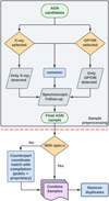 |
Fig. 1 Flowchart depicting the training sample down-selection pipeline. This includes the sample preprocessing (grey box) and the sample refinement, including redshift extension and duplicate removal below the dashed red line. |
2 AGN training sample selection
In X-ray surveys, the identification of AGN has two distinct advantages - (i) the reduced impact of moderate obscuration and (ii) the lack of host dilution. Due to the inherent brightness of accreting SMBHs compared to their host galaxies, this results in a significantly higher nuclei-to-host emission ratio compared to observations in some of the neighbouring wavelength windows, such as UV-optical-NIR (Padovani et al. 2017). This naturally leads to a larger diversity of AGN observed by an X-ray telescope. That being said, surveys in the more accessible optical and NIR regime can increase the likelihood of detecting higher-ɀ, and in the case of MIR more heavily obscured AGN, compared to the soft X-ray bands.
ML approaches for photo-ɀ estimation in large surveys (e.g., Fotopoulou & Paltani 2018; Duncan 2022) typically classify objects into three broad categories: galaxies, quasars (QSOs), and stars, before computing photo-z. However, this classification is usually based on the optical properties and hence fails for obscured and/or lower-luminosity AGN. Since our goal is to improve on the quality of photo-z estimates for X-ray detected extragalactic sources, including type 2 AGN and low-redshift Seyfert 1 galaxies, generally, our training sample has to replicate this diversity. We achieve this by combining AGN selected across multiple wavelength bands.
As a starting point, we include the same X-ray samples used in Saxena et al. (2024), namely the latest version of the XMM catalog, 4XMM, which spans 19 years of observations made with XMM-Newton (Webb et al. 2020) and data from the eROSITA CalPV-phase Final Equatorial-Depth Survey (eFEDS; Brunner et al. 2022), as they provide a reasonably representative and complete set of diverse AGN spanning five dex in X-ray flux out to redshift ɀ ≲ 4. However, with just these, some portions of AGN parameter space remain imbalanced, such as highly luminious and/or high-z AGN. Thus, we expand the dataset by adding bright, optical and MIR, selections. We describe each of these samples in more detail below.
This approach enhances the completeness of our training sample, which is essential to mitigate covariate shift, that is the shift in parameter space between the training and validation samples, so that the model generalizes effectively to new data (Norris et al. 2019). Subsequently, a non-representative training sample may lead to systematically biased outcomes (Newman & Gruen 2022). Accordingly, algorithms will be strongly weighted towards the most densely populated regions of the training space (Duncan 2022).
2.1 Beyond eFEDS and 4XMM
We can enhance the redshift distribution within our sample, particularly towards high (ɀ ≥ 3) redshift, in this otherwise underrepresented parameter space due to observational selection effects. We recognize the subsequent incorporation of unavoidable selection biases in each survey while restricting the inclusion of sources at low redshift to a minimum. While the balance between dataset quality and size is critical, deep learning algorithms that operate on pixel-level inputs tend to perform optimally only when training datasets contain ≥400 000 galaxy images (Schuldt et al. 2021; Dey et al. 2022a; Newman & Gruen 2022). Since our method would benefit from a larger sample (see Table 1), we chose not to apply stringent quality criteria by only considering high-quality data, significantly reducing the number of sources available training. Such a reduction would also prevent the model from learning to handle lower-quality data, limiting its application to only high-quality validation data. By not making an initial down-selection, we retain the flexibility to apply quality cuts to future blind samples by using LS10 flags later.
Overview of the relative fractions of source catalogs used in compiling our AGN training sample.
2.1.1 Samples from optical selection
We include the 2dF QSO Redshift Survey (2QZ, Croom et al. 2004) with ∼23 k color selected QSOs in the magnitude range 18.25 ≤ bJ ≤ 20.85 at redshifts lower than ɀ ∼ 3 and the QUasars as BRIght beacons for Cosmology in the Southern hemisphere survey (QUBRICS, Boutsia et al. 2020) with 224 bright (i ≤ 18) QSOs at redshifts of ɀ ≥ 2.5.
2.1.2 Samples from optical follow-up of X-ray sources
Additionally, we incorporate the SDSS-IV (Blanton et al. 2017) quasar catalog from Data Release 16 (DR16Q, Lyke et al. 2020) with ∼150 k quasars collected from various subprogrammes including optical/IR selection down to g ≤ 22 in the LS10 footprint after subselecting high quality spec-ɀ, as well as follow-up of X-ray sources from ROSAT (Voges et al. 1999; Boller et al. 2016; Salvato et al. 2018) and XMM (e.g. LaMassa et al. 2019). As successor science programme, we also consider the Black Hole Mapper (BHM) SPectroscopic IDentfication of ERosita Sources (SPIDERS, Anderson et al., in prep., Aydar et al., in prep.) from SDSS-V (Kollmeier et al., in prep) Data Release 18 (Dwelly et al. 2017; Coffey et al. 2019; Comparat et al. 2020; Almeida et al. 2023).
2.1.3 Samples of high-z sources
Given the strong imbalance above ɀ ∼ 3.5, we also include 400 optically/IR selected quasars at redshifts 4.8 ≤ ɀ ≤ 6.6 down to g ≤ 24 from the high-redshift quasar survey in the DESI Early Data Release (EDR, Yang et al. 2023) and a compilation of high-z quasars at ɀ ≥ 5.3 published in literature (Fan et al. 2022).
2.2 Spectroscopic cross-referencing
The parent sample of AGN is annotated with spec-ɀ, where available. According to Figure 1, we also consider sources, including those from eFEDS and 4XMM, with spatial counterparts from a compilation of public redshifts (Kluge et al. 2024). The procedure by which we match optical counterparts in our combined sample to a compilation of quality criteria down-selected spec-ɀ, is outlined in Sect. 3.1 of Saxena et al. (2024). Due to overlaps between surveys, we remove duplicates when combining samples. The final sample of sources with spec-ɀ comprises 40 489 objects, with a breakdown in Table 1. Correspondingly, the (cumulative) histograms illustrating the n(ɀ) distributions that collectively constitute the PICZL sample are presented in Figure 2.
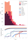 |
Fig. 2 Binned redshift histogram (top panel) and cumulative distribution (bottom panel) of the sources utilized in the PICZL AGN sample. Note that these samples are not necessarily rank ordered by importance but for improved readability. |
3 The survey
To streamline and simplify our methodology, we have chosen to employ data from LS10 exclusively to mitigate potential complications arising from the heterogeneity of multiple datasets. Crucially, the survey area now extends over 20 000 deg2 of optical ɡriɀ and WISE W 1 − W4 forced photometry, by incorporating the following datasets:
DECam Legacy Survey observations (DECaLS, Flaugher et al. 2015; Dey et al. 2019), including data from the Dark Energy Survey (DES, Dark Energy Survey Collaboration 2016), which covers a 5000 deg2 contiguous area in the South Galactic Cap. In the DES area, the depth reached is higher than elsewhere in the footprint.
DECam observations from a range of non-DECaLS surveys, including the full six years of the Dark Energy Survey, publicly released DECam imaging (NOIRLab Archive) from other projects, including the DECam Local Volume Exploration Survey (DELVE, Drlica-Wagner et al. 2021) and the DECam eROSITA survey (DeROSITAs, PI: A. Zenteno, Zenteno et al., in prep.).
In the north (δ > 32.375 deg), LS10 uses the Beijing-Arizona Sky Survey (BASS, Zou et al. 2017) for ɡ- and r-band coverage, and the Mayall ɀ-band Legacy Survey (MzLS, Silva et al. 2016) for ɀ-band coverage (Kluge et al. 2024).
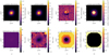 |
Fig. 3 Grid of subplots showing various model inputs for PICZL. In the upper row: the LS10 ɡ-band image (a), along with its 2-D model flux (b), residual (c), and aperture flux map (d). In the bottom row: the original g-r color is shown in (a). The presence of a saturated pixel in the top right corner is visible, indicating the need for pre-processing. The result of the preprocessing is shown in b. The bottom panels c and d show the ɡ/r-band and w1/w2-band aperture flux maps, respectively. |
3.1 Photometric data
LS10 offers registered, background-subtracted, and photometrically calibrated point spread function (PSF)-forced photometry, including corresponding errors. To extend their wavelength coverage, DR10 catalogs incorporate mid-infrared (mid-IR) forced photometry at wavelengths of 3.4, 4.6, 12, and 22 µm (referred to as W1, W2, W3, and W4, respectively) for all optically detected sources in the LS10 via the Near-Earth Object Wide- field Infrared Survey Explorer (NEOWISE) (Mainzer et al. 2011; Lang 2014; Meisner et al. 2017). Sources are modeled simultaneously across all optical bands, ensuring consistency in shape and size measurements by fitting a set of light profiles, even for spatially extended sources. Consequently, alongside reliable total and multi-aperture (eight annuli < seven arcseconds, five annuli <11 arcseconds for the optical and mid-infrared bands, respectively) flux measurements, the LS10 catalog offers seeing- convolved PSF, de Vaucouleurs, exponential disk, or composite de Vaucouleurs + exponential disk models obtained with the Tractor algorithm (Lang et al. 2016). Additionally, providing fluxes rather than magnitudes, enables considering sources with very low signal-to-noise ratios without introducing biases at faint levels. This characteristic also facilitates flux stacking at the catalog level, enhancing the overall versatility and utility of the classification and fitting process within LS102.
3.2 Imaging data
In addition to catalog data, LS10 provides a rich set of imaging products. These include observations, flux model images, and residual maps for all available bands. For instance, the top panels (a, b, c) of Figure 3 display all image products for a ɡ-band observation, respectively.
4 Preprocessing
Here we detail the preprocessing steps taken to prepare our dataset, ensuring that it is clean, normalized, and structured appropriately.
4.1 Image preprocessing
Building on the approach of Saxena et al. (2024), which demonstrated significant improvements by shifting from total to aperture flux utilizing information on the 2D light distribution, we aim to further refine the spatial characterization of sources. This is achieved by incorporating pixel-level flux resolution through imaging as base input. Images in individual bands or in combination (i.e., colors) reflect the surface brightness, angular size, and sub-component structures of the sources, indirectly providing redshift information (Stabenau et al. 2008). To obtain reliable photo-z directly from images, we utilize flux-calibrated optical cutouts across as many filters as available.
With an average seeing FWHM of 1.3 arcseconds under nominal conditions, LS10 provides a pixel resolution of 0.262 arcseconds per pixel for the optical bands, reaching depths between 23 and 24.7 AB, depending on the specific band and region of the sky (see Dey et al. (2019) and Figure 1 in Saxena et al. (2024)). To enhance computational efficiency and mitigate contamination from nearby sources, we restrict our cutout dimensions to 23×23 pixel, centered on the AGN coordinates in the four ɡriɀ LS10 bands. Our cutouts correspond to a field of view (FOV) of approximately 6 arcseconds × 6 arcseconds. We base our choice of FOV on the angular size-redshift relation by computing the angular diameter distance dΛ via:
 (1)
(1)
Equation (1) and Figure 4 elucidate the connection between an object’s physical size, its angular size, and redshift. Notably, we can effectively map galaxies with a diameter of 30 kpc – representative of main sequence galaxies (Wuyts et al. 2011) – within the confines of a 23×23 pixel cutout, covering the range of 0.5 ≤ ɀ ≤ 7.7.
Given that the FWHM of the W1, W2, and W3 images is six arcseconds, and of 12 arcseconds for W4, WISE band cutouts do not provide meaningful spatial information at this scale (see Figure 5). Therefore, we have opted to use images solely from the optical bands. Problematic sources, exhibiting signs of defects in various ways are flagged in the Legacy Survey by specific bitmasks (Dey et al. 2019).
We acknowledge that LS10 images exhibit varying quality due to differences in seeing conditions during observations taken over many years, which impact in particular the measurements of color within source apertures. Despite this, we rely on the model’s ability to adapt to these intrinsic variations given the size and diversity of our training sample, as the sources withheld from training represent a shuffled subsample of the main dataset, ensuring robust evaluation. We have verified that the distribution in seeing quality (expressed as the weighted average PSF FWHM of the images) for the training and validation are comparable (refer to Figure B.1). However, preliminary tests indicate that adding PSF size and PSF depth of the observations – both available in LS10 – as additional features enhances model performance (Götzenberger et al., in prep.). While it is not unreasonable to expect the model to implicitly infer the PSF or a related abstract representation thereof from the images themselves, these features will be included by default in future PICZL versions. With ongoing developments, PSF cutouts are expected to become more accessible for integration into the image stack (see Table 2). In the longer term, we anticipate that upcoming surveys like LSST, with their improved consistency in image quality, will further reduce these limitations and boost the precision of pixel-based analyses such as ours.
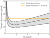 |
Fig. 4 Angular size of sources with a fixed physical size of 20–40 kpc, as a function of redshift. The orange dashed line depicts a fixed image dimension of 23 pixels, assuming the LS10 spatial resolution of 0.262 arc seconds per pixel, which suffices to cover objects of 30 kpc diameters in size out to redshifts of ~ 0.3 ≤ ɀ ≤ 7.8. |
4.2 Color images
It proves advantageous to provide the network with color images (ratio between images from different bands) as an additional input. This approach avoids the necessity for the model to learn the significance of colors solely from the flux images, which is inherently a more difficult task. Likewise, rather than processing numerical features separately and merging them with the information extracted from the image cube at a later stage, we find it beneficial to integrate them directly at the pixel level. As a result, whenever possible, we transform catalog features into 2D arrays to align them with the original images in the same thread, enabling smoother integration and more coherent analysis (see e.g. Hayat et al. 2021). We improve the depth of our data cube by converting catalog-based quantities, for example, flux measurements from apertures across different bands, into synthetic images, with a respective image size depending on the cutout size (see Figure 3). We expand this approach by generating images for all viable color combinations of aperture fluxes, constrained to those with matching aperture sizes. Additionally, we produce color images for flux cutouts where pixel resolutions are consistent (see lower panels b and c of Figure 3). Since the WISE and optical bands differ in both aperture size and pixel resolution, cross-wavelength color images are not feasible; instead, color combinations are restricted to within the optical or within the WISE bands (refer to Table 2).
To maintain FOV consistency, we integrate WISE data for only the two innermost apertures (see Figure 5), preserving the 23x23 pixel data cube format. Although no additional spatial details are expected at this scale (see Sect. 4.1), the WISE data still captures aperture flux in a format that enables direct crosschannel connections between optical and mid-infrared data at the image level.
Nevertheless, defected images can introduce challenges when generating color images (see bottom panel a) in Figure 3). Given that colors are derived from the ratio of images in different bands, the occurrence of unphysical negative or abnormally high/low values poses a significant concern. To address this issue, we examine whether the median value of neighbouring pixels is more than three times lower than the value of noisy pixels per band. If so, the central pixel’s value is substituted with the median value of the surrounding pixels to smooth out fluctuations. In cases of non-detections or severely corrupted images where the largest value among all pixels in an image is <0.001, the image is treated as a non-detection and all pixels are set to zero as default. After undergoing preprocessing, the images are utilized to create color images by exploring the six possible color combinations: ɡr, ɡi, ɡɀ, ri, rɀ and iɀ. If either of the two flux images involved in creating a color image is identified as a non-detection, the resulting color image is set to a default value of −99.
At the catalog level, spatially invariant features, such as best- fit model classifications and signal-to-noise ratios (S/N), are processed separately in a dedicated channel, as they cannot be converted into image data. Notably, regarding normalization, we adopt a uniform min-max scaling approach to handle columns with cross-dependencies, such as flux bands. This strategy aims to preserve crucial information, such as the original shape of the SED.
Contrary to the conventional approach of stacking all available images into a single input (Hoyle 2016; D’Isanto & Polsterer 2018; Pasquet et al. 2018; Dey et al. 2022a; Treyer et al. 2023), we find it advantageous to separate the color image data cube (23,23,24) from the flux band cutouts (23,23,32). This distinction is necessary because the color images often have differing pixel value scales, including negative values, which require specialized processing in our machine learning application, such as tailored loss functions in the CNN. Non-spatial attributes are then combined with image-based data at a subsequent stage of the model, allowing the model to capture both spatial and non- spatial aspects. By processing data types in parallel channels, we leverage their complementary information by merging the data at a later stage, enhancing the extraction of inter-band correlations and ultimately improving redshift precision (Ma et al. 2015; Ait-Ouahmed et al. 2023). A detailed breakdown of the features integrated into each channel is provided in Table 2.
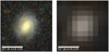 |
Fig. 5 Example AGN in our sample, as seen by LS10, in the optical RGB image (left) and in the W1 image from NEOWISE7 (right). The spatial resolution is 0.262 arcseconds and 2.75 arcseconds per pixel, respectively. The size of the cutouts is 27.5 arc seconds × 27.5 arc seconds. |
Overview of the various feature formats and dimensions utilized in PICZL’s multi-channel approach.
5 Neural network
ML embodies an artificial intelligence paradigm where computers learn patterns and relationships from data, enabling them to make predictions or perform tasks without explicit programming. Multilayer perceptrons (MLPs), a feature-based feedforward neural network, draw inspiration from their biological counterparts, namely excitable cells responsible for processing and transmitting information (Rosenblatt 1958; Goodfellow et al. 2016; Deru & Ndiaye 2019). Likewise, each assigned a distinct weight, computational input vectors can be organized into layers, relayed to one or more hidden layers, to compute a scalar output value (Géron 2019). During training, these models learn data mappings by adjusting the weights and biases associated with their connections. The margin of change to the model after every training epoch is dictated by the choice of optimizer and loss function, which effectively calculates the Euclidean distance between the prediction and so-called ground truth in multi-dimensional feature space, thereby significantly impacting model convergence and performance.
The current state-of-the-art deep learning (DL) networks, characterized by their many hidden layers, have shown exceptional capabilities in handling complex non-linear tasks.
5.1 Convolutional model layers
Among such architectures, Convolutional Neural Networks (CNNs; Fukushima 1980; LeCun et al. 1989; Lecun et al. 1998) distinguish themselves by their remarkable effectiveness in handling grid-like data, a prevalent form of which is represented by images. CNNs leverage a model architecture that is particularly effective in tasks like image recognition, object detection, and image segmentation (O’Shea & Nash 2015; Liu et al. 2022). In convolutional layers, neurons establish connections exclusively with pixels within their receptive field, ensuring successive layers are linked only to specific regions of the previous layer. Subsequently, the model extracts low, image-level features in early layers and progressively complex, higher-level features in later layers. This allows the CNN to learn representations of the input data at multiple levels of abstraction.
The convolutional operation involves sliding several kernels K, here of sizes 3×3 or 5×5 pixel, across the images with a fixed stride of size s = 1, compressing each mosaic element into a single scalar. This process entails element-wise multiplication, generating a set of K feature maps. Filters, the learnable parameters of convolutional layers, enable the network to detect and highlight different aspects of the input data, such as edges or corners. Each convolution is followed by a pooling layer that reduces spatial dimensions and computational load. Pooling involves sliding a kernel, in our case of size 2 × 2 and s = 1, across the feature maps, selecting the maximum value (max pooling) within each kernel window. After flattening the data cube into a single array, it is passed through (several) fully connected (FC) layers. Each FC layer contains a layer-specific number of neurons n, tailored to the model’s specific needs. The final FC layer’s neuron count varies based on the task, with n = 1 referring to regression tasks and n ≥ 2 to other endeavors such as multi-label classification.
5.2 Gaussian mixture models
By default, single output regression models (Schuldt et al. 2021) provide point estimates without quantifying uncertainty. This severely limits their area of application, particularly in scenarios where quantifying the uncertainty is crucial, for example, when performing precision cosmology with Euclid (Bordoloi et al. 2010; Scaramella et al. 2022; Newman & Gruen 2022). By instead employing an architecture that provides PDFs, we can not only retrieve point estimates but also encapsulate the uncertainty associated with the predictions in a concise format (D’Isanto & Polsterer 2018). Given the inherent complexity in determining redshifts from only a few broadband cutouts, our results are expected to often exhibit degeneracy with multi-modal posteriors, making a single Gaussian insufficient for representing the photo-ɀ PDFs. Therefore, estimates are computed using Bayesian Gaussian Mixture Models (GMMs, Duda et al. 1973; Viroli & McLachlan 2017; Hatfield et al. 2020). These networks provide a unique probabilistic modeling approach that differentiates them from traditional MLPs. One of the key distinctions lies in the output nature, where GMMs provide a set of variables to compute weighted multi-Gaussian distributions as opposed to single-point estimates. Subsequently, each component is characterized by its mean µ, standard deviation σ, and weight w, allowing GMMs to produce a full PDF for a given set of inputs x. The PDF is expressed as
 (2)
(2)
with, wk representing the weight and  denoting the Gaussian distribution of the k-th component. As such, we extend our CNN approach by a GMM backend to output PDFs based on the information-rich feature maps produced during the front-end phase of the network. However, we encounter a limiting challenge with inputs of such small dimensions, that is 23 × 23, as they are not well-suited for established image-based Deep Learning architectures, such as “ResNet” (He et al. 2015), which typically require larger dimension scales, typically exceeding 200 × 200 pixels, to accommodate the large number of pooling layers they employ. Therefore, we developed a custom architecture to fit our data dimensionality. The resulting model architecture features roughly 490 000 trainable parameters, far fewer than found in comparable studies (see Pasquet et al. 2018; Treyer et al. 2023), and is displayed in Figure A.1.
5.3 Model refinement
Numerous hyper-parameters are crucial in shaping the network architecture while influencing training and convergence. Extensive optimization has been conducted across various parameters utilizing the Optuna framework (Akiba et al. 2019). The current configuration accounts for the vast array of potential combinations. The key parameters with the most significant impact are outlined below:
Batch size [8–2048]: the number of objects utilized in a single training iteration per epoch. Larger batch sizes offer computational efficiency, while smaller batches may help generalize better.
Learning rate [0.1–0.00001]: controls the size of the model adjustment step during optimization. It influences the convergence speed and the risk of overshooting optimal settings.
Number of Gaussians [1–50]: determines the complexity and flexibility of the GMM, influencing how well the model captures the underlying data distribution.
Convolutional & pooling layers [2–10]: the dimension of the kernel influences the size of the receptive field and the learnable features.
Number of neurons and layers [10–300]: determines the depth and complexity of the neural network, impacting its capacity to capture hierarchical features and relationships in the input data.
Activation function: introduces non-linearity to the model, enabling it to learn complex mappings between inputs and outputs, commonly a sigmoid, hyperbolic tangent (tanh), rectified linear unit (ReLu) or versions thereof.
Dropout layer [0–0.9]: refers to the fraction of randomly selected neurons that are temporarily dropped or ignored during training, helping to prevent overfitting by enhancing network robustness and generalization.
Max and average pooling: pooling layers, such as Max Pooling and Average Pooling, are used to downsample the spatial dimensions of the input feature maps, reducing the computational load.
Batch normalization: Batch Normalization can improve the training stability and speed of convergence in neural networks by subtracting the batch mean and dividing by the batch standard deviation.
5.4 Loss functions
When utilizing PDFs instead of point estimates, it is crucial to quantify whether a predicted PDF effectively reflects the ground truth, in our supervised ML case, spec-ɀ (Sánchez et al. 2014; Malz et al. 2018; Schmidt et al. 2020; Treyer et al. 2023). The PDF predicted by a model should be concentrated near the true value. A straight-forward and meaningful proper scoring rule (i.e. one which is lowest when the prediction is at the truth), is the product of probabilities at the true redshifts. The negative log-likelihood (NLL)3 of which passed to a minimizer
 (3)
(3)
yields the likelihood of observing a data distribution given a specific set of model parameters. This expression coincides with the average Kullback-Leibler divergence (KL, Kullback & Leibler 1951) when going from a delta PDF at spec-ɀ to the photo-z PDF.
An alternative growing in popularity is given by the Continuous Ranked Probability Score (CRPS), initially applied in weather forecasting (Grimit et al. 2006), which serves as a valuable metric for photo-z estimation via PDF quantification (D’Isanto & Polsterer 2018). Computationally, CRPS calculates the integral of the squared difference between the predicted cumulative probability distribution function (CDF) and a Heaviside step-function H(x) at the value of the spec-ɀ (xɀ) as
![Mathematical equation: ${\mathop{\rm CRPS}\nolimits} \left( {F,{x_z}} \right) = \int_{ - \infty }^\infty {{{\left[ {\int_{ - \infty }^x f (t){\rm{d}}t - H\left( {x - {x_z}} \right)} \right]}^2}} {\rm{d}}x.$](/articles/aa/full_html/2024/12/aa52361-24/aa52361-24-eq5.png) (4)
(4)
For a finite mixture of normal distributions M, the CRPS can be expressed in closed form:
 (5)
(5)
with δi = y − µi, the uncertainty σi and weight wi of the i-th component respectively, as well as
![Mathematical equation: $\eqalign{ & A\left( {\mu ,{\sigma ^2}} \right) = \mu \left[ {2\Phi \left( {{\mu \over \sigma }} \right) - 1} \right] + 2\sigma \phi \left( {{\mu \over \sigma }} \right), \cr & \,\,\,\,\,\,\,\,\,\,\,\,\,\,\,\phi (x) = {1 \over {\sqrt {2\pi } }}\exp \left( { - {{{x^2}} \over 2}} \right), \cr & \,\,\,\,\,\,\,\,\,\,\,\,\,\,\,\,\Phi (x) = \int_{ - \infty }^x \phi (t){\rm{d}}t. \cr} $](/articles/aa/full_html/2024/12/aa52361-24/aa52361-24-eq7.png) (6)
(6)
By extending the CRPS loss via normalizing it by (1+z), we adjust the penalty for prediction errors based on redshift. In doing so, we prioritize accuracy for low and intermediate redshift sources by imposing higher constraints while allowing for more leniency in less critical high-redshift areas. Integrating over the entire range of possible redshift values, the CRPS takes into account both location and spread of the predicted PDF. It, therefore, provides a comprehensive evaluation metric, generating globally well-calibrated PDFs (Dey et al. 2022b).
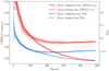 |
Fig. 6 Training (dashed) and Validation (solid) loss curves for a single PICZL model. The solid or dashed lines represent the mean loss values computed over a window size of 20, while the shaded areas denote the 1σ error range around the mean. The NLL loss is depicted in blue, while the normalized CRPS loss is shown in red. |
5.5 Training and data augmentation
Our dataset is divided into training and validation sets in an 80:20 ratio. The model is trained over 1000 training epochs utilizing the Adam algorithm (Kingma & Ba 2017) along with a learning rate scheduler to adjust the learning rates during training dynamically. The inclusion of both is a consequence of the Optuna hyperparameter optimization. Typically, the model achieves its lowest validation loss around the 600th epoch when considering both loss functions (see Figure 6). After this point, although the training loss continues to decrease, the validation loss begins to increase, indicating overfitting. This overfitting likely arises due to the limited size of our training sample, allowing the model to memorize specific patterns rather than learning generalizable features. We implement a checkpoint system to mitigate this, saving the model’s architecture and parameters when it reaches its lowest validation loss. This approach ensures that we capture the best-performing model configuration while preventing overfitting.
To further exploit the advantages of deep learning, particularly its capacity to perform well with extensive datasets, we have tested the incorporation of data augmentation techniques into our methodology. Recognizing the substantial impact of training data amount on model performance, we employ common augmentation data products, such as rotated and mirrored images. Although these transformations significantly increase the apparent size of the dataset, we do not observe an increase in performance when including augmentation techniques (Dey et al. 2022a; Treyer et al. 2023). This is potentially not surprising as the influence of augmentation techniques depends on several factors. While CNNs are inherently equivariant to translations within images, enabling them to recognize objects even if they are shifted or off-centered, they and most other machine-learning approaches are not naturally equivariant to rotations and reflections. This lack of rotational equivariance means that the model output effectively depends on the rotation of the input images. However, as most of our inputs are approximately point sources with radial symmetry, we do not explore this aspect further in this study. More recent publications have focused on developing rotationally equivariant CNN architectures, which have shown improved performance despite increased computational costs (Cohen & Welling 2016; Weiler & Cesa 2021; Lines et al. 2024). Incorporating such architectures could be particularly beneficial for future works dealing with large amounts of imaging data.
5.6 Model ensemble
Ensemble models capitalize on the diversity of multiple models to improve prediction accuracy. Our approach involves diversifying models by adjusting parameters such as the number of Gaussians per GMM, learning rates, batch sizes, and the choice of loss function. We employ both NLL and CRPS as complementary loss functions to achieve this. While CRPS excels in achieving lower outlier fractions, NLL enhances overall variance. Each loss function trains a set of 144 models, resulting in a diverse pool of 288. In line with Treyer et al. (2023), we achieve superior performance by randomly combining equally weighted CRPS and NLL models from the pool, compared to the bestperforming individual model (Dahlen et al. 2013; Newman & Gruen 2022). This finding is also aided by the result that roughly 30% of outliers are model-specific as opposed to 20% of outliers appearing in all models, therefore considered to be genuine. Put differently, 80% of outliers were found to not be an outlier in at least one other model.
We additionally recognize that the initial configuration of each model has a minor influence on the performance. Although training additional models could further enhance our results, the computational resources required to generate three to five sets of models would make this approach impractical relative to the potential performance gains. To create an effective ensemble, we evaluate the outlier fraction of all individual models on an unseen test sample. From this evaluation, we select models based on their relative influence on the model performance. We then observe how the ensemble’s performance evolves as more models are continuously incorporated. Our ensemble ultimately comprises 10 models or 84 Gaussians, evenly incorporating models optimized using both NLL and CRPS approaches. To refine the model weights within the ensemble, we employ Optuna for fine-tuning. Subsequently, the ensemble posterior likelihood distribution Pensemble (x) is given by:
 (7)
(7)
where the weights wi are normalized such that:
 (8)
(8)
to assure that the integral of the ensemble PDF is equal to 1. We obtain a point estimate for our photo-ɀ prediction by identifying the dominant mode of the resulting PDF, recognizing that the mean or median could be misleading for highly non-Gaussian and bi- or multi-modal distributions. Additionally, we provide asymmetric one and three σ upper and lower errors by evaluating the PDF within the 16th/84th and 0.15/99.85th percentiles, respectively, along with the entire PDF.
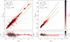 |
Fig. 7 Binned scatter plots of photo-z obtained from our model ZPICZL versus spectroscopic redshift Zspec , for sources classified as type point-like (PSF, left) and extended (EXT, right). Each plot includes identity and two lines denoting the outlier boundary of |

6 Photo-z results
We evaluate the performance of PICLZ on both point estimates and PDFs. This comprehensive assessment includes testing the statistical reliability and accuracy of our predictions. We adopt several commonly employed statistical metrics, providing insights into the accuracy, precision, and reliability of the photo- z estimates. In line with the definitions from the literature, we use the following metrics:
Prediction bias: the mean of the normalised residuals,
 .
.Variance: following Ilbert et al. (2006), we adopt the standard deviation from the normalised median absolute deviation
 .
.Fraction of outliers η is determined by the proportion of photo-z estimates with absolute normalised residuals exceeding
 .
.PIT score: a diagnostic tool used to evaluate the calibration of probabilistic forecasts by evaluating the cumulative distribution function (CDF) given the PDF at the (true) spec-z zcorr as
 .
.
We quantify PICZL’s performances on a validation sample of 8098 sources and find an outlier fraction η, of 5.6% with a variance σNMAD, of 0.045. Since the validation sample is used for feedback in training, it should be mentioned that the results mentioned above are likely overestimating the performance and therefore may not representative of what a future user could achieve with say, a test set previously unknown to the model, leave-one-out, or k-fold cross-validation. To this end, we have estimated our performance on independent, blind, X-ray-selected samples (see Sects. 6.2 and 7).
Figure 7 compares photometric versus spectroscopic redshifts, split by point-like (type=PSF) and extended (type=EXT) morphology. With respect to comparable work (e.g., Figure 13 from Salvato et al. 2022), we observe enhanced performance with a much-reduced fraction of outliers, especially for PSF sources. These objects lack morphological information at redshifts ɀ ≳ 1, hence we attribute this improvement to the model’s ability to recognise how the radial extension of the azimuth profile of sources changes with redshift (refer to Figure 4). The scatter, for both PSF and EXT distributions, is tight and symmetrically distributed around the ɀPICZL = ɀspec identity line, with outliers appearing randomly scattered, suggesting stable performance across the redshift range and minimal systematic errors (see Figure 8 and Dey et al. (2019) for reference).
Given that our point estimates are derived from PDFs, we must ensure their global calibration and accuracy. To achieve this, we employ the probability integral transform (PIT) statistic (Dawid 1984; Gneiting et al. 2005), a widely accepted method in the field for assessing the quality of redshift PDFs (Pasquet et al. 2018; Schuldt et al. 2021; Newman & Gruen 2022). An ideal scenario is represented by a uniformly distributed histogram of PIT values. Any deviation from uniformity can indicate issues in PDF calibration. Under-dispersion may suggest overly narrow PDFs, while over-dispersion often results from excessively wide PDFs (D’Isanto & Polsterer 2018). Peaks close to zero or one can be explained by catastrophic outliers, where the true redshift lies so far in the wing of the PDF that it essentially falls outside of it.
We employ the PIT histogram (top panel Figure 9) alongside quantile-quantile (QQ) plots (bottom panel Figure 9), to visually assess the statistical properties of our model predictions. For reference, these can be compared to Figure 2 of in Schmidt et al. (2020); however, those code performances are completely dominated by inactive galaxies, making a direct comparison impractical. The QQ plot compares the CDFs of observed PIT values and identity U(0,1), to visualize QQ differences split by morphological type.
A well-calibrated model will exhibit a QQ plot closely following identity with a flat PIT histogram, indicating accurate and reliable redshift predictions. Our analysis shows that, while asymmetry in the PIT distribution could suggest systematic bias, the QQ plot reveals small residuals overall. Notably, for both the single- (refer to Sect. 5.2 and Figure A.1) and ensemble model (refer to Sect. 5.6), the curves do not deviate significantly from zero, lesser so for PSF-type than EXT-type objects, indicating well-calibrated models. A distinct observation is the shift towards central PIT values for the ensemble model. This shift is not unexpected, given that the ensemble approach integrates multiple redshift solutions, each potentially contributing different peaks to the resulting ensemble PDF. Consequently, the ensemble PDF exhibits a broader bulk of probability across redshift, with PIT scores accumulating more area under the curve when integrated to the main mode. As a result, rather than yielding a flat PIT distribution, the histogram shifts towards having a concentration of values around 0.5. While this phenomenon aligns with our expectations, further enhancements may be realized by incorporating metrics tailored instead to local calibration accounting for population-specific subgroups (see e.g. Zhao et al. 2021; Dey et al. 2022b).
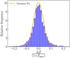 |
Fig. 8 Histogram distribution of the normalised residuals, overlaid with a Gaussian fit (orange). The parameters of the Gaussian distribution are determined by the prediction bias and σNMAD values obtained from Table 5 for the validation sample. |
6.1 Model performance for different inputs
Images provide a more comprehensive view of astronomical sources by capturing their full spatial structure and light distribution, offering finer details on morphology, apparent size and extended features that are often lost in the averaging process of aperture photometry. This is pivotal, as SED features crucial for determining redshift solutions and resolving degeneracies mostly reside within the host galaxy (Soo et al. 2017; Wilson et al. 2020). In particular for AGN, images help to spatially separate the pixels corresponding to AGN-dominated emission and those corresponding mostly to the host galaxies. This approach enhances our ability to isolate and analyze individual pixel strings across multiple filters, to effectively construct SEDs for the host galaxies independently. We thereby capture subtle features, neighbors, and patterns that may not be discernible from total flux measures. Critically, the independent photo-z from the AGN and host must agree, thus narrowing the overall source PDF.
Table 3 presents the fraction of outliers for both EXT and PSF sources using different configurations of the PICZL algorithm. The first setup replicates the feature-only method, relying solely on total fluxes from the catalog, which, as seen in other studies, results in the fraction of outliers for PSF sources being nearly three times higher than for EXT sources (Salvato et al. 2022). In the second configuration, we adopt the approach of Saxena et al. (2024), incorporating the 2D light distribution and color gradients within annuli. The third configuration, that is PICZL as outlined above, enhances this by incorporating images, supplemented with catalog values transformed into image format, which leads to an additional improvement over the method in Saxena et al. (2024).
Since images inherently capture all features typically extracted numerically and presented in catalogs, we show in the fourth case that PICZL achieves excellent results without feature/catalog information, using solely optical images supplemented by WISE aperture flux maps, even without explicit hyperparameter tuning. This approach is particularly promising for future surveys such as LSST and Euclid, where relying solely on multi-band imaging, including NIR/IR, will eliminate the need for complex source modeling or aperture photometry, regardless of the sources being galaxies or AGN.
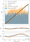 |
Fig. 9 Display of the QQ plot, comparing identity (flat histogram) against the PIT values derived from our redshift PDFs of the validation sample (top panel), and the differences between the QQ plot and identity, highlighting systematic biases or trends for the two morphological classes (PSF and EXT), shown in the bottom panel. For all panels, blue refers to results achieved with a single model (see Figure A.1) while orange reflects the results obtained when utilizing ensemble results (refer to Sect. 5.6). |
6.2 Blind sample comparison
To evaluate the robustness of our approach, we tested PICZL on an independent blind sample from the Chandra Source Catalog 2 (CSC24). This sample, selected to ensure no overlap with the training data, but yield a comparable X-ray to MIR distribution, is the same one used in the CIRCLEZ analysis (Saxena et al. 2024), allowing for a direct comparison with their results. After filtering for sources with spectroscopic redshift and removing duplicates with the training dataset, the sample comprises 416 sources within the LS10-South area. For comparison, Saxena et al. (2024) achieve an outlier fraction, η, of 12.3% and a normalized median absolute deviation, σNMAD, of 0.055, while our algorithm yields a superior σNMAD of 0.046 and η of 8.3% (see Sect. 8.6.2 and Figure C.1). This comparison, therefore, demonstrates how utilizing image cubes further improves the already good results achieved using 2D-information from a catalog. For more details on the sample, see Saxena et al. (2024).
6.3 Prediction uncertainty quantification
Accurate error estimation is crucial for assessing the reliability of any prediction, particularly in those astrophysical contexts where uncertainties can significantly impact the interpretation of data. To this end, we provide asymmetrical 1σ and 3σ errors for every source, together with the photo-ɀ PDF, as detailed in Sect. 5.6. These error estimates offer a comprehensive understanding of the potential variance in our predictions, accurately reflecting the inherent uncertainties in our data and model. We include asymmetrical errors, as the true distribution of uncertainties is often not symmetrical. This asymmetry arises from factors such as photometric noise and degeneracies in the highly non-linear color-redshift space, where certain higher or lower redshift values may be more probable than their counterparts, leading to skewed PDFs. Although symmetrical redshift errors are observed for the majority of sources, approximately one-third of the sources exhibit asymmetrical 1σ errors with deviations in redshift up to |∆ɀasym| ≃ 0.25.
Figure 10 displays PICZL point estimates as a function of PDF width, represented by the upper 1σ minus lower 1σ, color-coded by the Legacy Survey r-band magnitude, as it offers the most extensive coverage compared to the g, i, or ɀ bands, containing the largest number of sources. We observe wider PDFs correlating with higher redshifts and fainter sources characterized by higher photometric errors or lower S/N, as discussed in Sect. 8.4. Additionally, the widths of the PDFs exhibit noticeable horizontal structures, largely influenced by the nature of the LS10 filters. We find that PDFs with wider modes, indicating less certain redshift estimates, often correspond to redshift ranges where key spectral features, such as the Ca break, fall outside the filter coverage (e.g. ɡ&r at ɀ ≃ 0.4, r&i at ɀ ≃ 0.8 and ɀ ≃ 1.5 or ɀ ≃ 2.2). At redshifts approaching ɀ ≈ 3 and extending below ɀ ≈ 5, the Lyman-α break starts to fall within the filter ranges, which contributes to narrower PDFs with increased PDF width only observed for extremely faint sources at even higher redshifts. Lastly, we find that the number of sources with wider PDFs increases as a function of  , indicating that narrower PDFs correspond to more accurate point predictions.
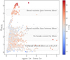 |
Fig. 10 PICZL point estimates as a function of PDF width, represented by the difference between upper and lower 1σ values. Each data point is color-coded according to its r-band magnitude from the LS10. The tilt of the distribution traces the increased uncertainties for PDFs of fainter sources. Horizontal distributions represent areas of large uncertainty in the photo-z, indicating that PICZL errors are realistic. |
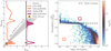 |
Fig. 11 Examples of an inlier (orange) and an outlier (purple) PDF (left panel). By definition, the point estimate derived for the two sources from the main mode falls within or outside the grey shaded region. Both sources show a secondary peak in the PDF. We can define the probability of being an inlier (colored area under the PDF which coincides with the grey shaded area). Normalized |

6.4 Insights from multimodal PDFs
To investigate whether predicted outliers are genuine anomalies or instead stem from machine learning processes, we inquire whether secondary peaks in PDFs are physically meaningful or training artifacts. For each source, we compute the fraction of its PDF, that satisfies the condition  , to provide , the probability of being considered an inlier. The left panel of Figure 11 illustrates this with examples of two PDFs (one for an inlier and one for an outlier), where we highlight the corresponding inlier probabilities. In the right panel of Figure 11, we plot
  re-normalised to scale [0,1], such that

as a function of inlier probability for all sources. The horizontal dashed black line separates the inliers (<0.5) from the outliers (≥0.5). The majority of inliers are concentrated at high inlier probabilities. This suggests that most inliers provide confident, unimodal PDFs with low errors. Likewise, most outliers have low inlier probability, with only a few outliers having more than 50% inlier probability. While this quantity cannot be computed for sources lacking spectroscopic redshift, it can be used to evaluate the reliability of our point estimates considering their associated PDFs.
To evaluate whether ensemble solutions with broad or complex distributions effectively capture the true redshift, we identify sources with multiple peaks and measure the proportion of PDFs exhibiting more than one mode. For these sources, we define a secondary peak as significant if it accounts for at least 10% of the height of the primary peak, which is the minimum prominence threshold used in our analysis. The top panel of Figure 12 shows that only 3% of inliers exhibit secondary peaks as opposed to the roughly 30% of outliers, where occurrences of strong secondary modes decrease with increasing prominence for both cases. While a single mode typically indicates a secure estimate for inliers, the presence of a unique mode alone can subsequently not be used to determine whether a source is an outlier.
Conversely, in the bottom panel of Figure 12, we present the recovery fraction, which denotes how often a secondary peak in PDFs exhibiting multi-modal distributions corresponds to the true redshift. Among the outliers with 30% multi-modal PDF, more than 70% have one of their secondary peaks corresponding to  , indicating that there is significant probability that the redshift could consequently be considered as an inlier if the peak heights were reversed. Given the PIT histograms shown in Figure 9, it appears likely that the PDFs are accurately capturing the relative frequency of multi-& bimodal PDFs, as if they were not, there would likely be bias evident in the overall PIT distribution. In other words, using this particular dataset, despite incorporating full multiwavelength image cutouts and catalog-level information, there persist areas of parameter space that are legitimately degenerate in redshift, and the PDF parameterization looks to be capturing that degeneracy accurately. Consequently, we recommend using the entire PDF rather than point estimates, when possible.
7 PICZL applied to other surveys
We want to investigate how PICZL, utilizing LS10 photometry and imaging, performs in determining photo-z for AGN in a more generic setting. Our focus is set on the LSST deep drilling fields (DDFs), selected to study SMBH growth across the full range of cosmic environments. These fields offer deeper, more comprehensive spectroscopic redshift coverage, along with a broader range of high-sensitivity bands, providing an enhanced dataset for photo-z estimation.
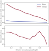 |
Fig. 12 Fraction of sources having a PDFs presenting secondary peaks for outliers (burgundy) and inliers (blue) are shown in the upper panel with corresponding recovery fraction for outliers (bottom panel). Both metrics are plotted as a function of the relative prominence threshold of the secondary peak. |
7.1 XMM-SERVS
The XMM-Spitzer Extragalactic Representative Volume Survey (XMM-SERVS, Mauduit et al. 2012) encompasses three key fields: the XMM-Large Scale Structure (LSS, Chen et al. 2018), spannning 5.3 deg2 with a flux limit of 6.5 × 10⁻¹⁵ erg cm−2 s−1 over 90% of the survey area in the 0.5–10keV band (Savić et al. 2023); the Wide Chandra Deep Field-South (W-CDF-S, Ni et al. 2021) and the European Large-Area ISO Survey-South 1 (ELAIS-S1, Ni et al. 2021), covering approximately 4.6 deg2 and 3.2 deg2 (Brandt et al. 2018; Scolnic et al. 2018), limited to 1.3 × 10⁻¹⁴ erg cm−2 s−1, respectively, each selected for their exceptional multiwavelength coverage and strategic alignment with the DDFs.
7.2 Photo-z computation
Considering that the original XMM-SERVS photo-z benefit from high S/N photometry and broader wavelength coverage, including u-band and NIR coverage, we would expect significantly better results compared to those achievable by PICZL using LS10 data alone. However, PICZL obtains comparable if not better results when limiting the sample to the depth at which it was trained on (see XMM-SERVS magnitude distribution in Figure E.1). Like any ML model, it struggles to extrapolate to faint sources outside its training distribution. Therefore, a fair comparison requires limiting the analysis to a similar feature space, while the results in Table 4 reflect performance across the entire, diverse XMM-SERVS samples. To facilitate a comparison with PICZL, our analysis begins with the counterpart associations of X-ray emissions as presented in Ni et al. (2021) and Chen et al. (2018). Whenever possible, we limit our samples to sources flagged as AGN (as defined in Sect. 6 of Ni et al. 2021). Matching to objects detected in LS10, due to its more limited depth, we identify approximately one-third of the original sources (see Table 4). This limitation is particularly pronounced in the XMM-LSS survey, where, in addition to deeper X-ray data corresponding to fainter counterparts, Chen et al. (2018) restrict their sample of AGN for which they calculate photo-z, to strictly non-broad-line X-ray sources. We select all sources with spectroscopic redshift and exclude those previously included in the PICZL training sample (see Table 4). Unlike the original works, PICZL also successfully computes photo- z for the significant fraction of sources for which the SED fitting adopted in XMM-SERVS failed (refer to w/photo-ɀS in Table 4). Figure 13 visualizes the outlier fractions (top) and variances (bottom) for the aggregate XMM-SERVS samples. Blue and burgundy represent the distributions including/excluding catastrophic failures in the XMM-SERVS catalogs. The plot is limited to outlier fractions of 30% and variances of 10%, as XMM- SERVS curves including zphot = −99 solutions continue to rise for fainter magnitudes or lower S/N. This suggests that, with increasing magnitude, a decreasing number of accurate estimates are available, making the subset excluding such solutions increasingly non-representative in terms of outlier fraction.
However, by limiting our comparison to sources with photo- z obtained from XMM-SERVS, we find that the accuracy of these photo-z remains comparable up to magnitudes around 23.5 AB, despite the more limited data being used. Additionally, we observe enhanced performance in PICZL photo-z for sources with S/N values ≳60, depending on the specific XMM-SERVS sample. Importantly, sources with S/N ≳ 10–20 mark a critical threshold range in LS10 where lower S/N values lead to an exponential rise in photometric errors (see Figure D.1). This trend is particularly evident for magnitudes fainter than 21.5 in the i-band (Saxena et al. 2024) and visible in all panels of Figure 13.
Figure 14 presents a visual comparison of normalized residuals for outliers identified by either PICZL or the original photo-z from Ni et al. (2021), exemplified via the ELAIS-S1 field. The spread of biases, excluding failures from XMM-SERVS, is similar for both methods, falling mostly within the range of [−0.5, 0.5]. The outliers in common appear to be modestly brighter than those that are outliers for a single method only and are evenly distributed between overestimation and underestimation. Notably, the outliers from Ni et al. (2021) are over a narrower range, while PICZL has a few brighter and several more fainter, the majority of which with magnitudes beyond the range covered during training. The observed difference in outlier rates, is not primarily due to the use of template-fitting versus machine-learning methods but rather a reflection of the available photometry. XMM-SERVS, with its deeper photometry, is well-suited for faint objects, though saturation in brighter sources may contribute to some outliers. PICZL, which leverages the LS10 dataset, is optimized for brighter sources due to the shallower photometry. While it performs well in this regime, fainter objects that fall outside the known parameter space are consequently less constrained.
8 Discussion
While Saxena et al. (2024) made significant strides in overcoming the limitations of relying solely on total or model fluxes for photo-ɀ estimation of AGN by utilizing all redshift-correlated features in the LS10 catalog, we have further advanced this approach. By integrating data from both optical and MIR wavelengths, our study highlights the transformative potential of combining imaging with catalog-level data. Despite the state-of-the-art advancements in photo-ɀ estimation for AGN in this work, further improvements will be possible only by solving issues related to data quality. By overcoming these issues, we can significantly reduce the fraction of catastrophic outliers and achieve even greater accuracy in our predictions. In the following, we discuss the limitations that need to addressed in order to apply PICZL to upcoming imaging surveys.
Summary of the XMM-SERVS samples and their respective photo-ɀ metrics.
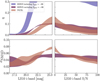 |
Fig. 13 Outlier fraction (top row) as a function of LS10 i-band magnitude (left) and LS10 i-band S/N (right), comparing the original photo-z from XMM-SERVS to the photo-z computed with PICZL. The XMM-SERVS photo-z results are shown both with and without the inclusion of sources for which XMM-SERVS photo-z failed (photo-z = −99). The shaded regions represent the range of XMM-SERVS outlier fractions across the ELAIS-S1, W-CDF-S, and LSS fields. The bottom row panels depict the range of XMM-SERVS variance in the three fields as a function of LS10 i-band magnitude and S/N. PICZL demonstrates a lower outlier fraction for brighter sources while maintaining comparable accuracy to the original photo-z estimates. Additionally, PICZL successfully computes photo-z for sources that are failures in the original methods. |
8.1 Incorrect spec-z
First and foremost, we need to address the reliability of the labels used in our, and generally any supervised machine learning algorithm. While spectroscopic redshift are typically trusted as accurate representations of true redshifts, this assumption does not always hold. As surveys continue to expand in scale, automated pipelines become indispensable for assigning spectroscopic redshift and identifying artifacts/problems for each source, as manual verification by visual inspection is impractical and will remain so for future surveys (Bolton et al. 2012). Importantly, most pipelines are trained on determining the redshift of the bulk of objects (Alexander et al. 2023), which are inactive galaxies and not AGN. This implies that a non-negligible fraction of AGN have wrong redshift estimates, including many labelled with “no warnings” (Hewett & Wild 2010; Wu & Shen 2022). Consequently, our performance is constrained by the unknown amount of incorrectly identified spectroscopic redshift per survey. While this fraction may be smaller for galaxies without nuclear activity, AGN present a range of challenges where pipelines fail. Examples of failures include cases where Mg-II is misidentified as Lyman-α for example, leading to ambiguous redshifts around ɀ = 0.7–0.9 ⇔ 1.5–2.5 or sources with strong featureless continuum typical of Blazars or, finally, sources with intense broad emission lines compared to the background continuum (Chen et al. 2018; Ni et al. 2021), as well as those with weak emission lines and a flat continuum background.
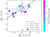 |
Fig. 14 Normalized residuals for PICZL photo-z compared to XMM-SERVS photo-z, using data from XMM-SERVS ELAIS-S1. PICZL outliers are shown as triangles, XMM-SERVS outliers as stars, and sources that are outliers in both methods are depicted as octagons. All sources are color-coded based on their LS10 i-band magnitude. |
8.2 Incorrect type classification
A subset of sources in the training sample, although having redshifts of ɀ ≥ 1, are classified as extended (i.e. non-PSF). This classification is likely incorrect, given the pixel resolution of LS 10. The apparent extension is more plausibly a result of poor seeing conditions that were not properly accounted for, or the presence of nearby neighboring sources (see Sect. 5.3 of Hsu et al. 2014). Since the morphological type affects predictions, akin to a prior in template fitting methods, this misclassification explains the increase in outliers within the EXT sample as redshift increases (see middle row in right panel of Figure 15). To verify this, we computed the absolute g magnitudes for outliers to assess whether their values fall within the expected range for galaxies and AGN (Véron-Cetty & Véron 2010). Figure 16 shows that 16% of sources classified as EXT (and thus galaxy dominated) have an absolute magnitude which exceeds the range typical of galaxies MEXT [−16,−24], confirming that their TYPE is wrongly assigned. Interestingly, approximately 96% of PSF sources meet the absolute magnitude requirement of MPSF [−20,−31], indicating that their TYPE is generally accurate.
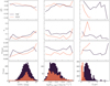 |
Fig. 15 Prediction bias (top row), fraction of outliers (second row), variance (third row), and number count (fourth row) as a function of magnitude (r-band from LS10), 0.2–2.3 keV X-ray flux, and spec-ɀ, categorized by type (extended (EXT)/point-like (PSF)). |
8.3 Faulty photometry
In addition to issues connected to the reliability of labels, predictions also face challenges due to data inconsistencies arising from faulty photometry. Surveys often flag issues of this kind directly, including problems such as hot pixels, saturation, cosmic rays, bleed trails, and other uncategorized anomalies. Detecting and addressing such observational defects is crucial because the accuracy and reliability of photo-ɀ predictions cannot be guaranteed for compromised photometric inputs. We experimented with removing various groups of sources affected by observational artefacts but found no improvement when excluding any single group. We therefore assume that, while removing some problematic sources could potentially improve performance, the reduction in training data size offsets any gains. Adding this kind of noise to the current training sample could be an approach to decouple these two effects. Consequently, we treat the inclusion of all problematic sources as natural noise, as opposed to artificially degrading images employing methods such as Gaussian noise (Hayat et al. 2021).
8.4 Survey depth
When splitting the validation sample by S/N across all bands, we find a higher outlier fraction in sources with low S/N (see Table 5). Consequently, to evaluate the reliability of our photo-ɀ, we need to consider the photometric depth of LS10 and how increased photometric errors for fainter sources impact redshift estimate uncertainties. Figure 15 presents the prediction bias 〈ɀ〉, outlier fraction η, and dispersion σNMAD as functions of r-band magnitude in LS10, X-ray flux (when available), and spec-ɀ. As the r-band magnitude increases, as expected, the outlier fraction and scatter rise. This pattern is consistent with the exponential increase in photometric errors for, e.g., i-band magnitudes ≳21.5, beyond which the outlier fraction, which otherwise remains well below 10%, and scatter also appears to rise, especially for sources of type EXT (refer to Figure D.1). While faint LS10 sources have unreliable photo-z, future surveys such as LSST and Euclid will probe deeper with improved S/N. As such, our methodology can be adapted to these next-generation surveys, ensuring high accuracy across a broader range of magnitudes and providing robust redshift estimates for the extensive AGN populations these and other surveys will detect.
Comparison of bias, fraction of outliers, and variance between photo-z computed with PICZL for various subsamples.
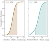 |
Fig. 16 Cumulative fraction of outliers as function of absolute magnitudes, to validate their classification based on TYPE. The left panel shows outliers classified as PSF, where most sources have absolute magnitudes consistent with AGN or QSO characteristics. In the right panel, 16% of EXT-classified outliers exhibit absolute magnitudes more typical of QSOs. |
8.5 Missing i-band
For DR10, the Legacy Survey footprint was extended by incorporating all available DECam data from various contributing surveys (refer to Sect. 3), including coverage in the i-band, though limited to a single pass. As a result, ~ 10% of sources lack i-band observations. Unsurprisingly, and as shown in Table 5, the accuracy of photo-z increases when this band is also available.
8.6 Biases
While the photo-z residuals exhibit a symmetric distribution around zero with minimal scatter, they do not consistently center at zero, suggesting a potential systematic bias in the photo-z estimates. Ideally, we would like to achieve normalized residuals that remain consistent irrespective of redshift or selection. Currently, this is not the case, as biases are not corrected for and are mostly influenced by the distribution of our training samples, which are specific to their respective survey and inherently biased.
8.6.1 Selection effects
We investigate whether the combination of various ways of selecting AGN entering the training sample affects the quality of the photo-z for specific subsamples. Using the classification outlined in Table 1, we split the validation sample based on observational criteria, creating a binary division between sources selected in optical or via X-ray. While there is only a minor difference in σNMAD, we observe a higher outlier fraction for X-ray-detected sources.
While strong X-ray emission from an AGN implies strong optical and mid-IR from an AGN, which should overpower the galaxy emission in the latter two bands, complicating the process of determining accurate photo-z, local Seyfert 1 galaxies with high X-ray flux have their host remain distinctly visible. As shown in the central panel of Figure 15, however, the outlier fractions and accuracy remain consistent across the full range of X-ray fluxes, aside from small-number statistics for the wings of the distribution.
8.6.2 Sample characteristics
Unlike for galaxies, where the redshift distribution n(ɀ) is well-established and can serve as a reliable prior, the AGN n(ɀ) is not sufficiently characterised. Therefore uncertainty surrounds the ML algorithm subliminally adopting a distribution similar to the n(ɀ) of the training sample.
At very low redshifts, AGN have a low surface density, resulting in only a few rare objects that can be considered for training. This phenomenon is intensified by the fact that deep surveys, as opposed to wide-field surveys, usually bypass such bright nearby objects in search of intermediate and high redshift sources. This leads to areas of scarcity in the training sample’s spec-ɀ distribution, with biased predictions towards redshift values where more data points exist. To mitigate this, we normalize the CRPS score by (1+ɀ), emphasizing the accuracy of low-redshift predictions. Additionally, at extremely low redshifts where the 4000 Å break is barely covered by the ɡ filter, accurate redshift predictions are more difficult to obtain. At very low redshift, the 6 arcsecond × 6 arcsecond cutout may be entirely filled by the galaxy, potentially misleading the algorithm into interpreting it as excess noise.
8.6.3 Non-representative training samples
One method to tackle covariate shift by the imbalance of the bright-end dominated spectroscopic sample, is given by subdividing both the training and validation samples into subsets of n-dimensional feature space of distinguishable properties (Newman & Gruen 2022). Specifically, the prediction accuracy improves if the model used to generate a posterior for a blind source was trained exclusively on training sources residing within the corresponding feature space (Rosenbaum & Rubin 1984; Revsbech et al. 2017; Autenrieth et al. 2023). However, this approach might significantly reduce the training sample size per model making it more applicable to photo-ɀ codes dealing with large datasets, such as those for inactive galaxies (Newman & Gruen 2022).
In this work we have demonstrated that, in contrast to just a few years ago, AGN-targeted training samples are now sufficiently large to provide reliable photo-z. Overcoming inherent biases still requires either gathering more representative samples that uniformly cover the full redshift range – particularly underrepresented regions – or applying statistical corrections. Thus, the focus has shifted from simply increasing the number of spectra to strategically obtaining spectra that cover specific regions of parameter space (Masters et al. 2015). However, given the substantial gains our model has shown over existing methods, a detailed examination of how these biases affect practical applications is beyond the scope of this study. Looking ahead, spectroscopic follow-up campaigns such as DESI, SDSS-V/BHM (Kollmeier et al., in prep.), and 4MOST (De Jong et al. 2019) will further enhance our capabilities. Nevertheless, predicting photo-z for AGN in deeper Euclid and LSST datasets remains challenging due to the limited availability of spectro-scopic data for faint sources. The upcoming Subaru Prime Focus Spectrograph (PFS, Tamura et al. 2016) and Multi Object Optical and Near-infrared Spectrograph for the Very Large Telescope (VLT/MOONS; Cirasuolo et al. 2020) are expected to help address this shortfall by providing much-needed spectra for faint (& obscured/red) objects.
8.7 Observational constraints: source crowding
One factor beyond our control is the local environment or conditions along the line of sight, which can significantly influence the emission characteristics of AGN. Nearby objects can add extra flux, which can affect the accuracy of photometric measurements. We perform a positional cross-match between the validation sample and all LS10 sources within a five arcsecond radius of their optical counterparts. For each neighbour meeting this proximity criterion, we calculate apparent magnitudes and flag all sources where the brightest neighbour is no less than one magnitude dimmer. Table 5 shows that isolated sources exhibit better overall performance, while those with bright neighbours show drastically reduced quality compared to those with fainter neighbours. The presence of bright neighbours influences the observed flux in two ways: firstly, it complicates the derivation of source-specific colors due to convolved fluxes, and secondly, it affects the observed spectra, potentially leading to the detection of two sets of emission lines and incorrect spec-ɀ identification (Newman & Gruen 2022). A potential solution to this issue could be the implementation of segmentation maps, similar to SExtractor (Source Extractor, Bertin & Arnouts 1996) at image level, as LS10 currently only masks neighbours during their model flux fitting procedure.
A persistent physical issue that cannot be entirely mitigated is blending. Unlike bright neighbours, which can be masked in principle, blending affects both observed photometry and spectroscopy. While particularly faint neighbours do not substantially affect the predictions negatively, sources identified as blends should be excluded from samples where accurate photo-ɀ estimates are required, until we can partially mask sources at the pixel level. The Rubin Observatory expects overlapping (inactive) galaxies to contribute at least 1% of the total flux within their pixels (Sanchez et al. 2021; Newman & Gruen 2022). Blends are also expected to occur in the spectroscopic sample, increasing systematic uncertainty and subsequently the fraction of outliers by up to 5% (Masters et al. 2019). This may be mitigated in future by higher-quality imaging from space-based data from missions such as Euclid or better tools for deblending (e.g., SCARLET/blendz; Melchior et al. 2018; Jones & Heavens 2018). Alternatively, data augmentation or standard computer vision techniques could be implemented, such as artificially introducing blending effects in the training sample. However, this approach is not trivial, as LS10 currently lacks a corresponding blending flag.
8.8 Variability
AGN are inherently variable sources, meaning that their observed flux can change significantly across different epochs and wavelengths, especially when observations are separated by substantial time gaps. This extends to images that are created by stacking multiple observations taken over extended periods (as in LS10), where the resulting flux represents an average value. Such variability complicates the accurate prediction of AGN redshifts (Simm et al. 2015). However, future time-resolved imaging from LSST will allow us to better account for these variations and potentially use the correlation between AGN variability and their physical properties as a feature to improve photo-z predictions.
8.9 Scalability in image-based photo-z
Open issues remain regarding the feasibility of handling the vast data volumes and computational requirements associated with photo-z estimated from images. Exemplified by the calculation of new estimates for XMM-SERVS concerning storage, processing time, and computational resources, we give an overview in Appendix G.
A crucial future direction involves exploring ways to utilize imaging data efficiently without necessitating extensive local downloads and computations for all image-based analyses of such data sets, potentially leveraging online platforms for real-time analysis, bringing the compute to the data (Zhang & Zhao 2015).
9 Summary and outlook
This work has been driven by the goal of determining reliable photo-z for X-ray detected AGN in wide-field surveys, such as eROSITA (Merloni et al. 2024). For that reason, we have concentrated on utilizing data from LS10, which provides sufficiently homogeneous coverage and depth in four optical bands, enriched by the flux measured on NEOWISE7 data for all identified sources (see Sect. 3). LS10 overlaps almost entirely with the eROSITA footprint, simplifying the cross calibration of data, a processing step typically necessary when merging different surveys.
We introduce PICZL, a CNN-based machine learning model designed primarily for AGN redshift estimation, but which holds the potential to reliably measure photo-zs for a broad range of extragalactic sources, provided an appropriately constructed training sample is available. In this study, the training sample comprises both X-ray and optically selected AGN. Across our validation set, PICZL demonstrates consistently robust performance, with comparable accuracies and lower outlier fractions particularly for PSF sources, as opposed to the results obtained by Salvato et al. (2022) for similar objects using SED-fitting (see Figure 7 and Table 5). The results show significant improvements for both point-like and extended sources, indicating that the model’s performance is primarily driven by the depth and hence photometric error of the training data. Additionally, when tested on a blind sample of X-ray-selected AGN, PICZL maintained comparable results with respect to σNMAD and η. Notably, on this test set it outperformed (CIRCLEZ; Saxena et al. 2024) by achieving a 20% improvement in accuracy and a 30% reduction in the fraction of outliers (refer to Sect. 6).
We also applied PICZL to estimate photo-z for the approximately 30% of XMM-SERVS sources (Chen et al. 2018; Ni et al. 2021), detected in LS10 (see Table 4), demonstrating comparable variance and a substantially improved outlier fraction up to a limiting magnitude of 23.5 AB, using much fewer bands and significantly less sensitive imaging. However, it is important to note that the spectroscopic sample at this faint limit is small and likely biased toward sources with higher spectroscopic success rates. Consequently, the most reliable photo-z results are expected at brighter magnitudes (as discussed in Saxena et al. 2024). In response to these findings, we are releasing a new catalog of photo-z, complete with one and three σ error margins for the XMM-SERVS fields (see Sect. 7).
PICZL will be used in the next generation of photo-z for sources detected by eROSITA, possibly switching from LS10 to Euclid and, most importantly, LSST, as they are poised to deliver more homogeneous and deeper data with broader wavelength coverage. In particular the availability of NIR data at image level, will improve our ability to determine accurate redshift for faint and high-z sources. Our study has shown that the performance of PICZL, when relying predominantly on images, is already robust (see Table 3). Crucially, we have shown that well-calibrated images alone can suffice for accurate photo-z estimation, eliminating the need for catalog creation, which is often based on predefined models. This suggests that future surveys could reduce their dependence on catalog-based data for photo-z computation (refer to Sect. 6). Although this study has focused on calculating photo-z for AGN, the approach can be generalised and adapted to other source types, for example normal galaxies, with an appropriately constructed training sample (Götzenberger et al. in prep.). Subsequently our findings point to a bright future for all-sky surveys, also thanks to the continue expansion of training sample sizes, supported by initiatives like SDSS-V/BHM, 4MOST and VLT/MOONS, which will enhance the reliability and completeness of photo-z estimates (refer to Sect. 8).
Looking forward, the next step in advancing photo-z estimation for AGN lies in exploring more sophisticated machine learning architectures beyond CNNs. For example, transformers with shared latent space embeddings offer a promising avenue.
These models have shown success in integrating information from various data sources, such as images and entire spectra, potentially reducing uncertainties associated with traditional spec-z pipelines by leveraging multi-modal data fusion (Donoso-Oliva et al. 2023; Parker et al. 2024). Additionally, incorporating other informative features like X-ray flux, when available, holds promise. Integrating these diverse data sources within a unified framework has the potential to refine redshift estimates even further.
Data availability
With this paper, we present a new catalog of photo-z derived using PICZL for the ~30% of sources within the XMM-SERVS (ELAIS-S1, W-CDF-S, and LSS) X-ray source catalogs (Chen et al. 2018; Ni et al. 2021) that are detected in the LS10 survey. Hence, it includes updated photo-z for sources with catastrophic failures in the original works. A detailed description of the catalog columns can be found in Appendix F. The full catalog is available at the CDS via anonymous ftp to cdsarc.cds.unistra.fr (130.79.128.5) or via https://cdsarc.cds.unistra.fr/viz-bin/cat/J/A+A/692/A260.
Acknowledgements
W.R. and M.S. acknowledge DLR support (Förderkennzeichen 50002207). W.R. and M.S. are grateful for the constant support of Dustin Lang in handling Legacy Survey-related issues. Part of this work was supported by the German Deutsche Forschungsgemeinschaft, DFG, under Germany’s Excellence Strategy – EXC 2094 – 390783311. We gratefully acknowledge funding from FONDECYT Regular - 1231718 (RJA), 1230345 (CR), and 1241005 (FEB), CATA-BASAL - FB210003 (RJA, CR, FEB), and ANID - Millennium Science Initiative - AIM23-0001 (FEB). J.A. acknowledges support from a UKRI Future Leaders Fellowship (grant code: MR/T020989/1) This work is based on data from eROSITA, the soft X-ray instrument aboard SRG, a joint Russian-German science mission supported by the Russian Space Agency (Roskosmos), in the interests of the Russian Academy of Sciences represented by its Space Research Institute (IKI), and the Deutsches Zentrum für Luft- und Raumfahrt (DLR). The SRG spacecraft was built by Lavochkin Association (NPOL) and its subcontractors and is operated by NPOL with support from the Max Planck Institute for Extraterrestrial Physics (MPE). The development and construction of the eROSITA X-ray instrument were led by MPE, with contributions from the Dr. Karl Remeis Observatory Bamberg & ECAP (FAU Erlangen-Nuernberg), the University of Hamburg Observatory, the Leibniz Institute for Astrophysics Potsdam (AIP), and the Institute for Astronomy and Astrophysics of the University of Tübingen, with the support of DLR and the Max Planck Society. The Argelander Institute for Astronomy of the University of Bonn and the Ludwig Maximilians Universität Munich also participated in the science preparation for eROSITA. The Legacy Surveys consist of three individual and complementary projects: the Dark Energy Camera Legacy Survey (DECaLS; Proposal ID 2014B-0404; PIs: David Schlegel and Arjun Dey), the Beijing-Arizona Sky Survey (BASS; NOAO Prop. ID 2015A-0801; PIs: Zhou Xu and Xiaohui Fan), and the Mayall ɀ-band Legacy Survey (MzLS; Prop. ID 2016A-0453; PI: Arjun Dey). DECaLS, BASS, and MzLS together include data obtained, respectively, at the Blanco telescope, Cerro Tololo Inter-American Observatory, NSF’s NOIRLab; the Bok telescope, Steward Observatory, University of Arizona; and the May-all telescope, Kitt Peak National Observatory, NOIRLab. Pipeline processing and analyses of the data were supported by NOIRLab and the Lawrence Berkeley National Laboratory (LBNL). The Legacy Surveys project is honored to be permitted to conduct astronomical research on Iolkam Du’ag (Kitt Peak), a mountain with particular significance to the Tohono O’odham Nation. NOIR-Lab is operated by the Association of Universities for Research in Astronomy (AURA) under a cooperative agreement with the National Science Foundation. LBNL is managed by the Regents of the University of California under contract to the U.S. Department of Energy. This project used data obtained with the Dark Energy Camera (DECam), which was constructed by the Dark Energy Survey (DES) collaboration. Funding for the DES Projects has been provided by the U.S. Department of Energy, the U.S. National Science Foundation, the Ministry of Science and Education of Spain, the Science and Technology Facilities Council of the United Kingdom, the Higher Education Funding Council for England, the National Center for Supercomputing Applications at the University of Illinois at Urbana-Champaign, the Kavli Institute of Cosmological Physics at the University of Chicago, Center for Cosmology and Astro-Particle Physics at the Ohio State University, the Mitchell Institute for Fundamental Physics and Astronomy at Texas A & M University, Financiadora de Estudos e Projetos, Fundacao Carlos Chagas Filho de Amparo, Financiadora de Estudos e Projetos, Fundacao Carlos Chagas Filho de Amparo a Pesquisa do Estado do Rio de Janeiro, Conselho Nacional de Desenvolvimento Cientifico e Tecnologico and the Ministerio da Ciencia, Tecnologia e Inovacao, the Deutsche Forschungsgemeinschaft and the Collaborating Institutions in the Dark Energy Survey. The Collaborating Institutions are Argonne National Laboratory, the University of California at Santa Cruz, the University of Cambridge, Centro de Investigaciones Energeticas, Medioambientales y Tecnologicas-Madrid, the University of Chicago, University College London, the DES-Brazil Consortium, the University of Edinburgh, the Eidgenossische Technische Hochschule (ETH) Zurich, Fermi National Accelerator Laboratory, the University of Illinois at Urbana-Champaign, the Institut de Ciencies de l’Espai (IEEC/CSIC), the Institut de Fisica d’Altes Energies, Lawrence Berkeley National Laboratory, the Ludwig Maximilians Universitat Munchen and the associated Excellence Cluster Universe, the University of Michigan, NSF’s NOIRLab, the University of Nottingham, the Ohio State University, the University of Pennsylvania, the University of Portsmouth, SLAC National Accelerator Laboratory, Stanford University, the University of Sussex, and Texas A&M University. BASS is a key project of the Telescope Access Program (TAP), which has been funded by the National Astronomical Observatories of China, the Chinese Academy of Sciences (the Strategic Priority Research Program “The Emergence of Cosmological Structures” Grant # XDB09000000), and the Special Fund for Astronomy from the Ministry of Finance. The BASS is also supported by the External Cooperation Program of Chinese Academy of Sciences (Grant # 114A11KYSB20160057), and Chinese National Natural Science Foundation (Grant # 12120101003, # 11433005). The Legacy Survey team uses data products from the Near-Earth Object Wide-field Infrared Survey Explorer (NEOWISE), a project of the Jet Propulsion Laboratory/California Institute of Technology. NEOWISE is funded by the National Aeronautics and Space Administration. The Legacy Surveys imaging of the DESI footprint is supported by the Director, Office of Science, Office of High Energy Physics of the U.S. Department of Energy under Contract No. DE-AC02-05CH1123, by the National Energy Research Scientific Computing Center, a DOE Office of Science User Facility under the same contract, and by the U.S. National Science Foundation, Division of Astronomical Sciences under Contract No. AST-0950945 to NOAO. Funding for the Sloan Digital Sky Survey V has been provided by the Alfred P. Sloan Foundation, the Heising-Simons Foundation, the National Science Foundation, and the Participating Institutions. SDSS acknowledges support and resources from the Center for High-Performance Computing at the University of Utah. SDSS telescopes are located at Apache Point Observatory, funded by the Astrophysical Research Consortium and operated by New Mexico State University, and at Las Campanas Observatory, operated by the Carnegie Institution for Science. The SDSS web site is www.sdss.org. SDSS is managed by the Astrophysical Research Consortium for the Participating Institutions of the SDSS Collaboration, including Caltech, The Carnegie Institution for Science, Chilean National Time Allocation Committee (CNTAC) ratified researchers, The Flatiron Institute, the Gotham Participation Group, Harvard University, Heidelberg University, The Johns Hopkins University, L’Ecole polytechnique fédérale de Lausanne (EPFL), Leibniz-Institut für Astrophysik Potsdam (AIP), Max-Planck-Institut für Astronomie (MPIA Heidelberg), Max-Planck-Institut für Extraterrestrische Physik (MPE), Nanjing University, National Astronomical Observatories of China (NAOC), New Mexico State University, The Ohio State University, Pennsylvania State University, Smithsonian Astrophysical Observatory, Space Telescope Science Institute (STScI), the Stellar Astrophysics Participation Group, Universidad Nacional Autónoma de México, University of Arizona, University of Colorado Boulder, University of Illinois at Urbana-Champaign, University of Toronto, University of Utah, University of Virginia, Yale University, and Yunnan University.
Appendix A CNN model architecture
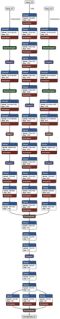 |
Fig. A.1 PICZL architecture, showcasing its three-threaded design. Two threads are dedicated to processing image inputs, while the third handles numerical data. The model’s output layer generates distinct vectors corresponding to the means, standard deviations, and weights of multiple Gaussian distributions. This design enables the production of full PDFs, allowing the network to capture uncertainties. Question marks as the first dimension per thread input correspond to the (variable) sample size. |
Appendix B LS10 seeing for different samples
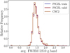 |
Fig. B.1 Histograms of the weighted average FWHM (seeing) values for the PICZL training, validation, and CSC2 blind samples. The close alignment of these distributions indicates no significant mismatch between the datasets, as they represent all-sky sampling. This similarity supports the applicability of the training sample to blind samples of comparable seeing. |
Appendix C CSC2 blind sample results
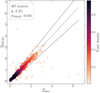 |
Fig. C.1 Scatter plot of the CSC2 sample color-coded by point density, illustrating the performance of PICZL on previously unseen data, as the majority of sources lie within the defined outlier boundary, demonstrating the prediction robustness. Sources identified as outliers generally scatter close to the boundary, with only a few instances of significant deviations or catastrophic failures. |
Appendix D Photometric errors in LS10
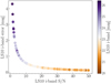 |
Fig. D.1 Relationship between S/N and the associated photometric error for the LS10 i-band, considering all sources from Table 1. Each point is color-coded according to the i-band magnitude. A noticeable turning point is observed for sources with S/N ≲ 15, indicating a significant increase in magnitude error for sources fainter than ~ 22 magnitude. |
Appendix E XMM-SERVS sources in LS10
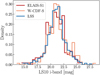 |
Fig. E.1 Histograms of LS10 i-band magnitudes for the three XMM-SERVS subsamples: ELAIS-S1, W-CDF-S, and LSS. The magnitudes are displayed as normalized densities to allow for direct comparison across the fields. These distributions extend to fainter magnitudes than those shown in Figure 15, accounting for the increased ηP denoted in Table 4. As the depth reached in PICZL’s LS10 training set is limited toward brighter magnitudes, a direct comparison between subsamples is only valid when conducted within a controlled parameter space, as shown in Figure 13. |
Appendix F Column description of released photo-z catalog
XID: Unique source ID assigned to each X-ray source in the original papers (see Chen et al. 2018; Ni et al. 2021)
SURVEY: Original survey where the source was detected
LS10_FULLID: Unique LS source ID assigned to optical counterpart. It is created by concatenating the LS coloumns RELEASE, BRICKID and OBJID.
CTP_LS10_RA: Right Ascension in degrees of the LS10 optical counterpart
CTP_LS 10_DEC: Declination in degrees of the LS 10 optical counterpart
SPECZ: spec-z from original catalog
PHZ_PICZL: Photo-z from PICZL
PHZ_PICZL_168: PICZL photo-z min at 1 sigma
PHZ_PICZL_u68: PICZL photo-z max at 1 sigma
PHZ_PICZL_199: PICZL photo-z min at 3 sigma
PHZ_PICZL_u99: PICZL photo-z max at 3 sigma
Appendix G PICZL run time
The computational demands for training and deploying PICZL depend mostly on the hardware configuration and dataset size. For our experiments, we leveraged a set of two Tesla V 100-PCIE graphics processing units (GPUs) each equipped with 32 GB of ready access memory (RAM), accompanied by a 48 core multi-thread CPU to accelerate the computational workload. This parallel processing capability significantly expedited the model training process, compared to running solely on a central CPU, allowing for faster convergence. Training a single model (refer to Figure A.1) on a dataset of 32 391 sources, corresponding to the 80:20 train-test split (refer to Table 1), each with 108 features (56 of which are images), takes approximately 25 minutes for 600 epochs. The use of an ensemble further scales the processing time by the number of models trained, with ensemble optimization depending on user preferences, making it difficult to provide a fixed time estimate. After finalizing the model, computing photo-z for 1393 sources in the XMM-SERVS W-CDF-S field, as displayed via Table 4, takes roughly 17 seconds. The storage requirements for the data used in this sample corresponds to approximately 250 MB (refer to Table 2). Looking ahead, upcoming surveys such as Euclid and LSST will produce higher-resolution images, demanding increased storage and computational resources due to larger data volumes and pixel counts. If the input dimensions were to increase, for instance, from 23x23 pixels to 64x64 pixels, the computational burden would rise significantly. While our current architecture of 32 GB RAM per GPU is efficient for the current input sizes, processing larger cutouts may necessitate either more GPUs or GPUs with higher memory capacity to maintain feasible training times and performance. In scenarios where larger input sizes are anticipated, a thoughtful approach to model architecture and resource allocation will be crucial. Therefore, adapting to the capabilities of the hardware will be key to successfully utilizing the methods in the context of future data from LSST and Euclid, particularly given the much larger sample sizes that we expect from these surveys. Finally, performance will also improve by having PICZL revised by an expert software developer.
References
- Abdalla, F. B., Banerji, M., Lahav, O., & Rashkov, V. 2011, MNRAS, 417, 1891 [NASA ADS] [CrossRef] [Google Scholar]
- Aird, J., Nandra, K., Laird, E. S., et al. 2010, MNRAS, 401, 2531 [Google Scholar]
- Ait-Ouahmed, R., Arnouts, S., Pasquet, J., Treyer, M., & Bertin, E. 2023, A&A, 683, A26 [Google Scholar]
- Akiba, T., Sano, S., Yanase, T., Ohta, T., & Koyama, M. 2019, arXiv e-prints [arXiv: 1907.10902] [Google Scholar]
- Alexander, D. M., Davis, T. M., Chaussidon, E., et al. 2023, ApJ, 165, 124 [CrossRef] [Google Scholar]
- Almeida, A., Anderson, S. F., Argudo-Fernández, M., et al. 2023, ApJS, 267, 44 [NASA ADS] [CrossRef] [Google Scholar]
- Almosallam, I. A., Jarvis, M. J., & Roberts, S. J. 2016, MNRAS, 462, 726 [Google Scholar]
- Ananna, T. T., Salvato, M., LaMassa, S., et al. 2017, ApJ, 850, 66 [Google Scholar]
- Arnouts, S., & Ilbert, O. 2011, Astrophysics Source Code Library [record ascl:1108.009] [Google Scholar]
- Autenrieth, M., van Dyk, D. A., Trotta, R., & Stenning, D. C. 2023, ASA Data Sci. J., 17, 1 [Google Scholar]
- Baum, W. 1957, ApJ, 62, 6 [CrossRef] [Google Scholar]
- Beck, R., Dobos, L., Budavári, T., Szalay, A., & Csabai, I. 2017, Astron. Comput., 19, 34 [NASA ADS] [CrossRef] [Google Scholar]
- Bell, E. F., Wolf, C., Meisenheimer, K., et al. 2004, ApJ, 608, 752 [NASA ADS] [CrossRef] [Google Scholar]
- Benitez, N. 2000, ApJ, 536, 571 [CrossRef] [Google Scholar]
- Bertin, E., & Arnouts, S. 1996, A&AS, 117, 393 [NASA ADS] [CrossRef] [EDP Sciences] [Google Scholar]
- Bettoni, D., Falomo, R., Kotilainen, J. K., Karhunen, K., & Uslenghi, M. 2015, MNRAS, 454, 4103 [NASA ADS] [CrossRef] [Google Scholar]
- Blanton, M. R., Bershady, M. A., Abolfathi, B., et al. 2017, ApJ, 154, 28 [Google Scholar]
- Boller, T., Freyberg, M. J., Trümper, J., et al. 2016, A&A, 588, A103 [NASA ADS] [CrossRef] [EDP Sciences] [Google Scholar]
- Bolton, A. S., Schlegel, D. J., Aubourg, E., et al. 2012, ApJ, 144, 144 [CrossRef] [Google Scholar]
- Bolzonella, M., Miralles, J.-M., & Pello’, R. 2000, A&A, 363, 476 [NASA ADS] [Google Scholar]
- Bordoloi, R., Lilly, S. J., & Amara, A. 2010, MNRAS, 406, 881 [NASA ADS] [Google Scholar]
- Boutsia, K., Grazian, A., Calderone, G., et al. 2020, ApJS, 250, 26 [NASA ADS] [CrossRef] [Google Scholar]
- Brammer, G. B., van Dokkum, P. G., & Coppi, P. 2008, ApJ, 686, 1503 [Google Scholar]
- Brandt, W. N., Ni, Q., Yang, G., et al. 2018, arXiv e-prints [arXiv: 1811.06542] [Google Scholar]
- Breiman, L. 2001, Mach. Learn., 545, 5 [NASA ADS] [CrossRef] [Google Scholar]
- Brescia, M., Cavuoti, S., Longo, G., & Stefano, V. D. 2014, A&A, 568, A126 [NASA ADS] [CrossRef] [EDP Sciences] [Google Scholar]
- Brescia, M., Salvato, M., Cavuoti, S., et al. 2019, MNRAS, 489, 663 [NASA ADS] [CrossRef] [Google Scholar]
- Brunner, H., Liu, T., Lamer, G., et al. 2022, A&A, 661, A1 [NASA ADS] [CrossRef] [EDP Sciences] [Google Scholar]
- Buchner, J., Georgakakis, A., Nandra, K., et al. 2015, ApJ, 802, 89 [Google Scholar]
- Campagne, J.-E. 2020, arXiv e-prints [arXiv:2002.10154] [Google Scholar]
- Cardamone, C. N., van Dokkum, P. G., Urry, C. M., et al. 2010, ApJS, 189, 270 [Google Scholar]
- Carliles, S., Budavári, T., Heinis, S., Priebe, C., & Szalay, A. S. 2010, ApJ, 712, 511 [NASA ADS] [CrossRef] [Google Scholar]
- Cavuoti, S., Amaro, V., Brescia, M., et al. 2016, MNRAS, 465, 1959 [Google Scholar]
- Chen, C.-T. J., Brandt, W. N., Luo, B., et al. 2018, MNRAS, 478, 2132 [NASA ADS] [CrossRef] [Google Scholar]
- Cirasuolo, M., Fairley, A., Rees, P., et al. 2020, The Messenger 180, 10 [NASA ADS] [Google Scholar]
- Coffey, D., Salvato, M., Merloni, A., et al. 2019, A&A, 625, A123 [NASA ADS] [CrossRef] [EDP Sciences] [Google Scholar]
- Cohen, T., & Welling, M. 2016, in Proceedings of The 33rd International Conference on Machine Learning, eds. M. F. Balcan, & K. Q. Weinberger (New York, USA: PMLR), 48, 2990 [Google Scholar]
- Collister, A. A., & Lahav, O. 2004, PASP, 116, 345 [NASA ADS] [CrossRef] [Google Scholar]
- Comparat, J., Merloni, A., Dwelly, T., et al. 2020, A&A, 636, A97 [NASA ADS] [CrossRef] [EDP Sciences] [Google Scholar]
- Connolly, A. J., Csabai, I., Szalay, A. S., et al. 1995, ApJ, 110, 2655 [Google Scholar]
- Croom, S. M., Smith, R. J., Boyle, B. J., et al. 2004, MNRAS, 349, 1397 [NASA ADS] [CrossRef] [Google Scholar]
- Dahlen, T., Mobasher, B., Faber, S. M., et al. 2013, ApJ, 775, 93 [Google Scholar]
- Dark Energy Survey Collaboration (Abbott, T., et al.) 2016, MNRAS, 460, 1270 [Google Scholar]
- Dawid, A. P. 1984, J. R. Stat. Soc. Ser. A, 147, 278 [Google Scholar]
- De Jong, R. S., Agertz, O., Berbel, A. A., et al. 2019, The Messenger, 175, 3 [NASA ADS] [Google Scholar]
- Deru, M., & Ndiaye, A. 2019, Deep Learning mit TensorFlow, Keras und TensorFlow.js (Germany: Rheinwerk Verlag) [Google Scholar]
- DESI-Collaboration (Aghamousa, A., et al.) 2016, arXiv e-prints [arXiv: 1611.00036] [Google Scholar]
- Desprez, G., Paltani, S., Coupon, J., et al. 2020, A&A, 644, A31 [NASA ADS] [CrossRef] [EDP Sciences] [Google Scholar]
- Dey, A., Schlegel, D. J., Lang, D., et al. 2019, ApJ, 157, 168 [CrossRef] [Google Scholar]
- Dey, B., Andrews, B. H., Newman, J. A., et al. 2022a, MNRAS, 515, 5285 [NASA ADS] [CrossRef] [Google Scholar]
- Dey, B., Newman, J. A., Andrews, B. H., et al. 2022b, arXiv e-prints [arXiv: 2110.15209] [Google Scholar]
- D’Isanto, A., & Polsterer, K. L. 2018, A&A, 609, A111 [Google Scholar]
- Donoso-Oliva, C., Becker, I., Protopapas, P., et al. 2023, A&A, 670, A54 [NASA ADS] [CrossRef] [EDP Sciences] [Google Scholar]
- Drlica-Wagner, A., Carlin, J. L., Nidever, D. L., Ferguson, P. S., & Kuropatkin, N. 2021, ApJS, 256, 2 [NASA ADS] [CrossRef] [Google Scholar]
- Duda, R. O., Hart, P. E., & Stork, D. G. 1973, Pattern Classification, 2nd edn. (New York: Wiley) [Google Scholar]
- Duncan, K. J. 2022, MNRAS, 512, 3662 [NASA ADS] [CrossRef] [Google Scholar]
- Dwelly, T., Salvato, M., Merloni, A., et al. 2017, MNRAS, 469, 1065 [Google Scholar]
- Eriksen, M., Alarcon, A., Cabayol, L., et al. 2020, MNRAS, 497, 4565 [CrossRef] [Google Scholar]
- Euclid Collaboration (Mellier, Y., et al.) 2024, A&A, in press, https://doi.org/10.1051/0004-6361/202450810 [Google Scholar]
- Fan, X., Banados, E., & Simcoe, R. A. 2022, ARA&A, 61, 373 [Google Scholar]
- Ferrarese, L., & Merritt, D. 2000, ApJ, 539, L9 [Google Scholar]
- Flaugher, B., Diehl, H. T., Honscheid, K., et al. 2015, ApJ, 150, 150 [Google Scholar]
- Fotopoulou, S., & Paltani, S. 2018, A&A, 619, A14 [NASA ADS] [CrossRef] [EDP Sciences] [Google Scholar]
- Fukushima, K. 1980, Biol. Cybernet., 36, 193 [CrossRef] [Google Scholar]
- Gebhardt, K., Bender, R., Bower, G., et al. 2000, ApJ, 539, L13 [Google Scholar]
- Georgakakis, A., Aird, J., Buchner, J., et al. 2015, MNRAS, 453, 1946 [Google Scholar]
- Géron, A. 2019, Hands-On Machine Learning with Scikit-Learn, Keras & TensorFlow (Sebastopol, California: O’Reilly, Kiwisoft S.A.S.) [Google Scholar]
- Gneiting, T., Raftery, A., Westveld, A., & Goldman, A. 2005, Mon. Weather Rev., 133, 1098 [Google Scholar]
- Gomes, Z., Jarvis, M. J., Almosallam, I. A., & Roberts, S. J. 2017, MNRAS, 475, 331 [Google Scholar]
- Grimit, E., Gneiting, T., Berrocal, V., & Johnson, N. 2006, Quarter. J. R. Meteorol. Soc., 132, 2925 [Google Scholar]
- Goodfellow, I., Bengio, Y., & Courville, A. 2016, Deep Learning (Massachusetts: Massachusetts Institute of Technology) [Google Scholar]
- Hatfield, P. W., Almosallam, I. A., Jarvis, M. J., et al. 2020, MNRAS, 498, 5498 [NASA ADS] [CrossRef] [Google Scholar]
- Hayat, M. A., Stein, G., Harrington, P., Lukic , Z., & Mustafa, M. 2021, ApJ, 911, L33 [NASA ADS] [CrossRef] [Google Scholar]
- He, K., Zhang, X., Ren, S., & Sun, J. 2015, Deep Residual Learning for Image Recognition (USA: IEEE) [Google Scholar]
- Heckman, T. M., & Best, P. N. 2014, ARA&A, 52, 589 [Google Scholar]
- Henghes, B., Thiyagalingam, J., Pettitt, C., Hey, T., & Lahav, O. 2022, MNRAS, 512, 1696 [NASA ADS] [CrossRef] [Google Scholar]
- Hewett, P. C., & Wild, V. 2010, MNRAS, 405, 2302 [NASA ADS] [Google Scholar]
- Hoyle, B. 2016, Astron. Comput., 16, 34 [NASA ADS] [CrossRef] [Google Scholar]
- Hsu, L.-T., Salvato, M., Nandra, K., et al. 2014, ApJ, 796, 60 [Google Scholar]
- Ilbert, O., Arnouts, S., McCracken, H. J., et al. 2006, A&A, 457, 841 [NASA ADS] [CrossRef] [EDP Sciences] [Google Scholar]
- Illingworth, G. D. 1999, Astrophysics, 269, 165 [NASA ADS] [Google Scholar]
- Ivezic, Z., Kahn, S. M., Tyson, J. A., et al. 2019, ApJ, 873, 111 [NASA ADS] [CrossRef] [Google Scholar]
- Jones, D. M., & Heavens, A. F. 2018, MNRAS, 483, 2487 [Google Scholar]
- Jones, E., & Singal, J. 2017, A&A, 600, A113 [NASA ADS] [CrossRef] [EDP Sciences] [Google Scholar]
- Kind, M. C., & Brunner, R. J. 2013, MNRAS, 432, 1483 [NASA ADS] [CrossRef] [Google Scholar]
- Kingma, D. P., & Ba, J. 2017, Adam: A Method for Stochastic Optimization (The Netherlands: University of Amsterdam) [Google Scholar]
- Kluge, M., Comparat, J., Liu, A., et al. 2024, A&A, 688, A210 [NASA ADS] [CrossRef] [EDP Sciences] [Google Scholar]
- Kollmeier, J., Anderson, S. F., Blanc, G. A., et al. 2019, BAAS, 51, 274 [NASA ADS] [Google Scholar]
- Kormendy, J., & Ho, L. C. 2013, ARA&A, 51, 511 [Google Scholar]
- Kullback, S., & Leibler, R. A. 1951, Ann. Math. Stat., 22, 79 [CrossRef] [Google Scholar]
- LaMassa, S. M., Georgakakis, A., Vivek, M., et al. 2019, ApJ, 876, 50 [NASA ADS] [CrossRef] [Google Scholar]
- Lang, D. 2014, ApJ, 147, 108 [CrossRef] [Google Scholar]
- Lang, D., Hogg, D. W., & Mykytyn, D. 2016, Astrophysics Source Code Library [record ascl:1604.008] [Google Scholar]
- Laurino, O., D’Abrusco, R., Longo, G., & Riccio, G. 2011, MNRAS, 418, 2165 [NASA ADS] [CrossRef] [Google Scholar]
- LeCun, Y., Boser, B., Denker, J. S., et al. 1989, Neural Comput., 1, 541 [NASA ADS] [CrossRef] [Google Scholar]
- Lecun, Y., Bottou, L., Bengio, Y., & Haffner, P. 1998, Proc. IEEE, 86, 2278 [Google Scholar]
- Li, C., Zhang, Y., Cui, C., et al. 2021, MNRAS, 509, 2289 [CrossRef] [Google Scholar]
- Li, C., Zhang, Y., Cui, C., et al. 2022, MNRAS, 518, 513 [CrossRef] [Google Scholar]
- Lin, Q., Fouchez, D., Pasquet, J., et al. 2022, A&A, 662, A36 [NASA ADS] [CrossRef] [EDP Sciences] [Google Scholar]
- Lines, N. E. P., Roset, J. F.-Q., & Scaife, A. M. M. 2024, RAS Tech. Instrum., 3, 347 [Google Scholar]
- Liu, Z., Mao, H., Wu, C.-Y., et al. 2022, in Proceedings of the IEEE/CVF Conference on Computer Vision and Pattern Recognition (CVPR), 11976 [Google Scholar]
- Luken, K. J., Norris, R. P., & Park, L. A. F. 2019, PASP, 131, 108003 [NASA ADS] [CrossRef] [Google Scholar]
- Luo, B., Brandt, W. N., Xue, Y. Q., et al. 2010, ApJS, 187, 560 [NASA ADS] [CrossRef] [Google Scholar]
- Lyke, B. W., Higley, A. N., McLane, J. N., et al. 2020, ApJS, 250, 8 [NASA ADS] [CrossRef] [Google Scholar]
- Ma, L., Lu, Z., Shang, L., & Li, H. 2015, arXiv e-prints [arXiv:1504.06063] [Google Scholar]
- Madau, P., & Dickinson, M. 2014, ARA&A, 52, 415 [Google Scholar]
- Mainzer, A., Bauer, J., Grav, T., et al. 2011, ApJ, 731, 53 [Google Scholar]
- Malz, A. I., Marshall, P. J., DeRose, J., et al. 2018, ApJ, 156, 35 [CrossRef] [Google Scholar]
- Masters, D., Capak, P., Stern, D., et al. 2015, ApJ, 813, 53 [Google Scholar]
- Masters, D. C., Stern, D. K., Cohen, J. G., et al. 2019, ApJ, 877, 81 [Google Scholar]
- Mauduit, J.-C., Lacy, M., Farrah, D., et al. 2012, PASP, 124, 714 [Google Scholar]
- Meisner, A. M., Lang, D., & Schlegel, D. J. 2017, ApJ, 153, 38 [CrossRef] [Google Scholar]
- Melchior, P., Moolekamp, F., Jerdee, M., et al. 2018, Astron. Comput., 24, 129 [Google Scholar]
- Merloni, A., Predehl, P., Becker, W., et al. 2012, arXiv e-prints [arXiv:1209.3114] [Google Scholar]
- Merloni, A., Lamer, G., Liu, T., et al. 2024, A&A, 682, A34 [NASA ADS] [CrossRef] [EDP Sciences] [Google Scholar]
- Meshcheryakov, A., Glazkova, V., Gerasimov, S., & Mashechkin, I. 2018, Astron. Lett., 44, 735 [NASA ADS] [CrossRef] [Google Scholar]
- Mountrichas, G., Corral, A., Masoura, V. A., et al. 2017, A&A, 608, A39 [NASA ADS] [CrossRef] [EDP Sciences] [Google Scholar]
- Newman, J. A., & Gruen, D. 2022, ARA&A, 60, 363 [NASA ADS] [CrossRef] [Google Scholar]
- Ni, Q., Brandt, W. N., Chen, C.-T., et al. 2021, ApJS, 256, 21 [CrossRef] [Google Scholar]
- Nishizawa, A. J., Hsieh, B.-C., Tanaka, M., & Takata, T. 2020, PASJ, 70, S9 [Google Scholar]
- Norris, R. P., Salvato, M., Longo, G., et al. 2019, PASP, 131, 108004 [Google Scholar]
- O’Shea, K., & Nash, R. 2015, arXiv e-prints [arXiv: 1511.08458] [Google Scholar]
- Padovani, P., Alexander, D. M., Assef, R. J., et al. 2017, A&ARv, 25, 1 [NASA ADS] [CrossRef] [Google Scholar]
- Parker, L., Lanusse, F., Golkar, S., et al. 2024, MNRAS, 531, 4990 [Google Scholar]
- Pasquet, J., Bertin, E., Treyer, M., Arnouts, S., & Fouchez, D. 2018, A&A, 621, A26 [Google Scholar]
- Pierce, C. M., Lotz, J. M., Primack, J. R., et al. 2010, MNRAS, 408, 139 [Google Scholar]
- Povic, M., Sánchez-Portal, M., Garcia, A. M. P., et al. 2012, A&A, 541, A118 [NASA ADS] [CrossRef] [EDP Sciences] [Google Scholar]
- Predehl, P., Andritschke, R., Arefiev, V., et al. 2021, A&A, 647, A1 [EDP Sciences] [Google Scholar]
- Rau, M. M., Seitz, S., Brimioulle, F., et al. 2015, MNRAS, 452, 3710 [NASA ADS] [CrossRef] [Google Scholar]
- Revsbech, E. A., Trotta, R., & van Dyk, D. A. 2017, MNRAS, 473, 3969 [Google Scholar]
- Rosenbaum, P., & Rubin, D. 1984, J. Am. Stat. Assoc., 79, 516 [CrossRef] [Google Scholar]
- Rosenblatt, F. 1958, Psychol. Rev. 65, 6 [Google Scholar]
- Ruiz, A., Corral, A., Mountrichas, G., & Georgantopoulos, I. 2018, A&A, 618, A52 [NASA ADS] [CrossRef] [EDP Sciences] [Google Scholar]
- Sadeh, I., Abdalla, F. B., & Lahav, O. 2016, PASP, 128, 104502 [NASA ADS] [CrossRef] [Google Scholar]
- Salvato, M., Hasinger, G., Ilbert, O., et al. 2008, ApJ, 690, 1250 [Google Scholar]
- Salvato, M., Ilbert, O., Hasinger, G., et al. 2011, ApJ, 742, 61 [Google Scholar]
- Salvato, M., Ilbert, O., & Hoyle, B. 2018, Nat. Astron., 3, 212 [CrossRef] [Google Scholar]
- Salvato, M., Wolf, J., Dwelly, T., et al. 2022, A&A, 661, A3 [NASA ADS] [CrossRef] [EDP Sciences] [Google Scholar]
- Sánchez, C., Kind, M. C., Lin, H., et al. 2014, MNRAS, 445, 1482 [Google Scholar]
- Sanchez, J., Mendoza, I., Kirkby, D. P., & Burchat, P. R. 2021, J. Cosmol. Astropart. Phys., 2021, 043 [Google Scholar]
- Savic, D. V., Jankov, I., Yu, W., et al. 2023, ApJ, 953, 138 [CrossRef] [Google Scholar]
- Saxena, A., Salvato, M., Roster, W., et al. 2024, A&A, 690, A365 [NASA ADS] [CrossRef] [EDP Sciences] [Google Scholar]
- Scaramella, R., Amiaux, J., Mellier, Y., et al. 2022, A&A, 662, A112 [NASA ADS] [CrossRef] [EDP Sciences] [Google Scholar]
- Schmidt, S. J., Malz, A. I., Soo, J. Y. H., et al. 2020, MNRAS, 499, 1587 [Google Scholar]
- Schuldt, S., Suyu, S. H., Cañ ameras, R., et al. 2021, A&A, 651, A55 [NASA ADS] [CrossRef] [EDP Sciences] [Google Scholar]
- Scolnic, D. M., Lochner, M., Gris, P., et al. 2018, arXiv e-prints [arXiv:1812.008516] [Google Scholar]
- Silva, D. R., Blum, R. D., Allen, L., et al. 2016, AAS Meeting Abstracts, 228, 317.02 [NASA ADS] [Google Scholar]
- Simm, T., Saglia, R., Salvato, M., et al. 2015, A&A, 584, A106 [NASA ADS] [CrossRef] [EDP Sciences] [Google Scholar]
- Soo, J. Y. H., Moraes, B., Joachimi, B., et al. 2017, MNRAS, 475, 3613 [Google Scholar]
- Stabenau, H. F., Connolly, A., & Jain, B. 2008, MNRAS, 387, 1215 [NASA ADS] [CrossRef] [Google Scholar]
- Steidel, C. C., Giavalisco, M., Dickinson, M., & Adelberger, K. L. 1996, ApJ, 112, 352 [Google Scholar]
- Tamura, N., Takato, N., Shimono, A., et al. 2016, SPIE, 9908, 990801 [Google Scholar]
- Treyer, M., MNRAS, 527, 651 [Google Scholar]
- Véron-Cetty, M. P., & Véron, P. 2010, A&A, 518, A10 [Google Scholar]
- Viroli, C., & McLachlan, G. J. 2017, Deep Gaussian Mixture Models (Berlin: Springer) [Google Scholar]
- Voges, W., Aschenbach, B., Boller, T., et al. 1999, arXiv e-prints [arXiv:astro-ph/9909315] [Google Scholar]
- Webb, N. A., Coriat, M., Traulsen, I., et al. 2020, A&A, 641, A136 [NASA ADS] [CrossRef] [EDP Sciences] [Google Scholar]
- Weiler, M., & Cesa, G. 2021, arXiv e-prints [arXiv: 1911.08251] [Google Scholar]
- Wilson, D., Nayyeri, H., Cooray, A., & Häußler, B. 2020, ApJ, 888, 83 [NASA ADS] [CrossRef] [Google Scholar]
- Wright, E. L., Eisenhardt, P. R. M., Mainzer, A. K., et al. 2010, ApJ, 140, 1868 [Google Scholar]
- Wu, Q., & Shen, Y. 2022, ApJS, 263, 42 [NASA ADS] [CrossRef] [Google Scholar]
- Wuyts, S., Förster Schreiber, N. M., van der Wel, A., et al. 2011, ApJ, 742, 96 [NASA ADS] [CrossRef] [Google Scholar]
- Yang, J., Fan, X., Gupta, A., et al. 2023, ApJS, 269, 27 [NASA ADS] [CrossRef] [Google Scholar]
- York, D. G., Adelman, J., John E. Anderson, J., et al. 2000, ApJ, 120, 1579 [CrossRef] [Google Scholar]
- Zhang, Y., & Zhao, Y. 2015, Data Sci. J., 14, 11 [NASA ADS] [CrossRef] [Google Scholar]
- Zhang, Y., Ma, H., Peng, N., Zhao, Y., & bing Wu, X. 2013, ApJ, 146, 22 [NASA ADS] [CrossRef] [Google Scholar]
- Zhao, D., Dalmasso, N., Izbicki, R., & Lee, A. B. 2021, PMLR, 161, 1830 [Google Scholar]
- Zhou, R., Newman, J. A., Mao, Y.-Y., et al. 2021, MNRAS, 501, 3309 [NASA ADS] [CrossRef] [Google Scholar]
- Zhou, R., Ferraro, S., White, M., et al. 2023, J. Cosmology Astropart. Phys., 2023, 097 [Google Scholar]
- Zou, H., Zhang, T., Zhou, Z., et al. 2017, ApJ, 153, 276 [Google Scholar]
Used interchangeably in both singular and plural cases.
Transforming probabilities into their logarithms simplifies the mathematical operations involved (multiplication into addition), rendering the function more amenable to optimization techniques such as gradient descent, facilitating the search for optimal model parameters.
All Tables
Overview of the relative fractions of source catalogs used in compiling our AGN training sample.
Overview of the various feature formats and dimensions utilized in PICZL’s multi-channel approach.
Comparison of bias, fraction of outliers, and variance between photo-z computed with PICZL for various subsamples.
All Figures
|
Fig. 1 Flowchart depicting the training sample down-selection pipeline. This includes the sample preprocessing (grey box) and the sample refinement, including redshift extension and duplicate removal below the dashed red line. |
| In the text | |
|
Fig. 2 Binned redshift histogram (top panel) and cumulative distribution (bottom panel) of the sources utilized in the PICZL AGN sample. Note that these samples are not necessarily rank ordered by importance but for improved readability. |
| In the text | |
|
Fig. 3 Grid of subplots showing various model inputs for PICZL. In the upper row: the LS10 ɡ-band image (a), along with its 2-D model flux (b), residual (c), and aperture flux map (d). In the bottom row: the original g-r color is shown in (a). The presence of a saturated pixel in the top right corner is visible, indicating the need for pre-processing. The result of the preprocessing is shown in b. The bottom panels c and d show the ɡ/r-band and w1/w2-band aperture flux maps, respectively. |
| In the text | |
|
Fig. 4 Angular size of sources with a fixed physical size of 20–40 kpc, as a function of redshift. The orange dashed line depicts a fixed image dimension of 23 pixels, assuming the LS10 spatial resolution of 0.262 arc seconds per pixel, which suffices to cover objects of 30 kpc diameters in size out to redshifts of ~ 0.3 ≤ ɀ ≤ 7.8. |
| In the text | |
|
Fig. 5 Example AGN in our sample, as seen by LS10, in the optical RGB image (left) and in the W1 image from NEOWISE7 (right). The spatial resolution is 0.262 arcseconds and 2.75 arcseconds per pixel, respectively. The size of the cutouts is 27.5 arc seconds × 27.5 arc seconds. |
| In the text | |
|
Fig. 6 Training (dashed) and Validation (solid) loss curves for a single PICZL model. The solid or dashed lines represent the mean loss values computed over a window size of 20, while the shaded areas denote the 1σ error range around the mean. The NLL loss is depicted in blue, while the normalized CRPS loss is shown in red. |
| In the text | |
|
Fig. 7 Binned scatter plots of photo-z obtained from our model ZPICZL versus spectroscopic redshift Zspec , for sources classified as type point-like (PSF, left) and extended (EXT, right). Each plot includes identity and two lines denoting the outlier boundary of |
| In the text | |
|
Fig. 8 Histogram distribution of the normalised residuals, overlaid with a Gaussian fit (orange). The parameters of the Gaussian distribution are determined by the prediction bias and σNMAD values obtained from Table 5 for the validation sample. |
| In the text | |
|
Fig. 9 Display of the QQ plot, comparing identity (flat histogram) against the PIT values derived from our redshift PDFs of the validation sample (top panel), and the differences between the QQ plot and identity, highlighting systematic biases or trends for the two morphological classes (PSF and EXT), shown in the bottom panel. For all panels, blue refers to results achieved with a single model (see Figure A.1) while orange reflects the results obtained when utilizing ensemble results (refer to Sect. 5.6). |
| In the text | |
|
Fig. 10 PICZL point estimates as a function of PDF width, represented by the difference between upper and lower 1σ values. Each data point is color-coded according to its r-band magnitude from the LS10. The tilt of the distribution traces the increased uncertainties for PDFs of fainter sources. Horizontal distributions represent areas of large uncertainty in the photo-z, indicating that PICZL errors are realistic. |
| In the text | |
|
Fig. 11 Examples of an inlier (orange) and an outlier (purple) PDF (left panel). By definition, the point estimate derived for the two sources from the main mode falls within or outside the grey shaded region. Both sources show a secondary peak in the PDF. We can define the probability of being an inlier (colored area under the PDF which coincides with the grey shaded area). Normalized |
| In the text | |
|
Fig. 12 Fraction of sources having a PDFs presenting secondary peaks for outliers (burgundy) and inliers (blue) are shown in the upper panel with corresponding recovery fraction for outliers (bottom panel). Both metrics are plotted as a function of the relative prominence threshold of the secondary peak. |
| In the text | |
|
Fig. 13 Outlier fraction (top row) as a function of LS10 i-band magnitude (left) and LS10 i-band S/N (right), comparing the original photo-z from XMM-SERVS to the photo-z computed with PICZL. The XMM-SERVS photo-z results are shown both with and without the inclusion of sources for which XMM-SERVS photo-z failed (photo-z = −99). The shaded regions represent the range of XMM-SERVS outlier fractions across the ELAIS-S1, W-CDF-S, and LSS fields. The bottom row panels depict the range of XMM-SERVS variance in the three fields as a function of LS10 i-band magnitude and S/N. PICZL demonstrates a lower outlier fraction for brighter sources while maintaining comparable accuracy to the original photo-z estimates. Additionally, PICZL successfully computes photo-z for sources that are failures in the original methods. |
| In the text | |
|
Fig. 14 Normalized residuals for PICZL photo-z compared to XMM-SERVS photo-z, using data from XMM-SERVS ELAIS-S1. PICZL outliers are shown as triangles, XMM-SERVS outliers as stars, and sources that are outliers in both methods are depicted as octagons. All sources are color-coded based on their LS10 i-band magnitude. |
| In the text | |
|
Fig. 15 Prediction bias (top row), fraction of outliers (second row), variance (third row), and number count (fourth row) as a function of magnitude (r-band from LS10), 0.2–2.3 keV X-ray flux, and spec-ɀ, categorized by type (extended (EXT)/point-like (PSF)). |
| In the text | |
|
Fig. 16 Cumulative fraction of outliers as function of absolute magnitudes, to validate their classification based on TYPE. The left panel shows outliers classified as PSF, where most sources have absolute magnitudes consistent with AGN or QSO characteristics. In the right panel, 16% of EXT-classified outliers exhibit absolute magnitudes more typical of QSOs. |
| In the text | |
|
Fig. A.1 PICZL architecture, showcasing its three-threaded design. Two threads are dedicated to processing image inputs, while the third handles numerical data. The model’s output layer generates distinct vectors corresponding to the means, standard deviations, and weights of multiple Gaussian distributions. This design enables the production of full PDFs, allowing the network to capture uncertainties. Question marks as the first dimension per thread input correspond to the (variable) sample size. |
| In the text | |
|
Fig. B.1 Histograms of the weighted average FWHM (seeing) values for the PICZL training, validation, and CSC2 blind samples. The close alignment of these distributions indicates no significant mismatch between the datasets, as they represent all-sky sampling. This similarity supports the applicability of the training sample to blind samples of comparable seeing. |
| In the text | |
|
Fig. C.1 Scatter plot of the CSC2 sample color-coded by point density, illustrating the performance of PICZL on previously unseen data, as the majority of sources lie within the defined outlier boundary, demonstrating the prediction robustness. Sources identified as outliers generally scatter close to the boundary, with only a few instances of significant deviations or catastrophic failures. |
| In the text | |
|
Fig. D.1 Relationship between S/N and the associated photometric error for the LS10 i-band, considering all sources from Table 1. Each point is color-coded according to the i-band magnitude. A noticeable turning point is observed for sources with S/N ≲ 15, indicating a significant increase in magnitude error for sources fainter than ~ 22 magnitude. |
| In the text | |
|
Fig. E.1 Histograms of LS10 i-band magnitudes for the three XMM-SERVS subsamples: ELAIS-S1, W-CDF-S, and LSS. The magnitudes are displayed as normalized densities to allow for direct comparison across the fields. These distributions extend to fainter magnitudes than those shown in Figure 15, accounting for the increased ηP denoted in Table 4. As the depth reached in PICZL’s LS10 training set is limited toward brighter magnitudes, a direct comparison between subsamples is only valid when conducted within a controlled parameter space, as shown in Figure 13. |
| In the text | |
Current usage metrics show cumulative count of Article Views (full-text article views including HTML views, PDF and ePub downloads, according to the available data) and Abstracts Views on Vision4Press platform.
Data correspond to usage on the plateform after 2015. The current usage metrics is available 48-96 hours after online publication and is updated daily on week days.
Initial download of the metrics may take a while.