| Issue |
A&A
Volume 690, October 2024
|
|
|---|---|---|
| Article Number | A365 | |
| Number of page(s) | 17 | |
| Section | Extragalactic astronomy | |
| DOI | https://doi.org/10.1051/0004-6361/202450886 | |
| Published online | 24 October 2024 | |
CIRCLEZ : Reliable photometric redshifts for active galactic nuclei computed solely using photometry from Legacy Survey Imaging for DESI
1
Max-Planck-Institut für extraterrestrische Physik, Giessenbachstr. 1, 85748 Garching, Germany
2
Technical University of Munich Department of Computer Science – I26, Boltzmannstr. 3, 85748 Garching b. München, Germany
3
Exzellenzcluster ORIGINS, Boltzmannstr. 2, D-85748 Garching, Germany
4
LMU Munich, Arnold Sommerfeld Center for Theoretical Physics, Theresienstr. 37, 80333 München, Germany
5
LMU Munich, Universität-Sternwarte, Scheinerstr. 1, 81679 München, Germany
6
Cerro Tololo Inter-American Observatory/NSF’s NOIRLab, Casilla 603, La Serena, Chile
7
Perimeter Institute for Theoretical Physics, 31 Caroline St. North, Waterloo, ON N2L 2Y5, Canada
8
Lawrence Berkeley National Laboratory, 1 Cyclotron Road, Berkeley, CA 94720, USA
9
National Optical Astronomy Observatory, 950 N. Cherry Avenue, Tucson, AZ 85719, USA
10
NSF National Optical/Infrared Research Laboratory, 950 N. Cherry Ave, Tucson, AZ 85719, USA
11
Department of Physics & Astronomy, University of Wyoming, 1000 E. University, Department 3905, Laramie, WY 8207, USA
12
Instituto de Estudios Astrofísicos, Facultad de Ingeniería y Ciencias, Universidad Diego Portales, Av. Ejército Libertador 441, Santiago, Chile
13
Instituto de Estudios Astrofísicos, Universidad Diego Portales, Av. Ejército Libertador 441, Santiago 8370191, Chile
14
Kavli Institute for Astronomy and Astrophysics, Peking University, Beijing 100871, China
15
Núcleo de Astronomía de la Facultad de Ingeniería, Universidad Diego Portales, Av. Ejército Libertador 441, Santiago 22, Chile
16
Space Telescope Science Institute, 3700 San Martin Drive, Baltimore MD 21218, USA
17
Department of Astronomy, University of Washington, Box 351580, Seattle, WA 98195, USA
18
Department of Astronomy, University of Illinois at Urbana-Champaign, Urbana, IL 61801, USA
19
National Center for Supercomputing Applications, University of Illinois at Urbana-Champaign, Urbana, IL 61801, USA
20
Center for Artificial Intelligence Innovation, University of Illinois at Urbana-Champaign, 1205 West Clark Street, Urbana, IL 61801, USA
⋆ Corresponding author; This email address is being protected from spambots. You need JavaScript enabled to view it.
Received:
27
May
2024
Accepted:
16
July
2024
Abstract
Context. Photometric redshifts for galaxies hosting an accreting supermassive black hole in their center, known as active galactic nuclei (AGNs), are notoriously challenging. At present, they are most optimally computed via spectral energy distribution (SED) fittings, assuming that deep photometry for many wavelengths is available. However, for AGNs detected from all-sky surveys, the photometry is limited and provided by a range of instruments and studies. This makes the task of homogenizing the data challenging, presenting a dramatic drawback for the millions of AGNs that wide surveys such as SRG/eROSITA are poised to detect.
Aims. This work aims to compute reliable photometric redshifts for X-ray-detected AGNs using only one dataset that covers a large area: the tenth data release of the Imaging Legacy Survey (LS10) for DESI. LS10 provides deep grizW1-W4 forced photometry within various apertures over the footprint of the eROSITA-DE survey, which avoids issues related to the cross-calibration of surveys.
Methods. We present the results from CIRCLEZ, a machine-learning algorithm based on a fully connected neural network. CIRCLEZ is built on a training sample of 14 000 X-ray-detected AGNs and utilizes multi-aperture photometry, mapping the light distribution of the sources.
Results. The accuracy (σNMAD) and the fraction of outliers (η) reached in a test sample of 2913 AGNs are equal to 0.067 and 11.6%, respectively. The results are comparable to (or even better than) what was previously obtained for the same field, but with much less effort in this instance. We further tested the stability of the results by computing the photometric redshifts for the sources detected in CSC2 and Chandra-COSMOS Legacy, reaching a comparable accuracy as in eFEDS when limiting the magnitude of the counterparts to the depth of LS10.
Conclusions. The method can be applied to fainter samples of AGNs using deeper optical data from future surveys (for example, LSST, Euclid), granting LS10-like information on the light distribution beyond the morphological type. Along with this paper, we have released an updated version of the photometric redshifts (including errors and probability distribution functions) for eROSITA/eFEDS.
Key words: methods: data analysis / methods: statistical / galaxies: active / galaxies: distances and redshifts
© The Authors 2024
 Open Access article, published by EDP Sciences, under the terms of the Creative Commons Attribution License (https://creativecommons.org/licenses/by/4.0), which permits unrestricted use, distribution, and reproduction in any medium, provided the original work is properly cited.
This article is published in open access under the Subscribe to Open model.
Open Access funding provided by Max Planck Society.
1. Introduction
It is now broadly accepted that in their lifetime, most (massive) galaxies will go through phase(s) when the supermassive black hole (SMBH) that they host is accreting at a significant fraction of its Eddington limit (for example, Madau & Dickinson 2014). While simulations show that feedback from these active galactic nuclei (AGNs) is necessary to regulate star formation in their host galaxies (for example, Di Matteo et al. 2005; Croton et al. 2006), in observational terms, the interplay between the host and the SMBH is still a matter of study. Further progress requires diverse samples of AGNs to be studied in detail, so accurate redshift estimates are necessary. While the number of multi-slit and multifiber spectrographs mounted on large telescopes is ever increasing (for example, SDSS: Kollmeier et al., in prep.; DESI: Levi et al. (2013); PFS: Takada et al. (2014); Moons: Cirasuolo et al. (2011); 4MOST: de Jong (2019)), thereby raising the completeness of the spectroscopic follow-up of AGNs, the urgent need to develop algorithms for the computation of reliable photometric redshifts (photo-z) for these types of objects remains. Deep photometric surveys like Euclid (Euclid Collaboration 2024) and LSST (Ivezić et al. 2019b) will provide huge samples of AGNs at a speed and depth that will not be matched by the new spectrographs. Photo-z for AGNs are challenging because the relative host or nucleus contribution to the emission is unknown a priori and even a modest contribution to the host galaxy SEDs by the continuum emission from the AGN hides the features used for identifying the redshift. The net result is a large fraction of sources having multiple possible redshifts (degeneracies).
Both machine learning techniques and SED fittings have been adopted (see Salvato et al. 2018a, for a review) in an attempt to improve on the results (for example, Table 1). What we have learned is: (a) a large number of photometric points is needed to break such degeneracies (for example, Brescia et al. 2019; b) photometry from narrow and intermediate bands is more valuable as opposed to mid-infrared (MIR) broadband photometry given their increased ability in pinpointing the emission lines and their intensity, thereby separating star-forming sources from AGN-powered objects. (Salvato et al. 2009; Cardamone et al. 2010; Luo et al. 2010; Hsu et al. 2014; c) machine learning can reach high accuracies for sources represented by the training sample at the cost of a very high fraction of outliers for sources outside the parameter space (for example, Duncan et al. 2018; Norris et al. 2019; Salvato et al. 2022; d) SED fitting performs well, granted that a redshift prior (for example, expressed via a redshift-dependent absolute magnitude range) is applied and the templates are appropriately selected (Luo et al. 2010; Fotopoulou et al. 2012; Hsu et al. 2014; Ananna et al. 2017; e) due to the presence of more features in the SED (for example, Lyman break, Balmer break), the quality of the photo-zs for inactive galaxies (computed either via SED fitting or via machine learning) remains superior to the photo-zs for AGNs; and (f) for AGN-dominated sources (more specifically, X-ray bright), obtaining reliable redshifts is more of a challenge (Brescia et al. 2019). All the works mentioned above relied on deep, PSF-homogenized photometry in many bands across the electromagnetic spectrum in pencil-beam areas, which is challenging to achieve for wide- or all-sky area surveys.
Accuracy and fraction of outliers obtained for X-ray surveys at different X-ray depths.
In fact, in the computation of photo-zs for the about 22 000 AGNs detected by eROSITA (Predehl et al. 2021; Merloni et al. 2024) in eFEDS Salvato et al. (2022) already pointed out how the inhomogeneity of the data quality drastically affects the reliability of the results1. Using the traditional method, for eRASS:8 in the best case scenario, we expect results that are not better than an accuracy of 0.07 and a fraction of outliers of 25%, after an extenuating effort of homogenization of the photometry from various surveys covering from UV to MIR. We consider whether this showcases significant issues for computing photo-zs for AGNs detected by the eROSITA all-sky surveys. Certainly, this would be the case if we tried to determine the redshift using the total fluxes emitted by the AGNs (and errors) as the only input, as is typically done according to the standard approach.
We mention earlier in this work that the extension of the sources in optical images provides a prior on the possible redshift solutions (Salvato et al. 2009). We can go beyond the differentiation between extended and point-like sources using machine learning. The feature analysis of all parameters available in the SDSS DR9 (Ahn et al. 2012) and SDSS DR7 (Abazajian et al. 2009) of spectroscopically confirmed AGNs and galaxies presented in (D’Isanto et al. 2018), indicates that the photo-zs quality could have been improved (for example: smaller bias, smaller root mean square error) for the photo-zs computed using fluxes and colors, by considering features such as Petrosian magnitudes2. In particular, what was found is that ratios between magnitudes computed assuming different models (point source, exponential, de Vaoucouler, or the combination of exponential and de Vaucouler) carry relevant information. Similarly, in Nishizawa et al. (2020), the computation of photo-zs for extragalactic sources detected in the HSC survey (Aihara et al. 2018) was carried out with machine learning relying solely on the optical photometry measured at 1.3 and 1.5 arcsec apertures, computed on the basis of a PSF, an exponential, and a de Vaucouler profile. The accuracy achieved by this approach (albeit limited to the parameter space covered by their training sample) was comparable to or even better than the results obtained via SED fitting after combining optical data with UV, NIR, and MIR data (see Salvato et al. 2022, for a direct comparison). Recent works have also reported on attempts to compute the photo-zs using the images directly (for example, Schuldt et al. 2021, Roster et al., in prep.). All these facts indicate a value when considering the morphology, size, and, in particular, the light distribution (for example, in the form of an azimuth profile) when computing the photo-zs. This is because all these quantities are, at least partially, redshift-dependent. In particular, unlike the single total “model” flux per each photometric band (which is what most photometric surveys provide), the fluxes within different apertures, and/or assuming different model profiles of light distribution (exponential, Sersic, Point-like, etc.) carry with them information on the host and nucleus relative contribution.
This is confirmed by the work presented in Zhou et al. (2021, 2023). Those authors obtained photo-zs values for DESI sources using the data release 9 of the Legacy Imaging Survey and considering the magnitudes, along with the colors g–r, r − z, z − W1, half-light radius, axial ratio (ratio between semi-minor and semi-major axes), and a model weight. While the accuracy was extremely good for galaxies (below 0.02 in accuracy and fraction of outliers below 10%, depending on the sample), the accuracy reached for AGNs and QSOs is poor, with an accuracy of 0.07 and up to 33% outliers (η3) and a low accuracy (σNMAD4) of 0.085.
The latest Legacy Survey imaging for DESI Data Release (LS10; Dey et al. 2019), available since January 2023, and a newly available large sample of spectroscopically confirmed AGNs (see Sect. 3) allowed us to test this hypothesis further. Here, we present the results from CIRCLEZ, a machine learning algorithm based on a fully connected neural network (FCCN) that reliably computes photo-zs for AGNs using only the data available from Legacy Survey without adding additional information from external surveys at different wavelengths. More so than in the algorithm (very similar to DNNZ; Nishizawa et al. 2020), the innovation here is the use of new features (colors within apertures and the quality of the fit to the azimuth profile assuming different galaxy profile models), which (just as with the total fluxes) are correlated with redshift themselves. The increase in useful features allows us to break the degeneracy in the redshift solution typical of photo-zs for AGNs computed with a limited number of photometric bands. We demonstrate this by recomputing the photo-zs of eROSITA/eFEDS and comparing the results previously obtained via SED fitting with LEPHARE (Arnouts et al. 1999; Ilbert et al. 2006; Salvato et al. 2009) and via machine learning with DNNZ (Salvato et al. 2022). In addition, we tested the quality of the photo-zs for AGNs selected in the Chandra Source Catalog Release 2 (CSC26) and Legacy Chandra-COSMOS (a deep pencil-beam survey) for those sources with secure spectroscopic redshift. We show that for AGNs with the counterparts of brightness typical of LS10, the photo-zs are reliable, suggesting that the method could also be adopted for fainter sources, granted that features and training samples are available. This is relevant for surveys such as Euclid (Euclid Collaboration 2024) and LSST (Ivezić et al. 2019b).
In Sect. 2 we present the ancillary data and the features that will be adopted, while in Sect. 3, we describe the training sample. Section 4 presents the architecture of the algorithm and can be skipped if only the results of the application are of interest. In Sect. 5, we recompute the photo-zs for the extragalactic sources detected by eROSITA (Predehl et al. 2021; Merloni et al. 2024) in the eFEDS field (Brunner et al. 2022; Salvato et al. 2022), so that a direct comparison with the results from DNNZ (from Nishizawa et al. 2020) and LePHARE (from Salvato22) can be made. Finally, in Sect. 6, the ability of CIRCLEZ in computing photo-zs for generic X-ray surveys is tested using the AGN detected in CSC2 and Chandra-COSMOS Legacy (Civano et al. 2012; Marchesi et al. 2016). The discussion is presented in Sect. 7, while the summary and a few considerations about the new photometric surveys available to the community and the future of photo-zs are given in the conclusion, in Sect. 8. Further analysis on the importance of the features used by CIRCLEZ for computing photo-zs is presented in Appendix A.
2. The photometric data: Going beyond total model fluxes
Typically, photometric observations are confined to survey-specific patches on-sky, each equipped with its unique configuration of broad and narrow band filters and varying transmission profiles. For samples of sources defined over areas of the sky larger than the typical photometric survey-specific patches, the inhomogeneity in observational setups can introduce inconsistencies when attempting to standardize surveys and establish a unified framework that enables seamless integration and comparison across different survey datasets. The already unstable photo-zs computed for AGNs suffer from this inhomogeneity more than the photo-zs computed for galaxies, so all-sky surveys of AGNs, such as the samples generated from the eROSITA catalogs, would not have a homogeneous quality.
Fortunately, the Legacy imaging Survey for DESI (Dey et al. 2019) data release 10 (LS10) provides registered, background-subtracted, and calibrated “all-sky” photometry, covering the eROSITA-DE footprint almost entirely. Despite the coverage being limited to the four optical bands (see Fig. 1) and WISE, it provides photometry that goes beyond the total flux measured assuming a galaxy profile; thus, the question is whether access to these features is sufficient to estimate reliable photo-zs for AGNs, without the need to combine the data with Galex in UV (Bianchi 2014) and VHS (McMahon et al. 2013) or UKIDSS (Lawrence et al. 2007) in NIR, thus simplifying the work dramatically. We refer to the “content” section of LS107 for comprehensive information on the survey data, processing details, and coverage. In the following sections, we explore the features considered for CIRCLEZ.
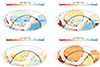 |
Fig. 1. Depth and coverage of LS10 in, clockwise, g, r, i, z filters. The black line delimits the eROSITA-DE area. The use of a common scale highlights the depth inhomogeneity of the data. For the rest of the paper, we use LS10-South (declination < 32.375deg), which is the area covered by the i band and also within the footprint of eROSITA. |
In this paper, we demonstrate that reliable photo-zs for AGNs with a limited number of photometric points are achievable by using (a) machine learning, (b) a training sample limited to AGNs and, more specifically, to X-ray detected AGNs, (c) considering parameters that correlate with redshift, in addition to standard parameters (magnitudes, colors, and morphology8). We identify the parameters as those that fully describe the light distribution of a source in its components (nuclear, bulge, disk) and are already available in the LS10 catalog. We describe the construction of the training sample in the next section, while here, we focus on describing the parameters (features) considered.
LS10 is composed of two distinct parts, LS10-North and LS10-South. LS10-North is obtained by combining two optical (g, r, z) surveys (Beijing-Arizona Sky Survey–BASS9; Mayall z-band Legacy Survey– MzLS10) in addition to the data obtained for DESI11 with the Dark Energy Camera (DECam) at the CTIO Blanco 4-m telescope. It corresponds to the northern portion of the Data Release 9 (Dey et al. 2019). LS10-South, compared to the Data Release 9, has deeper data taken with DECam in g, r, i, z. For the rest of the paper, we will refer to LS10-South as LS10, as the area covered by the i band (see Fig. 1), which almost completely maps the eROSITA-DE area. In particular, the data include all the observations taken within the DeROSITAs program (P.I. A. Zenteno; Zenteno et al., in prep). For each source detected in the four optical bands, LS1012 provides PSF-forced photometry (and related errors) in the optical g, r, i, z and MIR (W1, W2, W3, and W4) from all imaging through year 7 of NEOWISE-Reactivation, computed in multiple apertures (0.5, 0.75, 1.0, 1.5, 2.0, 3.5, 5.0, 7.0 arcsec radii in the optical and 3, 5, 7, 9, and 11 arcsec radii in the MIR). It also provides the total flux for each band, assuming the best model (indicated in the column TYPE: PSF”=stellar, “REX”=“round exponential galaxy”, “DEV”=deVauc, “EXP”=exponential, “SER”=Sersic profile) fitted to the azimuth profile in the r band, the quality of the fit for each model, together with an extensive catalog of observational attributes and flags indicating problematic observations.
Figure 2 provides a visual representation of the features used in our analysis and demonstrates the method’s strength. The figure shows the RGB image of a normal galaxy, a local AGN, and a QSO. In the Second row, the azimuth profile of the sources is shown, with over-plotted available model profiles (PSF, REX, EXP, DEV, and SER). The quality of the fits is encapsulated in the column “dchisq” of the catalog, while the best-fitting model is used to classify the source, specified in the column “TYPE”. In these examples, the galaxy on the left can be equally well-fitted by the “DEV” and “SER” profiles, with “SER” being slightly better. For the AGN, in the middle panel, none of the models is a good profile representation, with “EXP” being selected. This bad fitting would reflect in the quality of the photo-zs computed with algorithms that use model_flux photometry only. For each source, the flux and its residual, after removing the best model, is measured within the apertures shown in the third row. Within each aperture, all colors are computed, and the last row shows how the profiles of the colors change with the distance from the center, depending on the source type. This dependence on the size is implicitly used to compute the photo-zs correctly. For the interested reader, the importance of these features and their correlation with the redshifts are further discussed in the Appendix A.
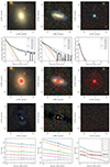 |
Fig. 2. Optical RGB image (top) of an inactive galaxy (left) and a low-redshift X-ray detected AGN (middle) and a QSO (right). Second row: Azimuth profile of the sources, with over-plotted available model profiles (PSF, REX, EXP, DEV, and SER). Third row: Apertures within which ap_flux[band] is measured. Fourth row: the residual image after subtracting the best model. Bottom row shows, within each aperture, all the colors computed; the figures show how the profiles of the colors change with the distance from the center, depending on the source type (see more details in the main text). |
In summary, the features extracted from LS10 and considered in this work are:
FLUX_[band], FLUX_IVAR_[band], FLUX_res_[band]: these are the fluxes, inverse variance, and residuals, measured assuming the best model profile; APFLUX_[band], APFLUX_IVAR_[band], APFLUX_res_[band]: these are the same as above but this time measured on the images, within various apertures; TYPE: the best model of the light profile. Originally this is a string that we converted to numeric.
dchisq13: Difference in χ2 between successively more complex model fits: PSF, REX, DEV, EXP, SER. The difference is versus no source. We then pre-processed the data by correcting the total and aperture fluxes for Galactic extinction14, and computed all possible colors, including colors within each aperture. We also computed the signal-to-noise ratio (S/N) as:
![Mathematical equation: $ \mathrm{S/N\_[band]} = \mathrm{FLUX\_[band]} \times \sqrt{\mathrm{(FLUX\_IVAR\_[band])}} $](/articles/aa/full_html/2024/10/aa50886-24/aa50886-24-eq1.gif) .
.
3. Training and blind samples
So far, unlike photo-zs computed via SED fitting, supervised machine learning algorithms (for example: regression or classification models that establish mappings from inputs to outputs) have been shown to be limited in their ability to extrapolate beyond the physical parameter space covered by the data they were trained on (see more details in Salvato et al. 2018a). Thus, their predictive accuracy may diminish significantly when applied to input values that lie well beyond patterns and ranges encountered during training and, therefore, rely extensively on the availability of a representative training sample (Newman & Gruen 2022). Various populations, such as star-forming galaxies, quiescent galaxies, or AGNs, exhibit unique physical attributes, highlighting the need for a thoughtful selection of tailored sources to be included in the training sample (Duncan et al. 2018). Given our objective to comprehensively explore the whole plethora of eROSITA-detected extragalactic populations, we have constructed a training sample that extensively covers the diversity in the AGN population. The training sample spans from low-luminosity, obscured, type II AGNs (Kauffmann et al. 2003; Laor 2008) to type I broad-line AGNs and quasars (Reynolds 1997; Richards et al. 2006), encompassing a wide redshift range, up to z = 6.6.
3.1. Construction of the sample for training
We are particularly interested in computing the photo-zs for X-ray-detected AGNs, particularly those detected by eROSITA. By nature of being all-sky, the eROSITA survey is shallower than the pencil-beam surveys conducted with XMM and Chandra, resulting in a sample less representative of galaxy-dominated and obscured AGNs and richer in bright and nearby, resolved AGNs. For this reason, we created the training sample by combining sources from eROSITA/eFEDS (Salvato et al. 2022) and 4XMM (Webb et al. 2020) for which reliable multi-wavelength counterparts from LS10 have been identified following the same procedure described in Sect. 3.1 and Appendix A of Salvato et al. (2022) for 3XMM.
The counterparts to the training sample are then matched in right ascension and declination (max separation of 1 arcsecond) with a compilation of spectroscopic redshifts available within the eROSITA collaboration. At this stage, the compilation is a mere list of catalogs from the literature collated. It encompasses approximately 13 million celestial sources, thus including duplicates and contradicting redshift measurements (see Kluge et al. 2024, for more details). Additionally, we extend the compilation by incorporating QSOs with reliable redshifts from the low-resolution spectra in Gaia DR3 (flagQSOC = 0 Gaia Collaboration 2023). For some sources, multiple spectroscopic matches are available, with discordant results. This can occur, for example, due to wrong line identification in low-S/N spectra. Here, we prioritize redshifts from eFEDS (Aydar et al., in prep.), given that most have all been visually inspected. Alternatively, a single entry is randomly selected, provided that the difference in spectroscopic redshift between the smallest and largest redshift entry Δz does not exceed Δz> 0.05. Objects failing to meet this criterion (≤0.3% of cases) are excluded from consideration to avoid the accidental assignment of incorrect redshift values to objects in the training sample. Objects with spectroscopic matches falling within the redshift range of z≤ 0.002 are assumed to be galactic and, therefore, excluded from any further consideration. The compilation is enriched by including 152 proprietary entries from SDSS-V (Kollmeier et al., in prep.) (SPECPRIMARY == 1, ZWARNING == 0). Within SDSS-V, the Black Hole Mapper (BHM, Anderson et al., in prep) is one of the primary surveys, specializing in long-term, time-domain investigations of AGNs and the optical characterization of eROSITA X-rays sources detected during the initial 1.5 years of the all-sky survey. This part of the training sample is represented in the histogram of Fig. 3 with a solid violet line.
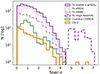 |
Fig. 3. Redshift distribution of the training (violet) and the blind samples (CSC2 in orange; Chandra-COSMOS Legacy in green). The distribution of the training sample is split between sources from 4XMM, eROSITa/eFEDS, and high-z sources from Fan et al. (2023). |
3.2. Extension of the training sample to high-z sources
The contribution to the high-redshift AGN population at z > 5 from X-ray pencil-beam surveys is feeble 15. By construction, the training sample would not represent the high-z population. However, eROSITA is expected to detect about 90 sources at z > 5.5 by the end of the mission (Wolf et al. 2021). At the same time, about a dozen have already been identified (Medvedev et al. 2020, 2021; Wolf et al. 2021, 2023, 2024). The optical spectra of these high-z QSOs closely resemble the spectra of QSOs at low redshift (for example Mortlock et al. 2011; Yang et al. 2021), which is why we have extended the training sample, adding 283 sources spectroscopically confirmed at z > 5.5, from the compilation of Fan et al. (2023), regardless of whether or not they are detected in the X-rays. The violet dashed histogram in Fig. 3 shows the redshift distribution of these sources.
3.3. Samples for blind tests
In addition to the sample that will be partitioned in training, test, and validation (see Sect. 4.2), we want to blindly test the consistency of the results obtained by CIRCLEZ for two additional samples:
CSC2: This blind sample is generated using the counterparts to the CSC2 objects16 in the same way as was done for the training sample. The original sample of CSC2 sources with reliable counterparts included 5643 sources. Screening for sources with spectroscopic redshift and after removing the sources that are in common with the training sample, 413 remain in the area covered by LS10-South, after including 26 redshifts from SDSS-V.
Chandra-COSMOS Legacy: For the counterparts to the X-ray sources presented in Marchesi et al. (2016), we consider the corresponding LS10 source using a match in coordinates (max separation of 1 arcsec). We then matched the sources to the compilation of redshifts available within the COSMOS collaboration (Khostovan et al., in prep), considering only reliable redshifts (Flags 3, 4, 13, and 14). After removing the sources common to the training sample, 1699 sources are considered.
Table 2 and Fig. 3 show the final composition of the sample for training and blind samples as well as the source distribution in redshift, respectively. Figure 4 shows the distribution of the sources considered in this paper in the X-rays flux and W1 magnitude plane, as defined in Salvato et al. (2018b). The redshift range of CSC2 and Chandra-COSMOS are well represented by the sample used for training which matches CSC2 also in the W1 and X-rays flux of CSC2. Unlike CSC2, the bulk of the sources in the Chandra-COSMOS sample are much fainter than the training sample in both X-rays and W1 (see Fig. 3).
Sources used in this work.
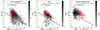 |
Fig. 4. X-rays flux vs. W1 magnitude distributions for the training (left panel) and the blind samples: CSC2 (middle panel) and Chandra-COSMOS (right panel). The dashed line represents the galactic/extragalactic separation proposed in Salvato et al. (2018b), who already pointed out that bright nearby galaxies would be misclassified. The contours encompassing 50%, 80%, and 95% of the training sample distribution are over-plotted on all panels. While the CSC2 sample has a distribution similar to the training sample, the distribution of the Chandra-COSMOS Legacy sources is biased toward fainter values of X-rays and W1. |
4. The method
This section describes our machine learning method and uncertainty quantification technique.
4.1. Problem formulation
We denote the input data as 𝒟 := {X, Y}, where X ∈ ℝM × N is the feature matrix with M features for N sources that we have discussed in Sect. 2 and Y ∈ ℝN represents the corresponding labels, which in our case, are given by spectroscopic redshifts. We denote the probability density function (PDF) of the normal distribution with mean μ and variance σ as  . A supervised learning approach to photo-zs would typically be tasked to find a parameterized function fθ : ℝM ↦ ℝ, which, given the photometry-based input features, predicts the redshift. The function may be a neural network, which typically is trained to minimize a loss function based on a training sample.
To illustrate our more general approach, we first consider a simpler case. We assume that the conditional predictive distribution is represented by a Gaussian distribution with fixed, data-independent variance α2 and mean y given by the neural network:
 (1)
(1)
where α2 is the variance and  is the predicted redshifts.
The free parameters of the network are then constrained by minimizing the Negative Log Likelihood (NLL) of predicting the spectroscopic redshift given the input photometry. This minimization problem is equivalent to minimizing the square of the difference,
 (2)
(2)
between the predicted redshifts,  , and the ground truth, y, a secure spectroscopic redshift. During inference, the mode (which in the case of Gaussian is also the mean) of the conditional predictive distribution is typically reported as the predicted solution. The variance of the Gaussian distribution remains constant regardless of the input data during the inference phase, leading to miss-calibrated uncertainty estimation. Moreover, a Gaussian probability distribution quantifying the redshift uncertainty is too restrictive. Due to potential color-redshift degeneracies (for example, Fig. 1 in Salvato et al. 2018a), the conditional predictive distribution is, in many cases, better described with a multi-modal distribution. To address this, D’Isanto et al. (2018) adopted convolutional neural networks (CNNs) combined with a mixture density network (MDN) to predict conditional predictive distributions based on multi-band imaging data.
We use a parameterized Gaussian mixture to describe the hypothesis class of the conditional predictive distribution, namely:
 (3)
(3)
However, as shown in D’Isanto et al. (2018), a single trained network producing a PDF cannot capture the uncertainty. We, therefore, extended our approach for uncertainty estimation and followed Lakshminarayanan et al. (2017) who proposed to use an ensemble of deep neural networks such as MDNs to improve uncertainty estimates. We follow this approach with an ensemble of MDNs that, given the photometric input features, each predicts the parameters of the Gaussian mixture distribution with a certain number of components. To be specific, the ith model fi(x; θi) in an ensemble of N models, given its parameters θi and the input features x, predicts the parameters of a Gaussian mixture composed of ni Gaussian, defined by the means μi(x; θi), and standard deviations σi(x; θi) and weights ωi(x; θi). The conditional predictive distribution defined by this MDN is given by:
 (4)
(4)
Finally, the predictions from all models are combined to give the posterior as
 (5)
(5)
For simplicity, the models are combined with equal weights. Each network in the ensemble is trained (see Sect. 4.2) independently, minimizing a suitable loss function (see Sect. 4.2.1). The hyper-parameters of this approach include the number of trained models to combine and the number of Gaussian components for each model, ni. The training conditions and model hyperparameters, including the number of Gaussians, are set differently for every network in the ensemble, and the training is described in Sect. 4.2.2. As shown in Eq. (5), the predictions of the individual models in the ensemble are combined equally to give the resulting conditional predictive distribution, which is also a mixture of Gaussians. The post-processing steps to summarize the resulting PDF, including identifying the mode, mean and uncertainties, are given in Sect. 4.2.3.
4.2. Training and inference pipeline
We partition the samples into training, validation, and test splits roughly with proportions 80: 10: 10. We use the training split to train the model across different combinations of the hyperparameters. The model’s performance on the validation split is evaluated to find suitable model architectures and training conditions, including parameter initialization, arguments for the optimizer, loss function, and others. A visualization of the general pipeline that takes the input catalog and returns a parameter representation of the posterior is depicted in Fig. 5. Among all features, we treat the vectorized morphological “TYPE” separately. Initially, this feature is transformed into a one-hot vector before applying a learnable linear transformation to embed them into ℝn, where we treat n as a hyperparameter. For the rest of the features, we compute and store the mean and the standard deviation on the train and validation splits of the data and use them to normalize individual features. We utilized the identical mean and standard deviation values employed during the training phase for feature normalization during inference.
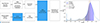 |
Fig. 5. Training and inference pipeline. The blue boxes show the trained aspects of the model. We have intentionally chosen a complex posterior to demonstrate features. In most cases, posteriors produced by the model are close to a single Gaussian with a clear mono-modal prediction. |
We employed a fully connected neural network to predict the distribution parameters from the concatenated feature representation. In the following subsections, we discuss our choice of loss functions, training procedure, and post-processing the inference on new samples.
4.2.1. Loss functions
In the case of standard regression, we can find the network parameters as an approximation to the maximum likelihood estimate (MLE) by minimizing the NLL loss. NLL loss can also be used for mixture density networks. Additionally, we implemented the continuous ranked probability score (CRPS) as done by D’Isanto et al. (2018), which compares the cumulative distribution function (CDF) of the predicted distribution against the Heavyside function, where the step is located at a value given by the ground truth; namely, the spectroscopic redshift. If we let Fx be the CDF of the conditional predictive distribution given the input x and ground truth y; then the CRPS loss is defined as
 (6)
(6)
Let pθ(y|x) be the predicted distribution and q(y|x) represent the true conditional distribution17, given y|x ∼ q(y|x), the scoring rule S(pθ, y|x) evaluates the quality of the predicted posterior in regards to the sample y|x. Higher values represent better alignment with the true posterior q(y|x). The expected scoring rule concerning the true distribution can further be evaluated as:
![Mathematical equation: $$ \begin{aligned} (p_\theta ({ y}|x), q({ y}|x)) = \mathbb{E} _{{ y}|x \sim q({ y}|x)}[S(p_\theta ({ y}|x), { y}|x)]. \end{aligned} $$](/articles/aa/full_html/2024/10/aa50886-24/aa50886-24-eq11.gif) (7)
(7)
CRPS and NLL are proper scoring rules; namely, they are optimal when the predicted conditional distribution is the same as the true conditional distribution. The latter can be shown to satisfy this property using Gibb’s inequality as done in Lakshminarayanan et al. (2017), while the CRPS loss is shown to be a proper scoring rule in Gneiting & Raftery (2007).
4.2.2. Training procedure and hyperparameter search
The space of models that we considered is determined by the hyperparameters described in Table 3. We employed the normal Xavier initialization to initialize the network’s parameters (namely weights), treating its parameters as hyperparameters. To find the most suitable network parameters, we minimized the loss functions described in Sect. 4.2.1 together with the L2 regularization. We used the ADAM optimizer (Kingma & Ba 2017) along with a learning rate schedule. We randomly select hyperparameters concerning the model, optimizer, and scheduler for both loss functions for each configuration. We saved the trained model if the corresponding loss on the validation samples is lower than a threshold. Upon randomly selecting the model architecture and training conditions, we gathered ∼36 models each while optimizing for NLL and CRPS losses.
Model and training hyperparameters with the range within which they are selected.
4.2.3. Inference and post-processing
To predict the distribution for new samples, we combined the models’ results uniformly as discussed in Sect. 4.1. We compared the results evaluated on the validation and test merged samples for the combination of the models trained on CRPS loss and those trained on NLL loss in Table 4. We performed slightly better by combining CRPS and NLL models than by considering models trained on individual loss functions (see Table 4). The resulting posterior of the ensemble has 184 Gaussian (GMM) in the mixture.
Averaged statistics across all individually trained NLL loss and CPRS models.
To obtain a point estimate of the redshift, we find the mode of the resulting Gaussian distribution because the mean or median could be misleading for bi- or multi-modal distributions. In addition to the point estimates, we provide the redshift posterior for all sources computed as the sum of the Gaussian distributions in the GMM. We provide this in the form of a set of posterior values for 2000 points linearly spaced in the range (0 < z < = 7)18. We also provide the upper and lower 1σ and 3σ errors from the posterior. We do this by finding the values where the cumulative distribution function is equal to the equivalent 1σ and 3σ probabilities of a normal distribution (see the left panel of Fig. 5 for a schematic representation).
5. Redshift computation for eFEDS sources and comparison with literature
Using the model prediction described in Sect. 4 we have extended the computation of redshift to the 22 079 sources in the eROSITA/eFEDS catalog of counterparts (Salvato et al. 2022) that have been classified as extragalactic (CTP_CLASS> 2), using only LS10-South data. For the eFEDS sources in the test and validation sample the comparison between the spectroscopic redshift and the photo-z computed with CIRCLEZ is shown in Fig. 6. As a reminder, Salvato et al. (2022) presented two different methods of computing photo-zs, one based on SED fitting LEPHARE and one based on machine learning DNNZ, the latter also based on CNN and with an architecture very similar to the one of CIRCLEZ. In particular, in Salvato et al. (2022), the metrics (accuracy and fraction of outliers) were split into three distinct regions based on the photometry quality. Region 1, centered on the GAMA09 field, has the best data, including optical data from HSC, optical and near-infrared (NIR) data from KiDS-Viking, optical and MIR data from LS8, and UV from GALEX. This is the region where LEPHARE performed best. In Region 2, there is a drop in accuracy and an increase in the fraction of outliers due to the lack of deep near-infrared data and probably some issue with the calibration of the r and i band in HSC. The latter is suggested by the fact that DNNZ follows a similar trend and has a drop in the accuracy and the fraction of outliers in Region 2, as LEPHARE, despite relying only on HSC data. Region 3 is the region where data are very pure in general and not considered further in the comparison.
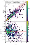 |
Fig. 6. Comparison between photo-z computed with CIRCLEZ and spectroscopic redshifts in eFEDS, considering only the test and validation sources. |
The metrics (this time also including bias) for Regions 1 and 2 for LEPHARE and DNNZ are reported in Table 5 for comparison, together with the same metrics computed using CIRCLEZ for the sources in eFEDS that are part of the training, test, validation samples, and overall. By comparing the metrics, it is clear that the new photo-z are superior to those previously available for that area, despite relying only on optical and mid-infrared data from LS10. The accuracy is slightly worse than for DNNZ, in general, and LEPHARE in Region 2. However, the fraction of outliers has noticeably dropped for all samples. The bias is also slightly worse than for DNNZ and LEPHARE in Region 1, but comparable for Region 2. Region 1 is the area with the reacher, deeper, and more homogenous photometry from KiDS and HSC (see Salvato et al. 2022, for details).
It is also worth mentioning that the metrics reported for LEPHARE and DNNZ were measured using the training sample, not on the test and/or validation sample. If we compute the metrics for CIRCLEZ using all the spectroscopy, namely including those used for the training and validation, the values would suggest a quality close to the one available for the best pencil-beam surveys (XMM-COSMOS, (E)CDF Salvato et al. 2009; Luo et al. 2010; Hsu et al. 2014), computed with deep, rich and homogenized photometry). This assures that the new photo-zs made available for eFEDS in this paper are reliable and can be used for luminosity function studies or for preselecting specific instruments or wavelengths of interest when submitting a proposal.
The new photo-zs also provide more realistic PDZ, 1 and 3σ errors. In fact, it is well known that SED fitting tends to underestimate the errors. Usually, the fraction of sources with spectroscopic redshift within 1σ from the photometric ones is very low (for example, Dahlen et al. 2013). The area within the photo-zs and /pm 0.1 of the PDZ (PDZ_BEST in LEPHARE) is usually taken as a measure of the reliability of the photo-zs. When PDZ_BEST is high, the solution is very peaked, while a low PDZ_BEST indicates large uncertainties and degeneracy of the solutions. In Brescia et al. (2019), it was shown that for the AGN in STRIPE82-X (Ananna et al. 2017), the PDZ_BEST was high for many outliers. Figure 7 shows this fraction in bins of redshift for LEPHARE, DNNZ, and CIRCLEZ applied to eFEDS. CIRCLEZ and DNNZ perform better than LEPHARE, with CIRCLEZ performing better overall at z> 2.
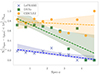 |
Fig. 7. Fraction of sources with spectroscopic redshift within 1σ from the photo-zs, in eFEDS. In addition to the trend per bin (crosses, filled dots, and squares), we plot the regression fits (dashed line) as well as 95% confidence intervals (shaded regions). |
Together with this paper, we have released a new catalog of photo-z computed with CIRCLEZ, for the extragalactic sources in the eROSITA/eFEDS field. For each source we provide, in addition to the eROSITA_ID, the photo-z, and the 1 and 3 σ lower and upper errors, also a unique identifier for the counterpart in the LS10 catalog. The identifier is created by concatenating the columns RELEASE, BRICKID, and OBJID. In addition, we provide about 5000 new spectroscopic redshifts that became available with the 18th Data Release of SDSS-V (Almeida et al. 2023). The catalog is available via Vizier and on the eROSITA/EDR page19
6. Robustness tests
Almost 60% of the training samples’ sources are from eFEDS, where the X-ray observations and the LS10 photometry are homogeneous. Then, we could argue that the quality of the photo-z is field-dependent. To check the robustness of CIRCLEZ we computed photo-z for the two blind samples presented in Sect. 3.3. The results on various metrics are reported in Table 5. First, we applied CIRCLEZ on the CSC2 sample, which has a distribution in X-ray and W1 flux similar to the training sample. Unsurprisingly, η and σNMAD are comparable to those obtained for the training and validation sample (see the left panel of Fig. 8).
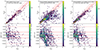 |
Fig. 8. CIRCLEZ photo-zs vs spectroscopic redshifts for the CSC2 sample (left panel) and Chandra-COSMOS Legacy sample from Marchesi et al. (2016) (middle and right panel). Numbers in the figures show the number of objects visible in this redshift range instead of the full sample number. In Chandra-COSMOS, the performance is reduced due to the increased faintness of the survey and, therefore, fainter counterparts. |
The middle and right panels of the same figure show the performance on the Chandra-COSMOS sample of Marchesi et al. (2016). As expected, the performance for this faint sample is dramatically reduced compared to the X-rays brighter eFEDS sample, given that the counterparts for these fainter X-ray sources will also have faint photometry and thus lower S/N in the shallow LS10 survey. However, if we limit the sample to sources brighter than about 21 magnitudes (see Table 5), the quality of the photo-z is consistent with previous results, suggesting that we are limited only by the depth of the data.
6.1. PIT score
For scientific exploitations, in addition to a point prediction, reliable errors must be provided by any photo-z tool. In particular, the full posteriors to reflect our knowledge of the redshift is needed, for example, in the computation of luminosity functions (for example, Buchner et al. 2015; Fotopoulou et al. 2016; Miyaji et al. 2015). For this reason, we also looked at the probability integral transform (PIT: D’Isanto et al. 2018; Schmidt et al. 2020) for all three samples. The PIT value is the integral of the posterior up to the spectroscopic redshift (see the left panel of Fig. 5) and would be uniformly distributed if the spectroscopic redshifts were drawn from the posteriors. The results for the test sample in eFEDS, CSC2, and Chandra-COSMOS are shown in Fig. 9. The quantile-quantile plots show the PIT value against a uniformly distributed value. The figures were produced using the Redshift Assessment and Infrastructure Layers (RAIL) framework, discussed in detail in Schmidt et al. (2020). The figure demonstrates the overall good performance of the posterior distribution and the point prediction performance. It demonstrates that the full posteriors are neither overly nor underly dispersed for eFEDS and CSC2. If the spectroscopic samples were drawn from the posterior, the PIT distribution would be uniform. An excess of PIT values at the lower or upper ends shows that the posteriors are not identifying true values at their lower or upper ends, as it is happening for Chandra-COSMOS. An excess in the center shows that the posteriors are underdispersed and underestimate the errors on the point predictions.
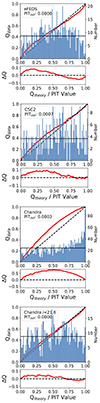 |
Fig. 9. PIT distribution and quantile-quantile plot between photo-z computed with CIRCLEZ and the spectroscopic redshifts for the test and validation sources in eFEDS (top panel), CSC2 (second row) and Chandra-COSMOS Legacy without (third row) and with a cut in magnitude (bottom panel). While the first two samples perform well, the PIT distribution for Chandra-COSMOS is in excess of the upper end. |
6.2. Limitations on photo-zs for all-sky surveys
To further test the robustness of CIRCLEZ, in Fig. 10, we plotted the photo-z computed in eFEDS and the width of the 1σ error, color coding the sources as a function of their magnitude. The scatter plot is broad, but a sharp line delimits the smaller error associated with the photo-z, corresponding to the brighter sources. The brightest sources typically also have smaller photometry uncertainties (and thus a high S/N) and, thus, more accurate photo-zs. As it is visible in Fig. 1, the depth of LS10 is not homogeneous, implying that the quality of the photometric redshifts for all-sky surveys, such as eROSITA, will have various grades of accuracy. However, the PIT score analysis on CSC2 (random distribution in the sky) demonstrated that the PDZs correctly account for this limitation.
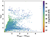 |
Fig. 10. Photo-z vs 1σ error for all the sources in eFEDS with spectroscopic redshift available, color-coded by their magnitude in the r band. |
7. Discussion
Thus far, there has been scant optimism regarding the feasibility of attaining accurate photo-zs for AGNs in all-sky surveys. This was due to the assumption that many photometric bands from different surveys needed to be assembled and cross-calibrated (unthinkable to be achieved for wide areas). It remains true that a larger number of bands makes it easier to describe the SED of these complex sources; however, in this work, we have demonstrated that using an adequate training sample and going beyond the use of fluxes and colors with a machine learning approach, reliable photo-zs can be achieved for the first time, using only optical and WISE data as offered by LS10-South. In particular, the features include information on the light distribution of the sources, parameterized by the fluxes and colors for different apertures, and the quality of the fit assuming different morphological types, in addition to photometric errors and tractorized (Lang 2014) WISE photometry.
It is important to stress that there is room for improvement in what LS10 provides. As measured by LS10, the photometry within apertures does not account for the additional flux emitted by neighbor sources. We tested whether this could explain at least some of the outliers. For that, we identified the neighbors within 5" from all eFEDS sources with spectroscopy. We then considered the brightest of the neighbors and the magnitude difference from the central source (Δmag). We categorized the neighbors into classes based on their relative brightness: “isolated” (no neighbor), “more than 3 magnitudes dimmer”, “between 3 and 1 magnitude dimmer”, “between 1 magnitude dimmer and 1 magnitude brighter”, “between 1 and 3 magnitudes brighter” and “more than 3 magnitudes brighter”. These criteria must be met in all 4 optical bands g, r, i and z. Imposing the same trend in all bands reduces the sample that can be analyzed, but in return, we get a clearer correlation. In Fig. 11 we report the mean value of the outlier fraction for the sources in various bins of Δmag, indicating with a red dashed line the outliers fraction for the isolated eFEDS sources sample. Sources with no neighbors or very faint neighbors have a lower fraction of outliers, which increase with the increasing brightness of the neighbors. This implies that the quality of the photo-zs could improve further if the Imaging Legacy Survey for DESI would consider providing a segmentation map for redefining the area to be used for measuring the aperture fluxes (for example, SeXseg, Coe 2015) in their future data releases. More on this will be discussed in Roster et al. (in prep.), where photo-zs for AGNs are computed using directly the images.
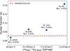 |
Fig. 11. Outlier fraction as a function of binned relative neighbor brightness. The outliers increase in the presence of bright neighbors. |
Currently, LS10 is the only survey that provides this kind of information, and we argue here that surveys such as the Legacy Survey of Space and Time (LSST; Ivezić et al. 2019b) and Euclid (Euclid Collaboration 2024) should provide the same kind of output. The Vera C. Rubin Observatory will utilize the pipeline already tested on Hyper Suprime Cam and presented in Bosch et al. (2018). The plan20 is for the pipeline to provide fluxes for several concentric apertures, together with total flux and errors assuming two best-fitting models: a PSF and a composite bulge+disk model. The multi-epoch observations with LSST will also help improve photo-zs for AGNs in two ways. First, a correction for variability could be applied to the photometry as already successfully implemented in Salvato et al. (2009). Second, variability is at least in part also redshift-dependent (Satheesh-Sheeba et al., in prep.).
Euclid would offer further constraining power due to its exceptional spatial resolution and wavelength coverage extending to NIR photometry. However, no plans exist to provide aperture photometry in multiple annuli as part of the standard data release products Merlin et al. (2019). Guy et al. (2022) recommends the joint processing of Rubin and Euclid data products, including aperture fluxes and other measures. A high density of apertures could significantly impact photometric redshift performance using the method presented here and add significant value to the resultant data sets. However, there is currently no plan for both surveys to combine their photometry with WISE. At the same time, the analysis of the features presented in Table A.1 suggests that the features from WISE are key in all analyzed subgroups.
8. Conclusions and summary
In this paper, we present CIRCLEZ, a new algorithm for estimating redshifts for AGNs. The model is based on FCNN21, applied to aperture photometry from optical to MIR data from LS10-South, already publicly available over the entire footprint of eROSITA-DE. For this purpose, we have constructed a sample of 14173 sources of X-ray-detected AGNs enriched by a sample of 391 AGNs at high-z to be used as training, test and validation samples (see Sect. 3). We did not limit the features to those expressing total fluxes (together with their errors) and colors, as is usually done in SED fittings. Instead, we considered all features that are (at least at some level) redshift-dependent (see Appendix A). These features are related to the light profile of the galaxies and the apparent host-and-AGN relative contribution and are described in Sect. 2 and Fig. 2. In short they are fluxes within various apertures, corrected for Galactic extinction, from which also colors within annuli are computed. In addition, we considered the quantity “dchisq” which expresses how closely the azimuth profile of a source resembled the PSF, DEV, REX, and SER model profiles. All the features are either already offered in the standard LS10 catalog or easily computed from the available columns.
The model obtained in the training was then applied to the eROSITA/eFEDS field (Sect. 5). Overall, we have obtained a comparable or better quality photo-z to what was previously available in the best region of the field (REGION 1), with much less effort than in the process described in Salvato et al. (2022), despite lacking UV, u and NIR band photometry. Together with this paper, we have released a new catalog of photo-zs in eFEDS, including 1 and 3σ errors and PDZ (end of Sect. 5).
We tested the stability of the results (Sect. 3.3) by using CIRCLEZ and the model obtained in the training phase on two additional samples, used for a blind test. The first sample, formed by 651 sources from CSC2 in the footprint of LS10-South, shares the same properties (in terms of WISE and X-ray fluxes) as the training sample. There, the quality of the photo-zs is consistent with the one obtained in the validation sample limited to eFEDS sources. The second blind sample consists of all the AGNs detected in the Chandra-COSMOS Legacy survey, with reliable spectroscopic redshift and detected in t LS10-South. The metrics indicate that the quality of the photo-zs is consistent with the one computed in the test sample of eFEDS and in CSC2, as long as we consider a limiting AB magnitude of 21.7 in the i band. The accuracy degrades rapidly for fainter sources (and thus with larger photometric errors).
This implies that the method is stable and reliable, and what is now needed for computing reliable photo-zs for AGNs in all-sky surveys is photometry computed as in LS10 but at a deeper depth over the entire sky. Future deep photometric surveys such as LSST and Euclid, given that they will allow us to identify the faint and high-z AGNs, should consider providing the same quantities provided by LS10, including the WISE photometry matched and de-blended with respect to the optical data. More information on morphological and spatial properties will improve not only photo-zs, but also the classification and identification of AGNs, as was previously demonstrated in Doorenbos et al. (2022), Savić et al. (2023). Ideally, both surveys should provide the photometry in various apertures, after masking nearby objects (this is a current limitation in the data provided by LS10). While deeper data will improve the quality of photo-zs for faint and high-z AGNs, a further improvement will also come from the increasing training sample size, thanks to the Black Hole Mapper (BHM) programs at SDSS-V and 4MOST, which focus on AGN spectroscopic and on the follow-up of eROSITA X-ray sources. Altogether, the surveys will provide spectroscopic redshifts with completeness of > 60% down to the r magnitude of 21.5 and 22.5 for the eRASS:3 and eRASS:5, respectively, for a total of about one million22 sources.
See Sect. 7.2 of Salvato et al. (2022), and Table 5 of this paper, where the quality of the photo-zs in the area within and outside the homogenized optical-NIR photometry from KiDS (Kuijken et al. 2019) is compared.
Comparison of bias, fraction of outliers, and accuracy between photo-z computed with CIRCLEZ, LEPHARE, and DNNZ, for extragalactic sources in the eROSITA/eFEDS field.
Flux measured within a circular aperture whose radius is defined by the shape of the azimuthally averaged light profile.
η = |zphot − zspec|> 0.15 ⋅ (1 + zspec).
σNMAD = 1.48 ⋅ median((zphot − zspec)/(1 + zspec)).
Updated results from the same authors using LS10 are described at https://www.legacysurvey.org/dr10/files/#photo-z-sweeps-10-1-photo-z-sweep-brickmin-brickmax-pz-fits
Meant here as an extension in images and classification.
The complete list of parameters and their description are available at https://www.legacysurvey.org/dr10/catalogs/
More details are available at https://www.legacysurvey.org/dr10/catalogs/
We follow the recipe provided by the LS10 team: Flux_[band]/MW_transmission_[band], with MW_transmission_[band] also available in the LS10 catalog.
Unsurprisingly, most of the sources at redshift higher than five that we visually inspected were wrong.
Assume that the data  comes from some distribution
  with the corresponding true conditional distribution q(y|x).
We also provide the GMM values so the user can recompute on a different grid if preferred.
https://erosita.mpe.mpg.de/edr/eROSITAObservations/Catalogues/. The redshift probability function (PDZs) for each source is also available, under request.
Fully connected neural network.
Acknowledgments
We thank the referee for their careful reading of the manuscript and the constructive feedback. MS thanks Dr. Marianna Lucio for the insights on features analysis and statistics. Part of this work was supported by the German Deutsche Forschungsgemeinschaft, DFG project Funded by Deutsche Forschungsgemeinschaft (DFG, German Research Foundation) under Germany’s Excellence Strategy – EXC 2094 – 390783311. CR acknowledges support from Fondecyt Regular grant 1230345 and ANID BASAL project FB210003. RJA was supported by FONDECYT grant number 1231718 and the ANID BASAL project FB210003. This work is based on data from eROSITA, the soft X-ray instrument aboard SRG, a joint Russian-German science mission supported by the Russian Space Agency (Roskosmos), in the interests of the Russian Academy of Sciences represented by its Space Research Institute (IKI), and the Deutsches Zentrum für Luft- und Raumfahrt (DLR). The SRG spacecraft was built by Lavochkin Association (NPOL) and its subcontractors and is operated by NPOL with support from the Max Planck Institute for Extraterrestrial Physics (MPE). The development and construction of the eROSITA X-ray instrument were led by MPE, with contributions from the Dr. Karl Remeis Observatory Bamberg & ECAP (FAU Erlangen-Nuernberg), the University of Hamburg Observatory, the Leibniz Institute for Astrophysics Potsdam (AIP), and the Institute for Astronomy and Astrophysics of the University of Tübingen, with the support of DLR and the Max Planck Society. The Argelander Institute for Astronomy of the University of Bonn and the Ludwig Maximilians Universität Munich also participated in the science preparation for eROSITA. The Legacy Surveys consist of three individual and complementary projects: the Dark Energy Camera Legacy Survey (DECaLS; Proposal ID 2014B-0404; PIs: David Schlegel and Arjun Dey), the Beijing-Arizona Sky Survey (BASS; NOAO Prop. ID 2015A-0801; PIs: Zhou Xu and Xiaohui Fan), and the Mayall z-band Legacy Survey (MzLS; Prop. ID 2016A-0453; PI: Arjun Dey). DECaLS, BASS, and MzLS together include data obtained, respectively, at the Blanco telescope, Cerro Tololo Inter-American Observatory, NSF’s NOIRLab; the Bok telescope, Steward Observatory, University of Arizona; and the Mayall telescope, Kitt Peak National Observatory, NOIRLab. Pipeline processing and analyses of the data were supported by NOIRLab and the Lawrence Berkeley National Laboratory (LBNL). The Legacy Surveys project is honored to be permitted to conduct astronomical research on Iolkam Du’ag (Kitt Peak), a mountain with particular significance to the Tohono O’odham Nation. NOIRLab is operated by the Association of Universities for Research in Astronomy (AURA) under a cooperative agreement with the National Science Foundation. LBNL is managed by the Regents of the University of California under contract to the U.S. Department of Energy. This project used data obtained with the Dark Energy Camera (DECam), which was constructed by the Dark Energy Survey (DES) collaboration. Funding for the DES Projects has been provided by the U.S. Department of Energy, the U.S. National Science Foundation, the Ministry of Science and Education of Spain, the Science and Technology Facilities Council of the United Kingdom, the Higher Education Funding Council for England, the National Center for Supercomputing Applications at the University of Illinois at Urbana-Champaign, the Kavli Institute of Cosmological Physics at the University of Chicago, Center for Cosmology and Astro-Particle Physics at the Ohio State University, the Mitchell Institute for Fundamental Physics and Astronomy at Texas A & M University, Financiadora de Estudos e Projetos, Fundacao Carlos Chagas Filho de Amparo, Financiadora de Estudos e Projetos, Fundacao Carlos Chagas Filho de Amparo a Pesquisa do Estado do Rio de Janeiro, Conselho Nacional de Desenvolvimento Cientifico e Tecnologico and the Ministerio da Ciencia, Tecnologia e Inovacao, the Deutsche Forschungsgemeinschaft and the Collaborating Institutions in the Dark Energy Survey. The Collaborating Institutions are Argonne National Laboratory, the University of California at Santa Cruz, the University of Cambridge, Centro de Investigaciones Energeticas, Medioambientales y Tecnologicas-Madrid, the University of Chicago, University College London, the DES-Brazil Consortium, the University of Edinburgh, the Eidgenossische Technische Hochschule (ETH) Zurich, Fermi National Accelerator Laboratory, the University of Illinois at Urbana-Champaign, the Institut de Ciencies de l’Espai (IEEC/CSIC), the Institut de Fisica d’Altes Energies, Lawrence Berkeley National Laboratory, the Ludwig Maximilians Universitat Munchen and the associated Excellence Cluster Universe, the University of Michigan, NSF’s NOIRLab, the University of Nottingham, the Ohio State University, the University of Pennsylvania, the University of Portsmouth, SLAC National Accelerator Laboratory, Stanford University, the University of Sussex, and Texas A&M University. BASS is a key project of the Telescope Access Program (TAP), which has been funded by the National Astronomical Observatories of China, the Chinese Academy of Sciences (the Strategic Priority Research Program “The Emergence of Cosmological Structures” Grant # XDB09000000), and the Special Fund for Astronomy from the Ministry of Finance. The BASS is also supported by the External Cooperation Program of Chinese Academy of Sciences (Grant # 114A11KYSB20160057), and Chinese National Natural Science Foundation (Grant # 12120101003, # 11433005). The Legacy Survey team uses data products from the Near-Earth Object Wide-field Infrared Survey Explorer (NEOWISE), a project of the Jet Propulsion Laboratory/California Institute of Technology. NEOWISE is funded by the National Aeronautics and Space Administration. The Legacy Surveys imaging of the DESI footprint is supported by the Director, Office of Science, Office of High Energy Physics of the U.S. Department of Energy under Contract No. DE-AC02-05CH1123, by the National Energy Research Scientific Computing Center, a DOE Office of Science User Facility under the same contract, and by the U.S. National Science Foundation, Division of Astronomical Sciences under Contract No. AST-0950945 to NOAO. Funding for the Sloan Digital Sky Survey V has been provided by the Alfred P. Sloan Foundation, the Heising-Simons Foundation, the National Science Foundation, and the Participating Institutions. SDSS acknowledges support and resources from the Center for High-Performance Computing at the University of Utah. SDSS telescopes are located at Apache Point Observatory, funded by the Astrophysical Research Consortium and operated by New Mexico State University, and at Las Campanas Observatory, operated by the Carnegie Institution for Science. SDSS is managed by the Astrophysical Research Consortium for the Participating Institutions of the SDSS Collaboration, including Caltech, The Carnegie Institution for Science, Chilean National Time Allocation Committee (CNTAC) ratified researchers, The Flatiron Institute, the Gotham Participation Group, Harvard University, Heidelberg University, The Johns Hopkins University, L’Ecole polytechnique fédérale de Lausanne (EPFL), Leibniz-Institut für Astrophysik Potsdam (AIP), Max-Planck-Institut für Astronomie (MPIA Heidelberg), Max-Planck-Institut für Extraterrestrische Physik (MPE), Nanjing University, National Astronomical Observatories of China (NAOC), New Mexico State University, The Ohio State University, Pennsylvania State University, Smithsonian Astrophysical Observatory, Space Telescope Science Institute (STScI), the Stellar Astrophysics Participation Group, Universidad Nacional Autónoma de México, University of Arizona, University of Colorado Boulder, University of Illinois at Urbana-Champaign, University of Toronto, University of Utah, University of Virginia, Yale University, and Yunnan University.
References
- Abazajian, K. N., Adelman-McCarthy, J. K., Agüeros, M. A., et al. 2009, ApJS, 182, 543 [Google Scholar]
- Ahn, C. P., Alexandroff, R., Allende Prieto, C., et al. 2012, ApJS, 203, 21 [Google Scholar]
- Aihara, H., Arimoto, N., Armstrong, R., et al. 2018, PASJ, 70, S4 [NASA ADS] [Google Scholar]
- Almeida, A., Anderson, S. F., Argudo-Fernández, M., et al. 2023, ApJS, 267, 44 [NASA ADS] [CrossRef] [Google Scholar]
- Ananna, T. T., Salvato, M., LaMassa, S., et al. 2017, ApJ, 850, 66 [Google Scholar]
- Arnouts, S., Cristiani, S., Moscardini, L., et al. 1999, MNRAS, 310, 540 [Google Scholar]
- Bianchi, L. 2014, Ap&SS, 354, 103 [NASA ADS] [CrossRef] [Google Scholar]
- Bosch, J., Armstrong, R., Bickerton, S., et al. 2018, PASJ, 70, S5 [Google Scholar]
- Brescia, M., Salvato, M., Cavuoti, S., et al. 2019, MNRAS, 489, 663 [NASA ADS] [CrossRef] [Google Scholar]
- Brunner, H., Liu, T., Lamer, G., et al. 2022, A&A, 661, A1 [NASA ADS] [CrossRef] [EDP Sciences] [Google Scholar]
- Buchner, J., Georgakakis, A., Nandra, K., et al. 2015, ApJ, 802, 89 [Google Scholar]
- Cardamone, C. N., van Dokkum, P. G., Urry, C. M., et al. 2010, ApJS, 189, 270 [Google Scholar]
- Chen, H., Lundberg, S. M., & Lee, S.-I. 2022, Nat. Commun., 13, 4512 [NASA ADS] [CrossRef] [Google Scholar]
- Cirasuolo, M., Afonso, J., Bender, R., et al. 2011, The Messenger, 145, 11 [Google Scholar]
- Civano, F., Elvis, M., Brusa, M., et al. 2012, ApJS, 201, 30 [Google Scholar]
- Coe, D. 2015, Astrophysics Source Code Library [record ascl:1508.006] [Google Scholar]
- Croton, D. J., Springel, V., White, S. D. M., et al. 2006, MNRAS, 365, 11 [Google Scholar]
- Dahlen, T., Mobasher, B., Faber, S. M., et al. 2013, ApJ, 775, 93 [Google Scholar]
- de Jong, R. S. 2019, Nat. Astron., 3, 574 [NASA ADS] [CrossRef] [Google Scholar]
- Dey, A., Schlegel, D. J., Lang, D., et al. 2019, AJ, 157, 168 [Google Scholar]
- Dey, B., Andrews, B. H., Newman, J. A., et al. 2022, MNRAS, 515, 5285 [NASA ADS] [CrossRef] [Google Scholar]
- Di Matteo, T., Springel, V., & Hernquist, L. 2005, Nature, 433, 604 [NASA ADS] [CrossRef] [Google Scholar]
- D’Isanto, A., Cavuoti, S., Gieseke, F., & Polsterer, K. 2018, A&A, 616, A97 [NASA ADS] [CrossRef] [EDP Sciences] [Google Scholar]
- Doorenbos, L., Cavuoti, S., Longo, G., et al. 2022, ArXiv e-prints [arXiv:2211.05556] [Google Scholar]
- Duncan, K. J., Jarvis, M. J., Brown, M. J. I., & Röttgering, H. J. A. 2018, MNRAS, 477, 5177 [Google Scholar]
- Euclid Collaboration (Mellier, Y., et al.) 2024, A&A, in press, https://doi.org/10.1051/0004-6361/202450810 [Google Scholar]
- Fan, X., Bañados, E., & Simcoe, R. A. 2023, ARA&A, 61, 373 [NASA ADS] [CrossRef] [Google Scholar]
- Fotopoulou, S., Salvato, M., Hasinger, G., et al. 2012, ApJS, 198, 1 [Google Scholar]
- Fotopoulou, S., Buchner, J., Georgantopoulos, I., et al. 2016, A&A, 587, A142 [NASA ADS] [CrossRef] [EDP Sciences] [Google Scholar]
- Gaia Collaboration (Vallenari, A., et al.) 2023, A&A, 674, A1 [NASA ADS] [CrossRef] [EDP Sciences] [Google Scholar]
- Gneiting, T., & Raftery, A. E. 2007, J. Am. Stat. Assoc., 102, 359 [CrossRef] [Google Scholar]
- Guy, L., Cuillandre, J.-C., Bachelet, E., et al. 2022, https://doi.org/10.5281/zenodo.5836022 [Google Scholar]
- Hsu, L.-T., Salvato, M., Nandra, K., et al. 2014, ApJ, 796, 60 [Google Scholar]
- Ilbert, O., Arnouts, S., McCracken, H. J., et al. 2006, A&A, 457, 841 [NASA ADS] [CrossRef] [EDP Sciences] [Google Scholar]
- Ivezić, Ž., Kahn, S. M., Tyson, J. A., et al. 2019b, ApJ, 873, 111 [Google Scholar]
- Kauffmann, G., Heckman, T. M., Tremonti, C., et al. 2003, MNRAS, 346, 1055 [Google Scholar]
- Kingma, D. P., & Ba, J. 2017, arXiv e-prints [arXiv:1412.6980] [Google Scholar]
- Kluge, M., Comparat, J., Liu, A., et al. 2024, A&A, 688, A210 [NASA ADS] [CrossRef] [EDP Sciences] [Google Scholar]
- Kohavi, R. 1995, International Joint Conference on Artificial Intelligence, https://api.semanticscholar.org/CorpusID:2702042 [Google Scholar]
- Kuijken, K., Heymans, C., Dvornik, A., et al. 2019, A&A, 625, A2 [NASA ADS] [CrossRef] [EDP Sciences] [Google Scholar]
- Lakshminarayanan, B., Pritzel, A., & Blundell, C. 2017, arXiv e-prints [arXiv: 1612.01474] [Google Scholar]
- Lang, D. 2014, AJ, 147, 108 [Google Scholar]
- Laor, A. 2008, ApJ, 590, 86 [Google Scholar]
- Lawrence, A., Warren, S. J., Almaini, O., et al. 2007, MNRAS, 379, 1599 [Google Scholar]
- Levi, M., Bebek, C., Beers, T., et al. 2013, ArXiv e-prints [arXiv:1308.0847] [Google Scholar]
- Lundberg, S., & Lee, S.-I. 2017, arXiv e-prints [arXiv:1705.07874] [Google Scholar]
- Luo, B., Brandt, W. N., Xue, Y. Q., et al. 2010, ApJS, 187, 560 [NASA ADS] [CrossRef] [Google Scholar]
- Madau, P., & Dickinson, M. 2014, ARA&A, 52, 415 [Google Scholar]
- Marchesi, S., Civano, F., Elvis, M., et al. 2016, ApJ, 817, 34 [Google Scholar]
- McMahon, R. G., Banerji, M., Gonzalez, E., et al. 2013, The Messenger, 154, 35 [NASA ADS] [Google Scholar]
- Medvedev, P., Sazonov, S., Gilfanov, M., et al. 2020, MNRAS, 497, 1842 [Google Scholar]
- Medvedev, P., Gilfanov, M., Sazonov, S., Schartel, N., & Sunyaev, R. 2021, MNRAS, 504, 576 [CrossRef] [Google Scholar]
- Merlin, E., Pilo, S., Fontana, A., et al. 2019, A&A, 622, A169 [NASA ADS] [CrossRef] [EDP Sciences] [Google Scholar]
- Merloni, A., Lamer, G., Liu, T., et al. 2024, A&A, 682, A34 [NASA ADS] [CrossRef] [EDP Sciences] [Google Scholar]
- Miyaji, T., Hasinger, G., Salvato, M., et al. 2015, ApJ, 804, 104 [Google Scholar]
- Mortlock, D. J., Warren, S. J., Venemans, B. P., et al. 2011, Nature, 474, 616 [Google Scholar]
- Newman, J. A., & Gruen, D. 2022, ARA&A, 60, 363 [NASA ADS] [CrossRef] [Google Scholar]
- Ni, Q., Brandt, W. N., Chen, C.-T., et al. 2021, ApJS, 256, 21 [CrossRef] [Google Scholar]
- Nishizawa, A. J., Hsieh, B.-C., Tanaka, M., & Takata, T. 2020, ArXiv e-prints [arXiv:2003.01511] [Google Scholar]
- Norris, R. P., Salvato, M., Longo, G., et al. 2019, PASP, 131, 108004 [Google Scholar]
- Predehl, P., Andritschke, R., Arefiev, V., et al. 2021, A&A, 647, A1 [EDP Sciences] [Google Scholar]
- Reynolds, C. S. 1997, MNRAS, 286, 513 [NASA ADS] [CrossRef] [Google Scholar]
- Richards, G. T., Lacy, M., Storrie-Lombardi, L. J., et al. 2006, ApJS, 166, 470 [Google Scholar]
- Rozemberczki, B., Watson, L., Bayer, P., et al. 2022, The Shapley Value in Machine Learning [Google Scholar]
- Salvato, M., Hasinger, G., Ilbert, O., et al. 2009, ApJ, 690, 1250 [CrossRef] [Google Scholar]
- Salvato, M., Ilbert, O., Hasinger, G., et al. 2011, ApJ, 742, 61 [Google Scholar]
- Salvato, M., Buchner, J., Budavári, T., et al. 2018a, MNRAS, 473, 4937 [Google Scholar]
- Salvato, M., Ilbert, O., & Hoyle, B. 2018b, Nat. Astron., 3, 212 [CrossRef] [Google Scholar]
- Salvato, M., Wolf, J., Dwelly, T., et al. 2022, A&A, 661, A3 [NASA ADS] [CrossRef] [EDP Sciences] [Google Scholar]
- Savić, D. V., Jankov, I., Yu, W., et al. 2023, ApJ, 953, 138 [CrossRef] [Google Scholar]
- Schmidt, S. J., Malz, A. I., Soo, J. Y. H., et al. 2020, MNRAS, 499, 1587 [Google Scholar]
- Schuldt, S., Suyu, S. H., Cañameras, R., et al. 2021, A&A, 651, A55 [NASA ADS] [CrossRef] [EDP Sciences] [Google Scholar]
- Takada, M., Ellis, R. S., Chiba, M., et al. 2014, PASJ, 66, R1 [Google Scholar]
- Taygg, J., & Wold, S. 2002, J. Chemometr., 16, 3 [Google Scholar]
- Webb, N. A., Coriat, M., Traulsen, I., et al. 2020, A&A, 641, A136 [NASA ADS] [CrossRef] [EDP Sciences] [Google Scholar]
- Wehrens, R., & Mevik, R. B. H. 2007, J. Stat. Software, 18, 1 [CrossRef] [Google Scholar]
- Wolf, J., Nandra, K., Salvato, M., et al. 2021, A&A, 647, A5 [NASA ADS] [CrossRef] [EDP Sciences] [Google Scholar]
- Wolf, J., Nandra, K., Salvato, M., et al. 2023, A&A, 669, A127 [NASA ADS] [CrossRef] [EDP Sciences] [Google Scholar]
- Wolf, J., Salvato, M., Belladitta, S., et al. 2024, A&A, in press, https://doi.org/10.1051/0004-6361/202451035 [Google Scholar]
- Yang, J., Wang, F., Fan, X., et al. 2021, ApJ, 923, 262 [NASA ADS] [CrossRef] [Google Scholar]
- Zhou, R., Newman, J. A., Mao, Y.-Y., et al. 2021, MNRAS, 501, 3309 [NASA ADS] [CrossRef] [Google Scholar]
- Zhou, R., Ferraro, S., White, M., et al. 2023, JCAP, 2023, 097 [CrossRef] [Google Scholar]
Appendix A: Features Importance
A machine learning model operating as a black box may produce predictions, but the lack of transparency renders the outcome unreliable. This not only hinders immediate interpretability but also complicates post-analyses. That is why it is important to understand which features are most important to our model estimates. The ML branch investigating each feature’s role in the model’s predictions is commonly called "feature importance."
A.1. Importance of the conditional features
When using the total (or model) fluxes (and colors) in the computation of photo-z, both SED fitting and ML techniques rely (either explicitly or implicitly) on the identification of redshift-dependent distinctive features in the SED of the sources like, for example, the Lyman and Balmer breaks. ML, however, allows us to go beyond fluxes and colors and extract information from any feature that, even if marginally, is redshift-dependent.
With SED fitting, purely relying on the photometric bands provided by LS10, we would have used eight values (and corresponding errors) and implicitly considered 28 colors. With CIRCLEZ, we want to consider 281 features, and it is interesting to look at which features are more important, regardless of the algorithm that one may want to use to compute photo-zs. The analysis is unlike what is shown in Dey et al. (2022), in which the SHapley Additive exPlanations (SHAP; Lundberg & Lee 2017; Rozemberczki et al. 2022; Chen et al. 2022) was applied on photo-z computed for normal galaxies and in a specific redshift range (z< 0.4), making the analysis of the result straight forward.
Our work focuses on more complex sources (AGNs and QSOs) in a large redshift range (up to z = 6.6). In addition, the training, test, and validation samples are distributed all over the sky, with different LS10 depths and data quality. Thus, depending on the distribution of the test and validation sources in redshift and location, the importance of the features may change from object to object. For this reason, we look at the correlation between the features and the spectroscopic redshift (thus prior to the use of CIRCLEZ) to see directly which features from LS10 are, even if marginally, redshift-dependent.
To evaluate the strength of the relationship between the redshift and all other variables, we employed an orthogonal partial least squares (OPLS Taygg & Wold 2002; Wehrens & Mevik 2007) model, applied to the validation sample. The model finds a correlation based on a linear combination of the features by projecting the predictor variables so that the resulting components explain the variation in the response variable while simultaneously separating and excluding variations orthogonal to the response variable. Before modeling, the dataset underwent preprocessing through scaling using the unit variance (UV) method. This scaling ensured that each variable contributed equally to the analysis, minimizing the potential influence of differences in variable scales. To assess the model’s performance and ensure against overfitting, we conducted cross-validation using an analysis of variance (ANOVA), which revealed statistically significant results (p-values < 0.0001), indicating no evidence of overfitting. All the models were also validated using a seven-fold cross-validation (Kohavi 1995). In such a way, the dataset is divided into seven equal parts, and the model is trained and validated seven times, each time using a different part as the validation set and the remaining six parts for training. The goodness of fit of the model is evaluated using the cumulative coefficient of determination, R2(cum), and the goodness of prevision with Q2(cum). The higher the values of R2 and Q2, the higher the goodness of the model that estimates the importance of the features. Table A.1) reports the values of R2 and Q2 for the entire validation sample (all) and for specific subsamples: sources with z < 1, z > 3, point-like sources (TYPE=PSF), extended sources (TYPE≠PSF). We also looked into the correlation between the features and the spectroscopic redshifts for the sources that are considered inliers and outliers after running CIRCLEZ. For this reason, we have used the validation sample on which the accuracy of CIRCLEZ has been measured.
Strength of the models that explains the importance of the features for the total sample and various subsamples mentioned in Sect. A.1.
The strength of the correlation between the features and the redshift is comparable between samples, with the high-z sample showing the stronger correlation (very high R2 and Q2) and the extended sample showing the weaker correlation. We could not find any correlation between the features and redshift for the outliers, indicating that a diversity of issues causes them. This is probably also due to the small size of the sample. Upon completing the OPLS analysis, the model generated a ranked list of variables based on their importance in the projection. Variables with higher values in this ranking are more strongly associated with the redshift, indicating their greater influence on determining its value. This approach provides a comprehensive understanding of the relationships between variables and allows for the identification of key factors influencing the redshift prediction.
In all cases, no features (or groups of features) stand out for importance, and their importance decreases smoothly. This means that all features are used in some measure. Table A.2 reports the first 15 features for all subgroups. As mentioned at the beginning of the section, depending on redshift and subsamples, the order of importance of the features changes. For the validation sample taken globally, the first five important features are related to the error on the model flux or the smaller apertures in WISE. Then, the important features are associated with the various colors between annuli. Also, for the sample at z< 1, the first important features are all related to the photometric error associated with the WISE photometry, WISE colors, and the redder of the optical bands. Considering that the bulk of the sources in the training are at low redshift, the similarity of the features importance between these two samples is not surprising. For the sample at z> 3, 13 of 15 important features are the various annuli colors. The most striking difference, however, is between the extended and point-like sources. While in the former, the higher-ranked features are related to the annuli colors, for the extended sources, the most important features are all related to the errors associated with the fluxes within various fluxes in the WISE bands. In turn, errors correlate with the photometry, and we will discuss this point further in Sect. 6. One point worth noticing is that in all the cases, the features related to total fluxes appear very late in the list (usually after position 60), indicating their little impact when other features related to the light distribution are provided. Indeed, using CIRCLEZ and limiting the features to the total fluxes, their errors, and the colors provides an accuracy of 0.12 and a fraction of outliers of about 25%.
Top 15 features ranked by importance for the entire training sample and each subsample for which a correlation between redshift and the features could be found.
All Tables
Accuracy and fraction of outliers obtained for X-ray surveys at different X-ray depths.
Model and training hyperparameters with the range within which they are selected.
Comparison of bias, fraction of outliers, and accuracy between photo-z computed with CIRCLEZ, LEPHARE, and DNNZ, for extragalactic sources in the eROSITA/eFEDS field.
Strength of the models that explains the importance of the features for the total sample and various subsamples mentioned in Sect. A.1.
Top 15 features ranked by importance for the entire training sample and each subsample for which a correlation between redshift and the features could be found.
All Figures
|
Fig. 1. Depth and coverage of LS10 in, clockwise, g, r, i, z filters. The black line delimits the eROSITA-DE area. The use of a common scale highlights the depth inhomogeneity of the data. For the rest of the paper, we use LS10-South (declination < 32.375deg), which is the area covered by the i band and also within the footprint of eROSITA. |
| In the text | |
|
Fig. 2. Optical RGB image (top) of an inactive galaxy (left) and a low-redshift X-ray detected AGN (middle) and a QSO (right). Second row: Azimuth profile of the sources, with over-plotted available model profiles (PSF, REX, EXP, DEV, and SER). Third row: Apertures within which ap_flux[band] is measured. Fourth row: the residual image after subtracting the best model. Bottom row shows, within each aperture, all the colors computed; the figures show how the profiles of the colors change with the distance from the center, depending on the source type (see more details in the main text). |
| In the text | |
|
Fig. 3. Redshift distribution of the training (violet) and the blind samples (CSC2 in orange; Chandra-COSMOS Legacy in green). The distribution of the training sample is split between sources from 4XMM, eROSITa/eFEDS, and high-z sources from Fan et al. (2023). |
| In the text | |
|
Fig. 4. X-rays flux vs. W1 magnitude distributions for the training (left panel) and the blind samples: CSC2 (middle panel) and Chandra-COSMOS (right panel). The dashed line represents the galactic/extragalactic separation proposed in Salvato et al. (2018b), who already pointed out that bright nearby galaxies would be misclassified. The contours encompassing 50%, 80%, and 95% of the training sample distribution are over-plotted on all panels. While the CSC2 sample has a distribution similar to the training sample, the distribution of the Chandra-COSMOS Legacy sources is biased toward fainter values of X-rays and W1. |
| In the text | |
|
Fig. 5. Training and inference pipeline. The blue boxes show the trained aspects of the model. We have intentionally chosen a complex posterior to demonstrate features. In most cases, posteriors produced by the model are close to a single Gaussian with a clear mono-modal prediction. |
| In the text | |
|
Fig. 6. Comparison between photo-z computed with CIRCLEZ and spectroscopic redshifts in eFEDS, considering only the test and validation sources. |
| In the text | |
|
Fig. 7. Fraction of sources with spectroscopic redshift within 1σ from the photo-zs, in eFEDS. In addition to the trend per bin (crosses, filled dots, and squares), we plot the regression fits (dashed line) as well as 95% confidence intervals (shaded regions). |
| In the text | |
|
Fig. 8. CIRCLEZ photo-zs vs spectroscopic redshifts for the CSC2 sample (left panel) and Chandra-COSMOS Legacy sample from Marchesi et al. (2016) (middle and right panel). Numbers in the figures show the number of objects visible in this redshift range instead of the full sample number. In Chandra-COSMOS, the performance is reduced due to the increased faintness of the survey and, therefore, fainter counterparts. |
| In the text | |
|
Fig. 9. PIT distribution and quantile-quantile plot between photo-z computed with CIRCLEZ and the spectroscopic redshifts for the test and validation sources in eFEDS (top panel), CSC2 (second row) and Chandra-COSMOS Legacy without (third row) and with a cut in magnitude (bottom panel). While the first two samples perform well, the PIT distribution for Chandra-COSMOS is in excess of the upper end. |
| In the text | |
|
Fig. 10. Photo-z vs 1σ error for all the sources in eFEDS with spectroscopic redshift available, color-coded by their magnitude in the r band. |
| In the text | |
|
Fig. 11. Outlier fraction as a function of binned relative neighbor brightness. The outliers increase in the presence of bright neighbors. |
| In the text | |
Current usage metrics show cumulative count of Article Views (full-text article views including HTML views, PDF and ePub downloads, according to the available data) and Abstracts Views on Vision4Press platform.
Data correspond to usage on the plateform after 2015. The current usage metrics is available 48-96 hours after online publication and is updated daily on week days.
Initial download of the metrics may take a while.