| Issue |
A&A
Volume 692, December 2024
|
|
|---|---|---|
| Article Number | A151 | |
| Number of page(s) | 23 | |
| Section | Interstellar and circumstellar matter | |
| DOI | https://doi.org/10.1051/0004-6361/202451669 | |
| Published online | 10 December 2024 | |
Uncovering the structure and kinematics of the ionized core of M 2-9 with ALMA
1
Centro de Astrobiología (CAB), CSIC-INTA,
ESAC-campus, Camino Bajo del Castillo s/n, 28692, Villanueva de la Cañada,
Madrid,
Spain
2
Department of Space, Earth, Environment, Chalmers University of Technology,
Onsala Space Observatory,
439 92
Onsala,
Sweden
3
Observatorio Astronómico Nacional (IGN),
Alfonso XII No 3,
28014
Madrid,
Spain
4
Institut de Radioastronomie Millimetrique,
300 rue de la Piscine,
38406
Saint Martin d’Heres,
France
5
Observatorio Astronómico Nacional IGN),
Ap 112,
28803
Alcalá de Henares, Madrid,
Spain
★ Corresponding author; This email address is being protected from spambots. You need JavaScript enabled to view it.
Received:
26
July
2024
Accepted:
31
October
2024
Abstract
We present interferometric observations at 1 and 3 mm with the Atacama Large Millimeter Array (ALMA) of the free-free continuum and millimeter(mm)-wavelength recombination line (mRRL) emission of the ionized core (within ≲130 au) of the young planetary nebula (PN) candidate M 2-9. These inner regions are concealed in the vast majority of similar objects. A spectral index for the mm-to-centimeter(cm) continuum of ~0.9 indicates predominantly free-free emission from an ionized wind, with a minor contribution from warm dust. The mm continuum emission in M 2-9 reveals an elongated structure along the main symmetry axis of the large-scale bipolar nebula with a C-shaped curvature surrounded by a broad-waisted component. This structure is consistent with an ionized, bent jet and a perpendicular compact dusty disk. The presence of a compact equatorial disk (of radius ~50 au) is also supported by redshifted CO and 13CO absorption profiles observed from the base of the receding northern lobe against the compact background continuum. The redshift observed in the CO absorption profiles likely signifies gas infall movements from the disk toward a central source. The mRRLs exhibit velocity gradients along the axis, implying systematic expansion in the C-shaped bipolar outflow. The highest expansion velocities (~80 km s−1) are found in two diagonally opposed compact regions along the axis, referred to as the high-velocity spots or shells (HVSs), indicating either rapid wind acceleration or shocks at radial distances of ~0.″02–0.″04 (~ 15–25 au) from the center. A subtle velocity gradient perpendicular to the lobes is also found, suggesting rotation. Our ALMA observations detect increased brightness and broadness in the mRRLs compared to previously observed profiles, implying variations in wind kinematics and physical conditions on timescales of less than two years, which is in agreement with the extremely short kinematic ages (≲0.5–1 yr) derived from observed velocity gradients in the compact ionized wind. Radiative transfer modeling indicates an average electron temperature of ~15 000 K and reveals a nonuniform density structure within the ionized wind, with electron densities ranging from ne≈106 to 108 cm−3. These results potentially reflect a complex bipolar structure resulting from the interaction of a tenuous companion-launched jet and the dense wind of the primary star.
Key words: stars: AGB and post-AGB / circumstellar matter / stars: jets / stars: late-type / stars: mass-loss / stars: winds, outflows
© The Authors 2024
 Open Access article, published by EDP Sciences, under the terms of the Creative Commons Attribution License (https://creativecommons.org/licenses/by/4.0), which permits unrestricted use, distribution, and reproduction in any medium, provided the original work is properly cited.
This article is published in open access under the Subscribe to Open model. This email address is being protected from spambots. You need JavaScript enabled to view it. to support open access publication.
1 Introduction
The onset of asphericity and polar acceleration in planetary ebu- lae (PNe) is still not fully understood, but these phenomena are already active in the early stages of evolution beyond the asymptotic giant branch (AGB). To comprehend the complex and rapid (≈1000 yr) evolution of nebulae from the AGB to the PN phase, it is then crucial to study pre-PNe (pPNe) and young PNe (yPNe). Previous studies of pPNe suggest that the presence of multiple lobes and high velocities may be attributed to the impact of collimated fast winds (CFWs, or jets) on the slowly expanding circumstellar envelopes formed during the AGB phase (see e.g., Balick & Frank 2002, for a comprehensive review). However, direct characterization of the post-AGB jets and their launch regions within a few hundred astronomical units is challenging due to their small angular sizes and significant obscuration caused by optically thick circumstellar dust shells or disks.
During the mid-stages of their post-AGB evolution towards the PN phase, the central stars of pPNe begin to ionize their surroundings, typically reaching a B-type spectral classification. The emerging (nascent) central ionized cores of pPNe/yPNe can be traced using radio continuum and recombination line emissions, offering the advantage of minimal dust extinction effects. A recent pilot study of millimeter (mm) radio recombination lines (mRRLs) in a sample of pPNe/yPNe with the IRAM-30 m radiotelescope (Sánchez Contreras et al. 2017, hereafter CSC17) shows that mRRLs are optimal tracers of the deepest regions at the heart (≲150 au) of these objects, from where CFWs are launched. One key finding from the study by CSC17 is the determination of mass-loss rates for young (∼15–30 yr old) post- AGB ejections (ṀpAGB∼10−6−10−7 M⊙ yr−1), which are much higher than those currently used in stellar evolution models (e.g., Schönberner 1983; Bloecker 1995; Vassiliadis & Wood 1993; Miller Bertolami 2016). These high rates imply a much faster transition from the AGB phase to the PN phase, particularly for low-mass (∼1 M⊙) progenitors. Subsequent mRRL studies conducted with the Atacama Large Millimeter Array (ALMA), achieving a remarkable angular resolution of down to ~0.″02, have also led to the first discovery of a rotating, fast (~100km s−1) bipolar wind and disk system at the core of MWC 922, a B[e]-type post-main sequence star with a distinctive X-shaped nebula (Sánchez Contreras et al. 2019). This finding highlights the significance of mRRL observations in uncovering such intriguing systems.
In this work, we present an ALMA-based study of the nascent compact ionized region at the center of the pPN/yPN candidate M 2-9. We studied its inner regions down to 0.″03 (~20 au) scales using 1 and 3 mm observations of the continuum and the H30α and H39α mRRLs using the ALMA interferometer. This paper is organized as follows. In Sect. 2, we provide an introductory overview of M 2-9, and in Sect. 3 we describe our observations. In Sects. 4 and 5, we report the observational results from the continuum and from the lines, respectively. The analysis of the data, which includes line and continuum non-local thermodynamic equilibrium (NLTE) radiative transfer modeling, is presented in Sect. 6. The results are further examined and discussed in Sect. 7, and a summary of our main findings and conclusions is provided in Sect. 8.
2 M 2-9
M 2-9, also known as the “Butterfly” or the “Twin Jet” nebula, is one of the most iconic and well-studied pPN/yPNe candidates to date. At optical wavelengths (Fig. A.1) it displays a distinctive morphology with a bright compact core and nested bilobed structures that extend over large (~1′) angular scales in a north-south orientation (Schwarz et al. 1997; Clyne et al. 2015). The nebula’s brightness and morphology have been dynamically changing on timescales of a few years (Allen & Swings 1972; van den Bergh 1974; Kohoutek & Surdej 1980; Doyle et al. 2000). The progressive east-to-west displacement of the primary emission features (knot s) within the inner lobes represents an intriguing feature not observed in other pPNe/yPNe. This phenomenon lacks a comprehensive explanation but has been linked to potential causes such as a rapidly rotating (radiation and/or particle) beam exciting the inner cavity walls of M 2-9’s lobes (Doyle et al. 2000; Corradi et al. 2011, and references therein). The rotating pattern of the knots is considered indirect evidence for the presence of a central binary system with an orbital period of ~90 yr.
The lobes of M 2-9, like many other pPNe/yPNe, display expansive kinematics, with velocities ranging from ≈20 km s−1 in the inner regions of the lobes to ≈160km s−1 at their tips (Schwarz et al. 1997; Solf 2000; Torres-Peimbert et al. 2010; Clyne et al. 2015). In the central core, broad Hα emission with wings spanning ~1600km s−1 is observed. However, the exact nature of these broad wings and, thus the gas kinematics at the nucleus, remain uncertain, as the Hα wings are significantly broadened by Raman scattering (Torres-Peimbert et al. 2010; Arrieta & Torres-Peimbert 2003; Lee et al. 2001). Recent hydrodynamic modeling by Balick et al. (2018) indicates that a low-density and mildly collimated jet with gas traveling at ~200km s−1 from the core and impacting on a pre-existing enve- lope/wind can account for certain complex characteristics and kinematics within M2–9’s lobes, with higher jet velocities being unlikely.
The central star of M 2-9 is estimated to be a B1 or late O- type with a temperature of ~25–35 kK (Calvet & Cohen 1978; Swings & Andrillat 1979). The presence of significant extinction and high-infrared excess in the direction of the nucleus of M 2-9 indicates the presence of a dusty torus that obstructs direct visibility of the central star and its putative companion. However, this torus allows the central source’s radiation to illuminate the lobes of the nebula. The binarity of the nucleus has been indirectly confirmed through interferometric CO mm-wavelength emission maps, revealing two off-centered rings aligned with the equatorial plane of the nebula (Castro-Carrizo et al. 2012, 2017). The rings are interpreted as the result of two short mass ejections occurring at different positions in the binary orbit, inclined by i~17° with respect to the line of sight. These mass ejections, which happened about ~1400 yr and ~900 yr ago, also resulted in the formation of two symmetric hourglass-shaped expanding structures that are observed to emerge from the CO rings and overlap with the base of the large-scale optical lobes (Castro-Carrizo et al. 2017).
M 2-9 exhibits thermal radio-continuum emission, and previous studies have identified two components required to adequately fit the mm- and cm-wavelength data (Kwok et al. 1985; Lim & Kwok 2000, 2003; de la Fuente et al. 2022). The first component is a compact ionized wind at the center, generating free-free emission following a power-law relationship with frequency Sν ∝ ν~[0.6−0.85] . The second component consists of high-density ionized condensations located in the extended lobes, contributing to a nearly flat continuum emission distribution. At mm-wavelengths, the contribution of the extended lobes to the observed continuum is minimal, and the dominant sources are the free-free emission from the compact ionized core and thermal emission from dust (CSC17, Sánchez Contreras et al. 1998). In their study, CSC17 reported the detection of mm- wavelength emission from the H30α and H39α lines, consistent with an ionized core-wind that has been ejected over the past < 15 yr at an average rate of ~3.5× 10⁻⁷ M⊙ yr−1 and with a mean expansion velocity of Vexp~22 km s−1. In a recent study by de la Fuente et al. (2022) using multi-epoch ~23–43 GHz continuum maps, it was observed that the elongated ionized core-wind of M 2-9 exhibits a subtle C-shaped curvature, whose orientation is found to vary over time.
The distance to M 2-9 is highly uncertain, with values ranging from 50 pc to 3 kpc in the literature (see references given in Sánchez Contreras et al. 2017). In this study, we adopt a distance of 650 pc for M 2-9, which is based on the analysis of the proper motions of the optical knots by Schwarz et al. (1997) and of the spatio-kinematics, including also tentative proper motions, of the molecular rings (Castro-Carrizo et al. 2012). This distance choice allows for a direct comparison with the study conducted by CSC17 on the nascent ionized core of M 2-9.
3 Observations and data reduction
The observations of M 2-9 were conducted using the ALMA 12m array as part of projects 2016.1.00161.S and 2017.1.00376.S. The observations were carried out in Band 3 (3 mm) and Band 6 (1 mm), with a total of twelve different spectral windows (SPWs) dedicated to mapping the emission of various mRRLs (and CO lines) as well as the continuum (Table 1). The Band 3 and Band 6 observations were conducted separately in two different execution blocks, with a duration of approximately 1.5 and 1.1 hr, in October and November 2017, respectively. The observations utilized 45–50 antennas, with baselines ranging from 41.4 m to 16.2 km for Band 3, and from 113.0 m to 13.9 km for Band 6. The maximum recoverable scale (MRS) of the observations is ~0.″8 and ~0.″7 at 3 and 1 mm, respectively.
The total time spent on the science target, M 2-9, was about 49 min in Band 3 and 33 min in Band 6. A number of sources (J 1751+0939, J 1658-0739, J 1718-1120, and J 1733-1304) were also observed as bandpass, complex gain, pointing, and flux calibrators. The flux density adopted for J 1751+0939 is 1.95 Jy at 108.970 GHz with a spectral index −0.294, and and 1.38 Jy at 231.845 GHz with the same spectral index.
An initial calibration of the data was performed using the automated ALMA pipeline of the Common Astronomy Software Applications (CASA1, versions 4.7.2 and 5.1.1). Calibrated data were used to identify the line-free channels, allowing for the creation of initial images of both the lines and continuum in the various SPWs. Strong continuum emission was detected in all SPWs, with the noise being dominated by secondary lobes triggered by residual calibration errors. Given the high signal- to-noise ratio (S/N≳200) achieved in the continuum images and the absence of significant/complex large-scale structure in M 2-9 in our observations (see Sect. 4), we self-calibrated our data using the initial model of the source derived from the standard calibration to improve the sensitivity and fidelity of the images. Self-calibration as well as image restoration and deconvolution was done using the GILDAS2 software MAPPING.
Continuum images were generated for each of the 12 SPWs by utilizing line-free channels. Flux measurements of the continuum emission for each SPW were obtained integrating the surface brightness within a circular aperture with a radius of 0.″25 fully enclosing the continuum source (Table 1). The absolute calibration uncertainties, estimated at around 10%, were determined by comparing the measured continuum flux at different frequencies for the phase, check, and flux calibrators (before and after self-calibration) with the values adopted by the ALMA calibration pipeline. Line emission cubes were constructed by subtracting the corresponding continuum data from each SPW, specifically subtracting the continuum of the SPW containing the specific line of interest. The final self-calibrated line cubes and continuum images presented here were created using the Hogbom deconvolution method with a robust weighting scheme3 resulting in angular resolutions of ~40×30 mas at 1 mm and ~90×60 mas at 3 mm. Continuum maps with a circular restoring beam of half power beam width (HPBW) of 40 mas at 1 mm and 3 mm were also created to facilitate a better comparison between the two images. The typical rms noise level per channel of our spectral cubes is σ~1 mJy beam−1 (1 mm) and 0.80 mJy beam−1 (3 mm) at 3 km s−1 resolution. The rms noise level range in the continuum maps is ~25–85 µJy beam−1 and ~60–100 µJy beam−1 for the individual SPWs within Band 3 and Band 6, respectively.
Central frequency, bandwidth, velocity resolution, detected spectral lines, and continuum fluxes in the different spectral windows.
4 Continuum emission
4.1 Surface brightness distribution
ALMA continuum emission maps of M 2-9 at two representative frequencies at 1 and 3 mm are shown in Figs. 1 and A.1 There are no appreciable differences between the continuum maps for the different SPWs within the same band (band 3 or 6), and therefore we have chosen those SPWs with larger bandwidth (BW=1.875 GHz) at the higher and lower ends of the observed frequency range as representatives of each band. The peak surface brightness of the 3 mm continuum is located at coordinates RA=17h05m37s.9668 and Dec=−10º08′32.″65 (J2000)4. These coordinates serve as the reference point (δx=0″, δy=0″) for positional offsets in all figures representing image data throughout the paper.
The mm continuum emission, which is spatially resolved, appears elongated along the north-south direction, i.e. along the symmetry axis of the nebula, with full (~3σ level) dimensions of ~0.″22×0.″13 and ·~0.″4×0.″13 at 1 and 3 mm, respectively. The elongated shape of the mm continuum surface brightness is similar to what is observed at cm wavelengths, although the mm continuum emission is more compact (Kwok et al. 1985; Lim & Kwok 2003). This compactness is expected based on the inverse relationship between the angular size of the continuum emission along the nebula axis and the observing frequency observed before in M 2-9 at cm wavelengths (≈ ν−0.84, de la Fuente et al. 2022), which reflects the inverse proportionality between the free-free continuum opacity and the frequency (Panagia & Felli 1975).
The elongated morphology of the mm continuum emission in M 2-9 exhibits a slight bending towards the northwest (NW) and southwest (SW) directions, revealing a subtle C-shaped (mirror symmetric) curvature. This curvature is most clearly appreciated at 3 mm. The orientation of the C-shaped curvature in our maps is the same as in the JVLA maps of the 7 mm continuum emission last observed in 2006 (de la Fuente et al. 2022).
We observed some differences in the brightness surface of the continuum emission at 1 mm and 3 mm, which are worth highlighting. For example, the major-to-minor axis ratio is larger at 3 mm. While the length of the emission along the nebula’s axis is nearly twice as long at 3 mm compared to 1 mm, the average size of the emission in the equatorial direction (perpendicular to the nebula’s axis) is larger in the 1 mm continuum maps, which shows a slight widening in the central equatorial region compared to higher latitudes, i.e. a broad-waisted morphology (indicated by the incomplete yellow ellipse in Fig. 1). The broadwaist is centered around the 1 mm continuum emission peak (at offset ~0.″007) and is not perfectly aligned with the equatorial plane of the large-scale nebula. The central and brightest regions of the 1 mm continuum map exhibit a higher degree of asymmetry with respect to the equator compared to the 3 mm map. At 1 mm, these regions appear to have an egg-shaped morphology, with the emission from the northern part being weaker than that from the southern part. Furthermore, the emission peak at 1 mm is slightly shifted to the south-east compared to the 3 mm peak.
These small but noticeable differences between the 1 and 3 mm continuum maps (including those restored with the same beam) are likely due, in part, to the presence of dust in these central regions, with a larger contribution to the mm continuum emission at shorter wavelengths. The presence of a broad- waisted morphology in the 1 mm continuum emission suggests the possibility of a dust distribution in the form of an equatorial disk or belt surrounding the central ionized region. This interpretation is supported by independent indications in the CO emission maps that point towards the existence of such an equatorial structure (Sects. 5.2 and 6.2). Given the system’s inclination (with the northern lobe moving away from us), this dust structure likely obscures part of the northern ionized region, explaining its weaker 1 mm emission. Furthermore, the broadwaist feature observed in the 1 mm continuum maps does not appear in the integrated intensity maps of the H30α and H39α lines (see Sect. 5.1), which exclusively trace the free-free (not the dust) emission. As further discussed in the next subsection, the broad-waist could represent the outer, cooler regions of the compact warm disk observed in the middy at the core of M 2-9 (Smith & Gehrz 2005; Lykou et al. 2011).
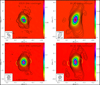 |
Fig. 1 ALMA continuum emission maps of M 2-9 at 232.9 GHz (left) and 95.4 GHz (right). The top row displays the images after image restoration using the nominal beam size at each frequency (Sect. 3). The bottom row presents the images with a circular restoring beam of 0.″04 at both frequencies, allowing for an optimal comparison between the two. The level contours are (3σ)×1.5(i−1) Jy beam−1, i =1,2,3… The central cross marks the 3 mm continuum surface brightness peak at coordinates J2000 RA=17h05m37s.9668 and Dec=−10º08′32.″65 (J2000). The yellow arcs, centered at the small yellow cross, represent the broad-waist structure, plausibly a dust disk, detected at 1 mm but not at 3 mm. |
4.2 Spectral energy distribution: Free-free and dust continuum emission
The overall fit to the continuum fluxes (Table 1) derived from 1mm to 3 mm as a function of frequency yields Sν ∝ ν0.92±0.1 (Fig. 2-left), consistent with predominantly free-free emission from the compact ionized wind/core of M 2-9 with a secondary contribution from dust thermal emission, as discussed in Sect. 2.
The spectral energy distribution (SED) of M 2-9 from the near infrared (NIR) to the radio domain, including our ALMA continuum flux measurements, is shown in Fig. 2 (right). Comparing the ALMA fluxes with the majority of the mm continuum fluxes obtained with single-dish telescopes reveals flux losses of approximately 20% in our high-resolution interferometric measurements. This finding indicates that ALMA, in the extended configuration used in this work (with MRS∽0.″7−0.″8, Sect. 3), is filtering and losing the contributions from both the free-free emission originating from the extended ionized lobes, which results in a nearly flat continuum flux of ∽30 mJy (Kwok et al. 1985), and the dust emission from extended structures. These extended structures include the relatively cool dust present in the large-scale bipolar lobes (with temperatures ranging from ∽5–25 K up to ∽100 K, Sánchez Contreras et al. 1998; Smith & Gehrz 2005) as well as the dust in the inner ∽1–2″-sized (in radius) equatorial disk (Castro-Carrizo et al. 2017) and whose temperature remains unconstrained.
Besides the extended dust structures, the mid-IR images of M 2-9 reported by Smith & Gehrz (2005) revealed the presence of an unresolved central core, suggesting the existence of a compact dust component at the center. A fitting of the mid- IR photometry of this unresolved central core (red solid line in Fig. 2-right) indicates an approximate temperature of ~260 K. This finding was further supported by Lykou et al. (2011), who used mid-IR interferometry to confirm the presence of a compact disk with approximate dimensions of 37×46 mas at 13 µm. Unlike the emission from the extended dust structures mentioned in the previous paragraph, the emission from this compact disk is not expected to be affected by interferometric flux losses in our ALMA maps. Therefore, it is likely that the compact warm disk, which exhibits its peak emission in the mid-IR, is contributing to the total observed mm continuum flux. Moreover, it is plausible that this compact disk corresponds to the inner, warmer regions of the broad-waisted structure detected in our 1 mm continuum maps, as supported by the fact that the dimensions of the broadwaist are comparable to (although slightly larger than) the size of the disk observed in the mid-IR (Fig. 1).
Under the assumption that a fraction of the mm continuum flux observed with ALMA originates from the warm (~260 K) compact disk we can achieve a good fit of the mm continuum with a combination of a ~200–300 K dust contribution (with emissivity ranging from ~0.2–0.5) and a free-free component that varies as Sν ∝ ν0.89 (Fig. 2). The latter component accurately reproduces both the cm-wavelength continuum (exclusively from the ionized wind/core as reported by de la Fuente et al. 20225) and the residual mm-wavelength continuum obtained by subtracting the ~260 K dust emission from the total mm continuum flux observed with ALMA.
It is important to emphasise that the decomposition/fit described above is subject to uncertainties and should be considered as a rough estimate, its main purpose being to provide an approximate value for the purely free-free continuum flux at mm-wavelength to be compared with the predictions from the model of the central ionized region presented in Sect. 6.1.
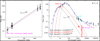 |
Fig. 2 Spectral energy distribution of M 2-9. Left: total (dust and free-free) mm continuum fluxes measured with ALMA in different SPWs (filled circles, Table 1). The global fit (Sν ∝ v0·92±0·1) is depicted with a solid line. The dashed line represents a fit to the free-free emission in the radio continuum, using the 4.9–43 GHz datasets from de la Fuente et al. (2022), which also reproduces our mm continuum fluxes after subtracting the contribution from a compact ~260 K dust component (shown in the right panel) – open squares. Right: SED of M 2-9 from the near-IR to the radio domain as in Sánchez Contreras et al. (2017) and including our ALMA mm continuum flux measurements (cyan). Radio continuum flux measurements at 4.9–43 GHz from the ionized wind/core as reported by de la Fuente et al. (2022) are indicated with pink circles. Mid-IR photometry of the compact, warm (~260 K) dust disk at the core of M 2-9 is shown with red triangles in the 8-20 µm range. Fits to the free- free and dust thermal emission are depicted, with the nearly flat continuum from the ionized bipolar lobes and the free-free emission from the ionized wind/core (Sv ∝ ν0·89) shown as a dotted-dashed and a dashed line, respectively. Several modified black-body components are also plotted, including a ~95 K component originating from dust located in the extended bipolar lobes, and filtered in our ALMA maps, (dotted line) and a ~260 K component arising from dust in a compact disk at the center of M 2-9 (red line). For completeness, a hot ~600 K dust component, which is necessary to explain the optical/NIR photometry, is also represented. The blue solid line represents the combined fits for the free-free and dust emission components. The red triangles at 1 mm and 3 mm represent the residual dust emission of M 2-9 after subtracting a Sv ∝ ν0.89 free-free emission component from the ionized wind/core. |
5 Line emission
We observed several mRRLs (including, H30α, He30α, H39α, and H55γ) in M 2-9 using ALMA. The He30α and H55γ lines are first detections, while H30α and H39α single-dish spectra were previously reported by Sánchez Contreras et al. (2017). Despite the high sensitivity of our ALMA data, the weak H51ϵ and H63δ lines were undetected. We have also mapped two rotational transitions of carbon monoxide (12CO 2–1 and 13CO 1–0). While the 12CO 2–1 emission has previously been mapped with NOEMA at a resolution of 0.″8×0.″4 (Castro-Carrizo et al. 2012), there are no known reports of 13CO 1–0 line maps.
5.1 Millimeter recombination lines
The observational results from our ALMA data of the H30α and H39α transitions, which are main targets of this study, are summarized in Figs. 3 and 4. The complete velocity-channel maps of these transitions are reported in Figs. A.2 and A.3. Additionally, we summarize our results for the He30α and H55γ transitions in Figs. A.4 and A.5. The line parameters derived from the source-integrated line profiles of the mRRLs detected are reported in Table 2.
Morphology and dimensions of the mRRL-emitting region. Consistent with expectations, the H30α and H39α emission originate from a compact region that shares similar shape and dimensions with the continuum emitting area at 1 and 3 mm, respectively. The integrated intensity maps of the H30α line do not exhibit any emission corresponding to the broad-waist component that is observed in the 1 mm continuum maps at a similar frequency and angular resolution (Fig. 1). Since H30α exclusively traces free-free emission, the lack of detection of the broad-waist component in the H30α line supports our earlier conclusion that this component is primarily associated with dust emission in the equatorial region.
After deconvolution with the beam, the H30α line emission in our ALMA maps (at a 3σ level) extends along the axis to a radial distance of ~0.″07 (∽45 au at d=650 pc) from the center. In the perpendicular direction, it extends to ~0.″045 (~30 au). As expected, the optically thicker H39α line, extends up to slightly larger radial distances of ~0.″11 (~70 au) and ~0.″063 (~40 au) along the axis and equator, respectively (after beam deconvolution and at a 3σ level). The major-to-minor axis ratio is larger for the H39α line (~l.75) compared to H30α (~l.5). This is well aligned with a previously reported size-to-frequency dependency that differs along the axis and along the equator (Lim & Kwok 2003).
Kinematics. For both the H30α and H39α transitions, we observe a clear velocity gradient along the axis of the nebula. The emission shows a redshift in the North (receding) lobe and a blueshift in the South (approaching) lobe indicating a global expansion along the axis. The position-velocity (PV) diagrams shown in Fig. 4 offer additional insights into the velocity structure of the ionized bipolar wind in M 2-9. The H30α emission exhibits a distinct S-shape pattern in the axial PV diagram, indicating an abrupt increase of the range of the line-of-sight velocities in two diametrically opposed, compact regions located at offsets δy~±0.″02 along the axis. While the S-shape is less pronounced in the H39α transition, a similar behavior is observed. As shown in Sect. 6.1, our model-based analysis of the mRRL emission maps suggests velocities of ~70–90 km s−1 in these regions, which are well described by high-density, high-velocity shell-like structures. We refer to these compact regions as the high-velocity spots/shells (HVSs).
The average velocity gradient observed in the inner regions of the ionized wind is ∇v~1150 km s−1 arcsec−1~l.8 km s−1 au−1, which results in extremely short kinematical ages of less than one year (after deprojection considering i~l7°, Sect. 2). This implies that observable changes in the profile of the mRRLs can occur in less than a year if there are variations on a similar timescale in the mass-loss rate, structure, or kinematics of the ionized wind.
The PV diagrams along the equator of both H30α and H39α reveal the presence of a subtle velocity gradient perpendicular to the lobes. Specifically, the east side of the equator (δx>0″) exhibits blue-shifted velocities, while the west side (δx<0″) shows red-shifted velocities. This is most evident in the velocity (first moment) maps of the lines, where the isovelocity contours are inclined rather than running parallel to the equatorial direction (Fig. 3). This behavior suggests rotation (counterclockwise) of the ionized bipolar wind.
Line profiles. Both the H30α and H39α transitions show a nearly Gaussian source-integrated profile. The H30α line has a peak of emission at VLSR=73±0.4 km s−1 and full width at half maximum of FWHM~44.8±0.9 km s−1. The weaker H39α transition is centered at a slightly larger velocity VLSR=75.1 ±0.7 km s−1 and is somewhat broader, with a FWHM~54.0± 1.7 km s−1. For both transitions, weak emission wings are observed with FWZI~130 km s−1.
The comparison of the source-integrated line profiles as observed with ALMA and with the IRAM-30 m single-dish reveals apparent differences (Fig. 3). The most significant changes are observed in the H30α line, which exhibits a notable increase in brightness (by a factor of ~2.2 in line flux and ~1.6 in line peak intensity) and broadening of the profile, with the FWHM increasing by ~11 km s−1. For H39α, we do not confirm an increase in brightness, but the line profile is broader by ~ 14 km s−1 in FWHM. In both transitions, the presence of broad wings in the ALMA observations that were not detected in the previous IRAM-30 m data suggests that these extended features have recently emerged or become more prominent. These differences are unlikely due to mispointing or flux calibration uncertainties (within nominal values of ~2–3″ and ~20% for the IRAM-30 m data, Sánchez Contreras et al. 2017), as these factors do not account for the observed variation in profile width.
The observed temporal variations of the mRRL profiles indicate changes in the gas dynamics or physical conditions of the central ionized wind of M 2-9 occurring over short timescales of ~2 yr or less. This is not surprising given the short kinematic age estimated for the inner regions of the mRRL-emitting regions. Changes in the profiles of mRRLs on short (~2-25 yearlong) timescales have been reported in the pPNe CRL 618 (Sánchez Contreras et al. 2017) and the post-supergiant candidate MWC 922 (Sánchez Contreras et al. 2019).
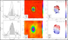 |
Fig. 3 Summary of ALMA data of the H30α (top) and H39α (bottom) lines (see also Figs. A.2 and A.3). Left: integrated line spectrum obtained with ALMA (black lines) and with the IRAM-30 m antenna (gray histogram, CSC17). Middle: line emission maps integrated over the line profile (LSR velocity range [11:143] km s−1). The level contours are (3σ)×1.5(i−1) Jy beam−1, i =1,2,3… Right: first moment map. Contours going from VLSR=45 to 115 km s−1 by 5 km s−1. The color bars indicate the VLSR-colour relationship. |
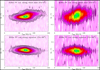 |
Fig. 4 Position velocity cuts of the H30α (left) and H39α (right) lines through the center along the wind axis (left, PA=0°) and the perpendicular direction (right). Levels are 2.5×(1.3)(i−1) for H30α and 1.5×(1.3)(i−1) for H39α with i =1,2,3… |
Line parameters from Gaussian fitting to the source-integrated profiles of the mRRLs in this study.
5.2 CO lines
While our study primarily focuses on mRRLs, we simultaneously mapped with ALMA the 12CO 2–1 and 13CO 1–0 lines (Table 1). As discussed in Sect. 1, CO (sub)mm-wavelength emission traces two off-centered, expanding equatorial rings (with radii of ~1.″1 and ~3–4″) that have been previously mapped with the NOEMA and ALMA interferometers and extensively studied by Castro-Carrizo et al. (2012) and Castro-Carrizo et al. (2017), respectively. As a result, do not study the CO emission from the rings in this work.
Our only focus will be on a newly discovered absorption component detected towards the continuum source both in the 12CO and 13CO observed transitions (Figs. 5 and A.6). We observe a narrow (FWHM~3 km s−1) CO absorption feature below the continuum level near the center of the nebula at velocity VLSR~80–81 km s−1, i.e., redshifted relative to the centroid of the mRRLs. The absorption indicates that the excitation temperature in the CO absorbing layers is lower than that of the continuum background source, which corresponds to the compact collimated ionized wind. Interestingly, the CO absorption feature is not centered at the nebula’s center but is slightly offset by δy~0.″012 towards the north. Given that the north lobe is moving away from the observer (with an inclination i~l7°), this offset suggests that the structure responsible for the absorption is likely an equatorial torus or disk surrounding the collimated ionized wind and positioned perpendicular to the lobes. In this configuration, the front side of the disk partially blocks the emission from the base of the receding north lobe, resulting in the observed CO absorption.
The observed redshift rules out that the absorption is produced neither in the arcsecond-scale central rings nor in the hourglass-shaped structure emerging from them reported by (Castro-Carrizo et al. 2017), since all these structures are in expansion and would necessarily produce a blue absorption given their spatio-kinematic structure, which is very well characterized in the mentioned previous works. The redshift of the CO absorption feature by ~6.2 km s−1 (deprojected velocity adopting i =17°) with respect to the velocity centroid of the mRRLs (Table 2) , likely signifies gas infall movements from the disk toward the central source. This is further discussed in Sect. 6.2.
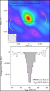 |
Fig. 5 Compact 12CO (J=2−1) absorption feature observed toward the central regions of M 2-9. Top: integrated intensity map of the CO absorption in the velocity range VLSR=[77.25:83.6] km s−1. Dashed and solid lines are used for negative and positive contours, respectively. Level spacing is 2σ to −13σ by −2σ (σ=4 mJy/beam). The yellow arcs represent the outer boundary of the broad-waist structure, plausibly a compact dust disk, observed in the 1 mm continuum maps. Bottom: line profile integrated over the area where CO absorption is observed. |
6 Analysis
6.1 NLTE radiative transfer modeling of mRRL and free-free continuum emission
We have modelled the free-free continuum and mRRL emission in M 2-9 using the NLTE three-dimensional radiative transfer code Co3RaL (Code for 3D Computing Continuum and Recombination Lines). The code and our modeling approach are described in detail in Appendix B.
Our modeling of the compact ionized wind in M 2-9 with Co3RaL began by employing the identical physical model utilized by CSC17 (see their Table 4). This model has been previously shown to accurately replicate the single-dish free-free continuum flux measurements and mRRL profiles observed in 2015 by these authors. As expected, this original model (which generates synthetic single-dish data closely resembling those from MORELI6) fails to capture some of the characteristics of the ionized wind now revealed by our ALMA ~0.″03–0.″06- resolution maps (Fig. D.1).
To obtain an improved model that fits these new details, we progressively adjusted the parameters of the input model (exploring a wide range of physical conditions and over ~300 models) until a reasonable match was achieved between the model predictions and the data. The ALMA-based improved M 2-9 model presented here, contrary to the one in Sánchez Contreras et al. (2017), has not been run under the LTE approximation but in NLTE. This is because the new ALMA data show a frequency dependence of the integrated flux of the Hnα lines steeper than observed in 2015 with the IRAM-30 m radiotelescope and deviating from the expectations in LTE. The best-fit model parameters are summarized in Table 3 and Fig. 6, and the predicted free-free continuum and mRRL emission maps are shown in Figs. 7–9. Throughout the modeling process, we kept the number of model parameters as low as possible, aiming at simplicity.
With regard to the wind’s structure, although the cylindrical geometry remains a reasonable approximation, the new observations necessitate two significant changes: (i) a much narrower bipolar structure (particularly an outer radius value of Rout~40 au), to reproduce the elongation of the maps and avoid generating excessively extended emission in the transverse direction compared to the data, and (ii) a narrow waist at the base of the wind (Req~8 au) to prevent excessive emission from the central regions. Additionally, we introduced a C-shaped curvature to the bipolar outflow to closely match the analogous shape observed in the 3mm continuum maps. While this paper does not address centimeter-wavelength properties of the free-free continuum, which originates well beyond the mm-wavelength emission’s spatial range, we observed that gradually widening the wind beyond axial distances of 15– 20 au (i.e. emulating a trumpet-like or hyperbolic horn shape) yields also a better match of the cm-continuum fluxes and best reproduces the faint, extended emission observed in the 3 mm continuum maps beyond δy~0.″12. Various inclinations for the line-of-sight axis of the wind around i =17° were examined, with the most successful models having an inclination of i =12°.
Regarding the wind’s density structure, a notable difference compared to the previous model is the necessity to include well- defined regions with different density profiles. These regions are defined as the nucleus (I), the inner wind (II), the HVSs (III), and the outer wind (IV) – see Fig. 6. Specifically, to reproduce the relatively bright emission from the HVSs it becomes necessary to introduce a relatively dense, shell-like structure at axial distances of ~15–30 au from the center within the wind. Without these dense shells (i.e. with a unique, smooth density power-law) is not possible to reproduce the S-shape of the axial positionvelocity diagrams observed for H30α and H39α. Immediately below and above the HVSs are the inner and outer winds, respectively. The density in the outer wind primarily determines the cm-continuum flux and the surface brightness of the 3mm continuum immediately beyond the HVSs. Meanwhile, the density of the inner wind is constrained by the 1mm continuum maps and the line-to-wings intensity ratio of the mRRLs. The maximum electron density in the central regions interior to the HVSs is constrained to ne<3×108 cm−3 by the full width of the H30α line: higher electron densities would produce excessively broad emission wings from the core (offset δy=0″) due to electron pressure broadening (see also model caveats in Appendix E). Since the density of the inner wind cannot be larger than this maximum ne value, a nuclear compact region (assumed spherical and with constant ne=2.5× 108 cm−3, for simplicity) is then necessary to reproduce the mm continuum flux level, which otherwise would fall below the observed values.
To simplify, we maintain a constant value for the electron temperature throughout the various regions of the wind. It is worth noting that while we cannot entirely rule out the possibility of temperature fluctuations within the wind, this factor alone cannot provide a satisfactory fit of the observed brightness distribution in the mRRL emission maps7. The value deduced Te ∽15 000 K, which should be taken as a representative average value within the ionized wind regions under study, is higher than than derived by CSC17 based on observations obtained 2 years earlier (Te∽7500 K). While there are uncertainties of up to ΔTe∽15–20%, the observed increase in the average electron temperature in the ionized wind might indeed reflect real variations in the wind’s properties over time, for example, an increase of the electron temperature may reflect an increase of collisional ionization as a result of recent propagation/development of shocks.
In terms of wind kinematics, the distinctive S-shape observed in the position-velocity diagrams along the axis of the mRRLs can only be explained by incorporating a steep velocity rise at the HVSs, which has been approximated by a step function. This step function represents a low velocity of ∽10 km s−1 within distances less than ∽15 au; beyond this point, i.e. within the HVSs, the velocity rises from ∽70 to ∽90 km s−1. Beyond the HVSs, in the outer wind, the velocity remains unconstrained as the line emission from these tenuous regions is below our detection limit. Within the HVSs, we explored alternative velocity functions that varied in steepness (including constant velocity), but these produced a poorer match to the data. Our best-fit model also includes rotation, which is needed to reproduce the observed velocity gradient perpendicular to the lobes (Sect. 5.1). In Fig. A.7 we show a model with no rotation for comparison. Since the angular resolution of the data does not allow us to distinguish between Keplerian or momentum conservation velocity profiles, we have used a constant rotation velocity of 7 km s−1 for simplicity. This value (at a representative radius of Req=8 au) implies a lower limit to the central mass of ≳0.4 M⊙.
The total ionized mass within the model region that produces the observed (sub)mm-to-cm free-free continuum and mRRL emission is Mion∽4×10⁻⁶ M⊙, similar to that obtained by CSC17. Considering the mean kinematical age of the wind, <tkin>∽6 yr, the average mass-loss rate implied from the model is Ṁ∽7× 10⁻⁷ M⊙ yr−1, which is also in good agreement with the value obtained by CSC17. This agreement is expected because, as discussed in CSC17, the mass/mass-loss rate is almost exclusively constrained by the flux of the free-free continuum, which has not shown discernible variations considering flux uncertainties (∽5–10% in our ALMA data and ∽20–30% in the IRAM-30 m data analyzed by CSC17). The determination of the mass/mass-loss rate is subject to some uncertainty due to factors such as the uncertain distance to the source, the simplified model used for the structure and kinematics of the ionized wind, and the moderate range of acceptable values for different model parameters. This likely results in a mass/mass-loss rate uncertainty of a factor ≲2–3. We caution that given the relatively complex structure and density stratification in the ionized central regions of M 2-9, interpreting the meaning of the mass-loss rate is not straightforward (see Sect. 7.2). The total scalar momentum, kinetic energy, and the average mechanical luminosity of the ionized wind have been computed and are given in Table 3. Model caveats and other final modeling remarks are discussed in Appendix E.
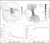 |
Fig. 6 Schematic view of the geometry and main parameters of our model of the ionized core of M 2-9 (Sect. 6.1 and Table 3). Top-left: 3D view indicating the four major structural components in our model, namely: nucleus (I), inner wind (II), high-velocity spots/shells (HVS, III), outer wind (IV). Colour scale represents density as indicated in the right wedge; arrows represent the velocity field (colour indicate blue or red Doppler shift with respect to the line of sight). The line of sight runs along the z-axis. Top-right: 2D view through the x=0 offset. Bottom panels show the radial distribution of the electron density (left) and radial expansion velocity modulus (right) adopted in our model. Vertical dashed lines indicate the boundaries of regions I-IV. |
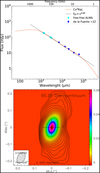 |
Fig. 7 Free-free continuum model predictions. Top: synthetic SED (red) along with empirical values of, and fit to, the mm-to-cm continuum flux as in Fig. 2-right. Bottom: synthetic 3 mm continuum map as in Fig. 1 top-right. |
6.2 CO absorption and 1 mm continuum: Evidence of a compact equatorial disk
In this section, we provide compelling evidence from our ALMA data supporting the existence of an equatorial disk composed of gas and dust surrounding the collimated ionized wind emerging from M 2-9 and oriented perpendicular to the lobes. This equatorial disk is probably the counterpart of the compact (∽37×46 mas) flattened dust structure observed along the equatorial plane of the nebula using VLTI/MIDI at 8–13 µm (Lykou et al. 2011).
First, as shown in Fig. 5 and briefly discussed in Sect. 5.2, the structure responsible for the CO absorption observed against the compact continuum source at the center of M 2-9 is likely an equatorial torus or disk surrounding the collimated ionized wind and positioned perpendicular to the lobes. In this configuration, the front side of the disk partially blocks the emission from the base of the receding north lobe, resulting in the observed CO absorption. Furthermore, differences in the brightness distribution of the continuum at 1 and 3 mm can also be attributed to the presence of an equatorial dust disk, which is expected to be the counterpart of the gas disk inferred from the CO absorption. In particular, at 1 mm, where dust-related effects are more prominent due to higher dust opacity and a larger contribution of dust thermal emission to the total emission (Fig. 2), the lower brightness of the northern lobe compared to the southern lobe can be partially explained by absorption of the free-free continuum from the collimated ionized wind that is behind the front side of the disk.
Additionally, the broad-waisted structure observed in the 1 mm continuum map (but absent at 3 mm and in the H30α maps) can be attributed to dust thermal emission from regions outside the narrower background continuum source, indicative of the presence of a dusty disk surrounding the ionized wind. Indeed, in contrast to the expected behavior for free-free continuum emission, we observe that the size of the waist is larger at 1 mm (reaching a maximum radius, at 3σ level, of ~0.″09 at 232.9 GHz – Fig. 1). However, in ionization-bounded or density-bounded H II regions, the free-free continuum emission decreases with increasing frequency or remains constant, as it is indeed observed in the mm-to-cm continuum maps of M 2-9 in the axial direction and at lower frequencies in both the equatorial and axial directions (Lim & Kwok 2003; de la Fuente et al. 2022). Therefore, the larger waist observed at higher frequencies is consistent with the contribution of dust thermal emission from the disk.
In the following, we attempt to establish some constraints on the physical conditions, including temperature and CO line opacity, as well as the dimensions (radius and vertical thickness) of the disk and its kinematics using the information contained in the CO absorption profile.
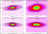 |
Fig. 9 Model position velocity cuts through the center of along the wind axis (left, PA=0°) and the perpendicular direction (right) as in Fig. 4. |
6.2.1 Physical conditions of the disk
As shown in detail, for example, by Sánchez Contreras et al. (2022) in their analysis of the compact NaCl absorption feature observed at the central rotating disk of the post-AGB nebula OH 231.8+4.2, the presence of absorption enables constraining the excitation temperature and opacity of the absorption line observed. This is done by comparing the brightness temperature of the absorption line (after continuum subtraction),  , the brightness temperature outside the continuum source,
  , and the continuum brightness peak in the same spectral window as the line is observed, Tc . Taking into account the values of the absorption and the upper limit to the emission measured in the CO maps of M 2-9 along with the continuum peak in the same spectral window8 (
 , and Tc~2350K), we deduce Tex≲330 K and τ~0.16. This value of the CO line opacity and Tex imply a CO column density of NCO≲6×1017 cm−2, for a line width of ~3 km s−1 (in this calculation we used the online version of the NLTE line radiative transfer code RADEX9 by van der Tak et al. 2007). Adopting a CO-to-H2 relative abundance of XCO=2×10⁻⁴, which is typical of O-rich sources (e.g. Ramos-Medina et al. 2018), we derive a total column density of
  cm−2 across the absorbing layers (along the line of sight) of the disk. However, this value represents a lower limit for the column density because the CO abundance used in the calculation is probably significantly overestimated due to strong photodissociation caused by intense ionizing radiation or shocks.
The outer radius of the disk can be estimated by considering the angular size of the broad-waist observed in the 232.9 GHz continuum map. From this analysis, an approximate value of Rout~0.″075 (beam-deconvolved; equivalent to ~50 au at a distance of 650 pc) is obtained, as discussed earlier in this section. This relatively large radius, along with the likely binary orbital separation of ≳15 au (Lykou et al. 2011; Castro-Carrizo et al. 2012; Sánchez Contreras et al. 2017), suggests the disk is most likely circumbinary rather than an accretion disk, which typically has a size comparable to or slightly larger than the radius of the accreting compact object. A lower limit to the disk radius can also be obtained from the offset to the north where the CO absorption is observed (rabs~0.″012~8 au). This lower limit arises from geometric considerations, as the CO absorption corresponds to the radius within the disk where the column density reaches its maximum, which is not expected to occur at the very edge of the disk. Assuming a line-of-sight inclination of i =12–17° for the disk equator, we can estimate a lower limit of R out≳27–38 au.
Based on the disk’s dimensions and the lower limit to the derived column density, we estimate the total mass to be Mdisk>2×10⁻⁶ M⊙. Additionally, the disk could be larger than what is seen in our ALMA maps, as the emission is probably limited by sensitivity, which would result in an even larger value for the disk gas mass.
The radius and the temperature of the equatorial disk in M 2-9 are similar to those of the circumbinary disk recently discovered at the center of OH 231.8+4.2, a well-known massive bipolar outflow associated with an AGB+main-sequence binary system (with a radius of ~40 au and temperature ~450 K, Sánchez Contreras et al. 2022). Assuming the average density of both disks is similar,  cm−3, we estimate the line-of- sight path length for CO absorption to be
  . The lower limit arises from the upper limit to the CO/H2 fractional abundance linked to a possibly enhanced CO photodissociation. This implies a vertical thickness of the M 2-9 disk, after deprojection, of h>0.6 au, resulting in an aspect ratio h/r>0.01 (or h/r>>0.01 if strong CO photodissociation).
6.2.2 Disk kinematics
The (deprojected) redshift of the CO absorption feature by ~6.2 km s−1 with respect to the systemic velocity of the background collimated ionized wind can be plausibly explained by gas infall from the disk toward the central region. Gas infall motions from the inner regions of circumbinary disks, formed e.g. in Wind Roche Lobe OverFlow (WRLOF) binary systems, is theoretically expected (e.g. Mastrodemos & Morris 1999; Mohamed & Podsiadlowski 2007; Chen et al. 2017) and has indeed been observed in a number of post-AGB objects with interacting binaries (e.g. R Aqr, Bujarrabal et al. 2021). An infall velocity of ~6.2 km s−1 observed at an average radial distance of rabs~27–38 au from the center (Sect. 6.2.1) would imply a central mass of ~0.7 M⊙, assuming that the gas started falling with (near) zero velocity from a point much far beyond the observed infall radius. This represents a lower limit for the central system’s mass since the closer we assume the fall started, the larger the estimated mass of the central system becomes. If we consider that the gas began falling in from the radius of the broad-waisted structure observed in the 1 mm continuum maps (~50 au) then the central mass would be ~2.0 M⊙. This should be regarded as an upper limit for two reasons. First, the radius of the disk in our maps might only represent a lower limit to the actual disk outer radius, which could extend beyond our sensitivity limit. Second, the infall velocity may be smaller than ~6.2 km s−1 if the centroid of the mRRLs is slightly blue-shifted relative to the systemic velocity of the source (as suggested by our model, Sect. 6.1 and Table 3). The mass range derived from these crude estimates is consistent with the previous assessments of the central binary’s mass by Castro-Carrizo et al. (2012), who proposed a low-mass companion of m2≲0.1–0.2 M⊙ orbiting around a m1∽0.5–1 M⊙mass-losing star.
In principle, rotation of the disk could also produce a red- shifted CO absorption feature if (and only if) the center of rotation and the center of the ionized region do not coincide, i.e., if both are off-centered. Only then will the rotational velocity have a non-zero component in the line of sight direction. In the context of a circumbinary disk, where the disk rotates around the center of mass of the system rather than around one of the binary components, the offset of the disk relative to the centroid of the ionized wind is expected. However, to observe a significant line-of-sight rotational velocity it is essential that the separation between the disk’s centroid and the ionized wind (denoted as rdw ) and the radial distance where most of the absorption occurs (denoted as rabs) are comparable. Our data allows us to estimate rdw to be around ∽0.″007∽5 au (Sect. 4.1) and rabs to be ∽38–27 au (Sect. 6.2.1). Therefore, to achieve a line-of-sight rotational velocity of ∽6.2 km s−1, the actual rotational velocity at ∽27–38 au should be  (from basic geometric calculations). Such a high velocity would imply an unreasonably massive central object, exceeding 30 M⊙.
7 Discussion
Both the nature of the central binary system residing in the core of M 2-9 and which of the stars is launching and ionizing the bipolar wind observed in our mm continuum and mRRL emission maps are two fundamental unknowns. In this section we analyze and discuss some of the results of our work with the aim of making progress in this regard.
7.1 Ionizing central source
As is well known (e.g. Condon & Ransom 2016), the number of Lyman continuum photons emitted per second (NLyC) needed to reproduce the emission from the ionized wind at the core of M 2-9 can be computed using the measured value of the free-free continuum flux (Sν) at a given frequency (ν) as:
 (1)
(1)
For an electron temperature of Te∽15 000 K (Sect. 6.1) and a free-free continuum of 102.80 mJy at 95.3 GHz (after subtracting the 260 K dust emission component from the total continuum fluxes in Table 1 – see also Fig. 2), we calculate a Lyman continuum photon rate of logNLyC∽43.8 s−1. This value has been compared with the Lyman continuum output rate from the grid of model atmospheres of early B-type stars by Lanz & Hubeny (2007) to investigate the central ionizing source. We find that a star with an effective temperature of around Teff∽25 kK (with R★∽1.3R⊙, adopting L★∽600 L⊙ at 650pc, and with a surface gravity log g[cgs]∽4, adopting a stellar mass of ∽0.5 M⊙, Sánchez Contreras et al. 2017) can account for the observed ionization. A similar effective temperature for the central ionizing source (early B-type or late O-type) was obtained by Calvet & Cohen (1978) from analogous considerations (and using continuum flux measurements at cm-wavelengths) but also independently by Allen & Swings (1972) and Swings & Andrillat (1979) from the analysis of the optical line emission spectra. This result implies that there is not need to invoke the presence of a hotter companion star to explain the observed nebular ionization in M 2-9.
If, as previously speculated, a white dwarf (WD) companion exists at the core of M 2-9 and is responsible for the observed nebular ionization, we can establish a lower limit to its effective temperature. By comparing the value of NLyC calculated from the mm continuum flux with the Lyman continuum output rate for WD stars expected from model atmosphere models by, e.g., Welsh et al. (2013), we find that the effective temperature of the WD must be larger than 50 000 K, implying a spectral type O 5 or earlier.
The luminosity and mass of the progenitor star of M 2-9 remain uncertain due to the lack of precise distance measurements (Sect. 1). At a distance of d=650 pc, adopted in this study, the luminosity of M 2-9 is below the expected value of ∽2500 Lø for the least massive stars (around 0.8 M⊙) that are expected to evolve off the main sequence within a Hubble time (Miller Bertolami 2016). A possible explanation for the low luminosity of the central star of M 2-9 is that it could be a post Red Giant Branch (post-RGB) object, meaning that it has prematurely left the RGB phase of stellar evolution. Recent studies have highlighted the existence of post-RGB stars with many characteristics similar to post-AGB objects, and it has been speculated that their peculiar evolution, deviating from standard models, may be influenced by strong interactions with close binary companions (Oudmaijer et al. 2022; Kamath et al. 2016; Hrivnak et al. 2020; Olofsson et al. 2019).
7.2 Implications of the mass-loss rate
The average mass-loss rate of the ionized bipolar wind at the core of M2-9 is deduced to be of Ṁw~10−7 M⊙ yr−1 (Sect. 6.1). Interpreting the meaning of the mass-loss rate is not straightforward when we are uncertain about which of the stars is responsible for launching the wind.
If the ionized wind emerges from the mass-losing star, then, the measured mass-loss rate of the present-day wind is significantly lower than the rates observed ∽1300 and ∽900 years ago, ~10−5 M⊙ yr−1, which were responsible for forming the large- scale nebula, including the massive CO equatorial rings (Sect. 1). In this scenario, the substantial reduction in the mass-loss rate with respect to previous epochs can be interpreted as evidence that the primary star has transitioned to a post-AGB or postRGB phase. Alternatively, the star could currently be in the AGB phase with a mass-loss rate of ṀAGB≈10−7 M⊙ yr−1, which is more in line with what is expected for a low-mass progenitor star, but the ejection of the large-scale nebula, including the CO rings, could have occurred at two specific moments with “abnormally” high rates.
If the ionized wind does not directly originate from the masslosing primary star but, instead, from its companion after mass transfer through disc-mediated accretion, it is expected that this wind would interact with the slow wind of the donor star. Such an interaction would give rise to a complex bipolar structure characterized by intricate density and velocity patterns, featuring multiple shock formations and a dense equatorial region as shown by analytical studies (e.g. Soker & Rappaport 2000; Livio & Soker 2001) and numerical simulations (García-Arredondo & Frank 2004). According to these investigations, if this scenario applies to M 2-9, the region responsible for emitting mRRLs would encompass the ionized portion of this complex structure10, including both the primary’s slow wind and the companion’s fast wind, both of which would exhibit significant structural and velocity alterations due to their interaction. In this context, the mass-loss rate estimated in our study is likely to fall between the mass-loss rates of the mass-losing star and that of the companion.
7.3 Wind structure and kinematics
Our ALMA observations show the presence of a collimated, ionized wind emanating from the center of M 2-9. As observed at mm-wavelengths, this narrow-waisted wind extends along the nebular axis direction up to radial distances of ~75 au and ~40 au in the perpendicular direction. Based on radio-continuum emission maps, the ionized wind extends up to least 230 au along the axis (Lim & Kwok 2003; de la Fuente et al. 2022), resulting in an aspect ratio of >4.5. This wind displays high-velocity motions, reaching speeds of ~80 km s−1, thereby categorizing it as a jet. One of the significant findings from our data and modeling is the presence of a non-uniform density structure within the jet: we find alternating regions with noticeable density variations, characterized by regions of high density and areas of low density. This density pattern may reflect the presence of shock- compressed regions and/or fluctuations in the mass-loss rate on short timescales.
The jet, as seen in the 3 mm continuum emission maps (Fig. 1), displays a distinctive C-shaped curvature, consistent with that observed in the JVLA 7 mm continuum emission maps ~11 years earlier (de la Fuente et al. 2022). As suggested by de la Fuente et al. (2022), evoking the old model by Livio & Soker (2001), the mirror curvature of the jet could be caused by the influence of the dense primary star’s wind on a jet hypothetically launched by the companion. We believe that the presence of poloidal magnetic fields could also be considered as an alternative explanation, potentially exerting a bending effect on the ionized wind along the field lines. By equating the magnetic and mechanical energy densities, we estimate that a magnetic field strength of ~50 mG could induce the observed curvature in the ionized jet, based on typical densities (~2×106 cm−3) and expansion velocities (~80 km s−1) in the outer regions of the jet (~30 au), where the curvature is observed. This estimate is in good agreement with existing, albeit limited, observations of magnetic fields in (post-)AGB envelopes at similar or even larger radial distances from the center (Blackman 2009; Vlemmings 2018).
In both cases, the orientation of the curvature depends on the relative position of the stars, which changes over time as the stars move in their orbit. Since the orientation of the curvature has remained unchanged since 2006, the star producing the bending effect is still situated on the same side relative to the star launching the jet. This observation is consistent with the small time lapse between the ALMA and JVLA observations, approximately one ninth of the orbital period (Porb~90 yr).
Our ALMA data have revealed the kinematics of the jet, showing a non-uniform velocity field with low-expansion velocities (~ 10 km s−1) at the center and maximum line-of-sight projected velocity widths of ~80 km s−1 at around ~ 15–30 au along the axis (HVSs). The abrupt change in velocity observed at/within the compact HVSs, relative to the center, can be interpreted in at least two ways. One possibility is that the wind acceleration occurs at these 15–30 au scales through some unknown mechanism, possibly a combination of line-radiation pressure and the magneto-centrifugal mechanism. Alternatively, HVSs may indicate a wider range of line-of-sight velocities arising from shocks within the ionized wind. Analytical bow-shock models (Hartigan et al. 1987) and numerical simulations (Dennis et al. 2008) predict substantial velocity spreads in compact, shocked regions, which are indeed observed in various pPNe (Dennis et al. 2008; Riera et al. 2006; Sahai et al. 2006). Internal shocks can arise due to variations in the wind expansion velocity, which aligns with the time-varying mRRL profiles of M 2-9 (Sect. 5.1). Shocks could also result from the interaction of the winds of the two central stars, assuming that both stars possess winds (e.g. Soker & Rappaport 2000; Livio & Soker 2001; García-Arredondo & Frank 2004).
8 Summary and conclusions
Using ALMA, we conducted a detailed mapping in bands 6 and 3 of the inner layers (within r~0.″2~130 au at d=650 pc) of the ionized core of M 2-9. The mm continuum and the H30α and H39α line emission were imaged with spatial resolutions reaching down to ~0.″03 and ~0.″06, respectively. Our data provide detailed evidence for the presence of a compact, bent jet expanding with velocities of up to ~80 km s−1 at the core of this remarkable object. Using the NLTE radiative transfer code Co3 RaL (Sect. 6.1 and Appendices B–E), we performed data modeling to derive valuable insights into the morphology, kinematics, and physical conditions of the jet. Our findings suggest a potential interaction between a tenuous companion-launched jet and the dense wind of the primary star. We can summarize our key findings as follows:
The region emitting mm continuum is elongated along the main symmetry axis of the nebula; it has dimensions of 0.″4×0.″13 (260×85 au at d=650 pc) at 3 mm and is slightly smaller at 1 mm due to the lower opacity of the free-free continuum at shorter wavelengths.
The spectral index of the continuum (~0.9) suggests predominantly free-free emission from an ionized wind, with a minor contribution from dust, which possibly originates from a warm compact disk.
The ionized wind is collimated and displays a C-shaped curvature at 3 mm, which is consistent with previous observations taken 11 yr earlier at 7 mm.
The 1 mm continuum map reveals a broad-waisted morphology oriented perpendicularly to the wind lobes, which is plausibly the counterpart of the compact ~260 K dust disk observed in the mid-IR.
CO and 13CO absorption features further support the presence of an equatorial disk with a radius of ~50 au (likely circumbinary), with gas infall toward the central source. Our analysis of the CO absorption feature suggests an excitation temperature of Tex≲330 K and a CO column density of NCO≳6×1O17 cm−2. A lower limit to the mass of the disk of >2×10⁻⁶ M⊙ is deduced.
Emission from H30α, H39α, He30α, and H55γ is detected, with line emission extending to radial distances of up to ~75 au along the direction of the nebular axis and ~40 au in the perpendicular direction.
Changes in the H30α and H39α line profiles over two years indicate variations in the wind’s kinematics and physical conditions. The wind has become faster during this time period.
Both the H30α and H39α transitions exhibit a distinct velocity gradient along the axis of the nebula, implying an overall expansion along the axis of the bipolar outflow.
Low expansion velocities of ~ 10 km s−1 are observed at the center. Rapid wind acceleration or shocks are suggested by peak velocities of ~70–90 km s−1 in two compact regions, situated at a radial distance of ~± 15–30 au along the axis (HVSs).
The ionized wind has a short kinematical age, including regions of less than a year old, explaining changes in the mRRL profiles on similar year-long timescales.
The emission maps of H30α, H39α, and He30α lines reveal a subtle velocity gradient perpendicular to the lobes that is suggestive of rotation (Vrot~7–10 km s−1).
Radiative transfer modeling indicates an average electron temperature of ~15 000 K and reveals a nonuniform density structure within the ionized jet, with electron densities ranging from ne≈106 to ≲108 cm−3. We deduced the mass and average mass-loss rate of the ionized wind, obtaining Mion~4×10⁻⁶ M⊙ and Ṁ≈10−7 M⊙ yr−1, respectively. These results potentially reflect a complex bipolar flow pattern resulting from the interaction of a tenuous companion- launched jet and the dense wind of the primary star.
The mass of the central system is uncertain, but it is likely in the range of 0.4 to 2 M⊙ based on the rotational and infall motions observed in the jet and the circumbinary disks, respectively, as described in this study.
The required number of Lyman continuum photons per second is consistent with a central star with an effective temperature of ~25 kK and a luminosity of ~600 L⊙, which is perhaps a post-RGB star. We do not find empirical evidence of fast (≳l000 km s−1) ejections indicative of a compact companion. While a WD companion is not ruled out, our findings do not provide empirical evidence for one.
The nature of the companion remains highly uncertain. Unravelling the nature of the central binary system of M 29 and the intricate interplay between the primary star and its companion are essential in order for us to understand the mechanisms governing the observed mass loss and wind dynamics in this system.
Data availability
Additional Figures A.1–A.6 can be found in Appendix A.
Acknowledgements
We would like to thank the referee, Joel Kastner, for his insightful comments and suggestions, which helped improve the clarity of this work. This paper makes use of the following ALMA data: ADS/JAO- .ALMA#2016.1.00161.S and ADS/JAO.ALMA#2017.1.00376.S. ALMA is a partnership of ESO (representing its member states), NSF (USA) and NINS (Japan), together with NRC (Canada), MOST and ASIAA (Taiwan), and KASI (Republic of Korea), in cooperation with the Republic of Chile. The Joint ALMA Observatory is operated by ESO, AUI/NRAO and NAOJ. This work is part of the I+D+i projects PID2019-105203GB-C22 and PID2019-105203GB-C21 funded by Spanish MCIN/AEI/10.13039/501100011033.
Appendix B The NLTE free-free continuum and mRRL radiative transfer code
Here, we provide a detailed description of our code used to model the free-free continuum and radio recombination line ALMA data presented in this work.
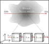 |
Fig. B.1 Division of a non homogeneous source into homogeneous cells. The physical conditions, density and temperature, can be considered constant within each cell. |
B.1 Numerical calculations of the solution of the radiative transfer equation
As is well known, the solution of the radiative transfer equation in a plane-parallel, homogeous, and isotropic medium can be expressed as:
 (B.1)
(B.1)
involving the frequency (ν), the optical depth (τν), the initial specific radiation at that frequency at the back surface of the source (Iν(0)), the specific intensity outgoing from the front surface of the source (Iν(τν)), and the source function (𝒮ν).
Astronomical sources are not completely homogeneous and the physical conditions vary from place to place. To address this, a common approach for computing the outgoing intensity of a realistically heterogeneous source is to partition it into small cells, each characterised by approximately constant physical conditions (refer to Fig. B.1). Once the source is subdivided into small cells with uniform temperature and density, Eq. (B.1) can be used to compute the outgoing intensity of each cell. As depicted in Fig. B.1, the outgoing intensity Iν,i−1 of cell i − 1 serves as the initial intensity Iν(0) for cell i, and similarly, the outgoing intensity of cell i is used as the initial intensity for cell i + 1, and so forth. The intensity of the pixel with coordinates (x,y), denoted Iν(x,y), is determined through successive computations of the radiative transfer equation solution (Eq. (B.1)) for cells along a single line of sight (i.e., along the z-axis). As a result, Iν(x, y) represents the resulting outgoing intensity of the cell positioned at the forefront of the source, closest to the observer.
B.2 Code for Computing Continuum and Radio-recombination Lines: Co RaL
The Code for Computing Continuum and Radio-recombination Lines (Co3RaL) is a C-based code designed to calculate the intensity of the free-free continuum and recombination line emission originating from an ionised nebula. It operates on user- defined geometrical shapes that can be specified analytically and relies on provided density, temperature, and velocity fields given by analytical functions. The outputs are ASCII tables containing information needed to generate continuum images, spectral energy distribution (SED) plots, spectral cubes, and spectral line profiles.
B.2.1 Definition of the geometry
The grid of cells considered by Co3RaL, within which the geometry of the emitting region is defined, is created in a coordinate system C. The coordinates of each cell are given within the intervals [−xmax, xmax], [−ymax, ymax], and [−zmax, zmax] for the x, y, and z axes, respectively. The x−y plane corresponds to the plane-of-the-sky, while the z−axis corresponds to the line-of- sight. Each interval is evenly divided into nx , ny , and nz cells along the respective axis. Co3RaL sweeps through the cells of the grid along the z-axis and calculates the outgoing intensity for each cell until it reaches the cell positioned at the forefront of the source.
The boundaries of the emitting region (i.e., the cells where the density and temperature are non-zero) are defined by an analytical function in a coordinate system C′ . In general, the coordinate system C′ is rotated with respect to the coordinate system C (see, for example, Fig. B.2). Consequently, the emitting region typically appears rotated relative to the C′ system. Co3RaL sweeps through the cells of the grid along the z-axis of the coordinate system C. When it reaches a cell with coordinates (x, y, z), it transforms the coordinates from C to C′ using the following rotation matrix:
![Mathematical equation: $\left[ {\matrix{ {{x^\prime }} \hfill \cr {{y^\prime }} \hfill \cr {{z^\prime }} \hfill \cr } } \right] = \left[ {\matrix{ {\cos (\phi )} & {\sin (\phi )} & 0 \cr { - \cos (\theta )\sin (\phi )} & {\cos (\theta )\cos (\phi )} & { - \sin (\theta )} \cr { - \sin (\theta )\sin (\phi )} & {\cos (\phi )\sin (\theta )} & {\cos (\theta )} \cr } } \right]\left[ {\matrix{ x \hfill \cr y \hfill \cr z \hfill \cr } } \right],$](/articles/aa/full_html/2024/12/aa51669-24/aa51669-24-eq13.png) (B.2)
(B.2)
where θ and ϕ are the inclination angle with respect to the plane of the sky and the position angle of the source, respectively. Once the coordinates of the cell are transformed into the coordinate system C′, Co3RaL checks whether the cell is within the emitting region. If the cell is within the emitting region, the radiative transfer is performed using Eq. (B.1). If the cell is outside the boundary of the emitting region, it is skipped, meaning it is assumed that the cell does not affect the intensity Iν, and the code moves to the next cell along the line-of-sight. The resulting intensity for each line-of-sight, Iν(x, y), is output using the coordinates of the coordinate system C. It is worth noting that, since the radiative transfer is performed along rays in the line-of-sight, the result of the calculations is sensitive to the inclination of the source but not to the position angle.
B.2.2 Definition of the physical parameters
The definition of the physical parameters is more straightforward in the rotated C′ system, where they are expressed as relatively simple analytical functions dependent on the primed coordinates: T (x′, y′, z′), n(x′, y′, z′), and ν(x′, y′, z′). However, as mentioned above, Co3RaL sweeps through the cells of the grid along the z-axis of the coordinate system C. Thus, for each cell within the emitting region, Co3RaL transforms the coordinates (x, y, z) to (x′, y′, z′) (using the rotation matrix in Eq. (B.2)), and then calculates the corresponding values of the physical parameters using the analytical functions defined in the C′ system. Subsequently, the outgoing intensity of the cell is calculated iteratively using Eq. (B.1) and the physical parameter values specific to that cell.
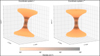 |
Fig. B.2 Geometry of the emitting H II region as seen in the coordinate system C (left) and coordinate system C′ (right). The source can be rotated in the C system, but by definition it is not rotated in the C′ system. |
B.2.3 Computation of the radio continuum
To compute the radio continuum emission, Co3RaL uses the following free-free emission coefficient (Rybicki & Lightman 1986):
 (B.3)
(B.3)
where ne and ni are the electron and ion densities, respectively, Z is the electric charge of the ions, Te is the electron temperature, h and k are the Planck and Boltzmann constants, ν is the frequency of the radiation, and g(ν, Te) is the Gaunt factor, which is the sum of the Gaunt factors for free-free and bound-free transitions, g(ν, Te) = gff + gbf.
Following Báez-Rubio et al. (2013), the Gaunt factor for free- free transitions is calculated in the following way:
 (B.4)
(B.4)
where K0(x) is the modified Bessel function of the second kind and
 (B.5)
(B.5)
 (B.6)
(B.6)
 (B.7)
(B.7)
 (B.8)
(B.8)
where ν0 is the hydrogen ionisation frequency with a numerical value of ν0=3.291×10¹⁵ Hz.
The modified Bessel function of the second kind, K0(x), is computed using the following approximation (Martin & Maass 2022):
 (B.9)
(B.9)
The Gaunt factor for bound-free transitions is calculated in the following way (Brussaard & van de Hulst 1962):
 (B.10)
 (B.11)
 (B.12)
where int(x) is the nearest integer value (rounded off value) of x. As pointed out by Báez-Rubio et al. (2013), the value of gn (ν) is taken as unity for all the considered frequencies, which yields results with an accuracy of ∼10 – 20%. However, it is worth noting that the Gaunt factors for bound-free transitions become significant only for frequencies ν≳104 GHz (see Fig.A.1 of Báez-Rubio et al. (2013)). Thus, this factor is negligible for RRLs.
Subsequently, the absorption coefficient, κν, is obtained using Kirchhoff’s law as
 (B.13)
where Bν(T) is the Planck function given by
 (B.14)
The optical depth,  that is used in Eq. (B.1) to compute the intensity of the continuum emission is thus computed as
 (B.15)
where dl is the physical size of the cell, given in CGS units.
B.2.4 Computation of the radio recombination lines in LTE conditions
Co3RaL computes the emission of RRLs in LTE and NLTE conditions. The emission of the lines in LTE conditions is computed using the following absorption emission coefficient (Wilson et al. 2009):
 (B.16)
where νul is the central rest frequency of the line, nu is the upper level electronic quantum number, and Vν is the Voigt profile of the line, obtained as a convolution of Gaussian and Lorentzian profiles. Using the notation of Kielkopf (1973), the expression of the convolution is given as follows:
 (B.17)
where βl and βg are the Lorentzian and Gaussian widths, defined as the half width at half maximum. Given that the calculation of this convolution needs to be done for every cell, it turns out to be computationally expensive. Therefore, Co3RaL uses the approximation to the convolution given by Kielkopf (1973):
 (B.18)
where I(βl , βg) is given as
 (B.19)
and the expression for U(x) is the following:
![Mathematical equation: $U(x) = (1 - \eta )G(x) + \eta L(x) + \eta (1 - \eta )E(x)[G(x) - L(x)].$](/articles/aa/full_html/2024/12/aa51669-24/aa51669-24-eq32.png) (B.20)
(B.20)
The factor a in Eq. (B.19) is defined as the ratio of the Lorentzian and Gaussian widths, a = βl/βg, and the form of the function f (a) depends on the value of a as follows:
 (B.21)
where
 (B.22)
and b0 = 0.47047, b1 = 0.61686, b2 = −0.16994, and b3 = 1.32554.
The functions G(x), L(x), and E(x) in Eq. (B.20) are defined as follows:
 (B.23)
 (B.24)
 (B.25)
The factor η in Eq. (B.20) is defined as follows:
 (B.26)
where
 (B.27)
![Mathematical equation: $\beta = {1 \over 2}{\beta _l}\left\{ {1 + \ln (2) + {{\left[ {{{(1 - \ln (2))}^2} + \left( {4.0\ln (2)/{a^2}} \right)} \right]}^{1/2}}} \right\},$](/articles/aa/full_html/2024/12/aa51669-24/aa51669-24-eq40.png) (B.28)
(B.28)
 (B.29)
and є=0.0990.
The Gaussian width of the line, βg, is calculated using the following expression (Mezger & Hoglund 1967):
 (B.30)
where mH is the mass of the hydrogen atom and νtuг is the turbulent velocity due to turbulent motions of the plasma. The expression of the Lorentzian width, βl, is taken from Table B.1 of Báez-Rubio et al. (2013).
Finally, the optical depth of the line,  , in LTE conditions is given as
 (B.31)
and the total optical depth,  , which is used in Eq. (B.1) to compute the intensity of the line plus continuum, is the sum of both optical depths:
 (B.32)
After performing the radiative transfer for the line plus continuum, the emission from the continuum is subtracted to obtain the emission from the line only.
B.2.5 Computation of the spontaneous emission Einstein coefficients
The relationship between the Einstein coefficient for spontaneous emission, Aul, and the thermalised absorption oscillator strength f (nl, nu), with nu > nl, is given by (Goldwire 1968):
 (B.33)
where α is the fine structure constant, Z is the atomic number, c is the speed of light, and RM is the Rydberg constant defined as
 (B.34)
with me being the mass of the electron and M denoting the total mass of the nucleus. Furthermore, R∞ is given by
 (B.35)
where e represents the elementary charge, ε0 is the permittivity of free space, and h stands for the Planck constant. The numerical value of R∞ is 109737.315685 cm−1.
The most straightforward way to calculate the oscillator strengths is using the following expression given by Kardashev (1959):
 (B.36)
where the parenthesis  is the binomial coefficient, F(a, b, c; z) is a hyper-geometric function and x is defined as
 (B.37)
Thus, by substituting Eq. (B.36) into Eq. (B.33), the Einstein coefficient for spontaneous emission can be calculated. This approach requires evaluating the hyper-geometric function in Eq. (B.36), which is not included in Co3 RaL. Therefore, the Einstein coefficients for spontaneous emission are calculated separately, and Co3RaL reads the values from a table.
B.2.6 Computation of the radio recombination lines in NLTE conditions
Non-local thermodynamic equilibrium conditions occur when the populations of the energy levels deviate from the Boltzmann distribution. The computation of RRL emission can be done by following the procedure introduced by Menzel (1937), in which departure coefficients bn relate the true population of a level, Nn , to the population under LTE conditions,  , by the relationship
  . Under this consideration, the Boltzmann equation becomes
 (B.38)
where gi (with i = u, l) are the statistical weights of the electronic levels, calculated as gi = ni2, and bi (with i = u, l) are the NLTE departure coefficients mentioned above. The value of the bi factors is always <1, since the Aul coefficient for the lower state is larger and the atom is smaller so collisions are less effective, bi→1 for LTE conditions Wilson et al. (2009). Using the expression of Eq. (B.38) in the expression for the absorption emission coefficient (Eq. (B.16)), the absorption emission coefficient under NLTE conditions can be written as
 (B.39)
Thus, the relation between the absorption coefficients under LTE conditions and NLTE conditions can be written in the following way:
 (B.40)
where the coefficient βul is defined as
 (B.41)
In general, the relationship between the emission and absorption coefficients for the line can be written as follows (Wilson et al. 2009):
 (B.42)
and using Eq. (B.38) we arrive to the following expression:
 (B.43)
Substituting Eq. (B.40) into this expression and using Kirchhoff’s law,  , it is possible to write the relation between the emission coefficients under LTE conditions and NLTE conditions in the following way:
 (B.44)
The expression for the source function under NLTE conditions is given by the following expression:
 (B.45)
which can be written as
 (B.46)
with
 (B.47)
Thus, the radiative transfer equation (Eq. (B.1)) for NLTE conditions becomes
 (B.48)
The NLTE departure coefficients, bi , are obtained from the tables provided by Storey & Hummer (1995) for Case B. These tables include values of NLTE departure coefficients for a range of temperatures from 500 to 30,000 K and densities from 102 to 1014 cm−3. Figure B.3 shows the values for nu = 40. As can be seen from Fig. B.3, the values are close to 1 for high electron densities and temperatures, and they have lower values for low densities and temperatures.
To obtain the value of the NLTE departure coefficients for any value of density and temperature, Co3RaL performs a two-dimensional linear interpolation. First, it interpolates the values between densities at the same temperature, and then it interpolates the values between two temperatures corresponding to the electron density in question. Figure B.4 shows a diagram of the procedure to find the value of the NLTE departure coefficient for any arbitrary electron density and temperature.
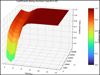 |
Fig. B.3 Storey & Hummer (1995) NLTE departure coefficients for the Case B and nu=40. |
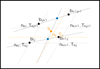 |
Fig. B.4 Diagram depicting the procedure to find the value of the NLTE departure coefficient for any arbitrary electron density and temperature. The gray dashed lines indicate the coordinates of the discrete values of density and temperature from the Storey & Hummer (1995) tables (shown as black dots). The orange dashed lines indicate the coordinates of an arbitrary value of electron density and temperature. The solid gray lines indicate interpolation between discrete coefficient values of different densities but the same temperature. The blue dots represent the points connecting the two linear interpolations at an arbitrary electron density. Finally, the orange dot corresponds to the value that Co3RaL uses for an arbitrary electron density and temperature. |
Various interpolation methods were tested to calculate the NLTE departure coefficients for different values of density and temperature. However, these methods did not result in significant differences in the outcomes. Therefore, the previously described method was chosen for its simplicity and efficiency.
B.3 Co3RaL general description and modeling approach
The Co3RaL code can consider any given 3D geometry for the ionized region. The geometry can be analytically described in Cartesian, spherical or cylindrical coordinates or, alternatively, it can be read from an input file where the coordinates of the model cells are provided. In addition to the geometry, the other major inputs for the model are: the electron density (ne), the electron temperature (Te), and the velocity field ( ). For simplicity, ne and Te are assumed to follow a power law of the type ∝rβ, where r is the radial distance to the central source and β is a real number positive or negative. Non-uniform distributions are accommodated by employing different laws, as necessary, across distinct layers within the ionized wind. The same approach can be applied to describe the velocity field, also allowing for various combinations of radial, axial, equatorial, and shear expansion, with equatorial rotation. The velocity modulus can be constant or increase/decrease as any given function of r. Latitude- and longitude-dependent variations can be incorporated for any of the input physical parameters. In addition to the gas macroscopic motions, thermal broadening as well as electron impact (pressure) broadening are included in the line profile function. In the present model of M 2-9 (Sect. 6.1), turbulence velocity dispersion is not considered as an additional form of line broadening since it is expected to be very small (σturb<2–3 km s−1) in the envelopes of AGB and post-AGB objects (e.g. Schöier et al. 2004; Bujarrabal et al. 2005; Decin et al. 2010) and, thus, negligible compared to other broadening terms.
Appendix C Comparison of Co3RaL with MORELI
In the pilot single-dish study of the emerging ionized regions of pPNe by CSC17, the free-free continuum and mRRLs emission was modelled using the radiative transfer code MORELI (Báez-Rubio et al. 2013). MORELI is a code previously employed in several studies of ionized regions, including works by Báez-Rubio et al. (2014); Sánchez Contreras et al. (2019); Martínez-Henares et al. (2023). Here, we present a comparative analysis between the predictions generated by our code, Co3RaL, and those produced by MORELI, utilizing identical input models. This comparison serves as a mutual benchmarking exercise of both codes. We separately run LTE and NLTE models for M 29 and CRL 618, respectively, pPNe that are both modelled by CSC17 using MORELI.
The two input models employed correspond to the configurations described for M2-9 and CRL 618 in Table 4 of CSC17, depicting in both cases a cylindrical outflow radially expanding, with the detailed geometry, physical structure, and kinematics of the cylindrical outflow being different for, and adapted to, each source. We refer to these preliminary models based on singledish data as CSC17’s models. As in CSC17, Co3RaL was run under the LTE approximation for M 2-9 and NLTE for CRL 618.
As shown in Fig. C.1, the predictions for the free-free continuum flux at (sub)mm-to-cm wavelengths, along with the mRRLs H30α and H39α, for Co3RaL and MORELI exhibit a high level of consistency. The continuum fluxes predicted by MORELI and Co3RaL are indeed almost identical, with differences falling below 1%–2% precision for both objects. Under LTE (M 2-9), the mRRLs line profiles are also identical. For NLTE (CRL 618), Co3RaL predicts slightly (10%–15%) higher peak intensities for both lines, resulting in a small difference in the best-fit electron temperature of TeCoRaL−TeMORELI≲700K (<4%) when derived using the two codes on the same data set, while keeping the rest of CSC17’s model parameters the same. Without access to the original MORELI source code, it is impossible to determine the exact reason for this small discrepancy. The discrepancy could be related to the various approximations and interpolations made when estimating the bn departure coefficients (available in the literature only for a discrete grid of electron density and temperature pairs), pressure broadening coefficients, integration of the Voigt profile, etc (see Appendix B for details).
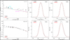 |
Fig. C.1 Comparison between the predictions by Co3RaL and MORELI for the input model of M 2-9 (LTE, top) and CRL 618 (NLTE, bottom) presented in CSC17 that were designed to reproduce the IRAM-30 m single-dish data reported by these authors – see Sect. C. Left) Synthetic free-free continuum emission spectrum predicted by Co3RaL (black solid line) and MORELI (red dashed line). Data points (circles), shown as a reference, are as in Fig. 1 for M2-9 and as in CSC17 for CRL 618. Middle and Right) Synthetic H30α and H39α 1d spectra (integrated over the emitting region) predicted by Co3RaL (solid black histogram) and MORELI (dashed red histogram). |
Appendix D Comparison of CSC17’s model for M 2-9 with new ALMA maps from this work
In Fig. D.1 we show synthetic ALMA-like cubes representing emission from 93 GHz free-free continuum and H30α and H39α lines, based on the model of M 2-9 derived from single-dish observations by CSC17. While this model accurately reproduces the free-free (mm-to-cm) continuum flux and the single-dish line profiles, the corresponding synthetic ALMA images reveal notable differences from the actual ALMA data (Figs. 1 and 4). These differences suggest the presence of a collimated wind or jet that is narrower than initially assumed and that exhibits a certain C-shaped curvature as well as a significant velocity gradient along its axis. In Sect. 6.1, we introduce an updated model that replicates these and other features observed in our ALMA datasets, which has a resolution of a few tens of milliarcsecond.
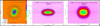 |
Fig. D.1 Synthetic ALMA-like cubes of the free-free continuum emission at 93 GHz (left) and the H30α and H39α lines (middle and right, respectively) obtained from the M2-9 model in CSC17 — see their Table 4 — to be compared with analogous datasets obtained with ALMA in Fig. 1 (top-right) and Fig. 4 (top panels). |
Appendix E Model caveats and final modeling remarks
It is important to emphasize that the relatively simple model presented in Sect. 6.1 is probably not unique and that more intricate geometries, kinematics, and density and temperature profiles (e.g., latitude-dependent) cannot be dismissed as possibilities. Although a comprehensive parameter space study has not been performed and is beyond the scope of this paper, we are confident that the bulk features deduced from the model– such as the presence of dense, high-velocity shell-like regions within a narrow-waisted bipolar (horn-like) wind– are robust and necessary to reproduce the main features inferred directly from the data. The model’s primary role is to reinforce these features and provide a more precise characterization of the physical properties in the wind. Below, we describe the uncertainties associated with some parameters, but we stress that these do not affect our overall conclusions, as we have been careful not to overinterpret minor details. Instead, we focused on bulk parameters that control the main features, whose effects are clearly distinguishable in the synthetic maps. While some minor parameters may exhibit hidden interdependencies, their impact on the overall scientific conclusions derived in our study is very small.
Uncertainties in the absolute densities and temperatures deduced are also moderate, within a factor ~2–3 and 15–20%, respectively. The position and width of the HVSs are accurate down to ~2–3 au. The radius of the wind at its base (waist), Req~7–8 au, is relatively well constrained by the extent of the continuum maps at the center. However, the size of the nucleus, its true geometry, and accurate density distribution remain unknown. For simplicity, we assume a spherical region with an intermediate value for the radius of 4 au and an average density of a few×108 cm−3. However, larger11 (or smaller) dimensions together with smaller (or larger) average density are also possible. The systemic velocity of the source is probably in the range 75–78 km s−1.
One shortcoming of our model is its failure to predict the asymmetry in the H30α line profile, particularly noticeable in the axial position-velocity diagram, where the blue-shifted emission wing from the south lobe is moderately more intense than the red-shifted one from the north lobe. This asymmetry, also observed in the 1mm continuum map, may be partially attributed to an intrinsic asymmetry in the ionized wind and/or to partial absorption of the free-free emission from the base of the northern lobe that is behind the front side of the circumbinary dust disk (see Sect. 6.2). These effects are not considered in our model. Furthermore, the model predicts an H39α line that is too wide and has a slightly blueshifted centroid compared to the observations. This issue results from a combination of pressure broadening, opacity, and NLTE effects, which could only be alleviated by reducing the density below 1×107 cm−3 in all regions, including the central ones (nucleus and inner wind). However, we have not found any satisfactory models with such low densities, as these would require a much larger emitting volume, incompatible with the extent of the ionized wind observed in the maps.
It is also crucial to recognize that the accuracy of the ultimate (best-fit) model is influenced by the chosen values of critical parameters that remain challenging to precisely quantify, such as departure coefficients or approximated expressions for pressure broadening, Gaunt factors, etc. For example, departure coefficients bn indeed vary depending on the radiation field for a specific assumed geometry and physical structure, which may differ from those presumed in the models of Storey & Hummer (1995) used in this work. Furthermore, pressure broadening expressions used in this work, commonly employed in analytical approaches (Table B.1 in Báez-Rubio et al. 2013), posed modeling challenges at high densities (≳108 cm−3), where the line wings, notably those of H39α12, significantly exceed observations in central regions (regions I and II) of M 2-9. Throughout the modeling process, efforts have been made to address this discrepancy by reducing electron density (to alleviate the effect) and enlarging the dimensions of the emitting region (to maintain a consistent free-free continuum flux). This was done to simultaneously reproduce narrower central wings in the H39α line and the observed dimensions of the emitting region. However, there is a possibility of inaccuracies in the pressure broadening expressions, which might have led to uncertainties in the density in these central regions.
References
- Allen, D. A., & Swings, J. P. 1972, ApJ, 174, 583 [NASA ADS] [CrossRef] [Google Scholar]
- Arrieta, A., & Torres-Peimbert, S. 2003, ApJS, 147, 97 [NASA ADS] [CrossRef] [Google Scholar]
- Báez-Rubio, A., Martín-Pintado, J., Thum, C., & Planesas, P. 2013, A&A, 553, A45 [NASA ADS] [CrossRef] [EDP Sciences] [Google Scholar]
- Báez-Rubio, A., Martín-Pintado, J., Thum, C., et al. 2014, A&A, 571, L4 [NASA ADS] [CrossRef] [EDP Sciences] [Google Scholar]
- Bujarrabal, V., Castro-Carrizo, A., Alcolea, J., et al. 2001, A&A, 377, 868 [NASA ADS] [CrossRef] [EDP Sciences] [Google Scholar]
- Bujarrabal, V., Castro-Carrizo, A., Alcolea, J., & Neri, R. 2005, A&A, 441, 1031 [NASA ADS] [CrossRef] [EDP Sciences] [Google Scholar]
- Balick, B., & Frank, A. 2002, ARA&A, 40, 439 [Google Scholar]
- Balick, B., Frank, A., Liu, B., et al. 2018, ApJ, 853, 168 [NASA ADS] [CrossRef] [Google Scholar]
- Blackman, E. G. 2009, IAU Symp., 259, 35 [NASA ADS] [Google Scholar]
- Bloecker, T. 1995, A&A, 299, 755 [NASA ADS] [Google Scholar]
- Brussaard, P. J., & van de Hulst, H. C. 1962, Rev. Mod. Phys., 34, 507 [NASA ADS] [CrossRef] [Google Scholar]
- Bujarrabal, V., Agúndez, M., Gómez-Garrido, M., et al. 2021, A&A, 651, A4 [NASA ADS] [CrossRef] [EDP Sciences] [Google Scholar]
- Calvet, N., & Cohen, M. 1978, MNRAS, 182, 687 [NASA ADS] [Google Scholar]
- Castro-Carrizo, A., Neri, R., Bujarrabal, V., et al. 2012, A&A, 545, A1 [NASA ADS] [CrossRef] [EDP Sciences] [Google Scholar]
- Castro-Carrizo, A., Bujarrabal, V., Neri, R., et al. 2017, A&A, 600, A4 [Google Scholar]
- Clyne, N., Akras, S., Steffen, W., et al. 2015, A&A, 582, A60 [NASA ADS] [CrossRef] [EDP Sciences] [Google Scholar]
- Condon, J. J., & Ransom, S. M. 2016, Essential Radio Astronomy, eds. J. J. Condon, & S. M. Ransom (Princeton, NJ: Princeton University Press) [Google Scholar]
- Corradi, R. L. M., Balick, B., & Santander-García, M. 2011, A&A, 529, A43 [NASA ADS] [CrossRef] [EDP Sciences] [Google Scholar]
- Chen, Z., Frank, A., Blackman, E. G., et al. 2017, MNRAS, 468, 4465 [NASA ADS] [CrossRef] [Google Scholar]
- Decin, L., De Beck, E., Brünken, S., et al. 2010, A&A, 516, A69 [NASA ADS] [CrossRef] [EDP Sciences] [Google Scholar]
- de la Fuente, E., Trinidad, M. A., Tafoya, D., et al. 2022, PASJ, 74, 594 [NASA ADS] [CrossRef] [Google Scholar]
- Dennis, T. J., Cunningham, A. J., Frank, A., et al. 2008, ApJ, 679, 1327 [NASA ADS] [CrossRef] [Google Scholar]
- Doyle, S., Balick, B., Corradi, R. L. M., et al. 2000, AJ, 119, 1339 [NASA ADS] [CrossRef] [Google Scholar]
- García-Arredondo, F., & Frank, A. 2004, ApJ, 600, 992 [CrossRef] [Google Scholar]
- Goldwire, H. C. 1968, ApJS, 17, 445 [NASA ADS] [CrossRef] [Google Scholar]
- Hartigan, P., Raymond, J., & Hartmann, L. 1987, ApJ, 316, 323 [Google Scholar]
- Herman, J., Burger, J. H., and Penninx, W. H. 1986, A&A, 167, 247 [NASA ADS] [Google Scholar]
- Höfner, S., & Olofsson, H. 2018, A&A Rev., 26, 1 [CrossRef] [Google Scholar]
- Hrivnak, B. J., Henson, G., Hillwig, T. C., et al. 2020, ApJ, 901, 9 [NASA ADS] [CrossRef] [Google Scholar]
- Kamath, D., Wood, P. R., Van Winckel, H., et al. 2016, A&A, 586, L5 [NASA ADS] [CrossRef] [EDP Sciences] [Google Scholar]
- Kardashev, N. S. 1959, Sov. Astron., 3, 813 [Google Scholar]
- Kielkopf, J. F. 1973, J. Opt. Soc. Am., 63, 987 [NASA ADS] [CrossRef] [Google Scholar]
- Kohoutek, L., & Surdej, J. 1980, A&A, 85, 161 [NASA ADS] [Google Scholar]
- Kwok, S., Purton, C. R., Matthews, H. E., & Spoelstra, T. A. T. 1985, A&A, 144, 321 [NASA ADS] [Google Scholar]
- Lanz, T., & Hubeny, I. 2007, ApJS, 169, 83 [CrossRef] [Google Scholar]
- Lee, H.-W., Kang, Y.-W., & Byun, Y.-I. 2001, ApJ, 551, L121 [NASA ADS] [CrossRef] [Google Scholar]
- Lim, J., & Kwok, S. 2000, ASP Conf., 199, 259 [NASA ADS] [Google Scholar]
- Lim, J., & Kwok, S. 2003, ASP Conf, Ser., 303, 437 [NASA ADS] [Google Scholar]
- Livio, M., & Soker, N. 2001, ApJ, 552, 685 [NASA ADS] [CrossRef] [Google Scholar]
- Lykou, F., Chesneau, O., Zijlstra, A. A., et al. 2011, A&A, 527, A105 [NASA ADS] [CrossRef] [EDP Sciences] [Google Scholar]
- Martin, P., & Maass, F. 2022, Results Phys., 35, 105283 [NASA ADS] [CrossRef] [Google Scholar]
- Martínez-Henares, A., Jiménez-Serra, I., Martín-Pintado, J., et al. 2023, ApJ, 955, 119 [CrossRef] [Google Scholar]
- Mastrodemos, N., & Morris, M. 1999, ApJ, 523, 357 [Google Scholar]
- Menzel, D. H. 1937, ApJ, 85, 330 [CrossRef] [Google Scholar]
- Mezger, P. G., & Hoglund, B. 1967, ApJ, 147, 490 [NASA ADS] [CrossRef] [Google Scholar]
- Miller Bertolami, M. M. 2016, A&A, 588, A25 [NASA ADS] [CrossRef] [EDP Sciences] [Google Scholar]
- Mohamed, S., & Podsiadlowski, P. 2007, 15th European Workshop on White Dwarfs, 372, 397 [Google Scholar]
- Olofsson, H., Khouri, T., Maercker, M., et al. 2019, A&A, 623, A153 [NASA ADS] [CrossRef] [EDP Sciences] [Google Scholar]
- Oudmaijer, R. D., Jones, E. R. M., & Vioque, M. 2022, MNRAS, 516, L61 [NASA ADS] [CrossRef] [Google Scholar]
- Panagia, N., & Felli, M. 1975, A&A, 39, 1 [Google Scholar]
- Purton, C. R., Feldman, P. A., & Marsh, K. A. 1975, ApJ, 195, 479 [NASA ADS] [CrossRef] [Google Scholar]
- Ramos-Medina, J., Sánchez Contreras, C., García-Lario, P., et al. 2018, A&A, 619, C2 [NASA ADS] [CrossRef] [EDP Sciences] [Google Scholar]
- Riera, A., Binette, L., & Raga, A. C. 2006, A&A, 455, 203 [NASA ADS] [CrossRef] [EDP Sciences] [Google Scholar]
- Rybicki, G. B., & Lightman, A. P. 1986, Radiative Processes in Astrophysics, eds. G. B. Rybicki, & A. P. Lightman (Hoboken: Wiley-VCH), 400 [Google Scholar]
- Sahai, R., Young, K., Patel, N. A., et al. 2006, ApJ, 653, 1241 [NASA ADS] [CrossRef] [Google Scholar]
- Sánchez Contreras, C., Alcolea, J., Bujarrabal, V., et al. 1998, A&A, 337, 233 [NASA ADS] [Google Scholar]
- Sánchez Contreras, C., Báez-Rubio, A., Alcolea, J., et al. 2017, A&A, 603, A67 [NASA ADS] [CrossRef] [EDP Sciences] [Google Scholar]
- Sánchez Contreras, C., Báez-Rubio, A., Alcolea, J., et al. 2019, A&A, 629, A136 [NASA ADS] [CrossRef] [EDP Sciences] [Google Scholar]
- Sánchez Contreras, C., Alcolea, J., Rodriguez Cardoso, R., et al. 2022, A&A, 665, A88 [CrossRef] [EDP Sciences] [Google Scholar]
- Smith, N., & Gehrz, R. D. 2005, AJ, 129, 969 [NASA ADS] [CrossRef] [Google Scholar]
- Schöier, F. L., Olofsson, H., Wong, T., Lindqvist, M., & Kerschbaum, F. 2004, A&A, 422, 651 [NASA ADS] [CrossRef] [EDP Sciences] [Google Scholar]
- Schönberner, D. 1983, ApJ, 272, 708 [NASA ADS] [CrossRef] [Google Scholar]
- Schwarz, H. E., Aspin, C., Corradi, R. L. M., et al. 1997, A&A, 319, 267 [NASA ADS] [Google Scholar]
- Soker, N., & Rappaport, S. 2000, ApJ, 538, 241 [NASA ADS] [CrossRef] [Google Scholar]
- Solf, J. 2000, A&A, 354, 674 [NASA ADS] [Google Scholar]
- Storey, P. J., & Hummer, D. G. 1995, MNRAS, 272, 41 [NASA ADS] [CrossRef] [Google Scholar]
- Swings, J. P., & Andrillat, Y. 1979, A&A, 74, 85 [NASA ADS] [Google Scholar]
- Torres-Peimbert, S., Arrieta, A., & Bautista, M. 2010, Rev. Mex. Astron. Astrofis., 46, 221 [Google Scholar]
- van den Bergh, S. 1974, A&A, 32, 351 [NASA ADS] [Google Scholar]
- van der Tak, F. F. S., Black, J. H., Schöier, F. L., et al. 2007, A&A, 468, 627 [NASA ADS] [CrossRef] [EDP Sciences] [Google Scholar]
- Vassiliadis, E., & Wood, P. R. 1993, ApJ, 413, 641 [Google Scholar]
- Welsh, B. Y., Wheatley, J., Dickinson, N. J., et al. 2013, PASP, 125, 644 [NASA ADS] [CrossRef] [Google Scholar]
- Wilson, T. L., Rohlfs, K., & Hüttemeister, S. 2009, Tools of Radio Astronomy, eds. T. L. Wilson, K. Rohlfs, & S. Hüttemeister (Berlin, Germany: Springer-Verlag) [Google Scholar]
- Vlemmings, W. H. T. 2018, Contrib. Astron. Observ. Skal. Pleso, 48, 187 [NASA ADS] [Google Scholar]
We used a value of 0.5 for the threshold of the robust weighting in MAPPING.
Absolute astrometric uncertainties are of 0.″003.
The spectral index derived by us, 0.89±0.06, and derived by de la Fuente et al. (2022), 0.85±0.05, are consistent with each other within the uncertainties and considering that these authors only use radio-continuum data.
MORELI is the code used in the analysis by CSC17 (Báez-Rubio et al. 2013).
As discussed by CSC17, a temperature stratification has a rather limited effect on the free-free continuum flux.
For a proper line-to-continuum comparison, we use the continuum maps of the same spectral window where the line was observed cleaned and restored exactly in the same manner and, thus, imaged with the same beam.
The specific part of this intricate structure that becomes ionized depends on its exposure to the central ionizing source, which may be selectively obstructed in specific directions.
Up to a maximum value of Req~7–8 au
Pressure broadening, i.e. broadening of the energy levels due to collisions with electrons, increases as a power-law of the level principal quantum number n.
All Tables
Central frequency, bandwidth, velocity resolution, detected spectral lines, and continuum fluxes in the different spectral windows.
Line parameters from Gaussian fitting to the source-integrated profiles of the mRRLs in this study.
All Figures
|
Fig. 1 ALMA continuum emission maps of M 2-9 at 232.9 GHz (left) and 95.4 GHz (right). The top row displays the images after image restoration using the nominal beam size at each frequency (Sect. 3). The bottom row presents the images with a circular restoring beam of 0.″04 at both frequencies, allowing for an optimal comparison between the two. The level contours are (3σ)×1.5(i−1) Jy beam−1, i =1,2,3… The central cross marks the 3 mm continuum surface brightness peak at coordinates J2000 RA=17h05m37s.9668 and Dec=−10º08′32.″65 (J2000). The yellow arcs, centered at the small yellow cross, represent the broad-waist structure, plausibly a dust disk, detected at 1 mm but not at 3 mm. |
| In the text | |
|
Fig. 2 Spectral energy distribution of M 2-9. Left: total (dust and free-free) mm continuum fluxes measured with ALMA in different SPWs (filled circles, Table 1). The global fit (Sν ∝ v0·92±0·1) is depicted with a solid line. The dashed line represents a fit to the free-free emission in the radio continuum, using the 4.9–43 GHz datasets from de la Fuente et al. (2022), which also reproduces our mm continuum fluxes after subtracting the contribution from a compact ~260 K dust component (shown in the right panel) – open squares. Right: SED of M 2-9 from the near-IR to the radio domain as in Sánchez Contreras et al. (2017) and including our ALMA mm continuum flux measurements (cyan). Radio continuum flux measurements at 4.9–43 GHz from the ionized wind/core as reported by de la Fuente et al. (2022) are indicated with pink circles. Mid-IR photometry of the compact, warm (~260 K) dust disk at the core of M 2-9 is shown with red triangles in the 8-20 µm range. Fits to the free- free and dust thermal emission are depicted, with the nearly flat continuum from the ionized bipolar lobes and the free-free emission from the ionized wind/core (Sv ∝ ν0·89) shown as a dotted-dashed and a dashed line, respectively. Several modified black-body components are also plotted, including a ~95 K component originating from dust located in the extended bipolar lobes, and filtered in our ALMA maps, (dotted line) and a ~260 K component arising from dust in a compact disk at the center of M 2-9 (red line). For completeness, a hot ~600 K dust component, which is necessary to explain the optical/NIR photometry, is also represented. The blue solid line represents the combined fits for the free-free and dust emission components. The red triangles at 1 mm and 3 mm represent the residual dust emission of M 2-9 after subtracting a Sv ∝ ν0.89 free-free emission component from the ionized wind/core. |
| In the text | |
|
Fig. 3 Summary of ALMA data of the H30α (top) and H39α (bottom) lines (see also Figs. A.2 and A.3). Left: integrated line spectrum obtained with ALMA (black lines) and with the IRAM-30 m antenna (gray histogram, CSC17). Middle: line emission maps integrated over the line profile (LSR velocity range [11:143] km s−1). The level contours are (3σ)×1.5(i−1) Jy beam−1, i =1,2,3… Right: first moment map. Contours going from VLSR=45 to 115 km s−1 by 5 km s−1. The color bars indicate the VLSR-colour relationship. |
| In the text | |
|
Fig. 4 Position velocity cuts of the H30α (left) and H39α (right) lines through the center along the wind axis (left, PA=0°) and the perpendicular direction (right). Levels are 2.5×(1.3)(i−1) for H30α and 1.5×(1.3)(i−1) for H39α with i =1,2,3… |
| In the text | |
|
Fig. 5 Compact 12CO (J=2−1) absorption feature observed toward the central regions of M 2-9. Top: integrated intensity map of the CO absorption in the velocity range VLSR=[77.25:83.6] km s−1. Dashed and solid lines are used for negative and positive contours, respectively. Level spacing is 2σ to −13σ by −2σ (σ=4 mJy/beam). The yellow arcs represent the outer boundary of the broad-waist structure, plausibly a compact dust disk, observed in the 1 mm continuum maps. Bottom: line profile integrated over the area where CO absorption is observed. |
| In the text | |
|
Fig. 6 Schematic view of the geometry and main parameters of our model of the ionized core of M 2-9 (Sect. 6.1 and Table 3). Top-left: 3D view indicating the four major structural components in our model, namely: nucleus (I), inner wind (II), high-velocity spots/shells (HVS, III), outer wind (IV). Colour scale represents density as indicated in the right wedge; arrows represent the velocity field (colour indicate blue or red Doppler shift with respect to the line of sight). The line of sight runs along the z-axis. Top-right: 2D view through the x=0 offset. Bottom panels show the radial distribution of the electron density (left) and radial expansion velocity modulus (right) adopted in our model. Vertical dashed lines indicate the boundaries of regions I-IV. |
| In the text | |
|
Fig. 7 Free-free continuum model predictions. Top: synthetic SED (red) along with empirical values of, and fit to, the mm-to-cm continuum flux as in Fig. 2-right. Bottom: synthetic 3 mm continuum map as in Fig. 1 top-right. |
| In the text | |
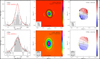 |
Fig. 8 Summary of model predictions of the H30α and H39α lines as in Fig. 3. |
| In the text | |
|
Fig. 9 Model position velocity cuts through the center of along the wind axis (left, PA=0°) and the perpendicular direction (right) as in Fig. 4. |
| In the text | |
|
Fig. B.1 Division of a non homogeneous source into homogeneous cells. The physical conditions, density and temperature, can be considered constant within each cell. |
| In the text | |
|
Fig. B.2 Geometry of the emitting H II region as seen in the coordinate system C (left) and coordinate system C′ (right). The source can be rotated in the C system, but by definition it is not rotated in the C′ system. |
| In the text | |
|
Fig. B.3 Storey & Hummer (1995) NLTE departure coefficients for the Case B and nu=40. |
| In the text | |
|
Fig. B.4 Diagram depicting the procedure to find the value of the NLTE departure coefficient for any arbitrary electron density and temperature. The gray dashed lines indicate the coordinates of the discrete values of density and temperature from the Storey & Hummer (1995) tables (shown as black dots). The orange dashed lines indicate the coordinates of an arbitrary value of electron density and temperature. The solid gray lines indicate interpolation between discrete coefficient values of different densities but the same temperature. The blue dots represent the points connecting the two linear interpolations at an arbitrary electron density. Finally, the orange dot corresponds to the value that Co3RaL uses for an arbitrary electron density and temperature. |
| In the text | |
|
Fig. C.1 Comparison between the predictions by Co3RaL and MORELI for the input model of M 2-9 (LTE, top) and CRL 618 (NLTE, bottom) presented in CSC17 that were designed to reproduce the IRAM-30 m single-dish data reported by these authors – see Sect. C. Left) Synthetic free-free continuum emission spectrum predicted by Co3RaL (black solid line) and MORELI (red dashed line). Data points (circles), shown as a reference, are as in Fig. 1 for M2-9 and as in CSC17 for CRL 618. Middle and Right) Synthetic H30α and H39α 1d spectra (integrated over the emitting region) predicted by Co3RaL (solid black histogram) and MORELI (dashed red histogram). |
| In the text | |
|
Fig. D.1 Synthetic ALMA-like cubes of the free-free continuum emission at 93 GHz (left) and the H30α and H39α lines (middle and right, respectively) obtained from the M2-9 model in CSC17 — see their Table 4 — to be compared with analogous datasets obtained with ALMA in Fig. 1 (top-right) and Fig. 4 (top panels). |
| In the text | |
Current usage metrics show cumulative count of Article Views (full-text article views including HTML views, PDF and ePub downloads, according to the available data) and Abstracts Views on Vision4Press platform.
Data correspond to usage on the plateform after 2015. The current usage metrics is available 48-96 hours after online publication and is updated daily on week days.
Initial download of the metrics may take a while.