| Issue |
A&A
Volume 692, December 2024
|
|
|---|---|---|
| Article Number | A53 | |
| Number of page(s) | 14 | |
| Section | Planets, planetary systems, and small bodies | |
| DOI | https://doi.org/10.1051/0004-6361/202451520 | |
| Published online | 03 December 2024 | |
Impact of solar-wind turbulence on a planetary bow shock
A global 3D simulation
1
Laboratoire Lagrange, Observatoire de la Côte d’Azur, Université Côte d’Azur, CNRS,
Nice,
France
2
Swedish Institute of Space Physics,
Kiruna,
Sweden
3
Institute for Plasma Science and Technology, National Research Council, CNR-ISTP,
Bari,
Italy
4
Space Research Institute, Austrian Academy of Sciences,
Graz,
Austria
5
LPC2E, CNRS, Université d’Orléans, CNES,
Orléans,
France
6
LPP, CNRS/Sorbonne Université/Université Paris-Saclay/Observatoire de Paris/Ecole Polytechnique Institut Polytechnique de Paris,
Palaiseau,
France
7
Dipartimento di Fisica “E. Fermi”, Università di Pisa,
Pisa,
Italy
★ Corresponding author; This email address is being protected from spambots. You need JavaScript enabled to view it.
Received:
15
July
2024
Accepted:
19
October
2024
Abstract
Context. The interaction of the solar-wind plasma with a magnetized planet generates a bow-shaped shock ahead of the wind. Over recent decades, near-Earth spacecraft observations have provided insights into the physics of the bow shock, and the findings suggest that solar-wind intrinsic turbulence influences the bow shock dynamics. On the other hand, theoretical studies, primarily based on global numerical simulations, have not yet investigated the global three-dimensional (3D) interaction between a turbulent solar wind and a planetary magnetosphere. This paper addresses this gap for the first time by presenting an investigation of the global dynamics of this interaction that provides new perspectives on the underlying physical processes.
Aims. We use the newly developed numerical code MENURA to examine how the turbulent nature of the solar wind influences the 3D structure and dynamics of magnetized planetary environments, such as those of Mercury, Earth, and magnetized Earth-like exoplanets.
Methods. We used the hybrid particle-in-cell code MENURA to conduct 3D simulations of the turbulent solar wind and its interaction with an Earth-like magnetized planet through global numerical simulations of the magnetosphere and its surroundings. MENURA runs in parallel on graphics processing units, enabling efficient and self-consistent modeling of turbulence.
Results. By comparison with a case in which the solar wind is laminar, we show that solar-wind turbulence globally influences the shape and dynamics of the bow shock, the magnetosheath structures, and the ion foreshock dynamics. Also, a turbulent solar wind disrupts the coherence of foreshock fluctuations, induces large fluctuations on the quasi-perpendicular surface of the bow shock, facilitates the formation of bubble-like structures near the nose of the bow shock, and modifies the properties of the magnetosheath region.
Conclusions. The turbulent nature of the solar wind impacts the 3D shape and dynamics of the bow shock, magnetosheath, and ion foreshock region. This influence should be taken into account when studying solar-wind-planet interactions in both observations and simulations. We discuss the relevance of our findings for current and future missions launched into the heliosphere.
Key words: plasmas / turbulence / solar wind / Earth / planets and satellites: general
Publisher note: The movie associated with Fig. 6 was missing. It was published as supplementary material on 12 January 2026.
© The Authors 2024
 Open Access article, published by EDP Sciences, under the terms of the Creative Commons Attribution License (https://creativecommons.org/licenses/by/4.0), which permits unrestricted use, distribution, and reproduction in any medium, provided the original work is properly cited.
This article is published in open access under the Subscribe to Open model. This email address is being protected from spambots. You need JavaScript enabled to view it. to support open access publication.
1 Introduction
The solar wind is a supersonic and super-Alfvénic plasma flow that is mainly composed of energetic protons embedded in a large-scale magnetic field; it fills the interplanetary medium and directly interacts with planets, forming a magneto-environment around them. The main features of this environment are a collisionless bow shock, a turbulent magnetosheath, and an elongated magnetosphere downstream from it (Parks et al. 2021; Sibeck & Murphy 2021; Southwood 2021). Depending on the value of θBn, which is the angle between the local shock normal and the direction of the upstream magnetic field, the bow shock can be locally classified as quasi-parallel (θBn < 45°) or quasi-perpendicular (θBn > 45°), with θBn values of around 45° defining a so-called oblique geometry (Jones & Ellison 1991; Schwartz 1998). The existence of these two main shock geometries leads to different plasma kinetic dynamics around the bow-shock region (Burgess & Scholer 2015).
The interaction between planets and the solar wind has been extensively studied over recent decades using numerical simulations. The global interaction between the solar wind and Earthlike magnetospheres has been investigated in the past by means of kinetic hybrid models, where ions are treated as individual kinetic macroparticles and electrons as a charge-neutralizing magnetohydrodynamic fluid. Pioneering hybrid modeling studies include examples focusing on curved collisionless shocks (Thomas & Winske 1990) and the Earth’s magnetosphere (Swift 1995), and have also been focused on the interaction of an interplanetary rotational discontinuity with Earth’s magnetosphere (Lin et al. 1996). Later on, wave behavior (Lin et al. 2001) and velocity distribution functions (Lin & Wang 2002) were studied extensively in the magnetosheath region. A threedimensional (3D) geometry was used to reproduce the basic dynamics of the magnetosphere with the existence of a turbulent magnetosheath medium, an ion foreshock, and waves associated with different regions upstream of the magnetopause (Kallio & Janhunen 2003; Kallio & Janhunen 2004; Trávníček et al. 2007; Müller et al. 2011, 2012; von Alfthan et al. 2014; Modolo et al. 2016; Jarvinen et al. 2020; Aizawa et al. 2021, 2022; Kallio et al. 2022; Teubenbacher et al. 2024). Recently, full, global kinetic particle-in-cell (PIC) simulations of the interaction between the solar wind and a magnetized planet were performed in 2D (Peng et al. 2015) and 3D (Lavorenti et al. 2022; Lapenta et al. 2022; Lavorenti et al. 2023) to investigate the role of electron kinetics in the global interaction of the solar wind with a magnetized planet.
All global models of this kind take the standpoint that the solar-wind plasma dynamics is laminar for the sake of simplicity. Nevertheless, the solar wind is turbulent, with relatively large- amplitude, large-scale magnetic and density fluctuations driven by continuous large-scale energy injection from the Sun. Furthermore, solar wind fluctuations span a large range of spatial and temporal scales (Bruno & Carbone 2013; Kiyani et al. 2015; Verscharen et al. 2019). Therefore, the turbulent solar wind is expected to influence the shock dynamics, as predicted by basic theoretical models (Zank et al. 2002).
Observational studies have focused on the dynamics and turbulent nature of the solar wind and its connection to the bow shock, magnetosheath, and magnetosphere dynamics (see, e.g., Rakhmanova et al. 2023, and references therein). In particular, observations have shown that geomagnetic activity depends on internal magnetospheric processes and solar wind conditions (D’Amicis et al. 2020; Guio & Pécseli 2021a,b). Complementary to observations, local simulations of the interaction between solar-wind turbulence and an interplanetary shock are very recent. As opposed to global simulations, these were performed with the focus placed on a relatively small portion of the shockinteraction region. Also, the authors did not take into account the global curved nature of a planetary shock, and used one wall of the simulation as a fully reflective boundary. Trotta et al. (2021) showed that turbulent fluctuations in the upstream region enhance particle acceleration at the shock front, leading to a diffusive spread of the particles in velocity space. This result has been supported by observations of an increase in the magnetic helicity downstream of the shock as turbulent structures are compressed while they are transmitted across the quasiperpendicular shock (Guo et al. 2021; Trotta et al. 2022). Local hybrid PIC simulations have also been used to study the interaction of multiple current sheets with a shock wave, with the authors discussing the implication of this interaction on particle acceleration in the downstream shock region (Nakanotani et al. 2021). Further hybrid PIC simulations have confirmed the role of upstream turbulence as a scattering agent to promote diffusive shock acceleration (Nakanotani et al. 2022). More recently, by coupling turbulent magnetohydrodynamic fields and local quasiperpendicular hybrid kinetic 3D simulations, Trotta et al. (2023) showed that turbulence increases fluctuations at the shock interface and the isotropization of the magnetic field spectra in the downstream region close to the bow shock.
However, none of the above studies investigated the global response of a planetary magnetosphere to solar-wind turbulence. The numerical code that we use in the present study, namely MENURA (Behar et al. 2022), is specifically designed for this purpose. MENURA can self-consistently model a fully developed turbulent solar wind interacting with a planet and was recently used by Behar & Henri (2023) to show that, in 2D, the turbulence of the solar wind significantly modifies the dynamics of the induced magnetosphere of comets.
Here, we present the results of the first 3D hybrid simulation of the interaction between a turbulent solar wind and a planetary magnetosphere that is about three times smaller than the terrestrial one. For the first time, we show how the turbulent nature of the solar wind affects the global shape and dynamics of the bow shock, the fluctuations in the magnetosheath, and the ion foreshock region.
The paper is organized as follows. In Sect. 2 we describe the model and the parameters of the simulations conducted with MENURA. In Sect. 3 we discuss the shape of the bow shock and its dynamics. We focus specifically on the ion foreshock and the structures locally created by the upstream turbulence as examples of the kinetic effects – captured by MENURA – acting on both quasi-parallel and quasi-perpendicular regions of the bow shock In Sect. 4 we present our conclusions, and discuss future perspectives to continue this line of study.
2 The model
We used the 3D hybrid kinetic PIC code MENURA to simulate the interaction of a turbulent solar wind with a planetary magnetosphere. A detailed code description is available in Behar et al. (2022), and an example of its application in a 2D geometry is described in Behar & Henri (2023). In the present work, we use the 3D version of the code. MENURA provides a kinetic description of ion dynamics and employs a generalized Ohm’s law coupled to a polytropic closure for the massless electrons. MENURA uses the current advanced method (CAM) scheme (Matthews 1994) commonly employed in PIC hybrid codes as well as more recently in hybrid Eulerian Vlasov codes (Valentini et al. 2007).
The present study was conducted in two successive steps. First, we performed a 3D simulation of the decaying turbulence of solar wind using periodic boundary conditions. This simulation follows the solar-wind evolution until a quasi-stationary state is achieved and the turbulence is fully developed. Second, we used the last iteration step of the turbulent decay simulation as the initial condition of a new run in which we simulated the interaction of this turbulent solar wind with a magnetized planet. More details on treating boundary conditions for this second step are described in Behar et al. (2022) and Behar & Henri (2023). Additionally, a reference simulation was performed using laminar solar-wind conditions to properly assess the effects of solar-wind turbulence on the interaction with the planetary obstacle.
In both steps, the solar wind and planetary plasma dynamics equations are solved in the solar-wind reference frame. Unlike the object-centred reference frame used in other codes with similar scientific purposes (von Alfthan et al. 2014; Grandin et al. 2023; Karimabadi et al. 2006), solving equations in the solarwind reference frame enables the introduction of a solar-wind magnetic field that varies in space and time. This condition is necessary in order to inject a well-defined, fully developed, self- consistently generated turbulent flow that includes, for example, magnetic vortices.
In the following, we describe the initial conditions and parameters of these two successive simulations, which we named Sim 1 and Sim 2.1, and the reference laminar run, which we named Sim 2.2. Table 1 summarises the input parameters of the simulations.
2.1 Decaying simulation of solar-wind turbulence (Sim 1)
In this simulation, the solar wind consists of one ion species (protons) and massless neutralizing electrons. The simulation domain is a Cartesian box of equal size Lbox = LX = LY = LZ = 2000 di in the three spatial directions that is discretized in 400 cells in each direction with a spatial resolution of ∆x = 5di, with di being the solar-wind proton inertial length. We populate each cell with 600 macroparticles to ensure a statistically satisfactory representation of the ion distribution function. The simulation’s time step is  , with Ωci being the solar-wind proton gyrofrequency, which is computed using the solar-wind mean magnetic field. Consequently, these simulation parameters are such that ion scales are poorly resolved spatially and temporally. Such a resolution is imposed by computational constraints; however, in this study, we do not specifically focus on the dynamics at the ion and sub-ion scale but rather on phenomena just below the smallest magnetohydrodynamic scales, approaching the ion kinetic scales, while enabling us to describe some kinetic features such as a supercritical bow shock and the associated reflected ions in the foreshock. The initial equilibrium condition is made of a solar-wind plasma with homogeneous density and temperature, permeated by a homogeneous, oblique (to the solarwind flow) mean magnetic field B0 (see Table 1). At equilibrium, the plasma beta, that is, the ratio of ion kinetic and magnetic pressures, is βi = 0.5, and the ion-to-electron temperature ratio is Ti/ Te = 1, resulting in β = βi + βe = 1. We impose an isothermal closure on electrons, corresponding to an adiabatic index of γe = 1. We perturb this equilibrium with magnetic and velocity fluctuations at large scales. The initial velocity fluctuations are incompressible following ∇ ⋅ v = 0. The initial perturbation is made of sinusoidal fluctuations with a polarization orthogonal to both the mean field and the wavevector k. The wavevectors are directed along the three Cartesian directions and all wavevectors within the range [kmin, kmax] = [2π/Lbox, 5 ⋅ 2π/Lbox] are populated. The phases are random and different for the velocity and magnetic fluctuations. The root mean square of the initial magnetic and velocity fluctuations is δB0/B0 = δv0/CA = 0.54, where CA is the background Alfvén speed in normalized units.
The magnetic field lines and the total current density in the simulation box at the end of the decaying turbulence simulation are shown in Fig. 1a. The anisotropy in the magnetic field fluctuations is evident from the elongated shape of the current structures aligned parallel to the mean solar-wind magnetic field.
The time evolution of the charge current fluctuations Jrms, defined as its root mean square (RMS), is shown in Fig. 1b. The vertical dashed line indicates the time at which the decaying turbulence simulation is fully developed, so that it can then be injected into the magnetized planet simulation. We identify it with the time when the RMS current saturates. At the end of this first simulation, the RMS value of the final perturbation is δB/B0 = 0.45 and δv/CA = 0.33, where δB and δv are the magnetic and velocity RMS values and B0 is the background magnetic field.
We computed the parallel and perpendicular (to the mean solar-wind magnetic field direction) spectra of magnetic and velocity fluctuations, as shown in Fig. 1c. The magnetic field follows a power-law trend with a spectral slope that is consistent with the expected Kolmogorov decay of –5/3. At smaller scales, closer to one di, the spectral trend changes under the effect of both the numerical dissipation (hyper-resistivity) and dispersive and kinetic ion physics (Matteini et al. 2016).
The electric and magnetic fields as well as the plasma distribution function from the decaying turbulence simulation at time  are used to initialize the second simulation of our model (Sim 2.1).
Input parameters of the simulations.
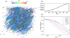 |
Fig. 1 Characteristics of the decaying simulation of solar-wind turbulence (Sim 1). (a) Current density normalized to its RMS Jrms (color map) and magnetic field lines (orange) in the full 3D plasma box. (b) Box-averaged square current density J2 as a function of time. The vertical dashed line marks the time of the snapshot ( |

2.2 Interaction between a magnetized planet and the solar-wind turbulent dynamics (Sim 2.1)
In this second simulation, we modeled the interaction between a solar wind – with fully developed turbulent dynamics resulting from Sim 1 – and a magnetized planet. The magnetized planet is modeled as a perfectly absorbing body – with entering plasma being removed from the simulation – together with a permanent magnetic dipole, taken as an external magnetic field.
As the computation is performed in the solar-wind frame, the planet is moving in the simulation domain at a speed that is opposite to that of the solar wind. To maintain the planet at a fixed position in the simulation domain, we continuously shift the domain sideways (in the + X direction). Consistently, the dipole field is recalculated each time the simulation box moves. Our choice of reference frame requires the addition of another term in Faraday’s law that corresponds to a Lorentz transformation. To our knowledge, this is the first time a non-fixed reference frame has been used for this type of application.
For a small plasma beta “β”, the critical mach number Mcrit of a shock varies between 1.53 (for quasi-parallel) and 2.76 (for quasi-perpendicular shock), and for β > 1, Mcrit ~ 1 for all shock normal angles (Kennel 1987). This means planetary bow shocks in the heliosphere are almost always supercritical. Therefore, we concentrate on a supercritical bow shock in this study, setting MA = 10. We note that for a supercritical shock, wave-particle interactions dominate the dissipation processes; instead, in sub- critical shock, the foreshock structure upstream of quasi-parallel shocks, for instance, would not be expected (Burgess & Scholer 2015).
In the simulation box, the planet’s center is kept at coordinates (XP, YP, ZP) = (3Lbox/8, Lbox/2, Lbox/2) = (750, 1000, 1000) di, with Lbox being the size of the box in any direction in units of di. The dipole value is chosen by fixing the distance from the planet center to the magnetopause Dp. This parameter has proven to be an effective method for characterizing the magnetospheric structure as a function of dipole strength (Omidi et al. 2004; Karimabadi et al. 2014). In the present work, for the sake of reducing the computational effort, we use Dp = 200 di, which is a smaller value than the real value at Earth (Dp,Earth ~ 640 di). As pointed out in Omidi et al. (2004), simulations with Dp of greater than about 20 – which is one order of magnitude smaller than the one we use – have Earthlike characteristics both on the dayside and in the magnetotail regions. The smaller size of the magnetosphere and magnetosheath reduces the transit time of the plasma inside the magnetosheath by a factor of about 3 with respect to the Earth. This may affect the development of waves in the region, such as wave modes with a relatively low growth rate, as they may not have time to develop before reaching the magnetopause. However, this work is the first step in studying how turbulent solar wind globally affects the different large-scale frontiers in a planetary magneto-environment.
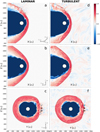 |
Fig. 2 Comparison of ion density in logarithmic scale between laminar (a–c) and turbulent (d–f) simulations at |

2.3 Interaction between a magnetized planet and the solar wind laminar dynamics (Sim 2.2)
To properly assess the impact of the turbulent nature of the solar wind on a magnetosphere, it is necessary to compare its effect to that of an upstream solar wind that would be laminar. For this purpose, we ran a third reference simulation in which the planet interacts with a laminar solar wind. In this case, the planet moves into a homogeneous solar wind with plasma density and temperature equal to those chosen as the initial condition of Sim 1. The solar-wind magnetic field is also homogeneous and equal to Bsw. All other simulation parameters, including planet parameters and spatial and temporal resolution, are identical to those of Sim 2.1.
3 Impact of a turbulent solar wind on a planetary bow shock
In the following, we compare the turbulent (Sim 2.1) and laminar (Sim 2.2) simulations to highlight the effects that the turbulent nature of the solar wind has on the magneto-environment of a planet. To compare the structure and dynamics of the solar wind, the shock, and the magnetosheath in the two simulations, we present maps of relevant quantities in three perpendicular planes intersecting the center of the planet, located at coordinates (XP, YP, ZP).
Figures 2, 3, and 4 present global maps of the plasma density, the magnetic field magnitude, and the proton bulk speed, respectively: the left column (panels a–c) shows the laminar solar wind case results, whereas the right column (panels d–f) shows the turbulent solar wind case at the same simulation time  . Density is normalized to the solar-wind proton density, the magnetic field is normalized to the solar-wind magnetic field, and the proton bulk speed is normalized to the Alfvén speed (see Table 1). For both turbulent and laminar simulations, the bow shock, magnetosheath, and magnetopause regions can be clearly identified, with the quasi-parallel (Y > 1400 di) and quasi-perpendicular (Y < 800 di) sides of the shock having shapes and extents that are in good qualitative agreement with other global simulations (Turc et al. 2023). Closer to the planet, the regions where ions are seen flowing within the magnetosphere of the planet take the shape of highly structured cones in 3D (see Fig. 2a in the X-Y plane at Z = Zp, with ZP being the position of the planet’s center), closely mimicking the Earth’s plasma cusps. These “cusps” appear relatively less defined in the turbulent solar wind case, owing to the less homogeneous magnetosheath (Fig. 2b). The following sections provide a detailed description of how the turbulent nature of the solar wind shapes these boundaries and regions.
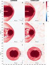 |
Fig. 3 Comparison of the magnetic field amplitude in logarithm scale between laminar and turbulent simulations at |

3.1 Shape of the bow shock
To facilitate comparisons of the shape of the bow shock between simulations with and without turbulence in the solar wind, we built a simple proxy of the 3D position of the shock surface saved at high temporal cadence during a numerical run. This proxy is defined using the plasma density: for each (Y, Z) coordinate, the position of the bow shock is estimated to be the first position along the X direction at which the density jumps above a value of 101/4, which is about 1.8 times the solar-wind background value, which is chosen as an intermediate value between the upstream solar wind and the downstream magnetosheath plasma.
The position of the shock in the laminar solar wind case (Sim 2.2) is shown in Fig. 2 by the thin solid black line within each plane. The same line is superimposed onto the results of the turbulent case (Sim 2.1) as a baseline for comparison of the laminar and turbulent solar wind–planet simulations. Moreover, the same bow shock position in the laminar case is superimposed onto the magnetic field maps (Fig. 3), showing how well it captures the sharp transition between the upstream solar-wind magnetic field (in white) and the compressed downstream magnetic field and denser magnetosheath (in red). Similarly, this sharp transition is seen on the proton bulk speed maps (Fig. 4), where the solar wind (in white) is abruptly slowed down to subsonic speeds at and downstream of the shock (blue hues).
When observing the quasi-perpendicular region of the bow shock, the density maps in Figs. 2a–f show that the shock surface is inflated or deflated with respect to the laminar case when the impinging initial solar wind is turbulent. This feature is also confirmed by the magnetic field (Fig. 3) and the proton bulk speed maps (Fig. 4). These fluctuations of the quasi-perpendicular bow shock surface result from local inhomogeneities in the solarwind bulk dynamic pressure, which stem from the turbulent nature of the initial solar-wind condition in Sim 2.1: turbulence causes certain regions to experience higher or lower values of solar-wind dynamic pressure compared to the laminar case (Sim 2.2).
The difference between the bow shock’s location in the two runs is most pronounced for the quasi-parallel shock. In this region, the shock surface proxy varies widely, as seen for Y ≳ 1300 di in Fig. 2a and at Y ∼ 1500 di in the corresponding perpendicular plane in Fig. 2c, the laminar case. Nevertheless, the sharp and well-defined transition between the upstream and quasi-parallel downstream domains in the laminar case is mostly lost in the turbulent case due to fluctuations in the solar wind that locally change the magnetic field orientation with respect to the shock normal. In this way, the density variation proxy used for the laminar case cannot capture the highly variable quasi-parallel shock interface in the turbulent case. However, this proxy remains useful for highlighting the extent to which turbulence changes the quasi-parallel shock location and shape.
In the density maps in Fig. 2, we observe that the compression downstream of the quasi-parallel shock is less pronounced in the turbulent case (Fig. 2d) and the structure of the bow shock is significantly more perturbed than in the laminar case (Figs. 2c,f). For Y > 1600 di, it becomes difficult to identify the exact location of the quasi-parallel shock boundary (Fig. 2d).
These differences are clearly shown in Fig. 5 where the bow shock is visualized in 3D, setting a transparency threshold of nth = 101/4n0 on the plasma density. While in the laminar case (Fig. 5a), the shock boundary is mainly smooth over the entire corresponding quasi-perpendicular surface, for the turbulent simulation (Fig. 5b), large fluctuations are presented all over the bow shock. The quasi-parallel region is more easily identified in the laminar case, where the fluctuations delimit a clear area around the north pole region that corresponds to the foot points from where magnetic field lines (in red) parallel to the local shock normal are emerging. In contrast, the corresponding quasi-parallel region is not well delimited for the turbulent case, and the magnetic field lines do not appear aligned as they are in the laminar case. This feature affects the dynamics of the ion foreshock, as discussed in more detail in Sect. 3.4.
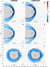 |
Fig. 4 Comparison of the proton bulk speed Up between laminar (left column) and turbulent solar wind simulations (right column) at |

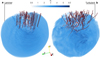 |
Fig. 5 Three-dimensional rendering of the bow shock for the (a) laminar and (b) turbulent solar wind cases. Ion density is represented in blue hues. A threshold density of nth = 101/4n0 is applied, such that all regions in which ni < nth are made transparent. A linear transparency profile is applied from ni = nth to ni = 6n0, and so low-density regions are more transparent than high-density ones. Upstream magnetic field lines crossing the ion foreshock regions are drawn in red. |
3.2 Dynamics of the bow shock
As already described, the proxy of the bow shock position introduced in the previous section is computed at runtime at a high cadence. This enables a high-resolution analysis of the time evolution of the bow shock shape as driven by the solar-wind dynamics. This analysis is shown in Fig. 6. To reduce the dimension of the problem, we first considered the 1D time-averaged position over the whole simulation of the bow shock for the coordinates (YP, Z). We then calculated the deviation of the bow shock position along the Sun–planet direction X from its time- averaged value. The time evolution of this deviation is shown in red (blue) tones, highlighting the times and positions at which the shock location is upstream (downstream) of its average position. This is done for both the laminar (Fig. 6a) and turbulent (Fig. 6b) solar-wind dynamics. The deviations from the average position are displayed in the range going from –10 di to +10 di. We note that the turbulence of the impinging solar wind induces oscillations of the shock surface of far greater amplitude. The variance of the values shown in Fig. 6a is 0.8 di, while a greater variance of 2.0 di is found in the turbulent case. Second, we present the deformation of the full 3D bow shock surface, as depicted in Figs. 6c and d by showing the planar projections of the full 3D shock surface position with respect to its time- averaged position. This is shown for time  , for both laminar (Fig. 6c) and turbulent (Fig. 6d) solar-wind dynamics. A video reporting the evolution of Figs. 6c and d as a function of time is available online.
This representation of the bow shock deformation is similar to that of the position of a vibrating tambourine skin under the drumming action of the impinging solar wind. We observe local and global oscillations of the shock position. In the laminar solar wind dynamics case, the bow shock deformation is first observed at the bow shock nose and subsequently propagates from the nose toward the flanks along the surface of the shock, creating the “butterfly”-shaped propagating structures in the Z–t space observed in the top panels. In contrast, for the turbulent solar wind dynamics case, the bow shock deformation originates from multiple regions (not only the nose) depending on the solar-wind dynamics and the local conditions at the shock. These deformations later propagate toward the flanks along the surface of the shock, generating an even more complex deformation pattern. This dynamics is reminiscent of the ubiquitous rippling observations at the Earth’s quasi-parallel (Pollock et al. 2022), quasi-perpendicular (Moullard et al. 2006), and oblique (Gingell et al. 2017) bow shock.
Third, we look more quantitatively at the shock surface variations in each region around the planet. The quasi-parallel shock region exhibits significant variability, regardless of the initial solar wind conditions imposed in the simulations. The oblique and quasi-perpendicular shock surface variations are strongly enhanced in the turbulent solar wind case, with amplitudes reaching ±10di, whereas in the laminar case, maximum amplitudes are much weaker (±2di). Beyond this much greater motion of the shock surface, turbulence is also responsible for the peculiar dynamics observed in confined regions of the shock front. At  , close to the nose of the shock around Z ~ 800 di, a small “spot” (circled in black in Fig. 6b) departing from the average shock position is seen on the time series for the turbulent simulation. This transient structure is located at the bow shock interface around coordinates (1000, 800) di in the X–Z plane in Figs. 2e, 3e, and 4e and propagates along the shock’s surface and inside the magnetosheath (Fig. 6b). We show a zoom-in plot of this highly dynamic structure in Fig. 7, with density, magnetic field, and bulk speeds corresponding to a snapshot of the simulation when the structure has fully formed. It appears as a localized “bubble” of lower magnetic field and lower-density plasma enclosed by high-magnetic field, high-density plasma boundaries. This suggests that, locally, a bubble of shocked solarwind plasma can impulsively penetrate inside the magnetosheath and start interacting with the local plasma there. Adding complexity to this picture, Fig. 7c also shows that the bulk speed inside this bubble is as low as its immediate surroundings, with plasma already decelerated to magnetosheath-like speeds, whereas its density and magnetic field amplitude are closer to solar-wind values. Although an analysis of this precise structure and others found in the quasi-perpendicular shock of the turbulent simulation is beyond the scope of this study, it is interesting to note that such signatures, which are characteristic of rippling and reformation processes that are usually found in quasi-parallel shocks, have also been seen in local hybrid simulations of plasma turbulence interacting with quasi-perpendicular shocks (Trotta et al. 2022). In the Appendix, we report a complementary visualization tool that we have developed to analyze global planetary simulations based on a tomography of the simulation domain.
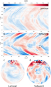 |
Fig. 6 Temporal evolution of the deviation from the time-averaged bow shock position for the coordinates (YP, Z) in the laminar (a) and turbulent (b) case. The color code provides the deviation in di . The black circle points to the “bubble” appearing around (1000, 800) di in Figs. 2e, 3e, and 4e and reported in Fig. 7. The planar projection of the full 3D shock surface deviation at |

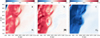 |
Fig. 7 Transient structure along the location of the bow shock in the X-Z plane of the turbulent simulation at |

3.3 Magnetosheath structure
As can be seen in Fig. 2 (plasma density), the thickness of the magnetosheath downstream of the quasi-parallel shock is smaller than downstream of the quasi-perpendicular shock for both laminar and turbulent solar-wind conditions. This is consistent with Time History of Events and Macroscale Interactions During Substorms (THEMIS) spacecraft observations over a five-year period (Dimmock & Nykyri 2013), which uncovered an asymmetry in the Earth’s magnetosheath between the dawn and dusk regions due to the nominal Parker spiral geometry. When comparing the laminar and turbulent runs, this asymmetry persists.
In Figs. 2a and c and 3a and c for the laminar run (left column), the magnetosheath region also exhibits large fluctuations in density and magnetic field magnitude, which fill all of the magnetosheaths, as expected from observations (Narita et al. 2021). Fluctuations are more coherent in the quasi-perpendicular region than in the quasi-parallel region, where this coherence is mostly lost, and fluctuations become larger in size and amplitude. In the turbulent case, some of that coherence is further lost, as can be observed when comparing both columns of Figs. 2 and 3. This is very similar to what has been seen in numerical simulations of solar wind–comet interactions when considering the turbulent nature of the solar wind (Behar & Henri 2023).
The additional loss of coherence in fluctuations in the quasiperpendicular magnetosheath due to solar-wind turbulence may be explained by the transmission of large-scale solar-wind turbulence structures across the shock. These structures are observed clearly in some regions immediately downstream of the bow shock; for example, around coordinates (400, 1100) di and (1000, 400) di in the Y–Z plane in Figs. 2f, 3f, and 4f. However, another possible explanation for the observed structures downstream of the quasi-perpendicular shock is the interaction of self-generated transients at the quasi-perpendicular shock, such as the high-density high-B-field “bubble” previously mentioned in Sect. 3.2 around (X, Z) ≈ (1000, 800) di in Figs. 2e, 3e, and 4e.
For the quasi-parallel region, the presence of upstream solarwind turbulence increases the size and magnitude of the fluctuations in the magnetosheath, as can be seen for Y ≳ 1300 di in panel (d), and for Y ∼ 1400 di and 700 ≲ Z ≲ 1300 di in panel (f) of Figs. 2 and 3. In this geometry, the fluctuations occurring on the downstream and upstream sides of the shock were already present in the laminar case, albeit in a less developed and intense manner (Figs. 2c and 3c). Disentangling the effects due solely to solar-wind turbulence from those inherited from the basic laminar conditions will require a dedicated analysis, which is outside the scope of the present study. These aspects will be explored in future research.
Figure 4 shows how the plasma in the wake of the bow shock is slowed down to speeds significantly below the upstream solar-wind bulk speed of Usw = 10 CA, with white marking the reference solar-wind speed. In the quasi-perpendicular side of the magnetosheath in the laminar case (Fig. 4a), fluctuations in plasma speed provide a “baseline” level of the magnetosheath natural turbulence, with striations appearing perpendicular to the shock surface in the immediate wake of the shock front (as clearly seen in Fig. 4c). In contrast, bulk plasma speed fluctuations are much increased for the turbulent case as compared to the laminar case, with large wavy structures developing almost parallel to the shock surface behind the terminator line (Fig. 4d) and superimposed on the natural turbulence of the magnetosheath (Fig. 4f). Deeper in the quasi-perpendicular magnetosheath, the plasma is further compressed, and witnesses increased speed near the modeled magnetopause. In general, downstream of the quasi-perpendicular shock, the plasma velocity fluctuates much more in the turbulent case than in the laminar case, as especially seen in the flanks (Fig. 4f), with large defined structures possibly modulated by the global-scale turbulence upstream of the shock.
On the quasi-parallel side of the magnetosheath, the conclusions already drawn for Figs. 2 and 3 hold: fluctuations in the ion foreshock region increase substantially, with a loss of coherence of the backstreaming ions that create the characteristic ultra low-frequency (ULF) waves populating the foreshock. Streams of low bulk speeds (in dark blue, Fig. 4d) appear upstream of the shock, corresponding to relatively low magnetic field intensities and low plasma densities.
While the solar wind mainly crosses the quasi-perpendicular part of the bow shock, some of it is actually reflected in the quasi-parallel part, forming the so-called ion foreshock region upstream of the quasi-parallel shock region. We focus on this region below.
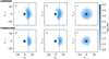 |
Fig. 8 Ion VDF for the laminar (panels a–c) and turbulent case (panels d–f) in logarithmic scale. The VDF is plotted in a reference frame aligned with the local magnetic field and moving with the solar wind. The plots show the number of macroparticles integrated in the out-of-plane direction. The blue dashed line corresponds to the opposite of the solar-wind speed in the planet reference frame. |
3.4 Dynamics within the ion foreshock
In this section, we discuss the influence of the turbulent nature of the solar wind on the ion foreshock. Because the bow shock is supercritical and collisionless, solar-wind ions are expected to be reflected in the bow shock region quasi-parallel to the solar-windmagnetic field. This is well modeled in our kinetic hybrid simulations, and the resulting ion foreshock is observed upstream of the shock, for Y > 1400 di in panels a and d of Figs. 2, 3, and 4, as expected.
The solar-wind ions reflected by the bow shock are seen in the ion velocity distribution functions (VDFs) shown in Fig. 8, both for the laminar and turbulent solar wind. The VDF is computed in a cubic box centered on r0,vdf(x, y, z) = (860, 1620, 1020)di with a size of 40di × 40di × 40di. The box size is chosen to ensure enough statistics on the particle beam. Figure 8 displays the VDFs in a reference frame oriented as  , and
, and  , where B and V are the box-averaged values of the local magnetic and ion velocity fields, that is, in the box where the VDF is computed. In both laminar and turbulent solar-wind conditions, we observe the characteristic solar-wind core population centered at the origin of the coordinates and a less populated beam moving on average in the
  direction, as indicated by the dashed blue line. The beam velocity is vbeam = –Usw = 10 in Alfvén speed (code) units. The beam width is comparable in the two perpendicular directions and the VDF is thus close to gyrotropic (Figs. 8c,f). The two VDFs (in laminar and turbulent solar wind conditions) appear quite similar in the selected location. However, the particle density in the beam corresponding to reflected particles is reduced in the turbulent case compared to the laminar one. We observed this feature everywhere in the ion foreshock.
The presence of solar-wind turbulence influences the spatial distribution of the reflected beam itself. Figure 9 shows its density Nb in the foreshock region for the two simulations. The plot is obtained using the following procedure. The VDF is computed in boxes of 40di × 40di × 40di, forming a grid in the physical space. For each set of particles located inside one box, particles with a speed of |v| > 5 CA – where CA is the Alfvén speed in the pristine solar wind in our simulation – are used to compute the beam density. We observe that the fluctuations in the reflected beam density are much more pronounced in the turbulent case (Fig. 9b) than in the laminar (Fig. 9a) case. We argue that this behavior is due to two factors: in the turbulent case as compared with the laminar, (i) the foreshock base region is more inhomogeneous (as shown in Fig. 5), and (ii) the magnetic field line diffusion in the direction perpendicular to the mean magnetic field is enhanced. The combination of these two processes influences the transport of particle beams, resulting in a loss of coherence of the beam itself when moving away from the bow shock and a more patchy density distribution in the turbulent case.
To elucidate the global picture of this process, Fig. 5 shows a 3D rendering of the magnetic field lines in the foreshock region. We observe that the magnetic field lines in the laminar case appear to align with the direction of the solar-wind magnetic field, oscillating due to beam-induced waves in the foreshock that resemble the right-hand polarized ULF waves seen at Earth and arising from wave–particle interactions (Narita et al. 2004). In contrast, the field line topology appears much more complex in the turbulent case. The ULF oscillations are observed only close to the shock base and disappear while moving away from it toward the solar wind. Moreover, in the turbulent case, some magnetic field lines crossing the foreshock region have footprints outside the quasi-parallel shock base.
This implies that part of the plasma in the foreshock region comes from outside the foreshock where particle reflection has been less efficient. This complex magnetic topology results in the patchy distribution of the ion beam density in the foreshock region, as reported in Fig. 9b.
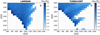 |
Fig. 9 Ion beam density Nb in the foreshock region for (a) laminar and (b) turbulent solar-wind dynamics conditions. The color bar is in logarithmic scale; Nb<10 in white regions. |
4 Conclusion
We performed the first 3D global simulation of the interaction between a turbulent solar wind and a magnetized planet. We investigated the influence of turbulence on the shape and dynamics of the bow shock, the structure of the magnetosheath, and the ion foreshock.
Regarding the bow shock dynamics, larger fluctuations in the shock’s position are observed as compared to the laminar case. Additionally, we show that while in the laminar case the deformation of the bow shock outside of the quasi-parallel region originates solely at the nose of the shock, in the turbulent case deformations are triggered in multiple regions depending on solar-wind dynamics and local conditions. These deformations propagate along the shock’s surface toward the flanks, resulting in a more complex pattern. Consequently, the oscillations in the surfaces of oblique and quasi-perpendicular shocks are significantly amplified in turbulent solar-wind conditions. Our study also shows that bubble-like plasma structures can form in the quasi-perpendicular shock region, where they start interacting with the local plasma in the magnetosheath. Further investigation into this phenomenon is deferred to future research.
The magnetosheath structure under laminar and turbulent solar-wind conditions exhibits similar behavior with a spatial asymmetry between the quasi-parallel and quasi-perpendicular sides of the shock, which is in agreement with observational statistical studies (Dimmock & Nykyri 2013). The main effect of the turbulent solar-wind dynamics on the magnetosheath is, on average, to diminish the coherence of the B-field and density fluctuations and enhance their amplitude, which is qualitatively consistent with the observed transmission through the bow shock of the turbulence inherited from the solar wind. In the ion bulk speeds, we also observed in the turbulent case the appearance of long wavy structures elongated almost parallel to the shock surface, with larger ion speed fluctuations and locally faster speeds than in the laminar case. In the future, we aim to carry out a more detailed exploration of how 3D solar wind structures are processed by the shock (following, e.g., Trotta et al. 2022) and to investigate whether the relaxed equilibrium states typical of the turbulent phenomenology and observed in the magnetosheath are locally generated or may originate from the solar wind (Pecora et al. 2023).
In the ion foreshock region, the presence of upstream turbulence influences the spatial properties of the reflected ion beam. Specifically, this ion beam in the turbulent case is more inhomogeneously distributed in space and extends less far upstream from the shock than in the laminar case due to the enhanced complexity of the magnetic field lines. Furthermore, we show that turbulence and beam-induced fluctuations in the foreshock region may exist for the solar-wind turbulence level considered in our simulation. We may expect their presence and importance in the foreshock region to vary with the amplitude of the turbulence advected by the solar wind. A systematic study of the interplay between the two will require more simulations where the amplitude of the upstream solar-wind turbulence is varied; this is also left for future work.
MENURA’s distinctive approach, reproducing the global interaction of a turbulent solar wind with compact objects, including planetary magnetospheres – induced or not –, marks a significant advancement in our theoretical description of the near-Earth environment. Multi-satellite missions, such as ESA’s Cluster, NASA’s Time History of Events and Macroscale Interactions during Substorms (THEMIS), and, more recently, NASA’s Magnetospheric Multiscale Mission (MMS), all continue to investigate the Earth’s magnetosphere, magnetosheath, and nearEarth solar wind with increasing temporal and spatial resolution, and may benefit from numerical work such as that presented here.
Further, MENURA is a parallel code based on and running on graphics processing units (GPUs). We expect that, in the future, due to increased computational power, simulation at the full Earth scale may become feasible. Planets like Jupiter and Saturn remain too big to model with the computational resources presently available. However, the interaction between a turbulent plasma (solar wind) and a bow shock is expected to be similar for a giant planet since the thickness of the collisionless shock remains at ion kinetic scales. Therefore, this paper is relevant for the physics that occurs upstream and immediately downstream of the shocks of giant planets. Meanwhile, planetary magnetospheres of smaller sizes may be studied with full-scale simulations. These upcoming simulations are timely, considering that the ESA-JAXA (Japan Aerospace Xploration Agency)/BepiColombo mission will reach Mercury in November 2026. Additionally, due to the ease with which different temporally variable initial conditions can be imposed in MENURA, future studies could also include the modeling of magnetic clouds (coming from coronal mass ejections) and stream interaction regions. Finally, numerical studies of global dynamics that consider kinetic effects, such as that presented in this work, may also be relevant to many other astrophysical systems constituting a compact object – with or without an intrinsic magnetic field – interacting with a non-laminar flow.
Movie
Movie 1 associated with Fig. 6 Access Supplementary Material
Acknowledgements
E.B. acknowledges support from the Swedish National Research Council, Grant 2019-06289. This work was granted access to the HPC resources of IDRIS under the allocation 2021-AP010412309 made by GENCI. P.H. acknowledges support from CNES APR. This work was granted access to the HPC resources of IDRIS under the allocation 2024-AD010412990R1 made by GENCI. C.S. Wedlund is funded by the Austrian Science Fund (FWF) 10.55776/P35954. L.P. was supported by the Austrian Science Fund (FWF): P 33285-N. F.P. acknowledges support from the National Research Council (CNR) Short Term Mobility (STM) 2023 program and from the Research Foundation – Flanders (FWO) Junior research project on fundamental research G020224N. We acknowledge the CINECA award under the ISCRA initiative, for the availability of high performance computing resources and support.
Appendix A 3D shape of the magnetic environment of an Earth-like planet interacting with a laminar and a turbulent solar wind
To visualize the differences between the laminar and turbulent case in 3D, we show in Fig. A.1 a “tomographic” view of the density for both simulations, composed of consecutive space slices perpendicular to the Sun-planet line, i.e. Y–Z planes along X. The differences in the solar-wind region for the two cases are evident. The laminar simulation, being devoid of any solar-wind turbulence, only shows the expected foreshock fluctuations generated upstream of the quasi-parallel shock. Instead, fluctuations larger in size and magnitude are present in the turbulent case. The bow shock for the turbulent case is more deformed than in the laminar case. That can be noticed when inspecting the shape of the boundary in the quasi-perpendicular shock region: in the turbulent case, it is less “rounded” and more extended in space. When scrutinizing the turbulent simulation results, the spatial slices show that some upstream turbulent patterns are transmitted across the quasi-perpendicular shock. Finally, in the turbulent case, the magnetosheath is compressed or expanded due to turbulent fluctuations with respect to the laminar case. Inside the magnetosheath, the coherent structure patterns present in the quasi-perpendicular region of the laminar case are absent or blurred when compared to the turbulent simulation.
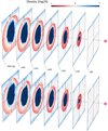 |
Fig. A.1 Tomographic view of the ion density in consecutive space slices perpendicular to the Sun-planet line. The x axis spans 50 to 990 di. |
References
- Aizawa, S., Griton, L., Fatemi, S., et al. 2021, Planet. Space Sci., 198, 105176 [NASA ADS] [CrossRef] [Google Scholar]
- Aizawa, S., Persson, M., Menez, T., et al. 2022, Planet. Space Sci., 218, 105499 [NASA ADS] [CrossRef] [Google Scholar]
- Behar, E., & Henri, P. 2023, A&A, 671, A144 [NASA ADS] [CrossRef] [EDP Sciences] [Google Scholar]
- Behar, E., Fatemi, S., Henri, P., & Holmström, M. 2022, Ann. Geophys., 40, 281 [NASA ADS] [CrossRef] [Google Scholar]
- Bruno, R., & Carbone, V. 2013, Liv. Rev. Sol. Phys., 10, 2 [Google Scholar]
- Burgess, D., & Scholer, M. 2015, Collisionless Shocks in Space Plas-mas:Structure and Accelerated Particles, Cambridge Atmospheric and Space Science Series (Cambridge: Cambridge University Press) [Google Scholar]
- Dimmock, A. P., & Nykyri, K. 2013, J. Geophys. Res.: Space Phys., 118, 4963 [NASA ADS] [CrossRef] [Google Scholar]
- D’Amicis, R., Telloni, D., & Bruno, R. 2020, Front. Phys., 8, 604857 [CrossRef] [Google Scholar]
- Gingell, I., Schwartz, S. J., Burgess, D., et al. 2017, J. Geophys. Res., 122, 11003 [CrossRef] [Google Scholar]
- Grandin, M., Luttikhuis, T., Battarbee, M., et al. 2023, J. Space Weath. Space. Clim., 13, 20 [NASA ADS] [CrossRef] [EDP Sciences] [Google Scholar]
- Guio, P., & Pécseli, H. L. 2021a, Front. Astron. Space Sci., 7, 573746 [NASA ADS] [CrossRef] [Google Scholar]
- Guio, P., & Pécseli, H. L. 2021b, Front. Astr. Space Sci., 7, 107 [NASA ADS] [Google Scholar]
- Guo, F., Giacalone, J., & Zhao, L. 2021, Front. Astron. Space Sci., 8, 644354 [CrossRef] [Google Scholar]
- Jarvinen, R., Alho, M., Kallio, E., & Pulkkinen, T. I. 2020, MNRAS, 491, 4147 [NASA ADS] [CrossRef] [Google Scholar]
- Jones, F. C., & Ellison, D. C. 1991, Space Sci. Rev., 58, 259 [Google Scholar]
- Kallio, E., & Janhunen, P. 2003, Ann. Geophys., 21, 2133 [NASA ADS] [CrossRef] [Google Scholar]
- Kallio, E., & Janhunen, P. 2004, Adv. Space Res., 33, 2176 [NASA ADS] [CrossRef] [Google Scholar]
- Kallio, E., Jarvinen, R., Massetti, S., et al. 2022, Geophys. Res. Lett., 49, e2022GL101850 [Google Scholar]
- Karimabadi, H., Vu, H. X., Krauss-Varban, D., & Omelchenko, Y. 2006, ASP Conf. Ser., 359, 257 [NASA ADS] [Google Scholar]
- Karimabadi, H., Roytershteyn, V., Vu, H. X., et al. 2014, Phys. Plasmas, 21, 062308 [NASA ADS] [CrossRef] [Google Scholar]
- Kennel, C. F. 1987, J. Geophys. Res., 92, 13427 [NASA ADS] [CrossRef] [Google Scholar]
- Kiyani, K. H., Osman, K. T., & Chapman, S. C. 2015, Phil. Trans. R. Soc. London, Ser. A, 373, 20140155 [Google Scholar]
- Lapenta, G., Schriver, D., Walker, R. J., et al. 2022, J. Geophys. Res., 127, e30241 [NASA ADS] [CrossRef] [Google Scholar]
- Lavorenti, F., Henri, P., Califano, F., et al. 2022, A&A, 664, A133 [NASA ADS] [CrossRef] [EDP Sciences] [Google Scholar]
- Lavorenti, F., Henri, P., Califano, F., et al. 2023, A&A, 674, A153 [NASA ADS] [CrossRef] [EDP Sciences] [Google Scholar]
- Lin, Y., & Wang, X. Y. 2002, Geophys. Res. Lett., 29, 1687 [NASA ADS] [Google Scholar]
- Lin, Y., Swift, D. W., & Lee, L. C. 1996, J. Geophys. Res., 101, 27251 [NASA ADS] [CrossRef] [Google Scholar]
- Lin, Y., Denton, R. E., Lee, L. C., & Chao, J. K. 2001, J. Geophys. Res., 106, 10691 [NASA ADS] [CrossRef] [Google Scholar]
- Matteini, L., Alexandrova, O., Chen, C. H. K., & Lacombe, C. 2016, MNRAS, 466, 945 [Google Scholar]
- Matthews, A. P. 1994, J. Comp. Phys., 112, 102 [NASA ADS] [CrossRef] [Google Scholar]
- Modolo, R., Hess, S., Mancini, M., et al. 2016, J. Geophys. Res., 121, 6378 [NASA ADS] [CrossRef] [Google Scholar]
- Moullard, O., Burgess, D., Horbury, T. S., & Lucek, E. A. 2006, J. Geophys. Res., 111, A09113 [NASA ADS] [Google Scholar]
- Müller, J., Simon, S., Motschmann, U., et al. 2011, Comp. Phys. Comm., 182, 946 [CrossRef] [Google Scholar]
- Müller, J., Simon, S., Wang, Y.-C., et al. 2012, Icarus, 218, 666 [CrossRef] [Google Scholar]
- Nakanotani, M., Zank, G., & Zhao, L.-L. 2021, ApJ, 922, 219 [NASA ADS] [CrossRef] [Google Scholar]
- Nakanotani, M., Zank, G., & Zhao, L.-L. 2022, ApJ, 926, 109 [NASA ADS] [CrossRef] [Google Scholar]
- Narita, Y., Glassmeier, K.-H., Schäfer, S., et al. 2004, Ann. Geophys., 22, 2315 [NASA ADS] [CrossRef] [Google Scholar]
- Narita, Y., Plaschke, F., & Vörös, Z. 2021, in Magnetospheres in the Solar System, eds. R. Maggiolo, N. André, H. Hasegawa, & D. T. Welling (Hoboken: AGU Publication), 2, 137 [CrossRef] [Google Scholar]
- Omidi, N., Blanco-Cano, X., Russell, C., & Karimabadi, H. 2004, Adv. Space Res., 33, 1996 [NASA ADS] [CrossRef] [Google Scholar]
- Owens, M. J., Lockwood, M., Barnard, L. A., et al. 2023, Sol. Phys., 298, 111 [CrossRef] [Google Scholar]
- Parks, G. K., Lee, E., Yang, Z. W., et al. 2021, in Magnetospheres in the Solar System, eds. R. Maggiolo, N. André, H. Hasegawa, & D. T. Welling (Hoboken: AGU Publication), 2, 125 [Google Scholar]
- Pecora, F., Yang, Y., Chasapis, A., et al. 2023, MNRAS, 525, 67 [CrossRef] [Google Scholar]
- Peng, I. B., Markidis, S., Laure, E., et al. 2015, Phys. Plasma, 22, 092109 [CrossRef] [Google Scholar]
- Pollock, C. J., Chen, L. J., Schwartz, S. J., et al. 2022, Phys. Plasma, 29, 112902 [NASA ADS] [CrossRef] [Google Scholar]
- Rakhmanova, L., Riazantseva, M., Zastenker, G., & Yermolaev, Y. 2023, Front. Astron. Space Sci., 10, 47 [NASA ADS] [CrossRef] [Google Scholar]
- Schwartz, S. J. 1998, ISSI Sci. Rep. Ser., 1, 249 [Google Scholar]
- Sibeck, D. G., & Murphy, K. R. 2021, in Magnetospheres in the Solar System, eds. R. Maggiolo, N. André, H. Hasegawa, & D. T. Welling (Hoboken: AGU Publication), 2, 15 [CrossRef] [Google Scholar]
- Southwood, D. J. 2021, in Magnetospheres in the Solar System, eds. R. Maggiolo, N. André, H. Hasegawa, & D. T. Welling (Hoboken: AGU Publication), 2, 3 [Google Scholar]
- Swift, D. W. 1995, Geophys. Res. Lett., 22, 311 [NASA ADS] [CrossRef] [Google Scholar]
- Teubenbacher, D., Exner, W., Feyerabend, M., et al. 2024, A&A, 681, A98 [NASA ADS] [CrossRef] [EDP Sciences] [Google Scholar]
- Thomas, V. A., & Winske, D. 1990, Geophys. Res. Lett., 17, 1247 [NASA ADS] [CrossRef] [Google Scholar]
- Trávníček, P., Hellinger, P., & Schriver, D. 2007, Geophys. Res. Lett., 34, L05104 [Google Scholar]
- Trotta, D., Valentini, F., Burgess, D., & Servidio, S. 2021, PNAS, 118, e2026764118 [NASA ADS] [CrossRef] [Google Scholar]
- Trotta, D., Pecora, F., Settino, A., et al. 2022, ApJ, 933, 167 [NASA ADS] [CrossRef] [Google Scholar]
- Trotta, D., Pezzi, O., Burgess, D., et al. 2023, MNRAS, 525, 1856 [NASA ADS] [CrossRef] [Google Scholar]
- Turc, L., Roberts, O. W., Verscharen, D., et al. 2023, Nat. Phys., 19, 78 [NASA ADS] [CrossRef] [Google Scholar]
- Valentini, F., Trávníek, P., Califano, F., Hellinger, P., & Mangeney, A. 2007, J. Comp. Phys., 225, 753 [CrossRef] [Google Scholar]
- Verscharen, D., Klein, K. G., & Maruca, B. A. 2019, Liv. Rev. Sol. Phys., 16, 5 [Google Scholar]
- von Alfthan, S., Pokhotelov, D., Kempf, Y., et al. 2014, J. Atmos. Sol. Terres. Phys., 120, 24 [NASA ADS] [CrossRef] [Google Scholar]
- Zank, G. P., Zhou, Y., Matthaeus, W. H., & Rice, W. 2002, Phys. Fluids, 14, 3766 [NASA ADS] [CrossRef] [Google Scholar]
All Tables
All Figures
|
Fig. 1 Characteristics of the decaying simulation of solar-wind turbulence (Sim 1). (a) Current density normalized to its RMS Jrms (color map) and magnetic field lines (orange) in the full 3D plasma box. (b) Box-averaged square current density J2 as a function of time. The vertical dashed line marks the time of the snapshot ( |
| In the text | |
|
Fig. 2 Comparison of ion density in logarithmic scale between laminar (a–c) and turbulent (d–f) simulations at |
| In the text | |
|
Fig. 3 Comparison of the magnetic field amplitude in logarithm scale between laminar and turbulent simulations at |
| In the text | |
|
Fig. 4 Comparison of the proton bulk speed Up between laminar (left column) and turbulent solar wind simulations (right column) at |
| In the text | |
|
Fig. 5 Three-dimensional rendering of the bow shock for the (a) laminar and (b) turbulent solar wind cases. Ion density is represented in blue hues. A threshold density of nth = 101/4n0 is applied, such that all regions in which ni < nth are made transparent. A linear transparency profile is applied from ni = nth to ni = 6n0, and so low-density regions are more transparent than high-density ones. Upstream magnetic field lines crossing the ion foreshock regions are drawn in red. |
| In the text | |
|
Fig. 6 Temporal evolution of the deviation from the time-averaged bow shock position for the coordinates (YP, Z) in the laminar (a) and turbulent (b) case. The color code provides the deviation in di . The black circle points to the “bubble” appearing around (1000, 800) di in Figs. 2e, 3e, and 4e and reported in Fig. 7. The planar projection of the full 3D shock surface deviation at |
| In the text | |
|
Fig. 7 Transient structure along the location of the bow shock in the X-Z plane of the turbulent simulation at |
| In the text | |
|
Fig. 8 Ion VDF for the laminar (panels a–c) and turbulent case (panels d–f) in logarithmic scale. The VDF is plotted in a reference frame aligned with the local magnetic field and moving with the solar wind. The plots show the number of macroparticles integrated in the out-of-plane direction. The blue dashed line corresponds to the opposite of the solar-wind speed in the planet reference frame. |
| In the text | |
|
Fig. 9 Ion beam density Nb in the foreshock region for (a) laminar and (b) turbulent solar-wind dynamics conditions. The color bar is in logarithmic scale; Nb<10 in white regions. |
| In the text | |
|
Fig. A.1 Tomographic view of the ion density in consecutive space slices perpendicular to the Sun-planet line. The x axis spans 50 to 990 di. |
| In the text | |
Current usage metrics show cumulative count of Article Views (full-text article views including HTML views, PDF and ePub downloads, according to the available data) and Abstracts Views on Vision4Press platform.
Data correspond to usage on the plateform after 2015. The current usage metrics is available 48-96 hours after online publication and is updated daily on week days.
Initial download of the metrics may take a while.