| Issue |
A&A
Volume 692, December 2024
|
|
|---|---|---|
| Article Number | A237 | |
| Number of page(s) | 22 | |
| Section | Interstellar and circumstellar matter | |
| DOI | https://doi.org/10.1051/0004-6361/202348868 | |
| Published online | 16 December 2024 | |
First study of the supernova remnant population in the Large Magellanic Cloud with eROSITA
1
Dr. Karl Remeis Observatory, Erlangen Centre for Astroparticle Physics (ECAP), Friedrich-Alexander-Universität Erlangen-Nürnberg,
Sternwartstraße 7,
96049
Bamberg,
Germany
2
Western Sydney University,
Locked Bag 1797,
Penrith South DC,
NSW 2751,
Australia
3
Max-Planck-Institut für extraterrestrische Physik,
Gießenbachstraße 1,
85748
Garching,
Germany
4
Department of Experimental Physics, Maynooth University,
Maynooth, Co. Kildare,
Ireland
5
Université de Strasbourg, CNRS, Observatoire astronomique de Strasbourg, UMR 7550,
67000
Strasbourg,
France
6
Australia Telescope National Facility, CSIRO, Space and Astronomy,
PO Box 76,
Epping,
NSW 1710,
Australia
7
Cerro Tololo Inter-American Observatory, NOIRLab,
Cassilla 603,
La Serena,
Chile
8
International Centre for Radio Astronomy Research (ICRAR), University of Western Australia,
35 Stirling Highway,
Perth,
WA 6009,
Australia
★ Corresponding author; This email address is being protected from spambots. You need JavaScript enabled to view it.
Received:
6
December
2023
Accepted:
3
October
2024
Abstract
Aims. The all-sky survey carried out by the extended Roentgen Survey with an Imaging Telescope Array (eROSITA) on board Spektrum-Roentgen-Gamma (Spektr-RG, SRG) has provided spatially and spectrally resolved X-ray data of the entire Large Magellanic Cloud (LMC) and its immediate surroundings in the soft X-ray band down to 0.2 keV, with an average angular resolution of 26″ in the field of view. In this work, we study the supernova remnants (SNRs) and SNR candidates in the LMC using data from the first four all-sky surveys (eRASS:4). From the X-ray data, in combination with results at other wavelengths, we obtain information about the SNRs, their progenitors, and the surrounding interstellar medium (ISM). Studying the entire population of SNRs in a galaxy aids in understanding the underlying stellar populations, the environments in which the SNRs are evolving, and the stellar feedback on the ISM.
Methods. The eROSITA telescopes are the best instruments currently available for the study of extended soft sources such as SNRs in an entire galaxy due to their large field of view and high sensitivity in the softer part of the X-ray band. We applied the Gaussian gradient magnitude filter to the eROSITA images of the LMC in order to highlight the edges of the shocked gas and find new SNRs. We visually compared the X-ray images with those of their optical and radio counterparts to investigate the true nature of the extended emission. The X-ray emission was evaluated using the contours with respect to the background, while for the optical, we used line ratio diagnostics and non-thermal emission in the radio images. We used the Magellanic Cloud Emission Line Survey for the optical data. For the radio comparison, we used data from the Australian Square Kilometre Array Pathfinder survey of the LMC. Using the star formation history derived from the near-IR photometry of the VISTA survey of the Magellanic Clouds, we investigated the possible progenitor type of the new SNRs and SNR candidates in our sample.
Results. We present the most up-to-date catalogue of SNRs in the LMC. Previously known SNRs and SNR candidates were detected with a 1σ significance down to a surface brightness of Σ [0.2–5.0 keV] = 3.0 × 10⁻¹⁵ erg s−1 cm−2 arcmin−2 and were examined. The eROSITA data allowed us to confirm one of the previous candidates as an SNR. We confirm three newly detected extended sources as new SNRs, while we propose 13 extended sources as new X-ray SNR candidates. We also present the analysis of the follow-up XMM-Newton observation of MCSNR J0456–6533 discovered with eROSITA. Among the new candidates, we propose J0614–7251 (4eRASSU J061438.1–725112) as the first X-ray SNR candidate in the outskirts of the LMC.
Key words: catalogs / ISM: supernova remnants / Magellanic Clouds / galaxies: star formation
© The Authors 2024
 Open Access article, published by EDP Sciences, under the terms of the Creative Commons Attribution License (https://creativecommons.org/licenses/by/4.0), which permits unrestricted use, distribution, and reproduction in any medium, provided the original work is properly cited.
This article is published in open access under the Subscribe to Open model. This email address is being protected from spambots. You need JavaScript enabled to view it. to support open access publication.
1 Introduction
Some stars end their life with a supernova (SN) explosion, which can be of two types. Massive stars with an initial main-sequence mass above 8M⊙ explode as core-collapse (CC) SNe, which enrich the interstellar medium (ISM) mainly with α-elements (i.e. O, Ne, Mg, Si, S), and less massive stars finish their life as white dwarfs (WDs). In binary systems, WDs can accrete mass from their companion star, and this can result in a thermonuclear explosion (SN Ia), which mainly releases Fe-group elements into the ISM. Supernovae are responsible for the chemical enrichment of galaxies but also release a great amount of energy (~1051 erg) at once into the ISM.
From the shock waves of SN, objects called SN remnants (SNRs) are created. The explosion ejects stellar material into the ISM with high velocities (~104 km s−1). The shock of the blast wave propagates into the ISM, increasing its temperature and ionising it. The blast-wave shock is decelerated during its expansion, which causes a second shock that runs into the ejecta called a reverse shock. The high-temperature plasma (> 106 K) in the shocked ISM and the shocked ejecta cause SNRs emit in the X-ray regime. In addition, the shock fronts are responsible for accelerating particles through the diffusive shock acceleration process, making SNRs one of the main sources of cosmic rays (Baade & Zwicky 1934; Zhang et al. 1997).
Supernova remnants in X-rays are diffuse thermal sources due to the high-temperature plasma in their interiors, with an electron temperature of 0.2–5.0 keV. The youngest SNRs can also show non-thermal X-ray emission due to synchrotron processes. The X-ray synchrotron emission, however, diminishes rapidly since it is produced by the most energetic electrons, which radiate and lose their energy quickly (Vink 2020). In radio, the synchrotron radiation is visible for the entire lifetime of the remnant. In addition to its remnant, the CC explosion leaves a compact object that can also radiate in X-rays.
Studying an SNR’s X-ray spectrum allows one to infer the properties of the hot plasma, such as its temperature, ionisation state, and chemical composition. These quantities are connected to the progenitor star of the remnant, its evolutionary stage, and the properties of the ISM in which the explosion occurred. By combining all of this information, it is possible to further comprehend the role of SNRs in the dynamical and chemical evolution of galaxies.
Galactic absorption complicates the study of SNRs in our own galaxy, the Milky Way (MW). The absorption is particularly dramatic for soft X-ray sources, as it prevents detection of the obscured or faint SNRs. So far, the number of confirmed Galactic SNRs is 3031 (Green 2019), which is less than what is expected from the star formation rate and stellar evolution in the Milky Way. The measured Galactic SN rate is between 0.02 and 0.03 yr−1 (Tammann et al. 1994). The number of detectable SNRs also depends on the visibility time of SNRs. Predictions of the number of visible Galactic SNR are quite uncertain, as the visibility time depends on the distance of the SNR, the density of its environment, and the absorption on the line of sight. For SNRs in M 33, Sarbadhicary et al. (2016) estimated a radio visibility lifetime of 20-30 kyr. Another limitation on the visibility time of an SNR is the crowdedness of the observed region. Assuming that the visibility time of the MW is similar to M 33, we expect between 1000 and 4000 detectable SNRs. It is worth pointing out that the data at different wavelength ranges are useful to identify SNRs in different phases of their evolution. Synchrotron emission in radio is visible for SNRs at any age. In X-rays, synchrotron emission from the shell is only seen in a few young SNRs, while a possible pulsar wind nebula (PWN) can also cause non-thermal emission. The shocked thermal plasma inside the SNR makes it a bright X-ray source in general. While SNRs are not yet radiatively cooling, they are usually not optically bright unless there is emission from dense ejecta. Therefore, if emission from the SNR shell is prominent in the optical, the SNR tends to be more evolved.
The Large Magellanic Cloud (LMC) is a perfect target for the study of the entire population of SNRs in a galaxy. The LMC is located outside of the Galactic plane, which means that the absorption along the line of sight is reduced. The average Galactic column density on the line of sight to our sources is  , while the absorption in the LMC corresponds to a column density in the range of (0.0-1.1) × 1020 cm−2 (Maggi et al. 2016). In addition, the LMC is the nearest (~50 kpc, Pietrzynski et al. 2019) star-forming galaxy viewed almost face-on (van der Marel & Cioni 2001), and the expectation is that a more complete sample of SNRs can be obtained because of this.
Several population studies of SNRs in the LMC have been conducted in the past using multi-wavelength data. For example, in X-rays, Maggi et al. (2016) studied 59 confirmed SNRs using XMM-Newton X-ray observations, obtaining 51 high-quality spectra. In radio, Badenes et al. (2010), Bozzetto et al. (2017), and Bozzetto et al. (2023) presented results from surveys carried out at the Parkes Observatory, the Molonglo Observatory Synthesis Telescope (MOST), and the Australian Square Kilometer Array Pathfinder (ASKAP; Johnston et al. 2008; Pennock et al. 2021). In particular, Bozzetto et al. (2017) used radio data from MOST and optical data from the Advanced Technology Telescope (ATT) at the Siding Springs Observatory (see also Payne et al. 2007, 2008; Filipovic et al. 2005) and discussed 15 SNR candidates, one of which is confirmed by Maitra et al. (2019) using XMM-Newton data. Optical SNRs were studied (Yew et al. 2021) using data obtained from the Magellanic Cloud Emission Line Survey (MCELS; Smith & MCELS Team 1999). Yew et al. (2021) have proposed and confirmed two SNRs and propose other 16 new SNR candidates. Another candidate has been confirmed in Maitra et al. (2021) using XMM-Newton. Sasaki et al. (2022) confirmed another previous optical candidate using eROSITA data during the performance verification phase. Kavanagh et al. (2022) confirmed seven SNR candidates using XMM-Newton data, while Bozzetto et al. (2023) propose 13 new SNR candidates and confirmed two SNRs using the most recent ASKAP data. Filipovic et al. (2022) found a possible SNR (ORC J0624–6948) in the outskirts of the LMC that belongs to the new category of sources called “odd radio circles” (ORCs) due to its circular shape in the radio. In summary, there are 73 confirmed SNRs and 35 SNR candidates.
Using the luminosity function of the SNR population in the LMC, Maggi et al. (2016) have pointed out the incompleteness of the sample, especially in the low-luminosity regime. Given the LMC stellar mass of 2.7 × 10⁹ M⊙ (van der Marel 2006) and the star formation rates, we expect to have 0.2–0.4 SNe per century. Assuming a lifetime of 50 × 104 yr, we expect 100 to 200 SNRs in the LMC (van der Marel 2006; Vink 2020).
As the eROSITA all-sky survey (eRASS) provides data from the entire sky, we can investigate the whole LMC and its surroundings in X-rays. Compared to the all-sky survey performed by ROSAT, the angular and energy resolution of the eROSITA survey is significantly improved. Furthermore, eROSITA is sensitive in a broader energy band. Using data from eROSITA, we wanted to find the missing SNRs and improve the statistical study of the SNR population in the LMC. In this paper, we present the latest catalogue of SNRs and candidates in the LMC. A detailed eROSITA study of the spectra of the brightest SNRs will be presented in a second paper (Zangrandi et al., in prep.).
2 Data
2.1 X-rays
2.1.1 eROSITA
We used data from the extended Roentgen Survey with an Imaging Telescope Array (eROSITA) in the all-sky survey mode (eROSITA all-sky survey, eRASS). eROSITA is part of the Spektrum-Roentgen-Gamma (SRG) observatory (Sunyaev et al. 2021), which was launched in July 2019 and started scanning the entire sky in December 2019. So far four all-sky surveys (eRASS1–4, the sum called eRASS:4) have been completed, giving us an unprecedented deep and uniform X-ray view of the entire sky. The full description of the first eRASS:1 survey, data processing, and source detection is discussed in Merloni et al. (2024). eROSITA is composed of seven telescope modules (TMs). Each TM consists of Wolter-1 mirror modules with 54 nested mirrors and a CCD detector (for more details on eROSITA see Predehl et al. 2021). The on-axis half energy width (HEW) of eROSITA is about 18″. As predicted by Dennerl et al. (2020), there is an off-axis degradation of the angular resolution, which means that HEW at the edge of the field of view is the largest (i.e. the resolution is the poorest). At 1.5 keV the HEW at the edge is around 69″ (see Fig. 4 in Dennerl et al. 2020). According to Merloni et al. (2024) the most important angular resolution in the survey mode is the average over the entire field of view, which is approximately 26″ (0.4′) (Predehl et al. 2021).
Data processing was performed on the eRASS:4 data with the standard eROSITA Science Analysis Software System (eSASS) software (Brunner et al. 2022), version 211214. The pipeline configuration 020 was used to pre-process the data presented in this paper. We used evtool to create the cleaned event files, selecting good time intervals and valid detection patterns (PATTERN=15). To extract the spectra and create the redistribution matrix file (RMF) and ancillary response file (ARF) we used the srctool task. We combined the data of eRASS:4 to obtain a mosaic image of the LMC. The exposure map of the entire LMC was produced with the expmap command, correcting for the vignetting in the energy band 0.2-5.0 keV, which is the energy band used for the image analysis. The exposure time varies strongly across the LMC, and the exposure time of the sources analysed in this paper span from 1.5 ks to 16.8 ks.
For the entire analysis, we only used data from TM1, 2, 3, 4, and 6 (TM 12346) due to the light leak found in TM 5 and 7 (Predehl et al. 2021). The light leak particularly affects the soft part of the X-ray spectrum where most of the SNR emission is expected.
2.1.2 XMM-Newton
We have identified new SNR candidates using eROSITA data as will be described in Sect. A and applied for follow-up observations with XMM-Newton. The source MCSNR J0456–6533 was observed with XMM-Newton on May 5, 2022 (obs. ID 0901010101) with the European Photon Imaging Camera (EPIC, Strüder et al. 2001; Turner et al. 2001) using the medium filter. XMM-Newton Extended Source Analysis Software (ESAS, version 20.0.0)2 was used to produce filtered event files and to create one merged image of the EPIC-pn, MOS1, and MOS2 data in the 0.2–4.5 keV energy band. To reduce the data, the procedure described in the XMM-Newton ESAS cookbook3 was followed. After filtering out bad time intervals caused by soft proton flares, the resulting exposure times were between 42 and 44 ks for the EPIC detectors. Apart from MOS1-CCD3 and CCD6, which were lost due to micro-meteorite hits and hence excluded from the analysis, no other CCDs were observed to be in an anomalous state. The source detection task cheese was performed to remove the contribution of point sources in the entire energy band stated above. The point sources were masked by using a point spread function (PSF) threshold of 0.5, which means that the point source emission is removed down to a level where the surface brightness of the source is 0.5 of that of the local background, and a minimum separation of 40″. Using the tasks mos-spectra and pn-spectra, spectra and response files for the entire field of view of the observation for the energy interval 0.2–10.0 keV were created from the filtered event files. Quiescent particle background (QPB) spectra were created with the mos-back and pn-back tasks. To determine the level of residual soft proton (SP) contamination, spectral fits to the data were performed. The count-rate, exposure, model QPB, and SP background images from the single instruments were combined with the comb task. The background-subtracted and exposure-corrected images are then adaptively smoothed with the adapt task using a binning factor of two and a minimum of 50 counts. Finally, the bin_image task produced binned count-rate images with a binning factor of two. Using a three-colour composite image in the energy bands 0.2–0.7, 0.7–1.1, and 1.1–5.0 keV, regions for the spectral analysis were defined based on the X-ray colour (see Sect. 7).
For the spectral analysis, the task evselect was used to select single to quadruple pixel events (PATTERN ≤ 12) for EPIC-MOS1 and MOS2 and single to double pixel events (PATTERN ≤ 4) for EPIC-pn. Point sources were detected by edetect_chain and after checking the extent likelihood, proper point sources were removed from the extraction regions for the source and the local background. To rescale the background spectrum to the source spectrum, areas of the extraction regions were calculated by the task backscale (in arcmin2) to take CCD gaps and bad pixels into account. Finally, the spectra were binned with a minimum of 30 counts and grouped with the respective RMF and ARF files.
2.2 Optical
For multi-wavelength comparison, we used optical images from the MCELS (Smith & MCELS Team 1999). These images were taken at the University of Michigan (UM) Curtis Schmidt telescope at Cerro Tololo Inter-American Observatory (CTIO). The angular resolution of the images is about 4.6″. We supplemented our study using the narrow-band filters Hα (λc = 6563 Å, FWHM = 30 Å), [S II] (λc = 6724 Å, FWHM = 50 Å) and [O III] (λc = 5007 Å, FWHM = 50 Å). We used continuum-subtracted images around the emission lines.
2.3 Radio
We have also used radio continuum data from the Australian Square Kilometre Array Pathfinder (ASKAP), in particular, the publicly available four-pointing mosaic of the LMC. The radio-continuum image covers 120 deg2 at 888 MHz (i.e. the entire LMC and its outskirts). The sensitivity of the map at 888 MHz is 58 µJy beam−1 (Filipovic et al. 2022). For more details see Pennock et al. (2021).
3 X-ray analysis
3.1 Identification of supernova remnants
The identification of the SNRs in the LMC was performed by visual inspection of the count rate image of eRASS:4. To support the visual investigation, we apply the Gaussian gradient magnitude (GGM) filter (Sanders et al. 2016, see Sect. 3.5), which allows one to see extended emission by enhancing the edges, and visually inspect the GGM image to find regions of interest for further investigation. The confirmation of the remnants relies on multi-wavelength data as described in Sect. 4. We summarize the number of the SNRs and candidates in Table 1.
Number of sources per category and references to the subsection, table, and figures in which the sources are discussed.
3.2 Images
The eROSITA survey data are divided in separate sky tiles, which in total cover the entire sky. We used the eSASS package to generate a mosaic event list of the LMC by combining sky tiles including the LMC observed with TM1-TM4 and TM6. We created event maps in three different energy bands: 0.2–0.7, 0.7–1.1, and 1.1–5.0keV, which are appropriate to detect and identify X-ray emission from SNRs (Kavanagh et al. 2016). We binned 80 sky pixels obtaining an image with a pixel size of 4″/pixel.
The exposure map was obtained using the task expmap and the same binning and energy ranges as for the event maps, with vignetting correction applied. We divided the event map by the exposure map in order to acquire an exposure-corrected image. The final image was smoothed with a Gaussian kernel of 3 pixels.
For the point source identification, we used the point source catalogue obtained by the eSASS team using eRASS:4. The pipeline to obtain such a catalogue is described in Merloni et al. (2024). To exclude the point sources we selected sources in the catalogue with at least a detection likelihood DETLIKE > 10 if the extension likelihood EXTLIKE = 0, and DETLIKE > 20 if the extentEXT > 0. We excluded a circular region centred on the point sources with a radius of 28″ which is slightly larger than the average half energy width over the field of view (Predehl et al. 2021). We noticed that the brightest SNRs, which are typically young and have a rather small extent, are detected as point sources. If a point source is detected inside a source (SNR or candidate) but there is not clear evidence of a point source in the image, we did not exclude the point source, as it can as well be a structure inside an SNR. We have 27 of such cases. In total we excluded 77 point sources from the examined sources. We removed the events from the point sources from the original mosaic event file and recreated an exposure-corrected image. The images shown in the paper are the original exposure corrected images. For the analysis we used the point-source subtracted images.
Figure 1 shows the three-colour image of the LMC for the three energy bands 0.2–0.7, 0.7–1.1, and 1.1–5.0keV. We have marked the positions of known SNRs and SNR candidates with green symbols (circles and boxes, respectively) and new SNRs and candidates with white symbols.
3.3 Size of supernova remnants
To study the sources and to derive their count rate, and hence flux, it is necessary to define their extent. To include the entire X-ray emission, we drew a circular or elliptical region around each SNR or SNR candidate by eye in the eRASS:4 image. For elongated sources we used an ellipse while for the others we used circles. The count rates are obtained using the counts within these regions collected by TM 12346. We defined a background region close to each source in order to estimate the net count rate and we used the net count rates to calculate the hardness ratios. For the brighter sources, the same regions were used to extract the spectra, from which the luminosity is calculated.
3.4 Luminosity
As eROSITA is a new X-ray telescope, first we verified that almost all the previous known SNR were detected with eROSITA. In this case we considered a 1σ emission above the local background as a sufficient detection since we are considering already known SNRs. There are five known sources, for which there is no 1σ detection in eRASS:4 image or the 1σ detection appears only in a few pixels but not in the entire SNR. Among them, there is MCSNR J0522–6543, which has been classified as a bona-fide SNR by Bozzetto et al. (2023) based on optical and radio detections. It was not detected in X-rays, although it was in the field of view of the XMM-Newton observation of MCSNR J0521–6543 (ID Obs: 0841320101, PI: P. Maggi). The other sources (MCSNR J0447–6918, MCSNR J044–6903, MCNSR J0456–6950, MCSNR J0510–6708) have been confirmed in Kavanagh et al. (2022) and Kavanagh et al. (2016) using XMM-Newton data, which means that they are detectable in X-rays. The difficulty in detecting these sources with eROSITA is most likely related to the intrinsic X-ray faintness of the sources and their low exposure time in the eROSITA observations, which varies over the entire LMC. The average exposure time for these sources is 1.9 ks which is lower compared to the average exposure time of the other eROSITA detected SNRs of 3.1 ks. The eROSITA exposure times are about one order of magnitude lower than the exposure time of the XMM-Newton observations used in Kavanagh et al. (2016) and Kavanagh et al. (2022). Although these five sources are not significantly detected in the images, we calculated the count rates using the regions as described in Sect. 3.3. For MCSNR J0522-6543 we could only derive an upper limit (see Table D.1 available on VizieR).
The source MCSNR J0524–6624 is the faintest known SNR in our sample in terms of X-ray surface brightness. MCSNR J0524–6624 was identified by Mathewson et al. (1985) from optical and radio observations. Maggi et al. (2016) reported that no X-ray data were available at that time. The region was later observed with XMM-Newton in 2019 (Obs ID: 0841320201, PI: P. Maggi), where a faint X-ray emission was detected. With eROSITA we can detect MCSNR J0524–6624 with 1σ emission above the local background. We estimated its flux in the energy range of 0.2–5.0 keV using the energy conversion factor (ECF) calculated assuming a single temperature plasma in non-ionisation equilibrium. A detailed explanation of the models used to calculate the ECF will be provided in a subsequent paper (Zangrandi et al., in prep.). The estimated flux is F [0.2–5.0 keV] ~4.3 × 10⁻¹⁴ erg s−1 cm−2 obtained by multiplying the count rates collected by TM 12346 with the ECF. Considering the X-ray size of the remnant with a diameter of D ~ 4′ we can estimate a surface brightness of Σ [0.2–5.0 keV] ~3.0 × 10⁻¹⁵ erg s−1 cm−2 arcmin−2. Since the surface brightness is independent of distance we can compare it with a faint Galactic remnant such as the Monogem Ring. From the measurements by Knies et al. (2024) we estimated a surface brightness Σ ~ 1.2 × 10⁻¹⁴ erg s−1 cm−2 arcmin−2 for the Monogem Ring in the same energy band.
As a more quantitative test we compared the luminosity of SNRs measured with eROSITA with the luminosity in the literature to check the reliability of the flux measurements. As a reference, we considered the luminosities in the catalogue of Maggi et al. (2016), who performed a detailed spectral analysis of the SNRs in the LMC using XMM-Newton observations. In order to determine the luminosity of the sources in our sample we performed spectral analyses of the sources with at least 400 net counts, combining data from TM1-TM4 and TM6. A detailed explanation of the spectral analysis and further studies of the population of SNRs in the LMC will be presented in a future paper (Zangrandi et al., in prep.). In this work, we only compare the luminosities measured with eROSITA to those obtained with XMM-Newton to check for consistency. For the 13 brightest eROSITA sources with at least 1000 net count per TM we could fit the spectra with the same spectral models as Maggi et al. (2016). We started from the same parameter values and performed a combined fit with the data from TM 12346. To calculate the luminosity L, we determined the flux F in the 0.3–8. OkeV energy interval using XSPEC. The eROSITA telescope is sensitive in the energy range 0.2–10.0 keV but we expect that most of the SNR flux comes from the soft band. We used the relation L = 4πd2F, where we assumed d = 50 kpc as the distance to the LMC for all sources, as assumed in Maggi et al. (2016). We note that the distance of the LMC has been updated by Pietrzyński et al. (2019). Even though the recent value is more accurate it is still consistent with the approximation of 50 kpc. Since we want to check the consistency of the flux measurement with eROSITA with that of Maggi et al. (2016), we decided to assume the same value for the distance. Since we have five different spectra for each source (one for each TM) we calculated the average of the luminosity estimated for each spectrum, and we compared the mean luminosity with Maggi et al. (2016). The luminosities of Maggi et al. (2016) were calculated mainly using XMM-Newton, except for the source J0550–6823 where Chandra data were used to evaluate LX.
In Fig. 2 we compare the luminosities measured in this work with the luminosities reported in Maggi et al. (2016). We fitted a linear relation. In Fig. 2 we plotted the best fit line, the confidence interval, and the prediction interval, both at 95% confidence, and the residuals. While the confidence intervals gives the interval, in which the correlated data are located with 95% confidence, the prediction interval is the interval, in which new data will be found with a 95% probability.
The slope and the intercept of the best fit line are s = 0.99 ± 0.02 and q = (−2.79 ± 1.86) × 1035 erg s−1, respectively. The intercept indicates an offset between eROSITA and XMM-Newton luminosities. The negative value despite the uncertainty shows a slight underestimation of the luminosities with eROSITA.
We also evaluated the consistency for the 38 fainter sources, which are not included in the above fit as a direct comparison to Maggi et al. (2016) was not possible, but for which we performed a spectral analysis assuming a simple thermal emission model. For these sources we calculated the difference in the luminosity with respect to the values reported in Maggi et al. (2016). We measured the median and the standard deviation of the difference LXMM – LeROSITA We obtain a median of 0.04 and a standard deviation of 0.47 both in units of 1035erg s−1. The analysis confirms the consistency of luminosities obtained with eROSITA and by Maggi et al. (2016).
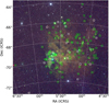 |
Fig. 1 Exposure-corrected three-colour image of the entire LMC observed by eROSITA during eRASS:4 in the colours red, 0.2–0.7 keV; green, 0.7–1.1 keV; and blue, 1.1–5.0 keV. The circles show the positions of confirmed SNRs while the squares show the position of SNR candidates. The green colour indicates that the sources were known in previous studies while in white colour we show the sources newly detected with eROSITA. |
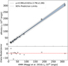 |
Fig. 2 Comparison between the luminosity measured with eROSITA and the luminosity reported in Maggi et al. (2016) based on data from XMM-Newton in the energy range 0.3–8.0 keV. The shaded region shows the 95% confidence interval around the best-fit line. The dashed line shows the 95% prediction interval. The bottom panel shows the residuals between the data and the best fit. From the plot, the agreement between the luminosities of SNRs obtained by the two different instruments is evident. |
3.5 Gaussian gradient magnitude filter
By visually inspecting the eROSITA LMC images we searched for new SNR candidates. To enhance the diffuse emission, we applied a Gaussian gradient magnitude (GGM) filter (Sanders et al. 2016) on the eRASS:4 images. The filter calculates the magnitude of the gradient of an image using Gaussian derivatives. Firstly, the input image is smoothed with a Gaussian filter of a certain σ. Secondly, the derivative along the x- and y-axis is taken. The magnitude of the gradient is then determined by summing the squared derivatives under the square root. Where the intensity of the image changes rapidly over the pixels the magnitude has a greater value, which can be used to highlight regions of rapid change in intensity. Usually, the edges of objects are characterised by such a change in intensity over pixels, which will be shown as maxima in the filtered image. Therefore, the GGM filter can act as an edge detection algorithm. The resulting image depends on the choice of σ for the GGM filter, which is measured in pixels. For a certain σ the filter will highlight the edges in the image with a certain pixel scale. Thus, we exploited various values of σ {σ = 1, 2, 4, 8, and 10 pixels) and combined the resulting filtered images into one. In order to reduce the noise resulting from point sources we applied the GGM on the point source subtracted count rate image.
We repeated the procedure described above for each energy band. The result of this technique is shown in Fig. 3. This image was useful to detect faint sources or, also to check if at the position of a known SNR candidate an edge structure is detectable. In Fig. 4 we show the effect of the GGM filter on a relatively bright, known SNR. The GGM filter highlights the edges of the emission. This technique was particularly useful in identifying SNR candidates in crowded regions. We point out that this procedure was used to find interesting region for further investigation. For the identification, the sources detected with the GGM filter were further investigated using the X-ray count rate image and images at other wavelengths as described in Sect. 4.
3.6 Hardness ratio
The faintness of many of the sources prevented us from performing a detailed spectral analysis for all sources. Therefore, we calculated the hardness ratios (HR) for all sources. We defined four energy bands: soft = 0.3–0.7 keV, medium = 0.7–1.1 keV, hard = 1.1–2.3 keV, harder = 2.3–4.0 keV and determined the net count rates in each energy band. We then computed three hardness ratios according to Eq. (1) for two adjacent energy bands:
 (1)
(1)
where EHRi is the error of each HRi (Sasaki et al. 2018). Ri is the net count rate in each energy band, ti is the average exposure time inside the emission region for each energy band, and eRi is the error of the net count rate calculated as  . The average exposure time was calculated using the exposure map obtained from the exmap task corrected for the vignetting effect.
We only included sources with a net count rate greater 0.01 cts s−1 in the energy band 0.2–5.0 keV. Among them, we selected the sources with a net count rate greater than 0.001 cts s−1 in each band (soft, medium, hard, and harder). We plotted HR1 versus HR2 and HR2 versus HR3 in Fig. 5 with SNR types from the classification proposed in Maggi et al. (2016). In the plot we also excluded the data points with an error larger than 0.5. The energy bands are chosen in a way that they will allow us to separate core-collapse (CC) SNRs and type Ia SNRs. For type Ia SNRs, we expect enhanced Fe-L emission between 0.7 and 1.1 keV. Therefore, HR1 is positive, while HR2 is negative. Core-collapse SNRs will also be brighter at higher energies, hence a positive HR2. As the sensitivity of eROSITA drops significantly above 2.3 keV, HR3 is unfortunately not so useful, which can also be seen in the large errors.
We also compared the HRs with predicted values assuming different typical spectral models. We assumed a thermal plasma in non-ionisation equilibrium (NEI) with different ionisation timescale τ and different temperatures. We used the model for variable abundance non-ionisation equilibrium (VNEI), which allows us to vary the element abundances, and assume an enhanced Fe abundance by setting Fe = 2 Z⊙ to simulate a type la SNR, while in the other case we assumed an enhanced O abundance (O = 2Z⊙ as the ejecta of CC SNRs is enriched with α-elements. In addition, we assumed a powerlaw spectrum with different photon indices Γ. These models take into account the hard sources in which there can be non-thermal emission from the shell in young SNRs or from a pulsar wind nebula.
The Fe-rich models tend to occupy more the lower right corner of the HR1–HR2 plot in Fig. 5, while the O-rich models tend to result in higher HR2. This trend is also visible in the distribution of the data points where we can clearly see a separation between type Ia (red squares) and CC (blue stars) SNRs. In the HR2–HR3 diagram, where the separation is much more difficult to see, we instead estimated the probability density function of the two distributions of the CC and type Ia SNRs using the python package gaussian_kde5, which allows us to better display the separation between CC and type Ia SNRs. We note that although SNRs with different progenitors seem to have different HRs, we could not determine the origin of the SNR by only considering the HRs. In this work, we discuss the possible progenitor type by combining the HRs with information about the underlying stellar population at the location of the SNR (see Sect. 5).
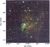 |
Fig. 3 eROSITA three-colour image after point sources were removed and the GGM filter was applied. This GGM-filtered image shows the magnitude of the gradient of the input image. The filter was applied to each energy band separately and the resulting images were combined into a three-colour image. |
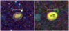 |
Fig. 4 Three-colour eROSITA image of SNR 10550-6823 (left) and with GGM filter applied. |
4 Multi-wavelength analysis
Supernova remnants are multi-wavelength objects and can be observed from radio to X-rays, in some cases also in gamma-rays. Morphologically, SNRs have mainly bubble- or shell-like structures and can easily be confused with H II regions and planetary nebulae (PNe). To find new SNRs, a multi-wavelength investigation is mandatory. The candidates were first identified in the eRASS:4 data by visually inspecting the count rate image and the GGM image (see Sect. 3). If there is X-ray emission with a surface brightness 1σ above the local X-ray background with a diffuse or shell-like emission, we classify the source as an SNR candidate. In addition, we also inspected the optical narrow-band images and the radio image. Only if we observe emission indicative of an SNR in at least one other band, either in optical or in radio, and the X-ray emission is at 3σ level, we confirm the source as an actual SNR.
In the optical, we looked for an excess in the ratio of two emission line fluxes [S IJ]/Hα. For [S II]/Hα < 0.4 the gas is photo-ionised, a process which typically occurs in HII regions around young and hot stars or in super-bubbles. For [S II]/Hα > 0.4 the ionisation is likely caused by a shock (Mathewson & Clarke 1973; Dodorico et al. 1980; Fesen 1984; Blair & Long 1997; Matonick & Fesen 1997; Dopita et al. 2010; Lee & Lee 2014; Vučetić et al. 2019b; Vučetić et al. 2019a; Lin et al. 2020). The presence of a shock wave is a strong indication for the presence of an SNR. In the radio band, the presence of an SNR is usually identified by measuring the spectral index α defined as Sv ∝ vα, where Sv is the flux density and v the frequency. for SNRs we expect α −0.5, which indicates non-thermal emission in the radio band (Filipović et al. 1998; Guzmán et al. 2011).
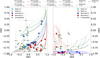 |
Fig. 5 Hardness ratios of candidates and confirmed SNRs in our sample. The energy bands used to calculate the hardness ratios are for HR1 : soft (= 0.3–0.7keV) and medium (0.7–1.1 keV), for HR2: medium (0.7–1.1 keV) and hard (1.1–2.3 keV), and for HR3: hard (1.1–2.3keV) and harder (2.3–4.0 keV). The sources are separated according to the explosion type as reported in Maggi et al. (2016). The SNRs tend to be separated according to the progenitor type of the remnant. The lines describe the expected HR values assuming different models. In particular we considered Fe-rich thermal plasma emission (VNEI with Fe = 2Z⊙) plotted with red lines and O-rich thermal plasma emission (VNEI with O = 2Z⊙) plotted with blue lines with different ionisation timescales τ (τ = 1010 s cm−3 and τ = 1012 s cm−3) and different temperatures (kT = 0.3 keV and kT = 0.5 keV). In addition, we also plotted power law models in green with different photon indices T (r = 1,2,3). The dashed and dotted black lines indicate different column densities NH = 0.0,0.5 and 1.0 cm−2. The contours in HR2-HR3 represent the Gaussian kernel-density estimation for core-collapse (CC) and type Ia SNRs. The contours indicate 68, 90, and 95% probability. |
4.1 Optical
To investigate the optical counterpart we used the MCELS data, which is very useful for studying the SNR as it provides us with narrow-band images of Hα, [S II], and [O III].
Essential for the detection and classification of SNRs is the ratio [S II]/Hα as described above. For [S II]/Ha higher than 0.4, ionisation and excitation of S is enhanced due to a radiative shock as suggested by several radiative shock models (Raymond 1979; Hartigan et al. 1987; Dopita & Sutherland 1995; Allen et al. 2008). However, several studies of SNRs and SNR candidates have shown that this separation can be less clear especially for sources with low surface brightness (see, e.g., Long et al. 2018, for a study of sources in M33). For this reason, in this work, we used [S II]/Hα > 0.67, which is a more reliable lower limit for identifying shock emission (Fesen et al. 1985). In addition, it is necessary that the emission of Hα is significant, as a low Hα flux might cause an artificial enhancement of the [S II]/Hα ratio. As pointed out also by Yew et al. (2021) the line ratio is an effective way to identify radiative SNRs, but it will miss the young non-radiative and Baimer-dominated SNRs (Chevalier et al. 1980).
4.2 Radio
From SNRs, we expect predominantly non-thermal emission in radio via synchrotron radiation. In young SNRs, synchrotron emission is also observed in the X-ray band. The more energetic electrons, emitting synchrotron radiation in X-rays, lose energy faster than the less energetic electrons, which will stay relativis-tic and emit in the radio band much longer. We used the public data from the ASKAP interferometer at 888 MHz (Pennock et al. 2021). The ASKAP LMC survey covers the entire LMC.
In order to highlight the non-thermal emission in the radio images we used the same approach as in Bozzetto et al. (2023) and in Ye et al. (1991). If there was no SN explosion inside an emission nebula we expect a correlation between the Hα emission and the radio continuum. This is due to the fact that the free electrons that produce thermal radio emission via Bremsstrahlung are the same as those that recombine with the protons to produce the Hα lines. We can use this proportionality to highlight the non-thermal emission in the radio images. After subtracting a scaled Hα image from the radio continuum what remains is just the non-thermal emission. In order to subtract the optical image from the radio image, we need a normalisation factor. This factor can be determined from the correlation between the pixel values in Hα and the radio continuum in regions where we expect that the emission is just thermal. In order to measure the correlation, we selected different H II regions in the entire LMC. We measured the [S II]/Ha ratio and selected only those emission nebulae with a ratio [S II]/Hα < 0.4 in order to make sure that there are no SNRs hidden inside the selected H II regions. We measured the intensity of Hα and radio continuum from the same region and compared the values. We performed a linear fit in the Hα-radio diagram and calculated the Pearson coefficient to evaluate the goodness of the fit. The slope of the plot is the normalisation factor, which can be used to normalise the Hα before subtracting it from the radio continuum. We averaged the different slopes using a weighted average using the Pearson coefficients as the weight.
In Fig. 6 we show the example of the H II region DEM-L140. Figure 6a shows the Hα emission, Fig. 6b shows the radio continuum of DEM-L140, and Fig. 6c shows the [S II]/Hα ratio. In order to avoid outliers, which could contaminate the linear fit we recursively cleaned the data until the standard deviation of the pixel value vector stopped to decrease. The linear relation and the linear fit are shown in Fig. 6d. We adopted the average slope as the normalisation factor for the Hα image and subtracted the scaled Hα emission from the radio-continuum emission. The H II regions used are: DEM-L111, DEM-L140, DEM-L194, DEM-L196,LHA-120-N44J, LHA-120-N70, MCELS-L401, N11, N44C, NGC-1899. From these H II regions, we selected several smaller regions and obtained a total of 61 sub-regions. To calculate the average slope we only kept the regions that show a Pearson coefficient greater than 0.9. Using this criterion we have a final number of 11 regions that contribute to the averaged slope. In Table 2 we report the selected H II sub-regions used to calculate the average slope with the relative fitted slopes and the Pearson coefficients for each sub-region. At the end of the table, we give the final average slope used to normalise the Hα emission. The error on the average slope was calculated using the formula to propagate the error on the weighted average:
 (2)
(2)
where wi are the Pearson coefficients and σi are the errors on the single fitted slope. The error on the single slope has been calculated using the python package used to fit the slope of the correlation scipy.optimize.curve_fit6.
After the subtraction of the scaled Hα from the radio continuum image only the non-thermal radio emission remains. We used it to draw contours in the radio continuum images at 3 and 5σ levels above the background to search for significant emission in an SNR.
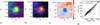 |
Fig. 6 Sub-region of the HII region DEM-L140 chosen to highlight the non-thermal emission in the radio images. In particular Figs. 6a and 6b show the emission of the selected region in Hα and radio respectively. Figure 6c displays the image of the [SII]/Hα ratio. The latter image is used to ensure that the selected region is not affected by any SNR that would increase the [SII]/Hα ratio to values larger than 0.4. In Fig. 6d the linear correlation between the Hα and radio emission in the selected area is reported. The black solid line represents the best linear fit for this correlation. |
H II regions used to calibrate the normalisation factor for the Hα images.
5 Star formation history-based progenitor classification
A necessary (but not sufficient) condition for a CC SNR is the presence of recent star formation activity near the SNR. In order to find the possible origin of SNRs and SNR candidates, we estimated the number of OB stars in the proximity of each source. We used the star formation history (SFH) values measured by Mazzi et al. (2021) using the near-infrared photometry from the VISTA survey of the Magellanic Clouds (VMC). The VMC data covers a sky area of ~96 deg2 and consists of infrared observations in the Y, J and Ks bands. Mazzi et al. (2021) calculated the SFH by comparing the synthetic Hess diagrams with the observed Hess diagram. A Hess diagram shows how many stars are located in a sub-region of a color-magnitude diagram (CMD). The CMDs, and therefore the Hess diagrams, can be constructed using different colours, in particular: Y – Ks versus Ks and J – Ks versus Ks, called YKs and JKs respectively in the figures showing the SFH for the eROSITA SNRs and SNR candidates (in Fig. 7 and Fig. E.2, available on Zenodo). The synthetic CMDs were calculated using a library of isochrones, which depend on the initial mass function (IMF), distance, extinction, binary fraction and SFH. A set of isochrones constitutes a model. In general, it is possible to independently measure the distance, extinction, and binary fraction and to assume an IMF. In this case, the best fit model can be used to calculate the SFH. For more details on the models see Mazzi et al. (2021), Harris & Zaritsky (2001), and references within.
We report the SFH around each source within a radius of 100 pc. This corresponds to the maximal projected distance that a star with a typical velocity of 10 km s−1 travels in 107 yr. For the eROSITA candidates and SNRs we plotted the SFH (see Fig. 7 and Fig. E.2, available on Zenodo). In Maggi et al. (2016) the authors calculated the number ratio of the two SNR types  . This number seems to be lower than the results of the local SN survey (Li et al. 2011) and the ratio derived from the abundance pattern of the intra-cluster medium chemically enriched by SNe (Sato et al. 2007) and indicates a higher relative number of type Ia SN in the LMC than in other galaxies. However, as discussed in Maggi et al. (2016), this lower NCC /NIa could be caused by observational bias, as some CC SNRs can be missed because they occured inside superbubbles. However, in our study we confirm the same tendency, as many of the newly confirmed SNRs and new candidates show indications to be thermonuclear SNRs.
6 Classifications of supernova remnants and candidates
As summarised in Sect. 3.1, the first step in the identification of the new candidates was the visual inspection of the eROSITA count rate image in three energy bands and the GGM filtered images. In order to understand if there is emission associated with an SNR, we compared the X-ray, optical and radio images (see Sect. 4). The images are shown in Figs. 7, 8a, and in Fig. E.2 (available on Zenodo). For each SNR or candidate, we show the three-colour eROSITA image of the source in the bands 0.2–0.7 keV, 0.7–1.1 keV, and 1.1–5.0 keV in the left image. The contours show the source surface brightness with 1σ, and 3σ above the local X-ray background. The second image is the GGM image of the X-ray emission, described in Sect. 3.5. The GGM was used in order to visually find possible region of interest, but it was not used to confirm any of the sources. The third panel shows the MCELS image, which shows the emission of Hα, [S II], and [O III]. The contours in the optical image represent regions with [S II]/Hα > 0.67. In the right panel, we show the radio continuum image from the ASKAP survey of the LMC at 888 MHz. The contours indicate non-thermal emission at 2σ, 3σ, and 5σ above the background as described in Sect. 4.2. For the first criterion to classify the source we used the X-ray contours. If at least 1σ emission (cyan contours in the eROSITA images) is detected we propose the source as a candidate. The classification of a source as a confirmed SNR requires a 3σ emission (red contours) in the X-ray image and, in addition, a confirmation in at least one other wavelength band (radio or optical): either the optical line ratio is [S II]/Hα > 0.67 or there is non-thermal emission in the ASKAP radio data. Optical or radio emissions, which satisfy these criteria are shown with red contours in the MCELS and ASKAP images. The most promising SNRs and candidates have been proposed and accepted for follow-up XMM-Newton observations. Section 6.1 presents three newly discovered and confirmed SNRs, Sect. 6.2 reports the confirmation of one previous candidate as an SNR, Sect. A presents 13 new candidates, Sect. B discusses the eROSITA data for 14 previously known SNRs, which were not in the catalogue of Maggi et al. (2016) and out of which two are not detected, and Sect. C presents 34 previous candidates, which are still not confirmed as SNRs after the eRASS:4 analysis. All confirmed (both previously known and newly confirmed in this work) SNRs in the LMC are listed in Table D.1 (available on VizieR).
6.1 Supernova remnants discovered and confirmed with eROSITA
The new SNRs first found in eROSITA and then confirmed thanks to the multiwavelength analysis are described below. The name of each source follows the convention for SNRs in the Magellanic Clouds (MC) while in brackets we report the name following the eROSITA convention. The newly found and confirmed SNRs with their X-ray properties obtained from eRASS:4 are listed in Table D.2 (available on VizieR).
MCSNR J0456–6533 (4eRASSU J045650.7-653244). The source is shown in Fig. 7 (upper left). This source was seen for the first time in the eROSITA data. There is a diffuse soft emission, while the emission is harder in the centre (with emission in the 0.7–1.1 keV band) and thus appears green in the three-colour image. Even though the 3σ detection is present just in a small portion of the source we confirm the source as an SNR thanks to the XMM-Newton follow-up observation described in Sect. 7. In the optical image, there is a shell-like structure in [O III] with a small enhancement of [S II]/Hα > 0.67 in the north of the shell. In the radio image, there is a very faint emission correlated with the optical shell, which surrounds the X-ray emission. We thus confirm the source as an SNR. We also show the plot of the SFH, in which there is an enhancement of star formation at around 109 yr ago. The recent SFR has a large uncertainty, which prevents us from arguing for a recent star formation activity. Combining the information from the spectral analysis, discussed in Sect. 7 and the SFH we suggest a type Ia origin for the remnant.
MCSNR J0506–7009 (4eRASSU J050615.8–700920). The source is shown in Fig. 7 (upper right). The source is located next to a molecular cloud known as LMC N J0506-7010 (Fukui et al. 2008). It has a relatively small size of 98″ × 72″. The source shows a peak of emission in the energy band of 0.7–1.1 keV. The image shows a clear 3σ detection. In the optical band, we can see a faint shell of [S II] and a strong enhancement of [S II]/Ha especially in the north-east. In the radio band, the continuum emission is very faint but with a non-thermal emission in the north-east, with the contours suggesting a semi-shell structure. We confidently confirm the source as a new SNR. The SFH shows a peak at around 109 yr ago, but also a lower peak at around 108 yr ago. The SFH does not show a particular activity in the recent past. The hardness ratios HR1 = 0.68 ± 0.11 and HR2 = −0.68 ± 0.08 suggest that the source is located in the region populated by type Ia source in the HR1 – HR2 diagram. Combining the HRs, the colour of the image, and the SFH we suggest a thermonuclear progenitor for the SNR.
MCSNR J0543–6624 (4eRASSU J054348.6–662351). The source is shown in Fig. 7 (bottom). The source shows a diffuse soft X-ray emission with an irregular rectangular shape and has a 3σ emission in the centre. In the optical band, we can see a rectangular shape similar to X-rays embedded in a H II region with an enhancement of the ratio [S II]/Hα. In radio, there is also a faint rectangular shell in agreement with the optical shell; however, we did not detect any clear non-thermal emission. The SFH peaks at 107 years ago, which suggests a possible CC origin for the remnant. Also in the HR diagrams, the source is in the region typical for CC SNRs. The CC origin is also in agreement with the fact that the source is embedded in a H II region. Combining the X-ray and the optical information we confirm the source as an SNR.
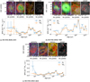 |
Fig. 7 For each source, the eROSITA count rate three-colour image (left) with red: 0.2–0.7keV, green: 0.7–1.1 keV, and blue: 1.1–5.0keV; the GGM filter image (see Sect. 3.5) applied to the eROSITA count rate (middle left); the MCELS survey three-colour image (middle right) with red: Hα, green: [S II], and blue: [O III]; and the ASKAP radio continuum image (right) in the upper panel. The white circles (ellipses) show the extraction region for determining the count rates (see Sect. 3.3). The cyan (red) contours in the eROSITA three-colour image show the detection at 1σ (3σ) over the background in the energy band 0.2–1.1 keV. The contours in the optical image represent [S II]/Hα > 0.67. The contours in the radio image show the non-thermal emission calculated as described in Sect. 4.2. In the lower panel we show the SFH as calculated in Mazzi et al. (2021) using J – Ks and Y – Ks (see Sect. 5). |
6.2 Previous MCELS candidate confirmed with eROSITA
MCSNR J0454–7003. The source is shown in Fig.E.1 (available on Zenodo) and the X-ray property reported in Table D.3 (available on VizieR). This source was proposed by Yew et al. (2021) as an optical SNR candidate. It is located on the south-east edge of the H II region LHA 120-N 185 overlapping half with the H II region (Davies et al. 1976; Pellegrini et al. 2012). In the optical band, the candidate shows a circular structure where the emission is dominated by [S II] and Hα. The ratio [S II]/Hα is > 0.67 in the southern part of the shell and where the source coincides with the H II region. In the radio image, there is diffuse emission at the position. However, there is no significant detection. In X-rays, there is diffuse emission in the H II region and 3σ emission at the position of the optical SNR candidate. As this source fulfils the optical ([S II]/Hα > 0.67) and X-ray (3σ detection) criteria we confirm this source as an SNR.
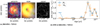 |
Fig. 8 Multiwavelength view of J061438.1-725112 and SFH in the nearby 100 pc. (a) eROSITA count rate three-colour image of J061438.1-725112 (left) with red: 0.2-0.7keV, green: 0.7-1.1 keV, and blue: 1.1-5.0keV, the GGM filter image (see Sect. 3.5) applied to the eROSITA count rate (middle left), and the ASKAP radio continuum (right). The white circle shows the extraction region for determining the count rates (see Sect. 3.3) The cyan (red) contours in the eROSITA three-colour image show the detection at 1σ (3σ) over the background in the energy band 0.2-1.1 keV. The contours in the optical image represent [S II]/Hα > 0.67. The contours in the radio image show the non-thermal emission calculated as described in Sect. 4.2. The (b) panel shows the SFH as measured in Mazzi et al. (2021) using J – Ks and Y – Ks (see Sect. 5). |
6.3 Supernova remnant candidates detected with eROSITA
In the eROSITA data, we detected 16 new diffuse sources in the X-ray images. Among them, we are able to confirm three as SNRs as presented in Sect. 6.1. We present the 13 new SNR candidates detected with eROSITA for the first time in Appendix A. Among the new eROSITA candidates, we emphasize the peculiarity of 4eRASSU J061438.1–725112 (J0614–7251) described in the following section. This source is the first X-ray SNR candidate detected in the outskirts of the LMC. The X-ray properties are reported in Table D.4 (available on VizieR), while the images are shown in Fig. E.2 (available on Zenodo).
4eRASSU J061438.1–725112 (J0614–7251). The source is shown in Fig. 8a. This source is of particular interest as it is not located in the LMC but far out in the south-east, also outside of the Magellanic Bridge (MB). The source was discovered in the eROSITA images because of its relatively bright appearance with an approximately spherical shape. The region is not covered by the MCELS survey, therefore we do not have any optical data. The region was covered in the ASKAP survey of the LMC, but it is on the edge of the image where the radio sensitivity is lower and did not allow us to detect anything in the radio band. In X-rays, the source has a shell-like structure in the soft X-rays in the east. The inner part appears slightly harder with an orange colour. The source shows a prominent emission above the 3σ level. The net count rate is (2.76 ± 0.12) × 10−1 counts s−1. As there is no optical or radio confirmation, this source is an SNR candidate. In the SFH in Fig. 8b there are no recent peaks in star formation, therefore, ruling out the CC origin for this SNR candidate. The circular shape also suggests that the source could have originated from a Type Ia SN (Lopez et al. 2009, 2011). Interestingly, the HR diagram suggests that the source might be related to a CC SN. Further investigations are needed to confirm or rule out the SNR nature of this source and, in the former case, to correctly classify the origin of the SNR candidate. We stress the peculiarity of the spatial location of the source. If this source is confirmed to be an SNR, it will be the first SNR detected outside a galaxy in the Magellanic System. The lack of multi-wavelength information did not allow us to confirm the source as an SNR, but it remains a very promising SNR candidate.
6.4 Known supernova remnants not included in Maggi et al. (2016) but observed with eROSITA
The catalogue of Maggi et al. (2016) contains 51 confirmed SNRs. Here we summarise the SNRs, which were confirmed in later studies. The multiwavelength description of these sources is given in Appendix B. The eROSITA X-ray properties are reported in Table D.5 (available on VizieR). The images are shown in Fig. E.3 (available on Zenodo).
6.5 Previous candidates that remain candidates
In Appendix C we describe the previously known candidates, which could not be confirmed using the eROSITA data. The respective X-ray properties are listed in Table D.6 (available on VizieR) and the images are shown in Fig. E.4 (available on Zenodo).
7 XMM-Newton observations of MCSNR J0456–6533
The source was detected for the first time in the eROSITA survey and proposed for an XMM-Newton follow-up observation. The original exposure time was ~45.0 ks, while after the flare removal, the exposure time was reduced to 33.7 ks. Figure 7 shows the eROSITA X-ray image and the comparison with emission at other wavelengths. As described in Sect. 6.1, in the optical there is a shell in [O III]. In the radio continuum, there is also a very faint shell that coincides with the shell in the optical. In the X-ray three-colour image the SNR has a green central region, suggesting a peak in the emission around 1.0 keV, which is typically due to the presence of Fe L lines and characteristic for a type Ia SN. The remnant also presents a softer ring in the outer region, which is mainly visible in the east. The colours suggest that we are observing ejecta that have been heated by the reverse shock. Figure 9 shows the XMM-Newton three-colour image in which the same structures as in the eROSITA image are visible. From the radius of the remnant (~37pc), assuming an pre-explosion number density of 0.1 cm−3 and an explosion energy of 1051 erg we estimate the age to ~42 [(E/1051 erg)/(n/0.1 cm−3]−1/2 kyr, assuming a Sedov expansion (Borkowski et al. 2001).
We performed a spectral analysis of the source using the XMM-Newton data. We chose an interior circular region covering the emission appearing in green in the three-colour image around ~ 1 keV, an outer annulus covering the soft shell, and a circle covering the entire source (white circles in Fig. 9). In particular, we are interested in understanding the origin of the different colours in the X-ray three-colour image between the inner and outer regions. The spectrum of an additional background region is taken from a ring around the source (green annulus in Fig. 9).
We used XSPEC (version 12.13.0 c) and AtomDB (version 3.0.9) to analyse the spectra. We performed a combined fit using data from EPIC-pn, -MOS1, and -MOS2 cameras. To model the background we used different contributions (Snowden et al. 2008): the Local hot bubble (LHB) emission modelled as a non-absorbed thermal plasma with a rather low temperature of kT = 0.1 keV, the Galactic halo modelled as two absorbed thermal components and an extragalactic component caused by the unresolved AGN in the background modelled by a power law.
For the thermal components of the background, we used the APEC model for thermal plasma in collisional ionisation equilibrium (Smith et al. 2001). For the LHB, the temperature is fixed to kT = 0.1 keV. The Galactic halo emission consists of a ‘hot’ component with a typical temperature of kT = 0.3–0.8 keV and a ‘cold’ component with kT = 0.1–0.3 keV. For the absorption of the halo emission, the Galactic column density in the direction of the source was assumed (Dickey & Lockman 1990). For the emission of the unresolved extragalactic background, we used an absorbed power-law model with a fixed photon index of Γ = 1.46 (Lumb et al. 2002; De Luca & Molendi 2004; Moretti et al. 2009). This component is absorbed not only by the Galactic absorption but also by the material inside the LMC. Therefore, an additional absorption component was included and allowed to vary during the fit. The normalisation of all the components was free to vary during the fit. We also considered Solar wind charge exchange (SWCX), which can have an important contribution at low energies and was modelled with six Gaussian functions with a line width of zero. The SWCX lines modelled are the following: C VI (0.46 keV), O VII (0.57keV), O VIII (0.65 keV), O VIII (0.81 keV), Ne IX (O.92keV), Ne IX (1.02 keV) and Mg VI (1.35 keV) (Snowden et al. 2004).
The particle background was modelled assuming a power law. Since the particle background does not interact with the mirrors of the telescope, the power law was not folded with the ancillary response file (ARF) of the instrument. The fit of the background spectrum yielded Γ = 0.15.
To take the instrumental background into account, we added Gaussian lines for the instrumental lines Al Kα at 1.48 keV and Si Kα at 1.75 keV for EPIC-MOS1/MOS2. For EPIC-pn the Al Kα line as well as four additional lines at 7.49, 8.05, 8.62, and 8.90 keV need to be considered.
For the fit of the source spectrum, the local X-ray background was not subtracted, but all background spectrum components were included in the model. The parameters of the background spectrum were fixed to the best-fit values, and the background spectrum was scaled by the ratio of the areas in the source and background regions. For the source emission, we used one absorbed NEI plasma model with variable element abundances VNEI. The Galactic column density towards the source was frozen to the value measured by Dickey & Lockman (1990), while we included an additional absorption component for the LMC with the average LMC abundances of 0.5 times the solar value (Westerlund 1997). This absorption column density was a free parameter during the fit. We used the same model for all source extraction regions. First, we froze all the abundances in the emission component to 0.5. In the inner, outer, and entire regions, the fitted absorption in the LMC is very low (NH < 0.07 × 1022 cm−2) and is not constrained as shown in Fig. 10. We get an upper limit of 0.07 × 1022 cm−2 at the 90% confidence level. Additionally, no difference in the LMC absorption between the outer and the inner regions is observed. We conclude that the source is not significantly absorbed by material in the LMC. Spectra are shown in Fig. 11.
The ionisation timescale τ for the inner region is >1013 s cm−3, which indicates that the plasma is in ionisation equilibrium. By contrast, for the outer part, we have two statistically equivalent models: the first one presents a low temperature (~0.12keV) and a large τ (~1013 s cm−3), whereas the second model suggests a low t (~1010 s cm−3) and a higher temperature (~0.33 keV). The low counts of the outer region prevent us from constraining the best-fit model with enough statistical significance. With a measured radius of ~37 kpc (assuming a distance of 50 kpc), the SNR is rather evolved and the forward shock has decelerated significantly. Therefore, it is likely that the shock temperature is low and the shocked ISM is close to ionisation equilibrium (high τ). We point out that in the outer region, we observe most of the emission in the East, while in the West the outer emission is particularly faint. This could be due to a gradient in the density of the ISM surrounding the SNR (the X-ray emission depends on the density squared). Assuming that the outer ring emission is from the shocked ISM we fit the VNEI component for the source emission with all the abundances frozen to 0.5 Z⊙. The best-fit temperature is lower than the temperature measured in the inner region. We conclude that the softer emission in the outer region is due to the lower temperature of the shocked ISM. In general, the temperature in the inner part is higher than the temperature measured in the outer part. The fitted temperatures are reported in Table 3. The uncertainties of all parameters listed were calculated using the XSPEC command steppar within a confidence interval of 90%.
The green colour of the inner part is probably due to a combination of a higher temperature plasma with respect to the outer part, and a difference in elemental abundances. To investigate this possibility we let the Fe abundances free to vary for all regions. The fit results in a high Fe abundance for the inner region (see Table 3). We also tried to fit the Fe abundance in the outer region, but it was not constrained, probably due to the lack of photon statistics.
In the inner part, we observe an enhancement of Fe abundance. Despite this fact, the Fe abundance and the temperature tend to be slightly degenerate (see Fig. 10). We observe that the Fe value is always higher than 0.5 Z⊙, indicating that the green colour in the inner region is most likely due to Fe emission of the ejecta. This suggests that the ejecta have been heated by a reverse shock that occurred in the past. In addition, the high abundance of Fe suggests that the SNR has a type Ia SN origin. Figure 11 shows the spectra of the inner and outer regions. In order to compare the XMM-Newton and eROSITA observations we calculated the luminosity using the best-fit model for the entire region of the remnant obtained by fitting the same model to the XMM-Newton and the eROSITA data. Also for the entire remnant we obtain a high τ value (~1013 s cm−3) and low foreground absorption. The fitted temperature is (~0.22 keV), which is between the hot temperature of the inner part and the cold temperature of the outer ring (see Table 3). Because the eROSITA spectrum has fewer counts, we are not able to model the emission of the entire remnant with two separate VNEI components for the outer shell and the inner part. For this reason, we compared the eROSITA and spacially integrated XMM-Newton data by fitting each with a single VNEI component where all abundances were set to 0.5 Z⊙. This is justified as the emission of the outer shell dominates the emission of the remnant. Due to the lack of statistic we used the cstat implemented in Xspec and we used the ungrouped spectra. Also with eROSITA the best fit temperature for the entire remnant is (~0.22 keV) and and the foreground absorption is low (see Table 3). The ionisation timescale is not constrained and indicates ionisation equilibrium of the plasma (τ~1013 s cm−3). For consistency, we compare the luminosity determined with XMM-Newton and with eROSITA. We calculated the absorbed flux using the flux command in XSPEC removing the contribution from the background. We assumed a distance of 50 kpc (de Grijs et al. 2014) and convert the resulting flux to luminosity. The value of the luminosity for the XMM-Newton data is averaged over all three detectors EPIC-MOS1, MOS2, and pn and over TM 12346 for eROSITA. The uncertainties were calculated using Markov Chain Monte Carlo (MCMC) for the best-fit model. For XMM-Newton we find the luminosity to be  while the eROSITA luminosity is
  erg s−1 both in the energy band 0.3–8.0keV. Both uncertainties correspond to 90% confidence intervals. The possible inconsistency might be caused by the lower spatial resolution of eROSITA combined with the low photon statistics for the SNR, which makes it difficult to define the source region and the difficult estimation of the local X-ray background in particular with XMM-Newton.
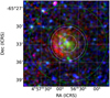 |
Fig. 9 Three-colour image of J0456–6533 with red for 0.3–0.7 keV. green for 0.7–1.1 keV, and blue for 1.1–4.5 keV. The inner white circle and the white annulus around it mark the two source extraction regions. The green annular region around the SNR shows the background extraction region. |
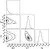 |
Fig. 10 Contour plots for the fitted parameters in the inner region of the remnant. The plotted contours are at 1, 2, and 3σ. From the contours, we measure the enhancement of Fe, which is always larger than 0.5 Z⊙ (i.e. the average abundance of ISM elements in the LMC). |
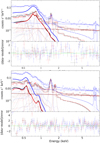 |
Fig. 11 XMM-Newton EPIC spectra of the inner circular region (top) and outer shell (bottom) of SNR J0456–6533. We plot the source spectrum (MOS1: black, MOS2: red, pn: blue) and the best-fit models. The thick solid lines show the contribution of the VNEI source emission component, which represents the emission of the SNR. All additional lines represent various background components as described in Sect. 7. |
Fit values for the XMM-Newton observation of MCSNR J0456–6533.
8 Conclusions
We have investigated the SNR population in the LMC using the SRG/eROSITA data, which provides a complete look at the LMC in the soft-to-medium X-ray band. The large field of view of eROSITA and the full coverage in eRASS:4 allowed us to study known SNRs and candidates and to find new SNRs and candidates. In general, we used X-ray 1σ detection to identify new SNR candidates. We compared the [S II]/Hα line ratios and the non-thermal radio emission to investigate the true nature of the source. The confirmation of a new SNR required at least two of the following criteria: 3σ detection in X-ray, [S II]/Hα > 0.67, and a non-thermal radio diffuse emission. The main results of this work are as follows:
We used the above-described multi-wavelength analysis to confirm three of the eROSITA candidates as SNRs (see Sect. 6.1).
Using a 3σ threshold for the X-ray emission, we were able to confirm one previously known candidate as an SNR: MCSNR J0454–7003 (see Sect. 6.2).
We performed a Gaussian gradient magnitude filter analysis on the eRASS:4 images of the LMC to identify possible new SNR candidates. Based on combining the X-ray data with optical and radio data, we propose 13 sources as new X-ray SNR candidates (see Sect. A). Using the HRs and the SFH around each source, we investigated the origin of these SNR candidates.
We propose J0614–7251 as the first X-ray SNR candidate in the outskirts of the LMC (see Sect. 6.3). The source presents X-ray emission above the 3σ level with a net count rate of (2.76 ± 0.12) × 10−1 cts s−1, resulting in a prominent isolated source. From the SFH, we cannot rule out a CC origin for this SNR candidate.
The results summarised in points 1–4 bring the total number of SNRs in the LMC to 77 and the number of SNR candidates to 47 (see Table 1).
We performed a spectral analysis of the newly detected MCSNR J0456–6533 using XMM-Newton data from a follow-up observation of the eROSITA detection (see Sect. 9). We modelled the source emission with a single absorbed VNEI model component and investigated different regions of the source. The column density in the LMC is very low (NH < 0.07 × 1022 cm−2), which suggests an unabsorbed source. We did not observe a significant difference in the fitted temperature between the inner part and the outer shell of the remnant. We found an enhancement in Fe abundance in the inner part, which is most likely dominated by ejecta emission, and it suggests a type Ia SN as the progenitor of MCSNR J0456–6533.
With this work we provide the most up-to-date catalogue of SNRs in the LMC. The large field of view and the high sensitivity in the soft X-ray band of eROSITA have allowed us to study SNRs and SNR candidates distributed over the entire LMC and its surroundings, making the population of SNRs in the LMC more complete and making the population study more robust. The discovery of SNR candidates in the LMC outskirts opens the possibility of investigating the evolution of SNRs in an intergalactic environment for the first time.
Data availability
The X-ray properties of the sources described in the paper are publicly available as Tables D.1-D.6, which are available in electronic form at the CDS via anonymous ftp to cdsarc.cds.unistra.fr (130.79.128.5) or via https://cdsarc.cds.unistra.fr/viz-bin/cat/J/A+A/692/A237. The images of the sources (E.1 - E.4) described in Appendices A, B, and C are available on Zenodo https://zenodo.org/records/13951085.
Acknowledgements
This work was supported by the Deutsche Forschungsgemeinschaft through the project SA 2131/14-1. M.S. and J.K. acknowledge support from the Deutsche Forschungsgemeinschaft through the grants SA 2131/13-1 and SA 2131/15-1. P.J.K. acknowledges support from the Science Foundation Ireland/Irish Research Council Pathway programme under Grant Number 21/PATH-S/9360. The paper is based on data from eROSITA, the soft X-ray instrument aboard SRG, a joint Russian-German science mission supported by the Russian Space Agency (Roskosmos), in the interests of the Russian Academy of Sciences represented by its Space Research Institute (IKI), and the Deutsches Zentrum für Luft- und Raumfahrt (DLR). The SRG spacecraft was built by Lav-ochkin Association (NPOL) and its subcontractors and is operated by NPOL with support from the Max-Planck Institute for Extraterrestrial Physics (MPE). The development and construction of the eROSITA X-ray instrument were led by MPE, with contributions from the Dr. Karl Remeis Observatory Bamberg, the Erlangen Center for Astroparticle Physics (ECAP), the University of Hamburg Observatory, the Leibniz Institute for Astrophysics Potsdam (AIP), and the Institute for Astronomy and Astrophysics of the University of Tübingen, with the support of DLR and the Max Planck Society. The Argelander Institute for Astronomy of the University of Bonn and the Ludwig Maximilians Universität Munich also participated in the science preparation for eROSITA. The eROSITA data shown here were processed using the eSASS/NRTA software system developed by the German eROSITA consortium. Part of this work was supported by the German Deutsche Forschungsgemeinschaft, DFG project number Ts 17/2–1. This work uses observations obtained with XMM-Newton – an ESA science mission with instruments and contributions directly funded by ESA Member States and NASA. In this paper we used data from ASKAP, The Australian SKA Pathfinder is part of the Australia Telescope National Facility, which is managed by CSIRO. Operation of ASKAP is funded by the Australian Government with support from the National Collaborative Research Infrastructure Strategy. ASKAP uses the resources of the Pawsey Supercomputing Centre. The establishment of ASKAP, the Murchison Radio-astronomy Observatory and the Pawsey Supercomputing Centre are initiatives of the Australian Government, with support from the Government of Western Australia and the Science and Industry Endowment Fund. We acknowledge the Wajarri Yamatji people as the traditional owners of the Observatory site. This work makes use of MCELS. The MCELS was funded through the support of the Dean B. McLaughlin fund at the University of Michigan and through NSF grant 9540747. This research has made use of Aladin, SIMBAD and VizieR, operated at the CDS, Strasbourg, France.
Appendix A Supernova remnant candidates detected with eROSITA
In the eROSITA data, we detected 16 new diffuse sources in the X-ray images. Among them, we are able to confirm three as SNRs as presented in Sect. 6.1. In the following section we present the 13 new SNR candidates detected with eROSITA for the first time. As these sources are not confirmed as SNRs, we first report the name following the eROSITA convention and in bracket the name as usually used in the SNRs catalogues. The list of the eROSITA candidates is reported in Table D.4 (available on VizieR) and the images in Fig. E.2 (available on ).
4eRASSU J045145.7–671724 (J0451–6717): The source is shown in Fig. E.2 (a). This candidate SNR might be associated with a radio pulsar detected by Manchester et al. (2006) using the Parkes radio telescope. The properties of the radio pulsar, including its position, are still highly uncertain. In our radio images, there is a point source inside J0451–6717, which can be associated with the pulsar, but further observations to measure the pulse period are required for confirmation. In the optical, there is an elongated shell structure particularly visible in [S II], where the [S II]/Hα ratio is partially higher than 0.67. In the X-ray images, there is faint diffuse emission, which correlates with the optical emission, however, only with a 1σ detection. Only very small portions of the remnant are detected with 3σ confidence. In the GGM image, we can clearly see an edge with an elliptical shape associated with the source. The region was observed with XMM-Newton but the candidate is located at the rim of the field of view, which prevented a previous detection. Since the 3σ detection in the eROSITA data is in a very small portion we conservatively keep the source as an SNR candidate. Recently, this source was accepted for an XMM-Newton follow-up observation. With a deeper observation, we will be able to further constrain the true nature of this source.
4eRASSU J045625.5–683052 (J0456–6830): The source is shown in Fig. E.2 (b). This source was identified for the first time in the eROSITA survey. In the X-ray three-colour image it is seen as a diffuse green emission, which means that the emission peaks at around 1.0 keV. Even if the source is relatively faint with a net count rate of (2.90 ± 0.78) × 10−2 cts s−1, it is clearly visible in X-rays. The brightest part is on the south-east, as the 1σ contour shows. The source is relatively compact with a diameter of about 160″ and has a circular shape. Also, the GGM image shows the presence of a diffuse emission. In the optical band, there is no compact emission clearly related to the candidate, but it is surrounded by a larger structure dominated by [S II]. The optical line ratio [S II]/Hα < 0.67 does not indicate shock emission. Neither in the radio continuum nor in the non-thermal component any emission is detectable. Therefore, the source remains a candidate. The SFH within 100 pc around the centre of the candidate indicates a relatively high and constant star formation activity from 109 to 108 yr ago. The HRs and the colour of the image suggest a possible thermonuclear origin.
4eRASSU J050750.8–714241 (J0507–7143): The source is shown in Fig. E.2 (c). From its green colour in the three-colour image, we can conclude that the peak of the emission is at around 1.0 keV. The presence of a diffuse source is confirmed by the GGM image. The source is relatively faint in the X-ray band with a count rate of (5.60 ± 1.41) × 10−2 cts s−1. We do not confirm any emission in the optical or in radio. In the radio image, there is a non-thermal source in the north that is an AGN in the background. The same AGN is visible as a point source in the X-ray image. We propose this X-ray source as an SNR candidate. The SFH around the source position has a peak between 109 and 1010 yr ago. The region around the candidate did not face a recent star formation activity. From the X-ray colour of the source and the SFH, we can argue for a type Ia origin.
4eRASSU J051028.3–685329 (J0510–6853): The source is shown in Fig. E.2 (d). This source is located next to a molecular cloud [WHO2011] C173 (Wong et al. 2011). There is a faint X-ray source, which is also clearly seen in the GGM image. In the optical band, there is a shell structure in the east. However, the radio [S II]/Hα is below the limit of 0.67, characteristic of an SNR. The radio image shows a shell structure on the east with a 3σ non-thermal emission, with a possible shell in the west. The SFH shows no recent star formation. The hardness ratios HR1 = −0.29 ± 0.15 and HR2 = −0.70 ± 0.33 correspond to values characteristic of CC SNR (see Fig. 5). Therefore, despite the SFH, we cannot rule out the CC scenario. Since there is a non-thermal shell-like source in radio but no X-ray is detected at the 3σ level, the source is classified as a candidate.
4eRASSU J052136.6–670741 (J0521–6707): The source is shown in Fig. E.2 (e). In the eROSITA image, there is a very faint diffuse source with a net count rate of (3.10 ± 1.37) × 10−2 cts s−1, confirmed by the GGM image. In the optical image, these is an enhancement of [S II]/Hα > 0.67 inside the shell. In the radio image, there is a point source detected by Filipovic et al. (1995) with the catalogue name B0521–6710 at 4.75 GHz, and by Marx et al. (1997) with the name MDM 15 and detected at 2.4 GHz. In the latter paper, they measure a spectral index of –0.3. No diffuse emission can be observed in the radio images. The SFH around the source indicates two relative peaks between 107 and 108 years ago. The absence of the 3σ detection in X-rays prevents us from confirming the source as an SNR, and it is classified as a candidate.
4eRASSU J052126.5–685245 (J0521–6853): The source is shown in Fig. E.2 (f). The source was detected in the ROSAT survey (Haberl & Pietsch 1999). In the eROSITA image, it is visible at 1σ level despite the source being located in a relatively bright environment. The GGM image shows an enhancement of the emission relative to the surroundings. At the same location, there is a diffuse emission in the optical image with Hα, [S II], and [O III] emission. There is a small bright region in the centre with a diameter of about 21″, embedded in a larger structure. There is no optical emission with [S II]/Hα > 0.67 at the position of the X-ray emission. However, it is [S II]/Hα > 0.67 in the surroundings. In the radio band, there is non-thermal emission north of the X-ray emission, wherein the optical the ratio [S II]/Hα > 0.67. The SFH around the source shows no recent star formation activity. The absence of the 3σ detection prevents us from confirming the source as an SNR, and it is classified as a candidate.
4eRASSU J052148.7–693649 (J0521–6936): The source is shown in Fig. E.2 (g). The source was identified for the first time with eROSITA probably because it is located in a region where the surrounding is bright in X-rays. There is a diffuse source in X-rays, which is clearly visible in particular in the GGM image. The emission is brighter in the north. It peaks at around 1 keV as the green colour suggests. There is a very small region with 3σ emission in the northern part. In the optical image, the source is surrounded by diffuse emission in the east and the south with only small regions with [S II]/Hα > 0.67. The X-ray peak correlates with a bubble-like structure in optical. In the radio image, we cannot see any structure that can be related to the X-ray source. The SFH indicates two relatively recent peaks around 4 × 10⁷ yr and 107 yr ago. The low significance of the detection in the X-ray band prevents us from confirming the source as an SNR, and classifying it as a candidate.
4eRASSU J052330.7–680400 (J0523–6804): The source is shown in Fig. E.2 (h). The X-ray images show a circular object with a radius of 116″. The GGM also shows the circular edge of the source. We do not observe any emission in the optical band. In the radio image, there is non-thermal emission, especially in the south. Unfortunately, there is no 3σ detection in X-rays. The hardness ratios HR1 = 0.04 ± 0.21 and HR2 = −0.89 ± 0.32 locate the source in the region in the HR1–HR2 diagram (Fig. 5) populated by thermonuclear SNRs. The green colour in the X-ray image shows a peak in the emission around 1 keV typical of thermonuclear origin. The SFH around the source has a peak in the recent past around 106 yr. This star formation activity would be compatible with a possible CC origin but from the position of the source in the HR diagram 5 and from the colour we propose the candidate to originate from an SN Ia. The absence of a 3σ detection in the X-ray image prevents us from confirming the source as an SNR. For this reason, we propose this source as an SNR candidate.
4eRASSU J052502.7–662125 (J0525–6621): The source is shown in Fig. E.2 (i). The source has an irregular shape in the X-ray images, with a softer emission in the north-east. There is some 3σ emission inside the source, but its distribution is not sufficient to confirm the source as an SNR. In the GGM image, we can observe a clearly enhanced edge. In the optical image, there is a strong enhancement of [S II]/Hα > 0.67 while in the radio image, there is a complex environment where the emission appears to be non-thermal. There is no structure in the radio emission that correlates with the X-ray or the optical emission. The HRs of the source indicate a type Ia SNR (see Fig. 5). There was quite constant star formation activity from 109 until today with a relative peak in SFH between 108 and 107 yr ago. We propose this source as a candidate.
4eRASSU J052849.7–671913 (J0528–6719): The source is shown in Fig.E.2 (j). The source is detected at 1σ level with a soft diffuse emission between 0.2 and 0.7 keV and thus appears red in the eROSITA images. In X-rays, it has a half-shell structure in the south, which is also visible in the GGM image. There is no emission that can be related to the X-ray source, neither in the optical nor in the radio. The SFH has a recent peak, which might suggest a CC origin.
4eRASSU J053224.5–655411 (J0532–6554): The source is shown in Fig. E.2 (k). The source was detected in the ROSAT data by Haberl & Pietsch (1999). Its ROSAT HRs suggested that it could be an AGN, SNR, or an X-ray binary. In the eROSITA images the source shows a diffuse emission with a count rate of (3.80 ± 0.50) × 10−2 counts s−1 and HR1 = 0.37 ± 0.12, HR2 = −0.65 ± 0.14. The contours in the X-ray image show a 3σ emission. No particular structure can be observed in the optical or radio image. For this reason, we propose the source to be a candidate. The SFH shows a recent increase in the star formation activity, which is nevertheless not significant enough to suggest a CC origin.
4eRASSU J054949.7–700145 (J0549–7001): The source is shown in Fig. E.2 (l). This source has an elongated shape in the north-east, south-west direction with a brighter emission in the south-west. The source is relatively bright with count rates of (5.80 ± 0.82) × 10−2 counts s−1. The 1σ contours follow the diffuse structure and small portions inside have detection with significance above 3σ. In the optical band, the region presents a complex filamentary emission, where it is not clear if any structure can be related to the candidate. No enhanced ratio of [S II]/Hα > 0.67 is observed. In radio, there is no emission associated with the source either. Therefore, this source is an SNR candidate. The SFH shows a small peak at around 5 × 10⁶ yr ago. However, its X-ray colour is indicative of a thermonuclear origin.
Appendix B Known supernova remnants not included in Maggi et al. (2016) but observed with eROSITA
The catalogue of Maggi et al. (2016) contains 51 confirmed SNRs. Here we summarise the SNRs, which were confirmed in works performed later. The eROSITA X-ray properties of the following SNRs are reported in Table D.5 (available on VizieR), while the images are shown in Fig. E.3 (available on Zenodo).
MCSNR J0447–6918: The source is shown in Fig. E.3 (a). The source is confirmed by Kavanagh et al. (2022) using XMM-Newton data. The source was a radio candidate proposed by Bozzetto et al. (2017). The remnant presents a diffuse emission in the radio continuum. We detect non-thermal emissions, especially coming from the centre of the source. In the optical band, we can observe a half-ring structure in the south with high [S II]/Hα. There is some additional filamentary emission that extends from the inner part of the shell to the north-east. The optical emission correlates with the diffuse radio emission. In X-rays, we also detect an elongated faint emission, which is more visible using the GGM filter and it agrees with the shell seen in the optical and radio images.
MCSNR J0449–6903: The source is shown in Fig. E.3 (b). This source was another radio candidate proposed by Bozzetto et al. (2017) and confirmed by Kavanagh et al. (2022). In radio, the source presents a prominent diffuse emission. The remnant shows that there is a strong non-thermal emission that correlates with the entire diffuse emission. In the optical, there is a faint shell of [O III], where the interior has an enhancement of [S II]/Hα. Neither in the eROSITA images nor in the GGM image we can detect any significant emission.
MCSNR J0456–6950: The source is shown in Fig. E.3 (c). This was another radio candidate (Bozzetto et al. 2017) confirmed as an SNR by Kavanagh et al. (2022). The radio image presents a diffuse spherical emission with the presence of non-thermal emission in the entire remnant. Neither in the eROSITA images nor in the optical images, any clear emission can be associated with the remnant.
MCSNR J0504–6723: The source is shown in Fig. E.3 (d). This remnant was proposed as an X-ray candidate by Haberl & Pietsch (1999) and confirmed by Kavanagh et al. (2022). Also in the eROSITA images the source appears as a bright diffuse emission with a peak at around 1.0 keV. In radio we do not detect any non-thermal emission and the continuum does not show a structure that can be connected to the remnant. In the optical image, we can clearly see an enhancement of the [S II]/Hα ratio, especially in the north. In the rest of the region, we can see filaments of Hα and [SII].
MCSNR J0506–6815: The source is shown in Fig.E.3 (e). This source is found by Bozzetto et al. (2023) and confirmed as an SNR in the same study. They measured a spectral index of α 0.47 and used an XMM-Newton observation, in which soft X-ray emission was detected. There is a clear circular emission in the radio with a non-thermal component. Also in the optical band, a clear shell is visible, which correlates with the radio emission. The X-ray emission is also clearly visible in the eROSITA data.
MCSNR J0507–6847: The source is shown in Fig. E.3 (f). The source was studied by Chu et al. (2000) using ROSAT data. We can see that in X-rays there is a large elliptical shell with a point source at its centre as can be seen from the contours. The SNR is associated with the high-mass X-ray binary pulsar XMMUJ050722.1–684758 (Maitra et al. 2021). The SNR presents an enhancement of [S II]/Hα in the north. Also, the radio continuum shows a faint shell structure associated with the SNR.
MCSNR J0510–6708: The source is shown in Fig.E.3 (g). Bozzetto et al. (2017) proposed the source as a radio candidate in particular because of the presence of a compact radio source in the centre of the emission. The source was then confirmed as an SNR by Kavanagh et al. (2022). In the radio image, only a point source can be seen. In the optical images, there is a faint circular structure where the emission is mainly due to [S II]. Inside the diffuse emission, the ratio is [S II]/Hα > 0.67, which suggests that the gas has been heated by a shock. In the eROSITA images, we can see a very faint diffuse emission with a count rate of (2.10 ± 0.88) × 10−2 cts s−1 but no significant detection.
MCSNR J0512–6716: The source is shown in Fig.E.3 (h). The source was proposed as a radio candidate (Bozzetto et al. 2017) and was recently confirmed as an SNR by Kavanagh et al. (2022). In the radio image, there is a diffuse elliptical emission with a brighter half-shell in the south-east. The contours in the image reveal that the emission from the bright shell is strongly non-thermal. In the optical images, there are filaments and a half shell of [O III], which correlates with the radio shell. There is no enhancement of [S II]/Hα in the MCELS images. There is faint diffuse X-ray emission in the eROSITA images.
MCSNR J0513–6724: The source is shown in Fig. E.3 (i). This source was proposed as a radio candidate and is confirmed as an SNR by Maitra et al. (2019) using XMM-Newton data. The source is clearly visible in the radio band as a diffuse emission with significant non-thermal emission. In the optical band, there is a faint shell structure that overlaps with the radio emission. In the eROSITA image, there is a 3σ detection at the same position of the radio non-thermal emission.
MCSNR J0522–6543: The source is shown in Fig. E.3 (j). The source was proposed and confirmed as a bona-fide SNR by Bozzetto et al. (2023) with radio observation. In radio, there is a diffuse emission with a bright non-thermal point source roughly at the centre of the diffuse emission. The optical emission correlates with the radio emission with high [O III] emission in the interior. Bozzetto et al. (2023) measure a spectral index in the radio of α = −0.51 ± 0.05 for the entire structure while for the point source, they measured a steeper photon index of α = −1.00 ± 0.04. They argued that most likely the point source is a background active galactic nucleus (AGN). In the eROSITA images, neither diffuse emission related to the SNR nor any counterpart of the AGN is detected.
MCSNR J0522–6740: The source is shown in Fig. E.3 (k). The SNR was proposed by Yew et al. (2021) and confirmed in the same paper using XMM-Newton data. In the optical band, we can see an almost complete shell structure especially from [S II]. In the eROSITA image, we can detect a 1σ emission that defines an extended source that correlates with the optical emission. Small regions of 3σ can be observed with eROSITA. In the radio continuum, we cannot observe any particular emission.
MCSNR J0527–7134: The source is shown in Fig. E.3 (l). It was another radio candidate (Bozzetto et al. 2017), which is confirmed by Kavanagh et al. (2022). We can clearly see a diffuse non-thermal emission in the radio band, while in the optical images, we see a compact circular structure where [S II]/Hα > 0.67. In the eROSITA images, there is diffuse emission with a clump of soft emission roughly at the centre.
MCSNR J0529–7004: The source is shown in Fig. E.3 (m). This optical candidate suggested by Yew et al. (2021) is confirmed as an SNR by Sasaki et al. (2022) using eROSITA data of the calibration and performance verification phase of the telescopes. In the MCELS images, we can see a shell structure that correlates with a faint radio emission. In our eROSITA images, we can see a bright extended structure in the interiors with a net count rate of (1.50 ± 0.26) × 10−1 cts s−1.
MCSNR J0542–7104: The source is shown in Fig. E.3 (n). This optical candidate suggested by Yew et al. (2021) is confirmed in the same work using also XMM-Newton data. In the MCELS images, we can see a half-shell structure with an enhancement of [S II]/H α to the east. In our eROSITA images, there is a bright extended structure with a peak around 1 keV, partly with 3σ significance.
Appendix C Previous candidates that remain candidates
The eROSITA X-ray properties of the following SNR candidates are reported in Table D.6 (available on VizieR), while the images are shown in Fig. E.4 (available on Zenodo).
J0444–6758: The source is shown in Fig. E.4 (a). This source is proposed as a candidate in Yew et al. (2021). In the optical images, there is a relatively compact emission from [O III] surrounded by a Hα shell. In the centre the [S II]/Hα ratio is higher than 0.67. In our radio image, we cannot identify any diffuse structure related to the candidate. In the eROSITA images, there is no significant X-ray emission to confirm this candidate as an SNR. Therefore, the source stays a candidate.
J0450–6818: The source is shown in Fig. E.4 (b). This source is also proposed as a candidate in Yew et al. (2021) in the optical band. No clear structure is visible in the X-ray images, neither in the count rate image nor in the GGM. For this reason, the source remains a candidate.
J0451–6906: The source is shown in Fig. E.4 (c). This source is detected with ASKAP and proposed as an SNR candidate by Bozzetto et al. (2023). In the optical band, there is emission with [S II]/Hα > 0.67. No X-ray emission can be confirmed, and therefore, it remains a candidate.
J0451–6951: The source is shown in Fig. E.4 (d). The radio source is proposed by Bozzetto et al. (2023) as an SNR candidate. There is a faint diffuse emission in the radio images. The optical images show a diffuse emission in [S II] but the shape of this emission suggest that is related to a larger environmental structure instead of the candidate. Also in this case no significant X-ray emission is detected, neither in the count rate image nor in the GGM image. Therefore, the source remains a candidate.
J0452–6638: The source is shown in Fig.E.4 (e). This source is also detected with ASKAP and proposed as an SNR candidate by Bozzetto et al. (2023). The radio image shows a shell, which is brighter on the south-west and north-west. A clumpy non-thermal emission is found. In the optical image a shell of [O III] surrounds a ring-like structure seen in [S II]. There is another clump emission in the east with [S II]/Hα > 0.67 indicative of shocked material. Very faint X-ray emission is seen in the eROSITA data. Also, the GGM image suggests the presence of an edge in correspondence with the diffuse emission. We detect a 1σ emission in the south-west and a bright clump in the east with a 3σ detection. The eastern clump correlates with the clump in the optical image. Despite these features, we need deeper observations to confirm this source as an SNR, and hence the source remains a candidate.
J0455–6830: The source is shown in Fig. E.4 (f). It is an optical candidate (Yew et al. 2021), which is visible in MCELS images as a small circular structure with relatively strong emission of [O III] in the centre, while the [S II] and Hα emission is a little more extended. Neither in X-ray nor in radio could we detect any emission that is correlated with this candidate. The radio image presents a point-like source that is most likely not related to the candidate. Therefore, it remains a candidate.
J0457–6739: The source is shown in Fig. E.4 (g). The source is a radio candidate proposed by Bozzetto et al. (2017). This source is embedded in the H II region DEM L40. As argued by Bozzetto et al. (2017) at the inner side of the H II region there is an enhanced [S II]/Hα ~ 0.4, but less than 0.67. No X-ray emission is detected. Therefore, it remains a candidate.
J0457–6823: The source is shown in Fig. E.4 (h). This source is proposed as a radio candidate by Bozzetto et al. (2023). In the radio band, the source has an elongated structure, with a relatively strong shell emission in the south-west. The source was detected in ROSAT data by Haberl & Pietsch (1999) as a faint extended source ([HP99] 655). The source was located largely off-axis during the ROSAT observation. In the optical band, there is the same elongated structure, emitting in Hα, [S II], and [O III]. In the eROSITA data, there is no significant detection of X-ray emission. Therefore, it remains a candidate.
J0457–6923: The source is shown in Fig.E.4 (i). This source was first suggested as a potential optical candidate by Bozzetto et al. (2017), with [S II]/Hα > 0.4. Indeed in the optical band, there is emission with a ratio of [S II]/Hα > 0.67, which has a circular shape. In the radio continuum image, there is diffuse non-thermal emission that seems to correlate with the optical emission. In the X-ray image, we detect a significant emission at the position of the candidate. However, we also point out that the candidate is embedded in a complex region and it is difficult to distinguish it from the near HII region LHA 120-N 94B. Therefore we cannot confirm the source as an SNR and the source remains a candidate.
J0459–6757: The source is shown in Fig.E.4 (j). This source is proposed as a candidate by Bozzetto et al. (2023) using the ASKAP data. In the radio continuum, the source has a shell emission, especially in the south. This emission correlates with the emission in the optical band where an elongated structure is visible with an enhancement in the south, which is embedded in a larger H II region (LHA 120-N 16A). There is an AGN in the background (MACHO 24.3321.1348) at the position of the source, which affects the X-ray observation. The AGN emission was removed for further analysis. We are not able to confirm the source as an SNR and it remains a candidate.
J0459–7008b: The source is shown in Fig. E.4 (k). This source was proposed as a radio candidate using the ASKAP survey data. It is near the known MCSNR J0459-7008, and both are embedded in the HII region forming a superbubble (LHA 120-N 186). The candidate is detected south-west of MCSNR J0459-7008, which is located on the northern edge of the superbubble. Even though the environment is complex and crowded, the [S II]/Hα > 0.67 contours clearly show emission correlated with the radio emission. Due to the low statistics in the X-ray images, it is difficult to separate the emission from the candidate from that of MCSNR J0459–7008 or from the superbubble N186. Radio, optical, and GGM images suggest an SNR inside the superbub-ble, most likely caused by an explosion inside the superbubble. The lack of a 3σ detection in X-rays prevents us from confirming the source as an SNR, and it remains a candidate.
J0500–6512: The source is shown in Fig. E.4 (l). This source is an optical candidate proposed by Yew et al. (2021). In the optical band, Yew et al. (2021) detect a large shell-like structure where the emission is mainly due to Hα and [S II]. In our radio data, there is no related structure neither in the continuum image nor in the non-thermal contours. Faint X-ray emission is instead visible in the eROSITA data, but only with 1σ significance. Since we do not detect emission at a 3σ level, we cannot confirm the source as an SNR and it remains a candidate. Also, the GGM image highlights an edge structure compatible with the same elongated structure as in Hα. We have proposed an observation with XMM-Newton, which has been carried out recently. The analysis is ongoing.
J0502–6739: The source is shown in Fig. E.4 (m). It is proposed as an optical candidate (Yew et al. 2021) as it shows a clear shell structure in the optical with brighter emission in the west. We can also observe a strong enhancement of [S II]/Hα > 0.67 in most of the source. Neither in radio nor in the X-ray we can see any structure that can be related with that in the optical. Therefore, the source remains a candidate.
J0504–6901: The source is shown in Fig. E.4 (n). The source is located in a larger emission region known as DEM L64 and was already observed in Filipovic et al. (1995), Filipovic et al. (1996), and Filipovic et al. (1998) using the Parkes telescopes. The source has a complex shape in the radio image with a shell structure in the south-west and a more diffuse but compact emission in the north-east. In the whole emission region, we can detect non-thermal radio emission. In the optical band, due to the fact that the source is embedded in a H II region, it is hard to disentangle the contribution of the candidate from the H II region. In the X-ray count rate image, no emission can be observed. Therefore, the source remains a candidate.
J0506–6509: The source is shown in Fig.E.4 (o). This source is an optical candidate (Yew et al. 2021). In the MCELS image, there is a circular shell structure that is relatively bright, especially in the west. In the radio images, there is no source that can be clearly associated with the candidate. Also in the X-ray images, the emission is very faint with a net count rate of <10−2 cts s−1, which is not enough to confirm this candidate as an SNR.
J0507–7110: The source is shown in Fig. E.4 (p). The source is proposed as a candidate in the radio band with a shell structure particularly enhanced in the south (Bozzetto et al. 2017). The structure correlates with the optical emission that has the same shell structure and enhancement of [S II]/Ha > 0.67. There are two X-ray point sources in the region of the candidate, which prevents us from seeing possible diffuse emission correlated with the candidate. The point sources are significantly detected and are listed in the eRASS:4 point source catalogue with an extent likelihood EXT_LIKE = 0. The point sources were removed from the analysis. We cannot confirm the source as an SNR and it remains a candidate.
J0508–6928: The source is shown in Fig.E.4 (q). This is an optical candidate proposed by Yew et al. (2021). In the optical, we have a half shell in the north-east with a small increase of [S II]/Ha in part of the shell. No emission is detected in the other bands, neither in radio nor in X-rays. Therefore the source stays a candidate.
J0509–6402: The source is shown in Fig.E.4 (r). The source is proposed as an optical candidate (Yew et al. 2021). Even if the source is almost on the edge of the MCELS survey it was detected as an elliptical shell in Hα and [S II]. In the radio images, we do not see any diffuse emission but a point source that lies roughly in the centre of the optical shell. The point source has a strong non-thermal emission. In the X-ray image, there is faint diffuse emission, which correlates with the optical emission, with contours at 1σ in the north-east and south-west. We can also detect a small portion at 3σ. This detection is confirmed also by the GGM image, which highlights an edge structure compatible with the optical diffuse emission. Despite this information, the detection is not significant enough to safely confirm the source as an SNR.
J0513–6731: The source is shown in Fig.E.4 (s). This source was proposed as a radio candidate. The source is clearly visible in the radio band as a diffuse emission with significant non-thermal emission. In the optical band, the source has a circular emission mainly of [O III]. In the eROSITA image, the emission is mainly observed in 0.2–0.7 keV as a diffuse emission from the inner part of the remnant. Despite the fact we can see some diffuse emission, we did not obtain a 3σ detection. Therefore the source remains a candidate.
J0517–6757: The source is shown in Fig. E.4 (t). It is proposed as an optical candidate and is located north-east of the known SNR MCSNR J0517–6759 (Yew et al. 2021). In the optical band, there is a relatively faint diffuse emission with [S II]/Ha > 0.67 in the north. In radio, there is a bright radio source that has an X-ray counterpart and appears to be a point source. As this source is probably associated with a blazar candidate proposed in Zywucka et al. (2018), we exclude that this emission is related to the SNR candidate. There is no other emission compatible with the optical candidate. Therefore, we cannot confirm the source as an SNR and it remains a candidate.
J0528–7018: The source is shown in Fig.E.4 (u). This optical candidate proposed by Yew et al. (2021) presents a shell structure in which most of the emission is found in the south-west. Also [S II]/Ha is higher than 0.67 in most part of the source. In radio, we can barely see an emission that correlates with the optical image. Due to the relatively bright surroundings, no clear X-ray structure that can be associated with an SNR is detected, even if the net count inside the candidate region is ~ 400. For these reasons, the source remains a candidate.
J0534–6700: The source is shown in Fig. E.4 (v). It is a radio candidate from the ASKAP survey proposed by Bozzetto et al. (2023) and it is located near to the LMC super-giant shell 4 (Meaburn 1980). The optical image shows the presence of nearby filaments that do not correlate with the source. Bozzetto et al. (2023) argued that most likely the candidate is an old SNR so we do not expect any X-ray emission. In the X-ray images instead, we can observe a soft “horn-shaped” structure in the southern part of the candidate that correlates with a similar “horn-shaped” structure described in Bozzetto et al. (2023). We point out also that inside the candidate region, there are two point sources detected in the eRASS:4 point source catalogue and detected with DETLIKE > 20 and EXTLIKE = 0. We excluded the point source from further analysis. For these reasons, the source remains a candidate.
J0534–6720: The source is shown in Fig. E.4 (w). The radio candidate proposed based on ASKAP interferometry has a ring structure with an enhanced emission in the south. The region presents a high non-thermal emission. Bozzetto et al. (2023) detect an enhancement in the [S II]/Ha ratio, which is < 0.67 in the whole candidate region. In the X-ray data, we see a diffuse soft emission. Nevertheless, we notice that in the X-ray images, most of the emission is coming from the southern part. Despite this emission, we cannot confirm the source as an SNR and it remains a candidate.
J0538–6921: The source is shown in Fig. E.4 (x). The radio candidate is proposed by Bozzetto et al. (2017) shows a bright circular non-thermal emission. In the optical band, the region is covered by filaments. In the X-ray image, there is a diffuse emission, but it is difficult to separate the contribution of the candidate from the surroundings since the candidate is located in a crowded region near 30 Doradus. The candidate is analysed by Sasaki et al. (2022) using eROSITA observations during the calibration and performance verification phase. In spite of the deeper observations, it is not possible to distinguish a clear structure that is associated with an SNR. The source remains a candidate.
J0538–7004: The source is shown in Fig.E.4 (y). The optical candidate is proposed by Yew et al. (2021) appears as a filled shell. The candidate is relatively small and has an estimated diameter of D = 19.4 pc (Yew et al. 2021). J0538-7004 shows an enhancement of [S II]/Hα ~ 0.8. The compactness of this candidate indicates a young SNR, which would suggest the presence of X-ray and radio emission. However, we do not detect any significant emission, neither in radio nor in X-rays. As argued in Yew et al. (2021) the enhancement of [O III] without X-ray and radio emission might suggest that the candidate is most likely an H II region instead of an SNR. For this reason, the source remains a candidate.
J0539–7001: The source is shown in Fig.E.4 (z). This X-ray source is detected in the ROSAT survey by Haberl & Pietsch (1999) and classified as an SNR candidate. In the radio band, there is a point source almost at the centre of the SNR candidate, which can be seen in the ASKAP images. Bozzetto et al. (2017) measure a spectral index of α = −0.47. In the eROSITA three-colour image, the SNR appears as a bright elongated source in green indicating a peak in the emission in the medium energy band, probably due to Fe-L emission. This feature suggests a possible thermonuclear origin of the remnant, which is also indicated by its position in the HR diagrams shown in Fig. 5 with HR1 = 0.71 ± 0.04, HR2 = −0.88 ± 0.04, and HR3 = −0.82 ± 0.47. The source is clearly detected with 3σ confidence in X-rays. Despite the prominent eROSITA emission, we can just confirm the X-ray nature of this source. The lack of multi-wavelength evidence does not allow us to confirm the candidate as SNR.
J0542–6852: The source is shown in Fig. E.4 (aa). This source is detected for the first time by Bozzetto et al. (2023) using ASKAP data. In the optical band, it is possible to see a shelllike structure in [O III] and an enhancement of [S II]/Hα > 0.67. The source has a very faint X-ray emission in XMM-Newton data in the medium band (Bozzetto et al. 2023). In the eROSITA data, there is diffuse emission that overlaps with the radio emission. This diffuse emission is detected with a confidence of 1σ, and only a small portion of the diffuse emission exceeds the 3σ detection, although it is not sufficient to confirm the source as an SNR. The source remains a candidate.
J0543–6906: The source is shown in Fig. E.4 (ab). The source is detected by Bozzetto et al. (2023) for the first time as a ring structure in radio. In optical the region is covered by different filaments but there is no clear emission from the candidate. In the eROSITA image, the candidate is embedded in a large diffuse structure and it is hard to distinguish the candidate. The contours at 1σ indicate a possible bubble structure that is correlated with the radio emission. Also, the GGM image suggests a ring structure that agrees with the radio emission. Despite the correlation, we do not detect a 3e emission. Therefore the source remains a candidate.
J0543–6923: The source is shown in Fig. E.4 (ac). For this radio candidate proposed by Bozzetto et al. (2023) there is a circular non-thermal shell in the radio image. The ring is connected in the east with an elongated structure, which makes Bozzetto et al. (2023) argue that is likely related to a superbubble. In the MCELS data, the candidate region is filled with filaments and it is difficult to distinguish any structure related to the candidate. Also in the X-ray images, there is diffuse emission in the surroundings and no particular structure related to the candidate is visible. The source thus stays a candidate.
J0543–6928: The source is shown in Fig.E.4 (ad). This is another radio candidate from Bozzetto et al. (2023). In the radio band, the source has a slightly elongated shape. There is non-thermal radio emission in the centre. Bozzetto et al. (2023) report that no counterpart is detected, neither in the optical nor with XMM-Newton. We confirm that no evident structure is visible in the eROSITA images, for this reason, it remains a candidate.
J0548–6941: The source is shown in Fig.E.4 (ae). The source is an optical candidate from Yew et al. (2021), which has a half-shell structure with a small part with high [S II]/Hα. Unfortunately, we cannot detect any structure in the X-ray or in the radio image. For this reason, it remains a candidate.
J0549–6618: The source is shown in Fig. E.4 (af). Proposed as an optical candidate, the source has a complex shell structure filled in the centre, where Yew et al. (2021) measured [S II]/Hα ~ 1.0. In the radio band, there is no significant emission in the region. In the X-ray images, there could be a very faint soft emission, but it is not significant. For these reasons, we cannot confirm the source as an SNR, and it remains a candidate.
J0549–6633: The source is shown in Fig. E.4 (ag). The source is an optical candidate proposed in Yew et al. (2021). In the MCELS data, the emission is mainly due to [S II]. Yew et al. (2021) argue that the source is outside of the spectral range to be an SNR and is more likely a superbubble. However, they also point out that there are only a few OB stars in the surroundings, which does not support the superbubble nature. No radio emission is detected. In the X-ray images, there is a diffuse elongated structure coinciding with the optical source. Most of the emission is detected in the energy band 0.7–1.1 keV. The GGM image also shows the edges of this source. However, since there is no 3σ detection in X-ray we cannot confirm the nature of the diffuse emission. The source thus remains an SNR candidate.
J0624–6948: The source is shown in Fig. E.4 (ah). This source, also known as the LMC Odd Radio Circle, is detected by Filipovic et al. (2022) in radio data using the ASKAP survey of the LMC. Similar to J0614–7251 described in Sect. 6.3, J0624–6948 is also located far from the LMC main body and lies between the LMC and the Galactic plane. The positions of these sources make them extremely interesting. The positions can be the consequence of tidal interaction amongst the Small Magellanic Cloud, the LMC, and the Milky Way. Unfortunately, MCELS does not cover the position of the source. In Fig. E.4 (ah), we show a comparison between the eROSITA data, the GGM filter applied on the X-ray data, and the ASKAP image. In radio there is clearly a circular structure as studied in Filipovic et al. (2022). We detect diffuse X-ray emission up to 3e level, which is represented by the red contours in Fig. E.4 (ah). However, inside the source region, two point sources are reported in the eRASS:4 point source catalogue, which makes the calculation of the significance contours difficult. Recently, we observed the source with XMM-Newton and the analysis is ongoing.
References
- Allen, M. G., Groves, B. A., Dopita, M. A., Sutherland, R. S., & Kewley, L. J. 2008, ApJS, 178, 20 [Google Scholar]
- Baade, W., & Zwicky, F. 1934, Proc. Natl. Acad. Sci., 20, 259 [NASA ADS] [CrossRef] [Google Scholar]
- Badenes, C., Maoz, D., & Draine, B. T. 2010, MNRAS, 407, 1301 [NASA ADS] [CrossRef] [Google Scholar]
- Blair, W. P., & Long, K. S. 1997, ApJS, 108, 261 [NASA ADS] [CrossRef] [Google Scholar]
- Borkowski, K. J., Lyerly, W. J., & Reynolds, S. P. 2001, ApJ, 548, 820 [Google Scholar]
- Bozzetto, L. M., Filipovic, M. D., Vukotic, B., et al. 2017, ApJS, 230, 2 [NASA ADS] [CrossRef] [Google Scholar]
- Bozzetto, L. M., Filipovic, M. D., Sano, H., et al. 2023, MNRAS, 518, 2574 [Google Scholar]
- Brunner, H., Liu, T., Lamer, G., et al. 2022, A&A, 661, A1 [NASA ADS] [CrossRef] [EDP Sciences] [Google Scholar]
- Chevalier, R. A., Kirshner, R. P., & Raymond, J. C. 1980, ApJ, 235, 186 [NASA ADS] [CrossRef] [Google Scholar]
- Chu, Y.-H., Kim, S., Points, S. D., Petre, R., & Snowden, S. L. 2000, ApJ, 119, 2242 [CrossRef] [Google Scholar]
- Davies, R. D., Elliott, K. H., & Meaburn, J. 1976, MmRAS, 81, 89 [NASA ADS] [Google Scholar]
- de Grijs, R., Wicker, J. E., & Bono, G. 2014, AJ, 147, 122 [Google Scholar]
- De Luca, A., & Molendi, S. 2004, A&A, 419, 837 [NASA ADS] [CrossRef] [EDP Sciences] [Google Scholar]
- Dennerl, K., Andritschke, R., Bräuninger, H., et al. 2020, SPIE Conf. Ser., 11444, 114444Q [NASA ADS] [Google Scholar]
- Dickey, J. M., & Lockman, F. J. 1990, ARA&A, 28, 215 [Google Scholar]
- Dodorico, S., Dopita, M. A., & Benvenuti, P. 1980, A&AS, 40, 67 [NASA ADS] [Google Scholar]
- Dopita, M. A., & Sutherland, R. S. 1995, ApJ, 455, 468 [Google Scholar]
- Dopita, M. A., Blair, W. P., Long, K. S., et al. 2010, ApJ, 710, 964 [NASA ADS] [CrossRef] [Google Scholar]
- Fesen, R. A. 1984, ApJ, 281, 658 [NASA ADS] [CrossRef] [Google Scholar]
- Fesen, R. A., Blair, W. P., & Kirshner, R. P. 1985, ApJ, 292, 29 [Google Scholar]
- Filipovic, M. D., Haynes, R. F., White, G. L., et al. 1995, A&AS, 111, 311 [NASA ADS] [Google Scholar]
- Filipovic, M. D., White, G. L., Haynes, R. F., et al. 1996, A&AS, 120, 77 [NASA ADS] [CrossRef] [EDP Sciences] [Google Scholar]
- Filipovic, M. D., Haynes, R. F., White, G. L., & Jones, P. A. 1998, A&AS, 130, 421 [NASA ADS] [CrossRef] [EDP Sciences] [Google Scholar]
- Filipovic, M. D., Payne, J. L., Reid, W., et al. 2005, MNRAS, 364, 217 [NASA ADS] [CrossRef] [Google Scholar]
- Filipovic, M. D., Payne, J. L., Alsaberi, R. Z. E., et al. 2022, MNRAS, 512, 265 [CrossRef] [Google Scholar]
- Fukui, Y., Kawamura, A., Minamidani, T., et al. 2008, ApJS, 178, 56 [Google Scholar]
- Green, D. A. 2019, J. Astrophys. Astron., 40, 36 [Google Scholar]
- Guzmán, A. E., May, J., Alvarez, H., & Maeda, K. 2011, A&A, 525, A138 [Google Scholar]
- Haberl, F., & Pietsch, W. 1999, A&AS, 139, 277 [NASA ADS] [CrossRef] [EDP Sciences] [Google Scholar]
- Harris, J., & Zaritsky, D. 2001, ApJS, 136, 25 [Google Scholar]
- Hartigan, P., Raymond, J., & Hartmann, L. 1987, ApJ, 316, 323 [Google Scholar]
- Johnston, S., Taylor, R., Bailes, M., et al. 2008, Exp. Astron., 22, 151 [Google Scholar]
- Kavanagh, P. J., Sasaki, M., Bozzetto, L. M., et al. 2016, A&A, 586, A4 [NASA ADS] [CrossRef] [EDP Sciences] [Google Scholar]
- Kavanagh, P. J., Sasaki, M., Filipovic, M. D., et al. 2022, MNRAS, 515, 4099 [NASA ADS] [CrossRef] [Google Scholar]
- Knies, J. R., Sasaki, M., Becker, W., et al. 2024, A&A, 688, A90 [NASA ADS] [CrossRef] [EDP Sciences] [Google Scholar]
- Lee, J. H., & Lee, M. G. 2014, ApJ, 793, 134 [NASA ADS] [CrossRef] [Google Scholar]
- Li, W., Leaman, J., Chornock, R., et al. 2011, MNRAS, 412, 1441 [NASA ADS] [CrossRef] [Google Scholar]
- Lin, C. D.-J., Chu, Y.-H., Ou, P.-S., & Li, C.-J. 2020, ApJ, 900, 149 [NASA ADS] [CrossRef] [Google Scholar]
- Long, K. S., Blair, W. P., Milisavljevic, D., Raymond, J. C., & Winkler, P. F. 2018, ApJ, 855, 140 [NASA ADS] [CrossRef] [Google Scholar]
- Lopez, L. A., Ramirez-Ruiz, E., Badenes, C., et al. 2009, ApJ, 706, L106 [Google Scholar]
- Lopez, L. A., Ramirez-Ruiz, E., Huppenkothen, D., Badenes, C., & Pooley, D. A. 2011, ApJ, 732, 114 [Google Scholar]
- Lumb, D. H., Warwick, R. S., Page, M., & Luca, A. D. 2002, A&A, 389, 93 [CrossRef] [EDP Sciences] [Google Scholar]
- Maggi, P., Haberl, F., Kavanagh, P. J., et al. 2016, A&A, 585, A162 [NASA ADS] [CrossRef] [EDP Sciences] [Google Scholar]
- Maitra, C., Haberl, F., Filipovic, M. D., et al. 2019, MNRAS, 490, 5494 [NASA ADS] [CrossRef] [Google Scholar]
- Maitra, C., Haberl, F., Maggi, P., et al. 2021, MNRAS, 504, 326 [NASA ADS] [CrossRef] [Google Scholar]
- Manchester, R. N., Fan, G., Lyne, A. G., Kaspi, V. M., & Crawford, F. 2006, ApJ, 649, 235 [NASA ADS] [CrossRef] [Google Scholar]
- Marx, M., Dickey, J. M., & Mebold, U. 1997, A&AS, 126, 325 [NASA ADS] [CrossRef] [EDP Sciences] [Google Scholar]
- Mathewson, D. S., & Clarke, J. N. 1973, ApJ, 180, 725 [NASA ADS] [CrossRef] [Google Scholar]
- Mathewson, D. S., Ford, V. L., Tuohy, I. R., et al. 1985, ApJS, 58, 197 [NASA ADS] [CrossRef] [Google Scholar]
- Matonick, D. M., & Fesen, R. A. 1997, ApJS, 112, 49 [NASA ADS] [CrossRef] [Google Scholar]
- Mazzi, A., Girardi, L., Zaggia, S., et al. 2021, MNRAS, 508, 245 [NASA ADS] [CrossRef] [Google Scholar]
- Meaburn, J. 1980, MNRAS, 192, 365 [NASA ADS] [CrossRef] [Google Scholar]
- Merloni, A., Lamer, G., Liu, T., et al. 2024, A&A, 682, A34 [NASA ADS] [CrossRef] [EDP Sciences] [Google Scholar]
- Moretti, A., Pagani, C., Cusumano, G., et al. 2009, A&A, 493, 501 [NASA ADS] [CrossRef] [EDP Sciences] [Google Scholar]
- Payne, J. L., White, G. L., Filipovic, M. D., & Pannuti, T. G. 2007, MNRAS, 376, 1793 [CrossRef] [Google Scholar]
- Payne, J. L., White, G. L., & Filipovic, M. D. 2008, MNRAS, 383, 1175 [Google Scholar]
- Pellegrini, E. W., Oey, M. S., Winkler, P. F., et al. 2012, ApJ, 755, 40 [NASA ADS] [CrossRef] [Google Scholar]
- Pennock, C. M., van Loon, J. T., Filipovic, M. D., et al. 2021, MNRAS, 506, 3540 [NASA ADS] [CrossRef] [Google Scholar]
- Pietrzynski, G., Graczyk, D., Gallenne, A., et al. 2019, Nature, 567, 200 [NASA ADS] [CrossRef] [Google Scholar]
- Predehl, P., Andritschke, R., Arefiev, V., et al. 2021, A&A, 647, A1 [EDP Sciences] [Google Scholar]
- Raymond, J. C. 1979, ApJS, 39, 1 [NASA ADS] [CrossRef] [Google Scholar]
- Sanders, J. S., Fabian, A. C., Taylor, G. B., et al. 2016, MNRAS, 457, 82 [Google Scholar]
- Sarbadhicary, S. K., Badenes, C., Chomiuk, L., Caprioli, D., & Huizenga, D. 2016, MNRAS, 464, 2326 [Google Scholar]
- Sasaki, M., Haberl, F., Henze, M., et al. 2018, A&A, 620, A28 [NASA ADS] [CrossRef] [EDP Sciences] [Google Scholar]
- Sasaki, M., Knies, J., Haberl, F., et al. 2022, A&A, 661, A37 [NASA ADS] [CrossRef] [EDP Sciences] [Google Scholar]
- Sato, K., Tokoi, K., Matsushita, K., et al. 2007, ApJ, 667, L41 [NASA ADS] [CrossRef] [Google Scholar]
- Smith, R. C., & MCELS Team. 1999, IAU Symp., 190, 28 [NASA ADS] [Google Scholar]
- Smith, R. K., Brickhouse, N. S., Liedahl, D. A., & Raymond, J. C. 2001, ApJ, 556, L91 [Google Scholar]
- Snowden, S. L., Collier, M. R., & Kuntz, K. D. 2004, ApJ, 610, 1182 [Google Scholar]
- Snowden, S. L., Mushotzky, R. F., Kuntz, K. D., & Davis, D. S. 2008, A&A, 478, 615 [NASA ADS] [CrossRef] [EDP Sciences] [Google Scholar]
- Strüder, L., Briel, U., Dennerl, K., et al. 2001, A&A, 365, L18 [Google Scholar]
- Sunyaev, R., Arefiev, V., Babyshkin, V., et al. 2021, A&A, 656, A132 [NASA ADS] [CrossRef] [EDP Sciences] [Google Scholar]
- Tammann, G. A., Loeffler, W., & Schroeder, A. 1994, ApJS, 92, 487 [Google Scholar]
- Turner, M. J. L., Abbey, A., Arnaud, M., et al. 2001, A&A, 365, L27 [CrossRef] [EDP Sciences] [Google Scholar]
- van der Marel, R. P. 2006, in The Local Group as an Astrophysical Laboratory, eds. M. Livio, & T. M. Brown, 17, 47 [NASA ADS] [CrossRef] [Google Scholar]
- van der Marel, R. P., & Cioni, M.-R. L. 2001, AJ, 122, 1807 [Google Scholar]
- Vink, J. 2020, Physics and Evolution of Supernova Remnants (Berlin: Springer) [CrossRef] [Google Scholar]
- Vucetic, M. M., Ilic, D., Egorov, O. V., et al. 2019a, A&A, 628, A87 [CrossRef] [EDP Sciences] [Google Scholar]
- Vucetic, M. M., Onic, D., Petrov, N., Ciprijanovic, A., & Pavlovic, M. Z. 2019b, Serbian Astron. J., 198, 13 [NASA ADS] [CrossRef] [Google Scholar]
- Westerlund, B. E. 1997, The Magellanic Clouds (Cambridge: Cambridge University Press) [CrossRef] [Google Scholar]
- Wong, T., Hughes, A., Ott, J., et al. 2011, ApJS, 197, 16 [NASA ADS] [CrossRef] [Google Scholar]
- Ye, T., Turtle, A. J., & Kennicutt, R. C., J. 1991, MNRAS, 249, 722 [NASA ADS] [CrossRef] [Google Scholar]
- Yew, M., Filipovic, M. D., Stupar, M., et al. 2021, MNRAS, 500, 2336 [Google Scholar]
- Zhang, X., Zheng, Y., Landecker, T. L., & Higgs, L. A. 1997, A&A, 324, 641 [NASA ADS] [Google Scholar]
- Zywucka, N., Goyal, A., Jamrozy, M., et al. 2018, ApJ, 867, 131 [NASA ADS] [CrossRef] [Google Scholar]
Green D. A., 2022, A Catalogue of Galactic Supernova Remnants (2022 December version http://www.mrao.cam.ac.uk/surveys/snrs/)
All Tables
Number of sources per category and references to the subsection, table, and figures in which the sources are discussed.
All Figures
|
Fig. 1 Exposure-corrected three-colour image of the entire LMC observed by eROSITA during eRASS:4 in the colours red, 0.2–0.7 keV; green, 0.7–1.1 keV; and blue, 1.1–5.0 keV. The circles show the positions of confirmed SNRs while the squares show the position of SNR candidates. The green colour indicates that the sources were known in previous studies while in white colour we show the sources newly detected with eROSITA. |
| In the text | |
|
Fig. 2 Comparison between the luminosity measured with eROSITA and the luminosity reported in Maggi et al. (2016) based on data from XMM-Newton in the energy range 0.3–8.0 keV. The shaded region shows the 95% confidence interval around the best-fit line. The dashed line shows the 95% prediction interval. The bottom panel shows the residuals between the data and the best fit. From the plot, the agreement between the luminosities of SNRs obtained by the two different instruments is evident. |
| In the text | |
|
Fig. 3 eROSITA three-colour image after point sources were removed and the GGM filter was applied. This GGM-filtered image shows the magnitude of the gradient of the input image. The filter was applied to each energy band separately and the resulting images were combined into a three-colour image. |
| In the text | |
|
Fig. 4 Three-colour eROSITA image of SNR 10550-6823 (left) and with GGM filter applied. |
| In the text | |
|
Fig. 5 Hardness ratios of candidates and confirmed SNRs in our sample. The energy bands used to calculate the hardness ratios are for HR1 : soft (= 0.3–0.7keV) and medium (0.7–1.1 keV), for HR2: medium (0.7–1.1 keV) and hard (1.1–2.3 keV), and for HR3: hard (1.1–2.3keV) and harder (2.3–4.0 keV). The sources are separated according to the explosion type as reported in Maggi et al. (2016). The SNRs tend to be separated according to the progenitor type of the remnant. The lines describe the expected HR values assuming different models. In particular we considered Fe-rich thermal plasma emission (VNEI with Fe = 2Z⊙) plotted with red lines and O-rich thermal plasma emission (VNEI with O = 2Z⊙) plotted with blue lines with different ionisation timescales τ (τ = 1010 s cm−3 and τ = 1012 s cm−3) and different temperatures (kT = 0.3 keV and kT = 0.5 keV). In addition, we also plotted power law models in green with different photon indices T (r = 1,2,3). The dashed and dotted black lines indicate different column densities NH = 0.0,0.5 and 1.0 cm−2. The contours in HR2-HR3 represent the Gaussian kernel-density estimation for core-collapse (CC) and type Ia SNRs. The contours indicate 68, 90, and 95% probability. |
| In the text | |
|
Fig. 6 Sub-region of the HII region DEM-L140 chosen to highlight the non-thermal emission in the radio images. In particular Figs. 6a and 6b show the emission of the selected region in Hα and radio respectively. Figure 6c displays the image of the [SII]/Hα ratio. The latter image is used to ensure that the selected region is not affected by any SNR that would increase the [SII]/Hα ratio to values larger than 0.4. In Fig. 6d the linear correlation between the Hα and radio emission in the selected area is reported. The black solid line represents the best linear fit for this correlation. |
| In the text | |
|
Fig. 7 For each source, the eROSITA count rate three-colour image (left) with red: 0.2–0.7keV, green: 0.7–1.1 keV, and blue: 1.1–5.0keV; the GGM filter image (see Sect. 3.5) applied to the eROSITA count rate (middle left); the MCELS survey three-colour image (middle right) with red: Hα, green: [S II], and blue: [O III]; and the ASKAP radio continuum image (right) in the upper panel. The white circles (ellipses) show the extraction region for determining the count rates (see Sect. 3.3). The cyan (red) contours in the eROSITA three-colour image show the detection at 1σ (3σ) over the background in the energy band 0.2–1.1 keV. The contours in the optical image represent [S II]/Hα > 0.67. The contours in the radio image show the non-thermal emission calculated as described in Sect. 4.2. In the lower panel we show the SFH as calculated in Mazzi et al. (2021) using J – Ks and Y – Ks (see Sect. 5). |
| In the text | |
|
Fig. 8 Multiwavelength view of J061438.1-725112 and SFH in the nearby 100 pc. (a) eROSITA count rate three-colour image of J061438.1-725112 (left) with red: 0.2-0.7keV, green: 0.7-1.1 keV, and blue: 1.1-5.0keV, the GGM filter image (see Sect. 3.5) applied to the eROSITA count rate (middle left), and the ASKAP radio continuum (right). The white circle shows the extraction region for determining the count rates (see Sect. 3.3) The cyan (red) contours in the eROSITA three-colour image show the detection at 1σ (3σ) over the background in the energy band 0.2-1.1 keV. The contours in the optical image represent [S II]/Hα > 0.67. The contours in the radio image show the non-thermal emission calculated as described in Sect. 4.2. The (b) panel shows the SFH as measured in Mazzi et al. (2021) using J – Ks and Y – Ks (see Sect. 5). |
| In the text | |
|
Fig. 9 Three-colour image of J0456–6533 with red for 0.3–0.7 keV. green for 0.7–1.1 keV, and blue for 1.1–4.5 keV. The inner white circle and the white annulus around it mark the two source extraction regions. The green annular region around the SNR shows the background extraction region. |
| In the text | |
|
Fig. 10 Contour plots for the fitted parameters in the inner region of the remnant. The plotted contours are at 1, 2, and 3σ. From the contours, we measure the enhancement of Fe, which is always larger than 0.5 Z⊙ (i.e. the average abundance of ISM elements in the LMC). |
| In the text | |
|
Fig. 11 XMM-Newton EPIC spectra of the inner circular region (top) and outer shell (bottom) of SNR J0456–6533. We plot the source spectrum (MOS1: black, MOS2: red, pn: blue) and the best-fit models. The thick solid lines show the contribution of the VNEI source emission component, which represents the emission of the SNR. All additional lines represent various background components as described in Sect. 7. |
| In the text | |
Current usage metrics show cumulative count of Article Views (full-text article views including HTML views, PDF and ePub downloads, according to the available data) and Abstracts Views on Vision4Press platform.
Data correspond to usage on the plateform after 2015. The current usage metrics is available 48-96 hours after online publication and is updated daily on week days.
Initial download of the metrics may take a while.