| Issue |
A&A
Volume 692, December 2024
|
|
|---|---|---|
| Article Number | A94 | |
| Number of page(s) | 12 | |
| Section | Stellar structure and evolution | |
| DOI | https://doi.org/10.1051/0004-6361/202347691 | |
| Published online | 04 December 2024 | |
Searching for similarities in the accretion flow of Seyfert 1 galaxies and cataclysmic variables based on the flare profiles of IRAS 13224–3809, 1H 0707–495, Mrk 766, and MV Lyr
1
Advanced Technologies Research Institute, Faculty of Materials Science and Technology in Trnava, Slovak University of Technology in Bratislava, Bottova 25, 917 24 Trnava, Slovakia
2
Department of Physics, Nihon University, 1-8 Kanda-Surugadai, Chiyoda-ku, Tokyo 101-8308, Japan
⋆ Corresponding author; This email address is being protected from spambots. You need JavaScript enabled to view it.
Received:
10
August
2023
Accepted:
13
October
2024
Abstract
Aims. We studied the fast variability of three selected active galactic nuclei (AGNs), IRAS 13224−3809, 1H 0707−495, and Mrk 766, and the cataclysmic variable MV Lyr, which were observed by the XMM-Newton and Kepler spacecrafts, respectively. Our goal is to search for the common origin of the variability and to test the so-called sandwich model, in which a geometrically thick corona surrounds a geometrically thin disc.
Context. We studied the substructures of the averaged flare profiles. The flare profile method identifies individual flares in the light curve, and averages them. The direct fitting of the profile substructures identified individual characteristic frequencies that are seen in standard power density spectra (PDS) as a break frequency or quasi-periodic oscillation. The credibility of the flare profile substructures is demonstrated by comparison with the autocorrelation function.
Results. We found that the flare profiles of AGNs are similar to those of a cataclysmic variable in the low state. We explain this as a consequence of a truncated inner disc in a sandwich model. The same scenario is also able to explain the characteristic break frequencies in X-ray PDS, which are not seen in the optical. We also searched for substructures in the flare profile of IRAS 13224−3809. In addition to a permanently present main flare, we found that a transient side-lobe appears before the main flare and is only seen in a high-flux period. The complex flare profile of this AGN suggests that an additional source of X-rays appears during the high-flux period. We propose a scenario in which an accretion flow fluctuation enters the sandwich corona and propagates further to some very central part of the accretion disc.
Key words: accretion / accretion disks / novae / cataclysmic variables / stars: individual: MV Lyr / galaxies: active / galaxies: individual: IRAS 13224–3809 / galaxies: Seyfert
© The Authors 2024
 Open Access article, published by EDP Sciences, under the terms of the Creative Commons Attribution License (https://creativecommons.org/licenses/by/4.0), which permits unrestricted use, distribution, and reproduction in any medium, provided the original work is properly cited.
This article is published in open access under the Subscribe to Open model. This email address is being protected from spambots. You need JavaScript enabled to view it. to support open access publication.
1. Introduction
A large number of objects, such as cataclysmic variables (CVs), X-ray binaries (XRBs), or active galactic nuclei (AGNs), is driven by a common physical process: accretion. The gas in these systems falls towards the central compact object, and in the absence of a strong magnetic field, an accretion disc forms. The central accretor may be a white dwarf (WD) in the case of a CV, or a neutron star or stellar black hole (BH) for an XRB and a supermassive BH in an AGN. An accretion disc has many potential substructures and forms depending on the character of the central object. CV systems possess a boundary layer at the interaction between the inner disc and the WD. This boundary layer is missing in the case of BHs in XRBs or AGNs. An inner geometrically thin disc can be evaporated, and a hot geometrically thick corona can be formed. The diversity is large, but the basic assumption is that if every mentioned accretion system is powered by the same physical process, they must have similar manifestations.
The most typical radiation pattern of the accreting process is in the form of stochastic variability, called flickering. While the underlying emission mechanisms are relatively well understood, the location and exact shape of individual sources are still unclear.
Active galactic nuclei exhibit the strongest and fastest variability in X-rays on various timescales (see e.g. Padovani et al. 2017 for a review). These timescales are as short as ∼100 s (e.g. Vaughan et al. 2011). This implies a very small emission region that is located in the inner accretion disc. The longest timescales of these objects are up to several days (see e.g. Edelson et al. 2014) or more, while CVs reach only hours (see e.g. Scaringi et al. 2012a). However, the shortest timescales are comparable in both objects (see e.g. Dobrotka et al. 2017, 2019 for CVs).
Every physical mechanism that generates this variability has its characteristic timescale or range of timescales. The most frequently used way of measuring such a timescale is through power density spectra (PDS). It has the shape of red noise or a band-limited noise with break frequencies or Lorentzian components that indicate quasi-periodic oscillations (QPOs) (Scaringi et al. 2012a; Dobrotka et al. 2016; Alston et al. 2019).
The PDS shape with other properties such as the linear correlation between the variability amplitude and log-normally distributed flux (so-called rms-flux relation) observed in a variety of accreting systems such as XRBs (Negoro & Mineshige 2002), AGNs (Uttley et al. 2005), or CVs (Scaringi et al. 2012b; Zamanov et al. 2015) is well explained by the accretion fluctuation propagation scenario (Manmoto et al. 1996; Lyubarskii 1997; Kotov et al. 2001; Arévalo & Uttley 2006). According to this model, every accretion rate fluctuation generated anywhere in the disc propagates inside and gives rise to radiation by releasing gravitational energy. As a result, all characteristic timescales and processes are encoded in the observed light curve.
An alternative method of studying the characteristic timescales seen in the PDS was proposed by Negoro et al. (1994). The authors superposed many flares1 from Ginga observations of the XRB Cyg X-1. The method output is a mean flare profile showing various substructures. The latter represent stable features such as the central spike and two side-lobes on either side of the spike. A very similar flare profile was found by Sasada et al. (2017) in Kepler data of the blazar W2R 1926+4, and by Dobrotka et al. (2019) in the CV MV Lyr. Both objects have a central spike and side lobes with longer timescales compared to Cyg X-1. The blazar timescales are the longest timescales. All three studies found that the characteristic timescales of the flare substructures are also seen in the corresponding PDS. The case of MV Lyr is more interesting, where both the side lobes and the central spike have similar characteristic frequencies that are seen as one single pattern in the PDS. Moreover, the use of the averaged flare profile (AFP) as input to simulations of the shot-noise process allowed us to find new PDS structures. Even though this technique is not physically correct, these simulations can be used as a diagnostic tool. Dobrotka et al. (2019) used this technique and found a new high-frequency component in XMM-Newton observations of MV Lyr. Recently, the flare profile analysis was used by Bhargava et al. (2022) to study AstroSat and NICER observations of Cyg X-1. The author used the AFP for flare-phase-resolved spectroscopy and concluded that the inner edge of the accretion disc moves inwards and outwards as the flares rise and decay. Recently, Ninoyu et al. (2024) used the AFP method to divide the flare into several pre- and past-flare portions to evaluate the polarisation evolution during the flare in IXPE data of Cyg X-1. The degree of polarisation decreased in the segment including and immediately following the flare peak. The authors suggested that the reduced polarisation is due to the closer proximity of the gas to the BH, and therefore, the accretion disc contracts with increasing X-ray luminosity of the flare. A similar approach was also used outside of the flickering or accretion system community. Tovar Mendoza et al. (2022) modelled stellar flares and used the similar technique of the superposition of individual flares in order to obtain a mean flare shape. Apparently, the AFP offers additional information.
We perform a flare profile analysis of three selected AGNs and one CV. Because the data quality and quantity are superior, we focus on IRAS 13224−3809 in more detail. We complete the AFP analysis with an autocorrelation function (ACF) study, and we search for similarities between this particular AGN and CV MV Lyr.
2. Objects and data
We selected three Seyfert 1 type AGNs with count rates that were high enough and a total duration T that was long enough for our analysis: IRAS 13224−38092 (T = 2.1 Ms), 1H 0707−4953 (T = 1.4 Ms), and Mrk 7664 (T = 0.7 Ms). We describe them individually below.
IRAS 13224−3809 is a nearby (z = 0.066) and X-ray bright galaxy (Pinto et al. 2018). This object was very intensively observed by XMM-Newton,, which yielded the longest data set for an AGN ever. This unprecedented high-quality observation yields several important results. It was found that the flux depends on the X-ray time lags (Fabian et al. 2013), a reverberation signal was observed at lower fluxes (Kara et al. 2013), an ultrafast outflow was discovered (Pinto et al. 2018) together with its flux dependence (Parker et al. 2017), and a soft continuum with strong relativistic reflection and soft excess was found in the spectrum (Ponti et al. 2010; Fabian et al. 2013; Chiang et al. 2015; Jiang et al. 2018). This object is one of the most variable AGN in X-rays. A detailed study of this variability was performed by Alston et al. (2019). The authors found multicomponent PDSs with break frequencies around log(f/Hz) = −4 and −3, with a narrow Lorentzian component also close to log(f/Hz) = −3. They also discovered that the PDS shape depends on energy and the flux state. However, the variability in UV has a low fractional variability amplitude at low frequencies, and it is not significantly correlated with X-rays (Buisson et al. 2018). This correlation is expected in Seyferts with a high accretion rate (see e.g. McHardy et al. 2016; Buisson et al. 2017).
The AGN 1H 0707−495 is another object with obvious fas variability. Pan et al. (2016) reported detection of a QPO with a frequency of log(f/Hz) = −3.6. This signal was confirmed by Zhang et al. (2018) which found an additional signal at log(f/Hz) = −3.9. These values satisfy the well-known frequency-BH mass relation, which spans from stellar mass to supermassive BHs. The lack of a correlation between X-rays and UV is not unique for IRAS 13224−3809. Fabian et al. (2009) and Pawar et al. (2017) showed the same characteristics also for 1H 0707−495. The latter authors ruled out the reprocessing of X-rays as the source of the UV variability. Their results are inconsistent with the inward-propagating fluctuations in the accretion rate. This AGN shows spectral characteristic similar to those of IRAS 13224−3809, that is, a soft excess and disc reflection (Fabian et al. 2004). The same was concluded by Ponti et al. (2010), who showed that the reflection-based interpretation points towards a similarity of IRAS 13224−3809 and 1H 0707−495 in terms of both spectral and variability properties.
Observations of Mrk 766 also showed periodic signals or QPOs detected in X-rays. Page et al. (1999) and Boller et al. (2001) reported a significant variability with a timescale of ∼5000 s and 4200 s, respectively. However, Benlloch et al. (2001) concluded that this variability of log(f/Hz) = −3.6 is an artefact of the red-noise process. Vaughan & Fabian (2003) found a break frequency at log(f/Hz) = −3.3 with a broken power-law PDS shape similar to that of XRB Cyg X-1. A similar frequency was also found by Markowitz et al. (2007) with a strength that increased with energy. This behaviour is seen in XRBs. A QPO with a slightly lower frequency of log(f/Hz) = −3.8 was discovered by Zhang et al. (2017). This QPO can be just a transient. The authors indicated a frequency ratio of 3:2 between this frequency and log(f/Hz) = −3.6 measured previously. This frequency ratio is well detected in XRBs (see e.g. Strohmayer 2001; Remillard et al. 2002). An energy-dependent analysis (Emmanoulopoulos et al. 2011) revealed soft band variations that lagged the hard band variations at frequencies above log(f/Hz) = −3, which makes the case similar to that of 1H 0707−495.
The data were downloaded from the XMM-Newton Science Archive (XSA), and we obtained light curves with the Science Analysis Software (SAS), version 18.0. Only the soft- and hard-band light curves of IRAS 13224–3809 were extracted using the newer version 19.0 because they were performed much later for simple chronological reasons. We used data from the European Photon Imaging Camera (EPIC) wich has three detectors, two MOS (Turner et al. 2001) and one pn CCD (Strüder et al. 2001). We used EPIC/pn detector because its throughput is higher. The light curves were extracted from a circular region with a radius of 30″ centred on the source and in the energy interval of 0.2−10.0 keV. The backgrounds were extracted from a region offset and the same radius as the source. We used the epproc tool to regenerate calibrated event files, and evselect to reconstruct the light curve. All observations in the XMM-Newton archive were used.
MV Lyr is a nova-like system, a subclass of CVs (see e.g. Warner 1995 for a review). The accretion discs of these systems in a high state are thought to be hot with ionised hydrogen, to be optically thick, and to be geometrically thin. The disc is thought to be developed down to the WD with a very small boundary layer between the inner disc and the WD surface (Narayan & Popham 1993). This is the opposite of the low state with non-ionised cold discs, where the inner disc truncation is expected to be relatively large (see Lasota 2001 for a review). MV Lyr is a well-studied system with a clear fast variability. The first evidence of coherent frequencyies and QPOs was reported by Borisov (1992), Skillman et al. (1995), and Kraicheva et al. (1999). Scaringi et al. (2012a) used extensive Kepler data to study the PDS morphology. The authors found four different frequency components with a Lorentzian shape in the PDS. Scaringi et al. (2013) suggested that the X-ray photons were reprocessed on to the accretion disc or that inside-out shocks travelled within the disc to explain the fast variability. The model was refined by Scaringi (2014). The author proposed a sandwich model in which the central geometrically thin disc is surrounded by a geometrically thick disc (hot corona). This model was confirmed by Dobrotka et al. (2017) using direct X-ray observation with XMM-Newton.
For the MV Lyr study, we used the portion of the Kepler light curve in which the system transitioned from the high to the low state and vice versa (Dobrotka et al. 2020). We selected a plateau with constant flux as a high state and a stable interval during the low state (Fig. 1). In the latter, a deep low state was identified by Scaringi et al. (2017). In this deep state, the systems showed QPOs, and these can contaminate the studied flare profile. Therefore, we excluded this lowest stage from the analysed light-curve portion.
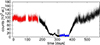 |
Fig. 1. Kepler light curve of MV Lyr during the transition from high to low state and vice versa. The red points represent the high-state interval we selected for the analysis, and the blue points are the selected low state. The shaded area represents the deep low state containing QPOs (see text for details). |
Examples of light curves for individual objects are shown in Fig. 2. All light curves appear to have similar characteristics at first glance, except for MV Lyr in the high state, where well-resolved flares with a timescale up to about 1 ks are present.
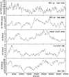 |
Fig. 2. Examples of 0.2−10.0 keV light curves for every analysed object (IRAS 13224−3809 ObsID 0780561601, 1H 0707−795 ObsID 0511580101, and Mrk 766 ObsID 0304030501). All light curves are shown from the beginning of the observation, except for MV Lyr, which is in a low state. The latter starts from day 350 (see Fig. 1). |
3. AFP analysis
The PDS analysis is a very frequently used but generalised technique. The inconvenience is that various structures of a time series with the same or a similar characteristic frequency can blend together and form a single PDS feature. Moreover, if the studied time series is reversed in time, the PDS is unchanged. The same is valid for ACF. This makes the exact timing location of an event difficult, that is, when a side lobe is localised in a rising branch of a flare, the lobe is detected by the ACF, but the location information is lost. On the other hand, the AFP method extracts and conserves not only the Fourier amplitude information of flare events from time-series data, just like PDS and the ACF, but also the relative phase information in between different frequencies related with the flares. Therefore, we applied the AFP method, which yields a result that may be asymmetric and allows us to localise the relative positions of different substructures in time.
The AFP method also has specific disadvantages. When events are superposed by aligning the peaks, especially for low statistical data, count fluctuations smear the fine structure of the profile. Furthermore, higher- and (much) lower-frequency components that are unrelated with the selected peak events are completely ignored (e.g. high-frequency components at > 1 Hz in Cygnus X-1; see Negoro et al. 2001). Furthermore, if the averaged flares have various types of profiles, which occurs in the case of non-stationarity, the current AFP does not provide a true average profile, and the average profile must depend on the criteria that are used to select the flares. The stationarity is discussed in more detail in Sect. 4.1. Finally, when the time bins of the light curve are too short, a false central spike can be created. We investigate this strong artefact in the next section.
3.1. Method
The goal of the AFP method is a direct visualisation of individual PDS components in the flare shape, like in the case of Cyg X-1 (Negoro et al. 2001). The whole idea is supported by simulations of radiation that is generated by an inhomogeneity propagating through advection-dominated flow5 (Manmoto et al. 1996). This inhomogeneity does not dissipate and generates a typical flare profile. Many subsequent inhomogeneities generate many flares that can overlap and are affected by noise. A single flare is not enough for an analysis of the profile, because all faint features are typically hidden in the noise. The summation and averaging of individual flares smooths these contaminations out, and only the original flare remains6.
The method has three steps. The first step is the identification of flares. A light-curve data point is identified as a peak when Npts points to the left and Npts points to the right have lower fluxes than the tested point.
In the second step, the flare extension to be averaged must be defined, in this case, as Nptsext points to the left and right from the peak. Dobrotka et al. (2019) used Nptsext = Npts/2 to avoid superimposing a declining branch of one flare onto a rising branch of the adjacent flare, and vice versa.
The number of XMM-Newton data is much lower than that of the Kepler light-curve data. Therefore, the parameters Npts and Nptsext must be set up with caution. The condition Nptsext = Npts/2 shortens the time extension of the studied flare. This must be compensated by higher values of Npts. However, larger Npts decreases the number of flares per AFP, which increases the noise. Dobrotka et al. (2019) showed that the condition Nptsext = Npts is still acceptable, and any method artefacts occur for Nptsext > Npts. Therefore, for this work, we used Nptsext = Npts. This empirical test also explains why overlapping flares do not contaminate the shape of the AFP. Even when individual selected flares are certainly contaminated by other overlapping flares (see Fig. 3 in Dobrotka et al. 2019), they are redistributed randomly, and the summation of many flares smooths out any randomly redistributed events. Only regularly repeating feature will be seen in the AFP.
In the last step after the flare selection, the flare data points are averaged with the maxima aligned, and the resulting averaged flux minimum value is subtracted from all averaged points. All flares with rare individual null points or missing data (at the edge of the light curve or gaps) were excluded from the averaging process.
The method is described in more detail with several tests, such as the role of the N parameter on the results, or the sampling of Kepler data with an instrumental interruption in Dobrotka et al. (2019). The authors also performed several reality tests, such as a comparison of the AFP with ACF, and found the same features in both methods.
For the XMM-Newton EPIC/pn data of the selected AGNs, we used 100 s bin as an empirical compromise between S/N ratio and resolution. As the parameter Npts, we used 20 and 40, which yielded a time extension of 2000 and 4000 s on either side from the centre of the averaged flare.
For the Kepler data of MV Lyr, we used Npts = 34 and 68 to obtain a similar time extension as for the AGNs. With the Kepler cadence of 58.8 s, the corresponding time extensions are 1999.2 and 3998.4 s. As discussed in Dobrotka et al. (2019), the long-term trend and barycentric correction of Kepler data do not affect the result.
Finally, it is important to exclude one selection effect in the resulting profiles. Since the method first searches for a maximum, this maximum point of a flare can be a scattered point due to count fluctuations towards a higher count rate. This selection effect results in a deviating central point. In Fig. 3 we show simulations of flares using Eq. (1). We used different time bins to show the role of the Poisson noise. Apparently, the method detects the most strongly deviating point and not always the true flare maximum. This detection of the most strongly deviating point results in an accumulation of this systematic bias, and a central false spike appears. The larger the time bin, the smaller the spike bias. Since the method detects the most strongly deviating point because of the Poisson noise, this bias is inherently present in any observed light curve. Moreover, since the method does not detect the real flare maximum, the detected maxima are scattered around the real value. It is easy to demonstrate by simulations that the larger the time bin, the lower this scatter. The simulations in Fig. 3 show that a 100 s time bin yields results where the central spike bias is negligible. This is only valid for the performed simulations with specific parameters, however. In reality, it depends on the flare amplitude and mean count rate, that is, on parameters that affect the Poisson noise level. Since this artificial count increase only affects a single central point, any real substructure such as a real central spike must be represented by more than one single point. The single central point consists of the real flux level of the flare maximum and the Poisson-noise artefact. With the recent method, it is impossible to separate the real flux level and the false contribution.
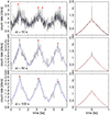 |
Fig. 3. Simulated light curves with AFPs. Left panels: Light curves with synthetic flares using Eq. (1) and Fc = 2 cts/s, Fc = 0.5 cts/s, Tr = Td = 1000 s with Poisson noise. Different time bins Δt are shown. The detected flare maxima are shown as red points. Blue shows the original light curve without noise. Right panels: AFPs calculated from synthetic light curves with 200 flares. The red line depicts the reference light curve without noise. |
Moreover, in the case of the shortest time bins, even two maxima can be detected for one single flare when the count rate is the same (top panel of Fig. 3). Another artefact is some flattening of the averaged flare close to the central false spike. This effect is negligible in simulations with a time bin of 100 s. Apparently, this flattening is related to the central spike bias, and it is probably generated by non-aligned flares before averaging. A time bin that is large enough reduces the central spike bias and also the central flattening.
Therefore, we used a 100 s bin for all X-ray light curves as a compromise between scatter and time resolution. In order to exclude any potential central spike bias when comparing individual AFPs, we excluded the central point from all profiles since the scatter and flare amplitudes are different from one source to the next. Subsequently, we normalised the averaged flare flux by its remaining maximum value. All other analyses, such as the comparison of individual amplitudes in a single source or the profile fitting, were performed in standard count rates without any modification. The central point alone was not taken into account during the fitting procedure.
On the other hand, the exclusion of the central point can have a negative impact. It smears possible short-term variations associated with the flare. A solution would be to identify flares in a different way. For example, finding the highest point can be just a step to identify a possible flare maximum, and the true flare can be selected by fitting a typical profile (described in the next section). However, as mentioned and demonstrated in Fig. 3 of Dobrotka et al. (2019), the flares does not have a typical profile because of contamination by adjacent flares. The shapes are very different, with sharper and wider peaks, clearly decreasing or increasing branches, or variable branches with strong humps or plateau with a constant count rate, and so on. Our situation is very different from the case of fast variability in the BH in the hard state (Negoro et al. 1994; Focke et al. 2005) and blazars (Sasada et al. 2017), or stellar flares (Tovar Mendoza et al. 2022) and gamma-ray bursts (Sakamoto et al. 2007), where the flares are relatively isolated. They are likely suitable for fitting with a typical profile. The difference in flare behaviour is not only a technical challenge or difficulty. It says something about the origin of the variability and physical conditions in the accretion flow.
The central region importance is clearly seen in the stellar flare shape, where it has been shown that the flare profile does not have break points between the rise and decay, but a continuous model where the peaks roll over is needed instead (Kowalski et al. 2016; Jackman et al. 2018, 2019; Howard & MacGregor 2022). Nevertheless, in this work, we only focus on wider patterns such as side lobes or the central spike, rather than the peak itself. Therefore, we accept the exclusion of the central point because it does not affect the studied flare features.
3.2. Results
The resultant AFPs are depicted in Fig. 4, and the numbers of the averaged flares are summarised in Table 1. Clearly, all the AGN profiles are very similar, except for those of IRAS 13224–3809, which show a noticeable side lobe between −3200 and −1000 seconds. The most important result is the indistinguishable resemblance of the MV Lyr case in the low state, while the profile is totally different in the high state. Apparently, the central spike in the CV and the side lobe(s) make the case different7.
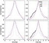 |
Fig. 4. Averaged flare profiles for two different time extensions (from −2 to 2 ks in the left panels, from −4 to 4 ks in the right panels). The three AGNs are compared to CV MV Lyr. The latter is shown in two different states: in a low (upper panels) and high (lower panels) state. The averaged number of the flares is summarised in Table 1. The thick black line shows the side lobe between −3.2 and −1 ks of IRAS 13224–3809, as discussed in the text. |
Number of averaged flares for individual time extensions.
Multiplying the MV Lyr profiles in the high state by a factor of a few lifts them up. As a result, the central spike is out of the figure, and we can only compare the wider base of the CV with the bases of the AGNs. The left panel of Fig. 5 shows that the profile more or less agrees with the AGN profiles. However, the right panel is more interesting because it shows a larger time extension. Not only the overall profile matches the AGN cases, but the left side-lobe also matches a similar structure seen in IRAS 13224–3809. Since the MV Lyr profile is calculated from 2631 flares, this structure is unambiguous.
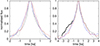 |
Fig. 5. Same as bottom panels of Fig. 4, with the MV Lyr case multiplied by 3 (left panel) and 2 (right panel). |
Alston et al. (2019) and Caballero-García et al. (2020) divided the IRAS 13224–3809 light curve into low, medium, and high states. We did the same, and for simplicity, we divided the light curve into high, low-medium, and low-flux data. Three observations have a remarkably higher mean flux (higher than 4 cts/s) and variability amplitude (square root of the variance). These are classified as high-flux data. The observations with a mean flux lower than 2.5 cts/s represent low-flux data, and the rest are low-medium data. The left panel of Fig. 6 compares the averaged flares from all three light-curve subsamples. We focus on the largest time extension from −4 to 4 ks, where IRAS 13224–3809 shows a side lobe in the rising part of the flare. Clearly, this side lobe is dominant in the high-flux flare. The lower the flux, the closer the averaged profile to the other three objects. In general, the high-flux case tends to be wider in the time interval from −3 to 2 ks, while the low-flux case matches the other objects well.
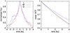 |
Fig. 6. Averaged flare profiles of IRAS 13224–3809 with the corresponding ACFs. Left panel: Same as the upper right panel of Fig. 4, but the IRAS 13224–3809 flares are calculated from low- (red line), low-medium (black line), and high- (blue line) flux subsamples of the IRAS 13224–3809 light curve. Right panel: Mean ACFs of the same light-curve subsamples of IRAS 13224–3809. |
In order to study the energetics of the flares, we divided the light curve into soft (below 1 keV) and hard (above 1 keV) bands. Most photons are below 1 keV. Therefore, if we would like to have the same number of photons in both bands, we would need to use an energy lower than 0.6 keV as the threshold energy. This is too low for a meaningful energetic study8. The comparison of IRAS 13224–3809 AFPs in the different energy bands are plotted in Fig. 7. We again focus on the largest time extension, where IRAS 13224–3809 shows a side lobe in the rising part of the flare. When the whole light curve is used, the flare width in the hard band is narrower than in the soft band, and the side lobe on the rising branch is not seen (left panel of Fig. 7). When we only compare high-flux flares from Fig. 6, the corresponding hard band is slightly wider, but there is no significant difference in the side lobe (right panel of Fig. 7). This means that the side lobe is present in both bands during the high-flux period, but is absent in the lower-flux periods.
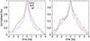 |
Fig. 7. Comparison of IRAS 13224–3809 AFPs in the soft and hard bands together with that from the whole energetic interval. The left panel represents the same as Fig. 4, and the right panel only compares high-flux intervals, like in Fig. 6. |
The meaning of the AFP is the possibility to see the timescales directly. The individual profiles are best described by the following exponential function (Sasada et al. 2017; Dobrotka et al. 2019):
 (1)
(1)
where t is the time, and Tr and Td are the time constants of a rising and declining branch, respectively. These time constants correspond to knees in the PDS with frequencies of 1/(2πTr) and 1/(2πTd). Fc and F0 represent the constant level and the amplitude of the flares, respectively. We excluded the central point at 0 s from the fitting for the reasons described above.
The fits are shown in Fig. 8, and the parameters are summarised in Table 2. The first fits of the flares with a time extent of 2 × 2000 s (Npts = 20) describe all the profiles well. On the other hand, there is a problematic structure in the time extent of 2 × 4000 s (Npts = 40). Strong deviations from the model function appear in the case of IRAS 13224–3809. The rising branch does not have a smooth development, and it has the side lobe mentioned above. We selected a region in which this lobe is clearly seen, and we excluded this time interval from the fitting procedure (shaded area in Fig. 8 and blue line). Apparently, the two fits yield different timescales in the case of IRAS 13224–3809. Therefore, it is better to treat this case in more detail. Figure 9 shows the high- and low-flux version of the flares with fits. In the former, we only fitted the rising part of the flare in the selected time interval. The fit describes the beginning of the side lobe well. Finally, the low-flux AFP is well fitted without any significant deviation.
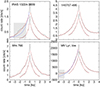 |
Fig. 8. Fits to the averaged profiles from Fig. 4 using Eq. (1). The red lines represent the fits to the whole time extension, and the blue lines are fits after some time-interval exclusion (shaded areas). |
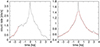 |
Fig. 9. Same as Fig. 8, but only for high- (left panel) and low- (right panel) flux flares of IRAS 13224–3809. |
Tr and Td parameters and corresponding PDS characteristic frequencies fr and fd for individual objects. text is the time extension of the averaged flare.
A problematic fitting behaviour is also seen in the rising branch of the MV Lyr AFP in the low state. The profile rises from approximately −3000 s towards lower time values. We selected this time region and excluded it from the fitting procedure (shaded area in Fig. 8 and blue line).
Apparently, none of the characteristic frequencies reaches log(f/Hz) = −3 seen in the high state of MV Lyr or in IRAS 13224−3809 (Alston et al. 2019). To obtain this frequency from the exponential rise or decay profile, the Tr or Td parameter should be about 160 s. The timescale of 160 s corresponds to only two time bins, and Npts = 6 or less is required for averaging the IRAS 13224–3809 flares and fitting up to or from 0 s (central point included). Therefore, the resolution of the very central part of the spike is too low for a detection of the log(f/Hz) = −3 frequency (if present).
The fitted Tr and Td parameters vary from one object to the next, and the time constants depend on the time extension to be investigated. All the corresponding frequencies log(f/Hz) are, however, in the range of −3.5 to −4.1, including MV Lyr. We also note that the average time constants of Tr and Td in 1H 0707−495 and MV Lyr are only different by less than 20% in the two time-extension fits, which implies that these values are characteristic time constants of these objects. Indeed, Tr + Td (∼2000 s) of 1H 0707−495 is about half of the 3800 s QPO periodicity observed in the XMM-Newton, observations (Pan et al. 2016; Zhang et al. 2018).
Finally, it is worthwhile to compare the AFPs from individual observations. To increase the number of averaged flares, we used a time extension of only 2000 s (from −1000 to 1000 s, Npts = 10). Individual profiles are shown in Fig. 10.
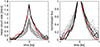 |
Fig. 10. Averaged flare profiles from individual observations. The thick lines represent the ObsIDs 0780561601 (red), 0792180401 (black), and 0792180601 (black). The left panel represents the true amplitudes. The right panel shows the same comparison as in Fig. 4, where the central point is excluded and the resulting maxima are set to 1. |
All profiles have very similar amplitudes, except for three cases that are considerably higher (shown as thick lines). All three observations are those already mentioned, with the highest mean fluxes and variability amplitudes. The three averaged profiles are very similar. Some minor deviations in ObsID 0780561601 shown as the red line are possible in the wings below −500 and above 200 s. The other two profiles (ObsIDs 0792180401 and 0792180601) represented by black lines are almost identical. However, due to the very low number of averaged flares (48 red, 45 and 49 black), we cannot say whether these faint details are real. Moreover, as shown in the lower panel of Fig. 10, all profiles are comparable, just the scatter of the low-amplitude cases is too large due to the low number of counts. The conclusion is that at least the three dominant profiles show similar slopes or curvatures, without any obvious substructure such as a side lobe in the time interval of −1000 to 1000 s.
3.3. Comparison with the ACF
Dobrotka et al. (2019) compared the AFP with the ACF and found the same features in both methods. We performed the same confidence test.
As the ACF requires continuous uninterrupted light curves, we calculated ACFs of individual XMM-Newton observations and averaged them. MV Lyr data were divided into subsamples separated by larger gaps. This resulted in three and six subsamples for the low and high state, respectively. Sporadic zero points were removed and replaced by median values using a Hampel filter9.
The differences in ACFs are clear in Fig. 11. The mean ACFs of AGNs and CV in the low state are smooth and monotonic. In contrast, the CV in the high state shows a structured ACF, with a steep decline followed by a small hump, which represent the central spike and the side lobes, respectively. After the small hump, the ACF continues monotonically as in the AGN cases.
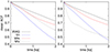 |
Fig. 11. Comparison of mean ACFs. The left panel compares AGN ACFs with the ACF of CV MV Lyr in a low state, and the right panel shows MV Lyr in a high state. |
The same confidence test can be applied to the side lobe in the rising part of the flare, depicted in the right panel of Fig. 6. The mean ACFs calculated from the same light-curve subsamples are depicted in the left panel of Fig. 6. The difference between low- and low-medium flux AFPs is small, but the difference is already seen. The same is valid for the corresponding ACFs. The largest difference is seen in high-flux profile, which agrees with the highest difference in ACFs. The studied side lobe starts to deviate from other profiles at approximately −1 ks. The ACFs also deviate from approximately 1 ks. Apparently, the ACFs support the existence and flux dependence of the side lobe detected in the AFP of IRAS 13224–3809.
4. Discussion
We performed an AFP analysis of three selected AGNs observed with XMM-Newton. We compared the results with the AFP of the CV MV Lyr observed with Kepler spacecraft.
One of the selected AGNs is IRAS 13224–3809. This AGN has the longest observation list in the XMM-Newton archive, which makes it suitable for a more detailed analysis. We searched for characteristic frequencies and for any relation between the AFP and the standard PDS.
4.1. Stationarity
Our AFP method selects flares and averages them in order to obtain a mean typical profile from the whole light curve. Therefore, the method is ideal for stationary processes in which the shape of the flare does not change in time. Alston et al. (2019) reported that the XMM-Newton data of IRAS 13224–3809 show evidence for non-stationarity. The authors compared PDSs calculated from several epochs. They concluded that the PDSs are well described by two peaked components, and the non-stationarity is seen as clear changes in the PDS normalisation as well as smaller changes in the PDS shape, that is, a shift in the peak frequency of the low-frequency component close to log(f/Hz) = −4.3. When only the normalisation (power) of the PDS features changes, any break or QPO frequency should be unchanged, and this is what we searched for in the AFP.
However, the smaller shift in the low-frequency component can affect the AFP. The changes are only small, however, and Alston et al. (2019) concluded that the PDSs have similar shapes from one epoch to the next, and the variability components cannot vary dramatically. Therefore, we investigated individual observations of IRAS 13224–3809 and obtained similar AFPs showing some scatter because we do not have enough counts, except in three cases (Fig. 10). These three cases from different epochs show very comparable AFPs. This implies that either all three observations with a higher flux have comparable characteristics, or that any non-stationarity within different epochs has no significant impact on the AFP. Any change in the PDS components is hidden in the noise of the AFPs.
4.2. Comparison of the AFP substructure with the PDS in IRAS 13224–3809
The remarkable observations of IRAS 13224–3809 by XMM-Newton allowed us to study the AFP in more detail, and we also studied its evolution in time. First, we point out the similarities between our AFP analysis and the PDS studied by Alston et al. (2019). Our AFP fitting revealed potential characteristic frequencies at log(f/Hz) = −3.47, −3.70, −3.97, or −4.06 (Table 2). These values correspond to the bend frequency interval from 8.7 × 10⁻⁵ to 3.4 × 10⁻⁴ Hz in the 1.2−3 keV and 3−10 keV bands, shown as blue and grey histograms in Fig. 10 (panel a) of Alston et al. (2019) using the bend1 + bend2 + lor1 model. The same energy band of 1.3−3 keV also shows a bend frequency at approximately 1 − 2 × 10⁻³ Hz, shown as the blue histogram in Fig. 10 (panel b) of Alston et al. (2019). This bend frequency suggests a time constant of ∼100 s in Eq. (1). For such high frequencies, we apparently lack the resolution. They imply that our AFP involves the low-frequency properties of the observed PSD.
The AFP consists of two (sub)structures: A main flare10 described by one or two exponential functions in the rise and decay, and a large side lobe during a higher overall flux (Fig. 12). We also note that the averaged flare of Cyg X-1 has a similar side-lobe structure in the rising phase (Negoro et al. 2001). We discuss individual substructures and their physical meaning below.
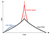 |
Fig. 12. AFP substructures. A central spike is seen only in CV MV Lyr during the high state. If a false spike due to Poisson noise appears, it is on top of the real central spike and confuses the maximum flux (dotted red line). When no real spike is present, the false spike can appear on top of the main flare, as in Fig. 3 (dotted black line). |
4.3. Optical versus X-ray AFPs
It is important to explain first why we compare optical radiation in CVs with X-rays in AGNs. Based on the accretion fluctuation propagation scenario, every inhomogeneity that is generated in the outer disc regions propagates inwards. All subsequent mass-accretion fluctuations during the accretion flow are coupled, and this modulates the X-ray radiation that is liberated in the inner disc. Every fluctuation entering the corona from the inner disc must therefore modulate the optical radiation from the inner disc and the X-rays liberated in the corona. The similarity of the profiles implies that the physical sources of optical light and X-rays are close or correlated.
Another possible explanation is based on the reprocessing of X-rays into the optical, as was proposed in the MV Lyr case (Scaringi 2014). In this case, the geometrically thick corona surrounding the geometrically thin disc radiates in X-rays. These X-rays are reprocessed by the underlying thin disc. In the case of CVs and AGN with truncated discs, the central evaporated accretion flow (corona) can be the source of X-rays that irradiate the inner disc. The latter then reprocesses the X-rays into optical radiation. Similar flare profiles are then expected.
However, the reprocessing situation is not the same in AGNs and CVs. Alston et al. (2019) concluded that the UV PDS in IRAS 13224–3809 behaves very differently compared to X-rays. This suggests a different physical origin of the variability and does not support the reprocessing scenario. Nevertheless, the X-ray variability is generated in the X-ray corona. In contrast, the PDS in the optical (Scaringi et al. 2012a), UV, and X-rays (Dobrotka et al. 2017) in MV Lyr has the same characteristics, which suggests reprocessing. Therefore, the optical variability in MV Lyr is an image of the X-ray variability that is generated by the corona. This suggests that our motivation to compare the two bands in AGNs and in MV Lyr is justified.
4.4. AFPs in AGNs versus CVs
While CVs in the high state have discs that develop up to the WD surface, quiescent discs are truncated. The latter are more similar to AGNs, whose discs are likely also truncated. This implies an explanation for the similarity of the quiescent AFP in MV Lyr to AGNs. We assumed that the very central part of the disc is the source of the optical central spike in the AFP of MV Lyr. CVs in the high state have this inner disc, while quiescent CVs and AGNs do not. As a consequence, the central spike disappears in systems with truncated discs.
The situation is depicted in Fig. 13. It is still unclear what the corona looks like. It is some hot plasma near the BH. Many authors used the lamp-post model, in which the corona is above the BH on the rotation axis (Martocchia & Matt 1996). We investigated the sandwich model, in which the corona is produced by evaporation (Meyer & Meyer-Hofmeister 1994) above or below the geometrically thin disc, and where it forms a geometrically thick disc. In the innermost regions, the geometrically thin disc completely evaporates (is truncated), and an advection-dominated accretion flow forms (see e.g. Różańska & Czerny 2000). This flow may act as a corona and yields a complex accretion geometry (see e.g. Fig. 2 in Liu & Taam 2009 or Fig. 9 in Wilkins et al. 2014). The principal idea of the inner disc as a reprocessing region is also valid for the lamp-post geometry, however.
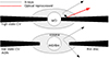 |
Fig. 13. Accretion geometry with a WD, BH, and geometrically thin and thick (corona) discs. The arrows show the native X-ray and reprocessed radiations. |
According to this scenario, some substructures of the flare profile are generated by the truncated disc (main flare), while another (central spike) is added during the high state of MV Lyr. Figure 5 shows this situation, that is, when we ignore the central spike of the MV Lyr AFP in the high state and rescale it, we can find a solution in which the CV profile is similar to those of the AGNs.
As already mentioned, the X-ray PDS of IRAS 13224–3809 shows significant PDS patterns at log(f/Hz) ≃ −3 that are represented by a narrow Lorentzian plus a broad component (Alston et al. 2019). MV Lyr shows a rather broad component at log(f/Hz) ≃ −3 in the corresponding X-ray (Dobrotka et al. 2017) and optical PDS (Scaringi et al. 2012a). Therefore, the broad component in IRAS 13224–3809 is of interest to us (Fig. 9 in Alston et al. 2019). In the case of MV Lyr, the PDS bump structure at log(f/Hz) ≃ −3 results from sharp peaks (central spike) of the flares with time constants of about 200 s and side lobes at about −640 s and 740 s from the flare peak (Dobrotka et al. 2019). Unfortunately, in the case of IRAS 13224–3809 flare, we did not find direct evidence for this frequency because the resolution was not high enough.
It is very attractive to connect this PDS feature at log(f/Hz) ≃ −3 to the same frequency component as detected in MV Lyr during the high state, which is absent in the low state. This fits the corona inner disc interpretation in the AGN as follows: If the corona is the source of such variability, the PDS pattern should also be seen in X-rays in the AGN with a truncated disc because the corona is present. Only the optical and UV counterpart should be absent because the inner disc as the reprocessing region is missing (see the model in Fig. 13). This is what we observe in IRAS 13224–3809, that is, the log(f/Hz) ≃ −3 signal is seen in X-rays, but is absent in the UV. In MV Lyr in the high state, the optical PDS matches the X-ray one, but we lack a detailed X-ray observation during the low state. If the corona interpretation is correct, the X-ray PDS of MV Lyr in the low state may show the log(f/Hz) ≃ −3 structure, although the optical PDS did not show this structure (Dobrotka et al. 2020).
4.5. Side lobes in IRAS 13224–3809
In addition to the main flare, we also detected a large side lobe during the higher overall flux (Fig. 12). It appears before the maximum, which suggests that the physical mechanism that causes it must be present before the main source of the flares.
The amplitude of this substructure increases with increasing overall flux. The increased flux is probably due to an increased mass-accretion rate. This process can result from a modification in the accretion-flow geometry. We assumed that the corona has the shape of a sandwich (Fig. 13). The physical explanation of a geometrically thick disc like this is based on the evaporation of matter due to inefficient cooling via free-free transitions (Meyer & Meyer-Hofmeister 1994). The more radially distant regions of the thin disc evaporate partially, while the innermost parts evaporate completely. During the higher-flux period, this corona can expand radially outwards because if more matter flows through the geometrically thin disc, more energy is generated in the outer disc regions. Therefore, more radially distant regions can evaporate. A similar interpretation was offered by Kara et al. (2013) based on soft time lags in IRAS 13224–3809 and by Wilkins et al. (2014) by modelling the relativistically broadened iron Kα fluorescence line in 1H 0707–495. The authors assumed that the X-ray source is more compact during low-flux intervals. However, there is no reason to expect any substructure in the flare profile. A radially expanded corona like this would generate mass-accretion fluctuations on a longer timescale. Rather a wider flare would be generated, which we did not observe.
A combination of the corona as a sandwich and some central regions similar to the lamp-post substructure is a possible speculation. Here, the lamp post is not always necessary, but some powerful energy source that reflects the deep gravitational potential well near the central part of the disc is necessary (see e.g. Fig. 4 in Zdziarski et al. 2021). Therefore, we refer to it as the very central part of the corona. In this scenario, the radially extended sandwich corona can be a weak source of X-rays during the low-flux periods. Any side lobe generated by this corona would be too weak, and only the very central source would generate a central structure of the flare that is strong enough to be detected. If the flux increases, the higher mass-accretion rate results in a higher particle density n of the corona. This hot corona radiates via free-free processes, in which the emissivity is proportional to n2. Any mass accretion fluctuation entering this denser corona first becomes observable as increased radiation from the sandwich corona. Subsequently, the fluctuation enters the very central region, where it radiates more prominently.
Alternatively, the sandwich corona is too compact and localised only in the very central regions close to the BH during the low-flux state. As a consequence, the side lobe blends with the main flare, that is, the two substructures cannot be distinguished. During the high-luminosity state, the sandwich-shaped corona is radially more extended, allowing the side lobe to be distinguished from the main flare. This scenario is practically the same as the previous one. The radially more extended corona is just the case where the emissivity due to larger n is sufficient up to larger radii.
Even though the proposed scenario is too speculative, the side lobe in the AFP suggests that an additional source of X-rays appears during the high-flux period. This source should appear earlier in the accretion flow because it precedes the main flare. The described scenario is an independent confirmation of the similar process discovered by Wilkins et al. (2014). The authors studied X-ray observations of Mrk 335 and described the evolution of the corona geometry during flux variability. On long timescales, they found that during the high-flux epochs, the corona expanded, and it subsequently contracted to a more compact form in the intermediate- and low-flux epochs.
However, we found that the rise profiles in MV Lyr and the AGNs are very similar. If the main flare is associated with the very central substructure, such as the lamp-post part of the corona, the similarity can imply a similar corona geometry in CVs as well. It is hard to conclude whether CVs also have this lamp-post substructure of the corona, but CVs certainly have boundary layers. Based on the similarity of the AFPs, some very central corona substructure could be the equivalent of the boundary layer in CVs. However, the energetics can be challenging because in BH discs, approximately half of the gravitational energy is released in the disc (see e.g. Pringle 1981), and the rest of energy is lost (disappears into a BH). On the other hand, in CVs and neutron star cases, the rest of energy is expected to be released on the surface of the star or in the boundary layer. Therefore, the energy release in the case of AGN should be less effective, which is hard to compare with MV Lyr AFP since our AGN and CV data are not in the same band. In both AGNs and CVs, the mass-accretion fluctuation in any case first propagates in the sandwiched corona, modulates the local radiation, and subsequently enters the very central substructure in AGNs, or the boundary layer in CVs, where the main flare is generated.
So far, we described the inner accretion flow as a combination of a cold geometrically thin disc and a hot geometrically thick corona. However, AGNs show a soft excess, suggesting an optically thick warm medium. This medium can be a warm corona located in the inner parts of the accretion disc (see e.g. Mehdipour et al. 2011; Jin et al. 2012; Różańska et al. 2015; Petrucci et al. 2018) and localised just outside the hot optically thin corona (Kubota & Done 2018). If this warm corona is the speculated structure that is located before the source of the main flare, it should mainly be seen in soft X-rays. This is shown in Fig. 7. Apparently, the side lobe is only seen in soft X-rays. When we take only the high-flux interval, however, this dominance in soft X-rays disappears, which is puzzling and complicates the warm-corona interpretation.
Finally, the comparison of soft and hard bands in Fig. 7 recalls the study of Cyg X-1 using ACF, which is a symmetric equivalent of the AFP (Dobrotka et al. 2019). This ACF function study of Cyg X-1 was performed by Maccarone et al. (2000). The authors found that the ACF is narrower in the hard band and proposed drifting blobs in a hot corona as a source of the studied fast variability. These drifting blobs can be an equivalent of the propagating mass-accretion fluctuations.
Alternatively, different scenarios can be considered. The side lobe may be a precursor of the flare, for instance, the magnetic reconnection in an outer part of the accretion disc. Maccarone et al. (2000) proposed magnetic flaring as another option to explain the observed narrowing of the ACF in harder bands.
4.6. Typical flare profile
As discussed in Dobrotka et al. (2019) for MV Lyr, an aperiodic mass accretion is most likely to produce the rise part of the flare. The basic idea is based on an accretion fluctuation propagation model, which is generally accepted as the main source of the flickering in AGNs and CVs. In the model, when the accretion fluctuation reaches the innermost part of the accretion disc, the maximum gravitational energy is released, resulting in an observed relatively sharp peak. Since all accretion fluctuations release energy by the same process and at the same distance from the centre, all corresponding flares have the same profile and timescale. As a consequence, the width of the flare representing the typical timescale depends on the inner disc radius, as shown in Fig. 13. The greater the depth in the potential well at which the flare is generated, the narrower the flare. This is clearly seen in MV Lyr, where we know the difference in the disc between the high and low state well. In the high state, the disc develops (almost) down to the WD surface, the viscous timescale is short, and a very narrow central spike is seen. In the low state, in contrast, the disc is truncated and the flare is generated farther away and has a considerably wider shape because the viscous timescale is longer. The only variable quantity is the amount of matter in the accretion fluctuation. This affects the quantity of the released energy, which induces the amplitude.
Finally, the decay of the flare may be produced by an acoustic wave, as shown by Manmoto et al. (1996). Moreover, there is the impression that the profiles are very similar on either side of the flare. It is beyond the scope of this work to investigate this, but following the Tr and Td parameters in Table 2, the profiles on either side can have different timescales. The case is variable from one object to to the next and depends on the time extension that is used for the fitting. Therefore, the similarity of the two sides of the flare is not justified, and it can be just a coincidence or can have a real physical explanation.
5. Summary and conclusions
We analysed XMM-Newton observations of three selected AGNs. We studied the AFPs. We did the same with Kepler data of the CV MV Lyr. It appears that all flares have a similar shape when the CV is in quiescence. This conclusion was supported by the direct fitting of the flares, which yielded comparable timescales in all four objects. We explained this similarity by the existence of a truncated inner disc. This truncation is absent in the high state of the CV, where the disc develops (almost) up to the WD surface. This supports the reprocessing scenario, in which the X-rays are generated by the corona. These X-rays are reprocessed into optical radiation by the underlying geometrically thin disc in the so-called sandwich model. When the disc is truncated, the central disc as the reprocessing region is missing, and no X-ray variability is seen in the optical.
We performed a more detailed analysis of AGN IRAS 13224–3809 because it has the most extensive XMM-Newton light curve. Alston et al. (2019) found low- and high-frequency PDS patterns below or close to log(f/Hz) = −4 and above or close to log(f/Hz) = −3, respectively. Our direct fitting of the AFP only identified the low-frequency component close to log(f/Hz) = −4.
The IRAS 13224–3809 AFP shows a larger side lobe on the rising branch. We divided the light curve into low-, low-medium, and high-flux subsamples. The side lobe does not have the same amplitude in the corresponding AFPs. It is strongest in high-flux data, but practically absent in the low-flux data. We interpreted this as a double-structured corona with a sandwich part and some very central substructure. Any mass-accretion fluctuation enters the sandwich corona and generates the side lobe. Subsequently, it propagates through it and reaches the very central region, where the main part of the flare is radiated. The sandwich corona is weak during the low-flux periods, and any radiated patterns only become visible during high-flux states.
Negoro et al. (1994) used the word “shot”.
ObsIDs: 0110890101, 0673580101, 0673580201, 0673580301, 0673580401, 0780560101, 0780561301, 0780561401, 0780561501, 0780561601, 0780561701, 0792180101, 0792180201, 0792180301, 0792180401, 0792180501, 0792180601.
ObsIDs: 0673580101, 0673580201, 0673580301, 0673580401, 0780560101, 0780561301, 0780561401, 0780561501, 0780561601, 0780561701, 0792180101, 0792180201, 0792180301, 0792180401, 0792180501, 0792180601.
ObsIDs: 0096020101, 0109141301, 0304030101, 0304030301, 0304030401, 0304030501, 0304030601, 0304030701, 0763790401.
Manmoto et al. (1996) did not consider the origin or seed of the inhomogeneity. They only showed what happens when fluctuation is present in the advection flow. The inhomogeneity can be an accretion fluctuation or a turbulence.
It is important not to confuse the method with the shot-noise process, in which individual flares are summed to obtain a simulated light curve. This process is additive, which is not consistent with observations. The summation and averaging of many flares in our method is done for the smoothing, not for the construction of a light curve.
We note that the central spike of MV Lyr consists of more than one single central point, and therefore, it is a real structure.
We tried two such bands, and we did not see significant difference between soft and hard AFPs.
Python hampel library https://github.com/MichaelisTrofficus/hampel_filter
The main flare in AGNs is equivalent to the wider base around the central spike in MV Lyr during the high state (Fig. 5).
Acknowledgments
AD was supported by the Slovak grant VEGA 1/0576/24. HN was partially supported by Grants-in-Aid for Scientific Research (21K03620) from the Ministry of Education, Culture, Sports, Science and Technology (MEXT) of Japan. We thanks the anonymous referee for very helpful comments concerning the averaged flare profile method.
References
- Alston, W. N., Fabian, A. C., Buisson, D. J. K., et al. 2019, MNRAS, 482, 2088 [NASA ADS] [CrossRef] [Google Scholar]
- Arévalo, P., & Uttley, P. 2006, MNRAS, 367, 801 [Google Scholar]
- Benlloch, S., Wilms, J., Edelson, R., Yaqoob, T., & Staubert, R. 2001, ApJ, 562, L121 [NASA ADS] [CrossRef] [Google Scholar]
- Bhargava, Y., Hazra, N., Rao, A. R., et al. 2022, MNRAS, 512, 6067 [NASA ADS] [CrossRef] [Google Scholar]
- Boller, T., Keil, R., Trümper, J., et al. 2001, A&A, 365, L146 [NASA ADS] [CrossRef] [EDP Sciences] [Google Scholar]
- Borisov, G. V. 1992, A&A, 261, 154 [NASA ADS] [Google Scholar]
- Buisson, D. J. K., Lohfink, A. M., Alston, W. N., & Fabian, A. C. 2017, MNRAS, 464, 3194 [Google Scholar]
- Buisson, D. J. K., Lohfink, A. M., Alston, W. N., et al. 2018, MNRAS, 475, 2306 [NASA ADS] [CrossRef] [Google Scholar]
- Caballero-García, M. D., Papadakis, I. E., Dovčiak, M., et al. 2020, MNRAS, 498, 3184 [CrossRef] [Google Scholar]
- Chiang, C.-Y., Walton, D. J., Fabian, A. C., Wilkins, D. R., & Gallo, L. C. 2015, MNRAS, 446, 759 [NASA ADS] [CrossRef] [Google Scholar]
- Dobrotka, A., Ness, J.-U., & Bajčičáková, I. 2016, MNRAS, 460, 458 [Google Scholar]
- Dobrotka, A., Ness, J.-U., Mineshige, S., & Nucita, A. A. 2017, MNRAS, 468, 1183 [Google Scholar]
- Dobrotka, A., Negoro, H., & Mineshige, S. 2019, A&A, 631, A134 [NASA ADS] [CrossRef] [EDP Sciences] [Google Scholar]
- Dobrotka, A., Negoro, H., & Konopka, P. 2020, A&A, 641, A55 [EDP Sciences] [Google Scholar]
- Edelson, R., Vaughan, S., Malkan, M., et al. 2014, ApJ, 795, 2 [NASA ADS] [CrossRef] [Google Scholar]
- Emmanoulopoulos, D., McHardy, I. M., & Papadakis, I. E. 2011, MNRAS, 416, L94 [NASA ADS] [CrossRef] [Google Scholar]
- Fabian, A. C., Miniutti, G., Gallo, L., et al. 2004, MNRAS, 353, 1071 [Google Scholar]
- Fabian, A. C., Zoghbi, A., Ross, R. R., et al. 2009, Nature, 459, 540 [Google Scholar]
- Fabian, A. C., Kara, E., Walton, D. J., et al. 2013, MNRAS, 429, 2917 [NASA ADS] [CrossRef] [Google Scholar]
- Focke, W. B., Wai, L. L., & Swank, J. H. 2005, ApJ, 633, 1085 [NASA ADS] [CrossRef] [Google Scholar]
- Howard, W. S., & MacGregor, M. A. 2022, ApJ, 926, 204 [NASA ADS] [CrossRef] [Google Scholar]
- Jackman, J. A. G., Wheatley, P. J., Pugh, C. E., et al. 2018, MNRAS, 477, 4655 [NASA ADS] [CrossRef] [Google Scholar]
- Jackman, J. A. G., Wheatley, P. J., Pugh, C. E., et al. 2019, MNRAS, 482, 5553 [NASA ADS] [CrossRef] [Google Scholar]
- Jiang, J., Parker, M. L., Fabian, A. C., et al. 2018, MNRAS, 477, 3711 [NASA ADS] [CrossRef] [Google Scholar]
- Jin, C., Ward, M., Done, C., & Gelbord, J. 2012, MNRAS, 420, 1825 [Google Scholar]
- Kara, E., Fabian, A. C., Cackett, E. M., Miniutti, G., & Uttley, P. 2013, MNRAS, 430, 1408 [NASA ADS] [CrossRef] [Google Scholar]
- Kotov, O., Churazov, E., & Gilfanov, M. 2001, MNRAS, 327, 799 [Google Scholar]
- Kowalski, A. F., Mathioudakis, M., Hawley, S. L., et al. 2016, ApJ, 820, 95 [NASA ADS] [CrossRef] [Google Scholar]
- Kraicheva, Z., Stanishev, V., & Genkov, V. 1999, A&AS, 134, 263 [NASA ADS] [CrossRef] [EDP Sciences] [Google Scholar]
- Kubota, A., & Done, C. 2018, MNRAS, 480, 1247 [Google Scholar]
- Lasota, J. 2001, New Astron. Rev., 45, 449 [Google Scholar]
- Liu, B. F., & Taam, R. E. 2009, ApJ, 707, 233 [NASA ADS] [CrossRef] [Google Scholar]
- Lyubarskii, Y. E. 1997, MNRAS, 292, 679 [Google Scholar]
- Maccarone, T. J., Coppi, P. S., & Poutanen, J. 2000, ApJ, 537, L107 [NASA ADS] [CrossRef] [Google Scholar]
- Manmoto, T., Takeuchi, M., Mineshige, S., Matsumoto, R., & Negoro, H. 1996, ApJ, 464, L135 [NASA ADS] [CrossRef] [Google Scholar]
- Markowitz, A., Papadakis, I., Arévalo, P., et al. 2007, ApJ, 656, 116 [CrossRef] [Google Scholar]
- Martocchia, A., & Matt, G. 1996, MNRAS, 282, L53 [NASA ADS] [CrossRef] [Google Scholar]
- McHardy, I. M., Connolly, S. D., Peterson, B. M., et al. 2016, Astron. Nachr., 337, 500 [NASA ADS] [CrossRef] [Google Scholar]
- Mehdipour, M., Branduardi-Raymont, G., Kaastra, J. S., et al. 2011, A&A, 534, A39 [NASA ADS] [CrossRef] [EDP Sciences] [Google Scholar]
- Meyer, F., & Meyer-Hofmeister, E. 1994, A&A, 288, 175 [NASA ADS] [Google Scholar]
- Narayan, R., & Popham, R. 1993, Nature, 362, 820 [NASA ADS] [CrossRef] [Google Scholar]
- Negoro, H., & Mineshige, S. 2002, PASJ, 54, L69 [CrossRef] [Google Scholar]
- Negoro, H., Miyamoto, S., & Kitamoto, S. 1994, ApJ, 423, L127 [NASA ADS] [CrossRef] [Google Scholar]
- Negoro, H., Kitamoto, S., & Mineshige, S. 2001, ApJ, 554, 528 [NASA ADS] [CrossRef] [Google Scholar]
- Ninoyu, K., Uchida, Y., Yamada, S., et al. 2024, PASJ, 76, L21 [NASA ADS] [CrossRef] [Google Scholar]
- Padovani, P., Alexander, D. M., Assef, R. J., et al. 2017, A&ARv, 25, 2 [Google Scholar]
- Page, M. J., Carrera, F. J., Mittaz, J. P. D., & Mason, K. O. 1999, MNRAS, 305, 775 [NASA ADS] [CrossRef] [Google Scholar]
- Pan, H.-W., Yuan, W., Yao, S., et al. 2016, ApJ, 819, L19 [NASA ADS] [CrossRef] [Google Scholar]
- Parker, M. L., Pinto, C., Fabian, A. C., et al. 2017, Nature, 543, 83 [Google Scholar]
- Pawar, P. K., Dewangan, G. C., Papadakis, I. E., et al. 2017, MNRAS, 472, 2823 [Google Scholar]
- Petrucci, P. O., Ursini, F., De Rosa, A., et al. 2018, A&A, 611, A59 [NASA ADS] [CrossRef] [EDP Sciences] [Google Scholar]
- Pinto, C., Alston, W., Parker, M. L., et al. 2018, MNRAS, 476, 1021 [NASA ADS] [CrossRef] [Google Scholar]
- Ponti, G., Gallo, L. C., Fabian, A. C., et al. 2010, MNRAS, 406, 2591 [CrossRef] [Google Scholar]
- Pringle, J. E. 1981, ARA&A, 19, 137 [NASA ADS] [CrossRef] [Google Scholar]
- Remillard, R. A., Muno, M. P., McClintock, J. E., & Orosz, J. A. 2002, ApJ, 580, 1030 [NASA ADS] [CrossRef] [Google Scholar]
- Różańska, A., & Czerny, B. 2000, A&A, 360, 1170 [NASA ADS] [Google Scholar]
- Różańska, A., Malzac, J., Belmont, R., Czerny, B., & Petrucci, P. O. 2015, A&A, 580, A77 [NASA ADS] [CrossRef] [EDP Sciences] [Google Scholar]
- Sakamoto, T., Hill, J. E., Yamazaki, R., et al. 2007, ApJ, 669, 1115 [NASA ADS] [CrossRef] [Google Scholar]
- Sasada, M., Mineshige, S., Yamada, S., & Negoro, H. 2017, PASJ, 69, 15 [NASA ADS] [CrossRef] [Google Scholar]
- Scaringi, S. 2014, MNRAS, 438, 1233 [Google Scholar]
- Scaringi, S., Körding, E., Uttley, P., et al. 2012a, MNRAS, 427, 3396 [Google Scholar]
- Scaringi, S., Körding, E., Uttley, P., et al. 2012b, MNRAS, 421, 2854 [Google Scholar]
- Scaringi, S., Körding, E., Groot, P. J., et al. 2013, MNRAS, 431, 2535 [Google Scholar]
- Scaringi, S., Maccarone, T. J., D’Angelo, C., Knigge, C., & Groot, P. J. 2017, Nature, 552, 210 [NASA ADS] [CrossRef] [Google Scholar]
- Skillman, D. R., Patterson, J., & Thorstensen, J. R. 1995, PASP, 107, 545 [NASA ADS] [CrossRef] [Google Scholar]
- Strohmayer, T. E. 2001, ApJ, 554, L169 [NASA ADS] [CrossRef] [Google Scholar]
- Strüder, L., Briel, U., Dennerl, K., et al. 2001, A&A, 365, L18 [Google Scholar]
- Tovar Mendoza, G., Davenport, J. R. A., Agol, E., Jackman, J. A. G., & Hawley, S. L. 2022, AJ, 164, 17 [CrossRef] [Google Scholar]
- Turner, M. J. L., Abbey, A., Arnaud, M., et al. 2001, A&A, 365, L27 [CrossRef] [EDP Sciences] [Google Scholar]
- Uttley, P., McHardy, I. M., & Vaughan, S. 2005, MNRAS, 359, 345 [NASA ADS] [CrossRef] [Google Scholar]
- Vaughan, S., & Fabian, A. C. 2003, MNRAS, 341, 496 [CrossRef] [Google Scholar]
- Vaughan, S., Uttley, P., Pounds, K. A., Nandra, K., & Strohmayer, T. E. 2011, MNRAS, 413, 2489 [CrossRef] [Google Scholar]
- Warner, B. 1995, Camb. Astrophys. Ser., 28 [Google Scholar]
- Wilkins, D. R., Kara, E., Fabian, A. C., & Gallo, L. C. 2014, MNRAS, 443, 2746 [NASA ADS] [CrossRef] [Google Scholar]
- Zamanov, R., Latev, G., Boeva, S., et al. 2015, MNRAS, 450, 3958 [NASA ADS] [CrossRef] [Google Scholar]
- Zdziarski, A. A., Dziełak, M. A., De Marco, B., Szanecki, M., & Niedźwiecki, A. 2021, ApJ, 909, L9 [NASA ADS] [CrossRef] [Google Scholar]
- Zhang, P., Zhang, P.-F., Yan, J.-Z., Fan, Y.-Z., & Liu, Q.-Z. 2017, ApJ, 849, 9 [CrossRef] [Google Scholar]
- Zhang, P.-F., Zhang, P., Liao, N.-H., et al. 2018, ApJ, 853, 193 [NASA ADS] [CrossRef] [Google Scholar]
All Tables
Tr and Td parameters and corresponding PDS characteristic frequencies fr and fd for individual objects. text is the time extension of the averaged flare.
All Figures
|
Fig. 1. Kepler light curve of MV Lyr during the transition from high to low state and vice versa. The red points represent the high-state interval we selected for the analysis, and the blue points are the selected low state. The shaded area represents the deep low state containing QPOs (see text for details). |
| In the text | |
|
Fig. 2. Examples of 0.2−10.0 keV light curves for every analysed object (IRAS 13224−3809 ObsID 0780561601, 1H 0707−795 ObsID 0511580101, and Mrk 766 ObsID 0304030501). All light curves are shown from the beginning of the observation, except for MV Lyr, which is in a low state. The latter starts from day 350 (see Fig. 1). |
| In the text | |
|
Fig. 3. Simulated light curves with AFPs. Left panels: Light curves with synthetic flares using Eq. (1) and Fc = 2 cts/s, Fc = 0.5 cts/s, Tr = Td = 1000 s with Poisson noise. Different time bins Δt are shown. The detected flare maxima are shown as red points. Blue shows the original light curve without noise. Right panels: AFPs calculated from synthetic light curves with 200 flares. The red line depicts the reference light curve without noise. |
| In the text | |
|
Fig. 4. Averaged flare profiles for two different time extensions (from −2 to 2 ks in the left panels, from −4 to 4 ks in the right panels). The three AGNs are compared to CV MV Lyr. The latter is shown in two different states: in a low (upper panels) and high (lower panels) state. The averaged number of the flares is summarised in Table 1. The thick black line shows the side lobe between −3.2 and −1 ks of IRAS 13224–3809, as discussed in the text. |
| In the text | |
|
Fig. 5. Same as bottom panels of Fig. 4, with the MV Lyr case multiplied by 3 (left panel) and 2 (right panel). |
| In the text | |
|
Fig. 6. Averaged flare profiles of IRAS 13224–3809 with the corresponding ACFs. Left panel: Same as the upper right panel of Fig. 4, but the IRAS 13224–3809 flares are calculated from low- (red line), low-medium (black line), and high- (blue line) flux subsamples of the IRAS 13224–3809 light curve. Right panel: Mean ACFs of the same light-curve subsamples of IRAS 13224–3809. |
| In the text | |
|
Fig. 7. Comparison of IRAS 13224–3809 AFPs in the soft and hard bands together with that from the whole energetic interval. The left panel represents the same as Fig. 4, and the right panel only compares high-flux intervals, like in Fig. 6. |
| In the text | |
|
Fig. 8. Fits to the averaged profiles from Fig. 4 using Eq. (1). The red lines represent the fits to the whole time extension, and the blue lines are fits after some time-interval exclusion (shaded areas). |
| In the text | |
|
Fig. 9. Same as Fig. 8, but only for high- (left panel) and low- (right panel) flux flares of IRAS 13224–3809. |
| In the text | |
|
Fig. 10. Averaged flare profiles from individual observations. The thick lines represent the ObsIDs 0780561601 (red), 0792180401 (black), and 0792180601 (black). The left panel represents the true amplitudes. The right panel shows the same comparison as in Fig. 4, where the central point is excluded and the resulting maxima are set to 1. |
| In the text | |
|
Fig. 11. Comparison of mean ACFs. The left panel compares AGN ACFs with the ACF of CV MV Lyr in a low state, and the right panel shows MV Lyr in a high state. |
| In the text | |
|
Fig. 12. AFP substructures. A central spike is seen only in CV MV Lyr during the high state. If a false spike due to Poisson noise appears, it is on top of the real central spike and confuses the maximum flux (dotted red line). When no real spike is present, the false spike can appear on top of the main flare, as in Fig. 3 (dotted black line). |
| In the text | |
|
Fig. 13. Accretion geometry with a WD, BH, and geometrically thin and thick (corona) discs. The arrows show the native X-ray and reprocessed radiations. |
| In the text | |
Current usage metrics show cumulative count of Article Views (full-text article views including HTML views, PDF and ePub downloads, according to the available data) and Abstracts Views on Vision4Press platform.
Data correspond to usage on the plateform after 2015. The current usage metrics is available 48-96 hours after online publication and is updated daily on week days.
Initial download of the metrics may take a while.