| Issue |
A&A
Volume 692, December 2024
|
|
|---|---|---|
| Article Number | A27 | |
| Number of page(s) | 12 | |
| Section | Stellar structure and evolution | |
| DOI | https://doi.org/10.1051/0004-6361/202451004 | |
| Published online | 29 November 2024 | |
Searching for the mHz variability in the TESS observations of nova-like cataclysmic variables
Advanced Technologies Research Institute, Faculty of Materials Science and Technology in Trnava, Slovak University of Technology in Bratislava, Bottova 25, 917 24 Trnava, Slovakia
⋆ Corresponding author; This email address is being protected from spambots. You need JavaScript enabled to view it.
Received:
5
June
2024
Accepted:
13
September
2024
Abstract
Aims. We investigated the fast optical variability of selected nova-like cataclysmic variables observed by the TESS satellite. We searched for break frequencies (fb) in the corresponding power density spectra (PDS). The goal is to study whether these systems in an almost permanent high optical state exhibit preferred fb around 1 mHz.
Methods. We selected non-interrupted light curve portions with durations of 5 and 10 days. We divided these portions into ten equally long light curve subsamples and calculated mean PDS. We searched for fb in the frequency interval from log(f/Hz) = −3.5 to −2.4. We defined as a positive detection when the fb was present in at least 50% of the light curve portions with a predefined minimum number of detections.
Results. We have measured fb in 15 nova-like systems and confirmed that the value of this frequency is clustered around 1 mHz with a maximum of the distribution between log(f/Hz) = −2.95 and −2.84. The confidence that this maximum is not a random feature of a uniform distribution is at least 96%. This is a considerable improvement on the previous value of 69%. We discuss the origin of these fb in the context of the sandwich model in which a central hot X-ray corona surrounds a central optically thick disc. This scenario could be supported by a correlation between the white dwarf mass and fb; the larger the mass, the lower the frequency. We see such a tendency in the measured data; however, the data are too scattered and based on a low number of measurements. Finally, it appears that systems with detected fb have a lower inclination than 60–75°. In higher-inclination binaries, the central disc is not seen and the PDS is dominated by red noise. This also supports the inner disc regions as being the source of the observed fb.
Key words: accretion / accretion disks / novae / cataclysmic variables / white dwarfs
© The Authors 2024
 Open Access article, published by EDP Sciences, under the terms of the Creative Commons Attribution License (https://creativecommons.org/licenses/by/4.0), which permits unrestricted use, distribution, and reproduction in any medium, provided the original work is properly cited.
This article is published in open access under the Subscribe to Open model. This email address is being protected from spambots. You need JavaScript enabled to view it. to support open access publication.
1. Introduction
Cataclysmic variables (CVs) are interacting binaries powered by an accretion process. The mass is transferred from a main sequence companion star via Roche lobe overflow, and in the absence of a strong magnetic field, an accretion disc forms (see e.g. Warner 1995 for a review). In any case, the matter flows towards the central white dwarf (WD).
In CVs, we distinguish between high and low optical brightness states based on the mass accretion rate, ṁacc, through the disc. The physical conditions in these states are defined by hydrogen ionisation, and the alternation between these two states observed mainly in dwarf novae is generated by viscous-thermal instability (Osaki 1974; Hōshi 1979; Meyer & Meyer-Hofmeister 1981). In the low state, the disc is cold, the hydrogen is recombined, and ṁacc is low. During the high state, the hydrogen is ionised in the hot disc and is brighter in the optical due to the larger ṁacc compared to the low state. The accretion disc is fully developed (almost) up to the WD in the high state, while it is truncated in the low state. This truncation explains delays between the optical, UV radiation, and X-rays (see e.g. Schreiber et al. 2003).
The CVs with a high-enough mass transfer from the secondary spend most of their lifetimes in a high state. This is due to ṁacc being above a critical value, and the viscous-thermal instability does not appear. This larger matter flow through the disc ensures an almost permanently hot disc with ionised hydrogen and dwarf nova outbursts suppression. Such CVs systems are called nova-likes. Fluctuations in mass transfer from the secondary, probably due to star spots, occasionally appear, and the nova-like system falls to a low state for a relatively short time (Honeycutt & Kafka 2004). Such a behaviour is described as an antidwarf nova and is typical of VY Scl nova-like systems.
The typical manifestation of the underlying accretion process is fast stochastic variability called flickering. This variability exhibits a variety of observational features, with the most important being: (1) a linear correlation between the variability amplitude and the log-normally distributed flux (the so-called rms-flux relation) (see Scaringi et al. 2012b; Van de Sande et al. 2015), (2) power density spectra (PDSs) with the shape of a red noise or band limited noise with characteristic frequencies in the form of a break or Lorentzian (Scaringi et al. 2012a; Dobrotka et al. 2016), and (3) time lags, in which the flares reach their maxima slightly earlier in the blue than in the red (Scaringi et al. 2013; Bruch 2015).
The characteristic frequencies in the PDSs bring information about the timescales of the physical processes generating the variability. Some systems show a single break frequency, fb, in the PDSs like UU Aqr (Baptista & Bortoletto 2008) or KR Aur (Kato et al. 2002). Usually, these detections are made using ground observations. For the detection of multi-component PDSs, a long and uninterrupted light curve is needed. This is the case of the Kepler spacecraft, which allowed for the detection of various components in MV Lyr (Scaringi et al. 2012a), V1504 Cyg (Dobrotka & Ness 2015), and V344 Lyr (Dobrotka et al. 2016). X-ray observations also yielded detections of single- or multi-component PDSs. Examples of single-component PDSs are VW Hyi, WW Cet, and T Leo (Balman & Revnivtsev 2012), while SS Cyg (Balman & Revnivtsev 2012), RU Peg (Dobrotka et al. 2014), or MV Lyr (Dobrotka et al. 2017) exhibit a more complex PDS morphology.
Dobrotka et al. (2020) summarize various detections of characteristic frequencies of flickering in the PDSs of CVs. The study implies that two characteristic frequencies can exist in the low state. The same is seen in the high state, but together with an additional third most prominent component at log(f/Hz) ≃ –3. However, the study summarizes only 12 detections, and the corresponding frequency distribution can easily be explained by the random appearance of a uniform distribution. More detections are needed to construct a significant histogram.
Dobrotka et al. (2021) found another system exhibiting the log(f/Hz) ≃ −3 signal as a clear fb in Kepler data. However, the system is an intermediate polar (IP) V4743 Sgr with a magnetic WD. Such magnetic CVs have truncated discs, which makes them different from non-magnetic nova-like CVs. fb with values close to or higher than log(f/Hz) ≃ −3 were detected in other IPs (Revnivtsev et al. 2010; Semena et al. 2014). The detected fb are very close to WD spin values. If the inner truncated disc edge is co-rotating with the central WD, this explains the similarity of the break and spin frequency. Therefore, such fb at log(f/Hz) ≃ −3 is not associated with the flickering activity in CVs. However, V4743 Sgr is a rather special IP. It is a nova remnant where the mass transfer rate is quite high, and the inner disc edge should be pushed much closer to the WD, and further away from the co-rotating radius. Therefore, the detected fb can still be associated with the flickering activity, even if its value is close to the WD spin.
In order to test the hypothesis about preferred characteristic frequencies in CVs in high and low states, new PDSs studies are needed. The probability that the characteristic frequency log(f/Hz) ≃ −3 is preferred is only 69% so far (Dobrotka et al. 2021). With a questionable magnetic V4743 Sgr, the probability rises to 91%.
Scaringi (2014) interpreted the main feature at log(f/Hz) ≃ –3 detected in optical Kepler data of MV Lyr as being due to a hot, geometrically thick disc (hot X-ray corona) surrounding a cool, geometrically thin disc (the so-called sandwich model). Such a corona consists of evaporated gas from the underlying geometrically thin disc (Meyer & Meyer-Hofmeister 1994). It radiates in X-rays, and these X-rays are reprocessed into optical by the geometrically thin disc. The physical origin of the variability is explained by propagating mass accretion fluctuations (Lyubarskii 1997; Kotov et al. 2001; Arévalo & Uttley 2006) in the corona.
However, the ratio of X-ray to optical luminosity is of the order of 0.1 (see e.g. Dobrotka et al. 2020), which is too low to explain the observed optical and UV variability with a reprocessing scenario. Dobrotka et al. (2019) studied the shot profile of the flickering in the Kepler data of MV Lyr. The authors found two components with different amplitudes in the averaged shot profile. Both have characteristic frequencies of log(f/Hz) ≃ −3. While the generation of the component with the high amplitude (central spike) by reprocessing is problematic, the low-amplitude side lobes match the scenario (Dobrotka et al. 2020). This suggests that the variability is formed in two separate regions: the geometrically thin disc, and the reprocessed X-rays of the geometrically thick corona.
Apparently, the origin of the flickering variability is not yet understood, and further study is needed. Our goal is to increase the number of measured PDS characteristic frequencies. The corresponding distribution of frequency values can have a substantial impact on our understanding of flickering, as in the case of orbital period distribution (see Warner 1995 for review). In this paper, we search for fb in PDSs calculated from TESS data of nova-like CVs.
2. Selected systems and observations
In this paper, we present analysis of TESS light curves of all nova-like and old nova systems listed in the Bruch (2022), Bruch (2023a) and Bruch (2023b). The Pre-search Data Conditioning Simple Aperture Photometry (PDCSAP) light curves were downloaded1 from the Mikulski Archive for Space Telescopes (MAST) with a cadence of 120 seconds. The PDCSAP light curve is subject to more treatment than the SAP light curve. Systematic artefacts like long-term trends are removed.
3. Power density spectra analysis
We searched for characteristic fb in PDSs calculated from the selected light curves. Since the Kepler spacecraft is a far superior instrument, the corresponding PDSs show a multi-component character in several cases (Scaringi et al. 2012a; Dobrotka et al. 2016). The TESS case is considerably worse, and only the dominant fb can be seen. Moreover, selected nova-like CVs show superhump or orbital periods longer than 0.06 day (Bruch 2022, 2023a,b). This corresponds to a frequency of log(f/Hz) = −3.7 and lower. Such a frequency can affect the observed PDS and lead to the wrong identification or measurement of fb. However, we are interested mainly in the high-frequency component close to log(f/Hz) ≃ −3. Therefore, selecting a frequency interval from log(f/Hz) = −3.5 to higher frequencies resolves the potential superhump or orbital period contamination problem.
3.1. Method
We first selected suitable light curve portions for PDS calculation. To avoid large gaps in the data, we selected only the segments between them. We defined a gap as a duration of 0.2 days or more. This limit was determined empirically, as using this threshold all obviously large gaps were eliminated. Figure 1 shows two examples of this selection process.
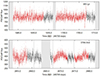 |
Fig. 1. Examples of light curves (black points) with gaps (shaded grey areas) and selected portions (red points) with a duration of 10 (upper panel) and 5 (lower panel) days for PDS analysis. |
The second step was to select the light curve portions with a duration of nd days. The empirically derived optimal value is 10. However, not all of the examined objects have such uninterrupted 10 day intervals. Therefore, we performed the analysis using nd = 5 and 10. We could use the whole light curve portion between the gaps, but we prefer to have all PDSs equivalent with the same frequency resolution and PDS point step.
To estimate the PDS, we divided each light curve portion into nsubs subsamples. For each subsample, we calculated a periodogram using the Lomb-Scargle algorithm2 (Scargle 1982). All periodograms (power3p as a function of the frequency, f) were subsequently transformed into the log-log space. Averaging of log(p) instead of p is recommended by Papadakis & Lawrence (1993). We re-binned the whole log(f) interval of the PDS with a constant frequency step of 0.1 dex. Finally, all of the log(p) points within each frequency bin were averaged. We defined an additional condition for averaging; the number of averaged periodogram points per bin must be larger than some pre-selected value defined as nmin × nsubs (nmin points from each of nsubs periodograms). If the condition is not valid, the bin should be broadened until the condition is fulfilled. This allows us to get enough points for the mean value with the standard error of the mean calculation.
The PDS frequency resolution and the lowest PDS frequency (before re-binning) are proportional to the duration of the light curve subsamples. Therefore, an empirical compromise between noise and resolution must be found. As nsubs and nmin × nsubs values, we chose 10 and 3 × 10, respectively. The high-frequency end of the periodogram was set by the Nyquist frequency.
We fitted the resulting PDSs with a broken power law model using the GNUPLOT4 software. The selected frequency range was from log(f/Hz) = −3.5 to −2.4.
3.2. Selection of positive detections
The first step was to identify systems with a PDS contaminated by other signals not associated with flickering. Superhumps and orbital periods are no longer a complication, as was described above. However, IPs like AO Psc and IGR J08390-4833 have spin frequencies of log(f/Hz) = −2.91 (van der Woerd et al. 1984) and –3.16 (Sazonov et al. 2008), respectively. This clearly affects the studied PDSs (left panel in Fig. 2). We excluded these systems from the analysis.
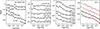 |
Fig. 2. Examples of PDSs. The black points represent PDSs with nd = 10 and black circles are for nd = 5. First (left) panel: IPs with a strong spin frequency affecting the PDS. Second panel: Example of PDSs dominated by white noise. Third panel: Example of PDSs dominated by red noise. Fourth (right) panel: Examples of PDSs of MV Lyr with broken power law fits. The upper PDS shows the case in which the fitting process did not converge on the broken power law shape. There is no fb but a straight line instead. The middle two cases represent a possible positive detection but with an fb error larger than 0.10. Apparently, the fb is not clear even if the fit converges. The lower case is an example of a positive detection with a small-enough error of the fb due to the clear broken power law shape of the PDS. Individual PDSs are offset vertically for better visualisation. |
The second step was to select objects with positive fb detections. Systems where the PDS is dominated by white (second panel of Fig. 2) or red noise (third panel of Fig. 2) did not yield any detection. More problematic are the cases in which random features or noise in the PDS can mimic the searched fb. For this reason, we selected only those PDSs for which fb is persistent and stable. This means that it must be detected at various times and with similar values. For this selection process, we relied on well-studied MV Lyr (Scaringi et al. 2012a). The detection of fb close to log(f/Hz) = −3 is unambiguous thanks to the Kepler observations. After inspecting individual PDSs from the TESS light curves, we selected only those light curve subsamples where the detected fb has an error of 0.10 or less5. Larger errors occurred in cases of clearly scattered and noisy PDSs (right panel in Fig. 2) or where the break was not obvious, making the broken power law shape is untrustworthy. Moreover, if the PDSs did not show the broken power law shape at all, the fit did not converge on such a shape, and the fb reached the end with absurd errors. This selection process yields 19 detections of fb out of 27 light curve subsamples with nd = 5, and 10 detections out of 13 light curve subsamples with nd = 10. Therefore, the fraction of positive detections, np, is 70% and 77% for nd = 5 and nd = 10, respectively. Apparently, the persistent fb in MV Lyr is not detected in all light curve subsamples, probably due to the limited capabilities of TESS, yielding more scattered PDSs compared to the Kepler results. Therefore, as positive detections in all other systems we chose cases in which the np parameter was at least 50%. However, if the total number of light curve subsamples is only two, the detection of a single fb (nm = 1) is not sufficient. Therefore, we considered a detection to be positive if at least two fb were detected (nm = 2). More strict conditions will be applied later.
3.3. Results
Figure 3 shows selected examples of PDSs with fits for objects for which we found positive detections. Figure 4 shows measured fb with errors for all positive detections. Both nd of 5 and 10 are shown. As was previously mentioned, the nd = 5 case is more scattered than nd = 10. Therefore, we rely on nd = 10 if possible. Only TT Ari and V704 And does not have long-enough uninterrupted light curve portions and only the nd = 5 cases are shown. To judge whether the scatter of measurements is acceptable or not, we again used the well-studied MV Lyr as a benchmark. The nd = 10 measurements scatter between values log(f/Hz) = −2.79 and −3.09. All points are randomly redistributed around the value of log(f/Hz) = −2.9, and only the last point (measurement 10) deviates slightly towards higher frequencies. We investigated the long-term AAVSO light curve and concluded that this measurement was made during a transition from a high state to a low one (Fig. 5). Dobrotka et al. (2020) show that the fb increases during such transition, and therefore the deviation towards higher frequencies is natural. Since we need stationary data, we excluded this measurement from our analysis. The last observation but one was not made during the ‘standard’ high state before day MJD = 2400, but apparently occurred during a stable plateau. The brightness differs from that of all other observations, but since it is stabilised, the disc probably has all the physical characteristics of the standard high state. Finally, the measured fb shows no suspicious deviation. All other TESS observations were taken during the standard high state. Therefore, as the measurement scatter we have taken the frequency interval from log(f/Hz) = −2.85 to −3.09 (shaded grey area in Fig. 4). Based on more precise measurements using the superior spacecraft Kepler, this scatter is natural and represents the well-known fb at approximately log(f/Hz) = −3 (f2 in Fig. 1 from Dobrotka et al. 2020).
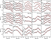 |
Fig. 3. Examples of PDSs for individual systems with broken power law fits (red lines). The black points represent PDSs with nd = 10 and the black circles are for nd = 5. Individual PDSs are offset vertically for better visualisation. |
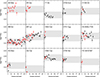 |
Fig. 4. Measurements of fb where conditions for positive detection were satisfied (see text for details). The red and black points represent the nd = 10 and 5 case, respectively. The shaded grey area is the natural scatter based on MV Lyr case. The BB Dor case is not fully displayed for clarity, but the hidden measurements have the same scatter as the ones shown (compared to the shaded grey area). |
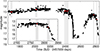 |
Fig. 5. AAVSO light curve of MV Lyr with observation intervals of TESS marked by shaded grey areas. The inset panel shows in detail the two most recent TESS observations falling before and at the beginning of the decline from the high optical state. The red points are the mean brightness of the AAVSO data during the TESS observations. |
In Fig. 4, as a priority we have taken and described the nd = 10 case. This was only not possible for TT Ari and V704 And, for which we relied on nd = 5 data. All of the measurements lie within the shaded grey area, except for AH Men and, as has already been discussed, MV Lyr. AH Men falls very well to the scatter interval too except for one single point (the 11th measurement). The AAVSO light curve is not covered enough for us to judge whether the system experienced a similar brightness transition to MV Lyr. Anyhow, all of the other measurements are robust; therefore, we excluded the deviated point from all subsequent analysis and discussions. All of the measured and selected fb values displayed in Fig. 4 are summarised in Tables A.1 and A.2.
To test the hypothesis from Dobrotka et al. (2020) regarding the prevalence of fb at approximately log(fb/Hz) = −3, we calculated a histogram representing the statistical distribution of measured fb values from log(fb/Hz) = −3.4 to −2.56. For this purpose, we used weighted averages of measured fb values using nd = 10 preferentially. This averages are summarised in Table 1. The corresponding histograms with eight bins7 are depicted in the upper panels of Fig. 6.
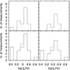 |
Fig. 6. Histograms of weighted means (number of measurements) of fb of individual systems. Left panels: Systems with a minimum number of selected fb equal to two (AH Men, BB Dor, KQ Mon, KR Aur, MV Lyr, QU Car, TT Ari, V504 Cen, V592 Cas, V704 And, V751 Cyg, V795 Her, V1193 Ori, HS 0506+7725, and TIC 92167387). Right panels: Systems with a minimum number of selected fb equal to five (AH Men, BB Dor, KR Aur, MV Lyr, TT Ari, V592 Cas, V751 Cyg, V795 Her, V1193 Ori, and HS 0506+7725). Upper panels: Measurements from this paper. Lower panels: Same as upper panels, but with added measurements from other works. The red line represents the uncertain V4743 Sgr case. |
First, we show all systems from Fig. 4 (upper left panel). This case is based on systems with a minimum number of selected fb measurements equal to two. Such a number is too low to judge whether the fb is stable or not. A larger criterion would be better to increase the confidence of the histogram. However, the larger this criterion, the lower the number of systems in the histogram. This is at the expense of the histogram resolution. Nevertheless, we show also a more conservative case with a minimum number of fb measurements equal to five. Focusing primarily on the nd = 10 condition, this excludes KQ Mon, QU Car, TT Ari, V504 Cen, V592 Cas, V704 And, V751 Cyg, V795 Her, V1193 Ori, and TIC 92167387. If the nd = 10 case did not satisfy the condition of minimum detections of five, we used nd = 5 case instead. This brings back TT Ari, V592 Cas, V751 Cyg, V795 Her, and V1193 Ori. The corresponding histogram is in the upper right panel of Fig. 6.
4. Discussion
We investigated the optical flickering of CVs in a high optical state. For this purpose, we selected nova-like systems observed by TESS satellite. We searched for the break frequency, fb, in corresponding PDSs. The goal was to increase the low number (just five) of detections in Dobrotka et al. (2020). We found 13 new (15 in total) systems with positive detections of fb. The histograms in Fig. 6 depict the resulting statistics.
4.1. Power density spectra break frequency
Dobrotka et al. (2020) formulated a hypothesis that CVs in a high state have a preferable fb close to log(f/Hz) = −3. Fig. 6 supports this possibility. Apparently, the measurements cluster and culminate close to log(f/Hz) = −3. The upper panels show the detections from this work, while the lower panels depict the statistics after including additional MV Lyr8, KR Aur, V1504 Cyg, V344 Lyr, and V4743 Sgr values from Table 2 of Dobrotka et al. (2020). UU Aqr was not added because it is outside of the studied frequency range from log(f/Hz) = −3.4 to −2.5.
The only problematic object is V4743 Sgr, identified as an IP with a magnetic WD (Ness et al. 2003; Kang et al. 2006). Such magnetic CVs have truncated discs with the inner disc edge responsible for the fb observed very close to log(f/Hz) ≃ −3 or higher (Revnivtsev et al. 2010; Semena et al. 2014). Usually, these fb are close to the spin frequency of the WD. This is also the case for V4743 Sgr (Dobrotka et al. 2021). This means that the measured fb can be of different origin than the studied flickering in non-magnetic CVs like in this work. However, all IPs have a disc in a low state (Hameury & Lasota 2017), while Dobrotka et al. (2021) suggests that the disc in V4743 Sgr is in a high state, making this IP different from standard IPs. It is a post-nova. Therefore, it is possible that the measured fb has a different origin than in standard IPs, and that it represents the studied flickering. But since this is only a possibility, we mark it as a red line in Fig. 6.
The histogram in Fig. 6 is divided into eight equally spaced bins with a slightly narrower frequency extension than the one used in Dobrotka et al. (2020). This different spacing with a slightly better resolution (0.113 vs. 0.144) allows us to better identify the fb, which is between log(f/Hz) = −2.95 and –2.84. The question is whether the observed dominant bin in the histogram represents a preferred or most frequent value, or whether it is just a random feature of a uniform distribution. Dobrotka et al. (2021) simulated such a histogram with a uniform distribution and concluded that 31% of simulations yield at least one bin with a height equal to or larger than that of the dominant bin in their Fig. 11. This means that the statement that the dominant bin represents a preferred frequency has a confidence of only 69%. Adding the V4743 Sgr case, this confidence increases to 91%.
With the new histogram in Fig. 6, we see that the V4743 Sgr case does not fall into the dominant bin, and therefore does not increase the estimated confidence. We performed the same simulations as Dobrotka et al. (2021), and after one million repetitions, we got confidences of 99 and 96% using only TESS detections from this work for a minimum number of two and five fb measurements (upper panels of Fig. 6), respectively. Adding all other measurements except for V4743 Sgr (lower panels of Fig. 6) yields confidences of 96 and 85%. Finally, adding the questionable post-nova too yields values of 95 and 81%.
Apparently, the worst case is 81%, but excluding the uncertain V4743 Sgr it is 85%. Therefore, we got a significant increase in confidence compared to the original 69%, but still not enough for a definite conclusion, unless we want to rely on the less conservative case with a minimum number of fb measurements of two. Nevertheless, we must be cautious in adding measurements from different instruments. If TESS is able to detect only the dominant fb in MV Lyr, and Kepler is able to see fainter PDS structures, we may discuss the dominant value close to log(f/Hz) = −3, but it may be confusing to judge the statistical significance of the presence of other frequencies detected by Kepler only. Therefore, it is best to rely on measurements from this work based on TESS observations only. In such a case, the more conservative approach yields a confidence of 96%. This is already high enough to conclude that nova-like CVs very probably have a preferred fb between log(f/Hz) = −2.95 and –2.84. Whether it is really a kind of preferred value or just a maximum in a smooth fb distribution is not yet known due to the low number of fb measurements.
4.2. Dependence on physical parameters
The next step is to understand the physical meaning of such a preferred value or distribution maximum. The best way is to search for a correlation of the fb with basic physical parameters. Comparing fb values with orbital periods did not yield any correlation. The data show just a scattered cloud of points. This is not surprising because the flickering in CVs and related objects is usually associated with the accretion disc and especially its inner regions (Bruch 1992, 1996; Zamanov & Bruch 1998; Bruch 2000; Baptista & Bortoletto 2004; Scaringi 2014), while the orbital period is more typically associated with the secondary star characteristics (Smith & Dhillon 1998).
The inner disc region potentially connected to the flickering is the inner disc edge. Balman & Revnivtsev (2012) suggests that the fb represents the Keplerian frequency at this inner disc edge. If true, the fb should be higher in the high state compared to the low state. However, the opposite is observed in the case of the nova-like MV Lyr (Dobrotka et al. 2020). Nova-likes in a high state are similar to dwarf novae in outburst where the inner disc extends down to the WD surface or close to it. Once the CV changes states, the disc starts to be truncated and the Keplerian frequency should decrease during the transition. The opposite was observed in the transition of MV Lyr detected by the Kepler spacecraft. The dominant fb at log(f/Hz) = −3 increased together with another one or two adjacent PDS components. Anyhow, this does not tell us anything about the preference of any fb value. Even if the fb is generated by the inner disc edge, the preference would suggest some preferred inner disc radius. It is hard to test such a statement because measurements of the inner disc radii are rare.
An alternative interpretation is the sandwich model with an inner hot corona. Based on the accretion fluctuation propagation model, an accretion inhomogeneity forms somewhere in the disc and propagates inwards. Such a fluctuation follows the local physical conditions and the local viscous timescale. The further away from the centre that such a fluctuation is generated, the larger the corresponding timescale. If the fluctuations are generated in the inner corona, the outer radius of such geometrically thick disc determines the largest timescale of the fluctuations. Therefore, the larger the corona’s outer radius, the lower the fb (Fig. 3 in Scaringi 2014). This may explain the increase in fb during the transition of MV Lyr from a high state to a low one. If ṁacc decreases during such a transition, the energy generation decreases too. Lower energy yields lower matter evaporation and the corona may shrink. As a consequence, this shrinking generates an increase in fb. Similar reasoning may be applied when considering mass of the central WD, mWD. A larger mWD generates a deeper potential well. This results in higher temperatures of the inner disc and the corona can be evaporated to further distances from the centre. A more radially extended corona such as this should generate a lower fb.
To test the mWD scenario, we need to collect the mass measurements. In the case of nova-likes, this is not easy because the accretion rate is too high to allow for the detection of a WD, even at UV wavelengths. An accretion disc model or a combination of it with a WD model can be used instead. AH Men was studied using IUE spectroscopy (Gänsicke & Koester 1999). Unfortunately, the determined mWD is not unambiguous due to conflicts with distance constraints. The disc modelling yields values of 0.35 and 0.55 M⊙. We used a mean value of 0.45 ± 0.10 M⊙. Godon et al. (2008) studied FUSE spectra of BB Dor and disc modelling derived a mWD of 0.8 M⊙. KQ Mon mWD was determined by Wolfe et al. (2013) using archival IUE spectra. Its value from disc modelling is estimated as 0.6 M⊙. KR Aur has several mWD estimates. Shafter (1983) used a somewhat controversial method (as was stated by the authors) using radial velocities and estimated a value of 0.7 M⊙ using spectra from ground observations. Mizusawa et al. (2010) used IUE spectra and derived a slightly lower mass of 0.6 M⊙ using a combination of disc and WD models. These two estimates agree well with another value of 0.59 ± 0.17 M⊙ from the Ritter & Kolb (2003) catalogue. Most recently, Rodríguez-Gil et al. (2020) used GTC spectra during a low state, during which the WD is dominant and well seen. They derived a quite different mass from the previous estimates with a value of  M⊙. For MV Lyr, Hoard et al. (2004) derived a mass of 0.73 ± 0.10 M⊙ from FUSE spectroscopy using a combined WD + disc model. The system was observed in a low state, and therefore the spectrum was dominated by the WD features. The mWD of QU Car was determined using combined FUSE, HST, and IUE spectra (Linnell et al. 2008). A non-standard accretion disc model yields mWD between 0.6 and 1.2 M⊙. We have used a mean value of 0.9 ± 0.3 M⊙. mWD in TT Ari can be estimated as 0.57 M⊙ using spectra from ground observations and applying a disc plus an additional black body model (Belyakov et al. 2010). Huber et al. (1998) used photometric and spectroscopic data to study the system parameters of V592 Cas. The authors acknowledge that the method they used is criticised by several other authors9. Their estimated mWD is
  M⊙. We take 1.4 M⊙ as an upper limit due to the Chandrasekhar limit. Finally, the WD of V795 Her has a mass of approximately 0.8 M⊙ by Mizusawa et al. (2010) using IUE spectra and the disc + WD atmosphere model. All of the values are summarised in Table. 2.
Used system parameters.
The upper panel of Fig. 7 shows the correlation between mWD and fb of the systems mentioned. The first view is rather uncertain. Ignoring the problematic measurements shown by the red colour, mainly the V592 Cas case, the situation is clearer. Only the too-scattered KR Aur complicates the judgement. Without the highest mWD estimate, there is a tendency to see the anticipated correlation. fb decreases with increasing mWD. The scatter of points is relatively large, but this is natural because determination of mWD is very uncertain and is usually done with large errors. Therefore, we cannot definitely conclude whether the correlation is real or if the redistribution of points is just random. There are three ways of answering whether the correlation is real. We should either refine or revise mWD of KR Aur and QU Car, increase the number of measured fb for systems with known mWD, or get fb measurements for CVs with high mWD (above 1 M⊙) to populate the upper right region of upper panel of Fig. 7.
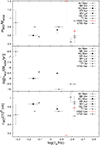 |
Fig. 7. mWD (upper panel), ṁacc (middle panel), and rWD (bottom panel) vs fb from Table 1. The red colour represents uncertain measurements. |
If fb is really correlated with mWD, the preferred value between log(f/Hz) = −2.95 and −2.84 suggests the existence of a preferred mWD. Zorotovic et al. (2011) studied the mWD distribution in CVs and their Fig. 7 shows a maximum at 0.8 M⊙. This can represent the preferred value mentioned, and in such case it would be just a maximum of an otherwise smooth distribution. The best way to check whether the maximum in fb represents the observed maximum in mWD is to fit the data in the upper panel of Fig. 7 with a linear function. Unfortunately, the fits have errors that are too large, mainly for the first coefficient defining the correlation or anticorrelation10. Moreover, Dobrotka et al. (2020) mentioned that three possible groups of fb could be present, but due to the very low number of measurements it is not possible to confirm or reject this statement. Wijnen et al. (2015) theoretically studied the mWD distribution and found three local maxima in simulated histograms. Therefore, the possibility that the fb distribution has a more complicated structure has a physical meaning. However, the histogram in Dobrotka et al. (2020) was constructed using the well-studied MV Lyr, V1504 Cyg, and V344 Lyr cases in which multi-component PDSs were found. Therefore, such a histogram is contaminated by multiple measurements for one single mWD. In such a case, the multiple structure of the histogram rather represents different sources of the fast variability with different fb, and the potential correlation between mWD and fb would only be for some specific fb. MV Lyr and V1504 Cyg PDS show one dominant break and all of the other features are relatively weak. This dominant fb seen in TESS data can be correlated with mWD.
mWD and its deeper potential well is not the only reason for the higher temperature of the disc. Larger increased energy generation and subsequently stronger evaporation of matter into the corona can be produced by higher ṁacc too. The middle panel of Fig. 7 shows this case. We used values from Table. 2. It seems that fb decreases with increasing ṁacc. However, this correlation is based mainly on one single deviated point representing QU Car. Otherwise, the points do not show any significant correlation. Finally, both mWD and ṁacc together can play a role. The higher potential well of a massive WD and higher ṁacc can generate a larger radius of an evaporated corona. For a detailed investigation, many more systems need to be studied.
The confirmation of the corona scenario via such a correlation between fb and the system parameters has a very important consequence. As was mentioned in the introduction, the ratio of X-ray to optical luminosity is of the order of 0.1 (Dobrotka et al. 2020) or even 0.01–0.001 (Balman et al. 2014). The question, then, is how it is possible that X-rays are able to generate the observed optical radiation. Scaringi (2014) proposed reprocessing, which apparently cannot work. An alternative must be searched for elsewhere. The variability can be generated by the corona. The reprocessing of X-rays from the corona generates only a faint response. Such a response can take the form of the small side lobes found in the shot profile by Dobrotka et al. (2019). The shot profile has another dominant feature, the central spike. This has too large an amplitude to be explicable by the reprocessing. It must originate directly from the central geometrically thin disc. The variability in the corona is generated by the propagation of accretion fluctuations (Scaringi 2014). If these fluctuations somehow influence the underlying geometrically thin disc flow, the timescale of the optical flickering can have the same timescales. Such an influence can be re-condensation of the corona back into the thin disc (Meyer et al. 2007). If the corona generates the log(f/Hz) = −3 variability via mass accretion fluctuations, these fluctuations re-condensate and propagate in the thin disc. This can generate optical variability with the same frequency.
Finally, for authors identifying the boundary layer as the source of the flickering, it is important to relate fb with the WD radius, rWD. We display such a case in the bottom panel of Fig. 7. For the WD radius, we used the relation by Nauenberg (1972); hence, the figure looks similar to the mWD versus fb case. Since the relation between mWD and rWD is not linear, the increase in rWD with increasing fb is accentuated, yielding better linear fits than in the mWD case. While the fits of mWD versus fb did not yield a definite slope character (rising or declining) due to large parameter errors, the rWD case is much better with a clearly positive slope11. However, the derivation of rWD is not independent from the derivation of mWD, and the ‘better’ fits are just results of the non-linear transformation. Therefore, we cannot conclude any fit ‘superiority’, and the character of the data is still uncertain and more measurements are needed, as was concluded for mWD.
4.3. Detection versus non-detection of fb
An indirect indication that the central disc region is the source of the studied flickering can be gotten from the discussion about the detection versus non-detection of fb. The first idea is that the detection depends on the brightness of the binary. This is valid for systems with dominant white noise. Those systems have the lowest mean fluxes; therefore, Poisson noise dominates the corresponding PDSs. However, all other systems with fb detection or a PDS dominated by red noise are equally distributed with no preferred fluxes except for the bright TT Ari and QU Car. These two systems have significantly higher fluxes, and fb detection. But only two systems with a specific flux does not say anything about any flux preference.
Apparently, the reason for detection versus non-detection must be searched for elsewhere. The localisation of the flickering source could be the clue. If the source is the inner geometrically thin disc, either radiating directly or reprocessing X-rays from the central corona, it must be seen. This can be problematic in eclipsing systems or in systems with high inclination. In such conditions, the central disc can be obscured by the outer disc edge. Investigating the inclinations (Table. 2) of systems with detected fb, we see that all have values below 75°. Taking the lower estimate of KQ Mon, the inclinations are below 60°. On the other hand, systems with red noise PDSs are eclipsing like AY Psc (Szkody et al. 1989), BH Lyn (Andronov 1986; Richter 1989; Andronov et al. 1989), and NSV 1907 (Hümmerich et al. 2017), or have higher inclinations (Table. 2). Clearly, the inclination in red noise systems is higher than 65°. Therefore, there is a possible overlap of inclinations only in the case of KQ Mon with the low end of red noise systems. Otherwise, the inclinations are very different, implying that fb is seen only in low-inclination systems.
Another reason for missing fb that is also related to the inner disc regions is the IP nature of the system. In these CVs, the central disc is truncated, and therefore missing, due to the magnetic field of the WD. This is the case, for example, for RX J2133.7+5107 (Bonnet-Bidaud et al. 2006), where we see only red noise with a clear spin frequency seen as one significantly deviated PDS bin. The PDS is not deformed like the examples in the left panel of Fig. 2; therefore, the red noise character is clear. V533 Her is a similar case with no fb detection and is an IP candidate (Worpel et al. 2020). The PDSs have an ambiguous shape with a not-always-present (variable from observation to observation) PDS structure near the potential spin frequency of log(f/Hz) = −3.15 (Rodríguez-Gil & Martínez-Pais 2002). We should exclude this binary from analysis, like we did for the examples in the left panel of Fig. 2, but since the spin frequency is not obvious we have kept it. Anyhow, we did not get any fb detection; therefore, this case is also consistent with the missing inner disc region in IPs.
Finally, it is worth discussing the CP Pup case. The PDS is neither pure red noise nor white noise. Red noise is clear up to approximately log(f/Hz) = −2.7 to −3, and a white noise plateau continues for higher frequencies. Szkody & Feinswog (1988) reported an inclination of 32° or 37°. Based on our inclination assumption, such a system should show a clear fb. However, the authors reported a potential WD mass of only 0.18 M⊙ for a mass ratio of 1. A similar potential low mass of 0.12 M⊙ or 0.27 M⊙ was concluded also in Duerbeck et al. (1987). In the case of the existing relation between fb and mWD and based on the characteristics of Fig. 7, the potential fb (if present) can be outside of the studied frequency range for such low mWD or can be hidden in the high-frequency part of the PDS that is dominated by Poisson white noise. Therefore, CP Pup does not contradict the low-inclination criterion for fb detection, and thanks to its probable low mWD it is a very suitable object for testing any relation between fb and mWD.
5. Summary and conclusions
Dobrotka et al. (2020) summarise characteristic fb of the flickering in CVs. The authors found that it is very probable that the PDSs of these systems have a preferred value close to log(f/Hz) = −3 but only in a high optical state. However, the probability of such a conclusion is only 69% (Dobrotka et al. 2021). It is still possible that the resulting histogram of measured fb is the result of a random distribution. More measurements are needed to improve the statistics.
We selected nova-like CVs observed by TESS and we searched for fb in PDSs. These systems spend the majority of their lifetimes in a high optical state. We selected uninterrupted light curve portions with durations of 5 and 10 days. We divided these portions into ten equally spaced subsamples and we calculated the mean PDSs. We focused our search on the frequency interval from log(f/Hz) = −3.5 to −2.4, looking for the mentioned mHz fb.
We found 15 positive detections, and the resulting histogram shows the searched-for preferred value (maximum) close to the log(f/Hz) = −3. Thanks to the higher number of measurements compared to Dobrotka et al. (2020), we refined this value to the interval from log(f/Hz) = −2.95 to −2.84. The probability that this histogram maximum is not the result of just a random distribution is 96% in the more conservative case. Apparently, this is much larger than the previous value of 69%. Moreover, it is possible that the fb is correlated with WD mass; the higher the mass, the lower the fb. However, such a statement has only low confidence due to the still-low number of studied systems with a known WD mass and needs to be confirmed by further work. We need to increase the number of systems where the fb is detected, and/or we should focus on systems with lower values close to log(f/Hz) = −3.5 to populate the empty region of the WD mass versus fb parametric space.
As was mentioned, only 15 systems show a clear fb detection. All other objects have a PDS dominated by white or red noise. While the white noise is the result of low brightness, the red noise is seen only in high-inclination systems.
Both the inclination dependence and the possible correlation between fb and WD mass points to inner disc regions being the source of the detected fb. This region is not well seen in high-inclination systems and is completely obscured in eclipsing CVs. The potential correlation between fb and WD mass could be explained by the inner hot corona being a source of fb that is more radially extended for more massive WDs.
Using Python Lightkurve library; https://lightkurve.github.io/lightkurve/.
We used python’s package Astropy (Astropy Collaboration 2013, 2018, 2022).
We use power normalized by the total variance according to Horne & Baliunas (1986). Since the normalization does not affect the shape of the PDS, this has no importance in our case.
Since this error limit is more or less approximate and empirically estimated, we took all values rounded to 0.10, therefore up to 0.10499... This allowed us to get five additional measurements. This was useful mainly in AH Men case where it helped to fulfill the np = 50% condition.
Since the fit is performed on interval from log(fb/Hz) = −3.5 to −2.4, the break frequency cannot fall to the boundaries.
Comparable to Fig. 11 in Dobrotka et al. (2020).
For MV Lyr we added only values of log(f/Hz) = −3.3 and −2.5, because fb close to log(f/Hz) = −3 was used from this work.
It is the same method as used for KR Aur by Shafter (1983) where the authors acknowledge the problematic aspect.
Using all black data, we got mWD = ( − 0.07 ± 0.84)log(fb)+(−0.26 ± 0.28) M⊙, while excluding the KR Aur case because of an overly scattered mass estimate we got mWD = ( − 0.81 ± 1.05)log(fb)+(−0.49 ± 0.34) M⊙. We did not use mWD errors, since they are not known for every system. Adding at least 0.1 M⊙ as error, the fit is even worse; the relative errors are larger or the direction turns positive in the case of all black data.
Using all black data, we got rWD = (1.47 ± 0.71)log(fb)+(0.23 ± 0.24) 109 cm, while excluding the KR Aur case because of an overly scattered mass estimate we got rWD = (2.12 ± 0.91)log(fb)+(0.43 ± 0.30) 109 cm. Like in the mWD case, we did not use errors because they are not known for every system, and therefore the fit is just rough and orientational.
Acknowledgments
This work was supported by the Slovak grant VEGA 1/0576/24. We acknowledge with thanks the variable star observations from the AAVSO International Database contributed by observers worldwide and used in this research.
References
- Andronov, I. L. 1986, Astronomicheskij Tsirkulyar, 1418, 1 [NASA ADS] [Google Scholar]
- Andronov, I. L., Kimeridze, G. N., Richter, G. A., & Smykov, V. P. 1989, IBVS, 3388, 1 [NASA ADS] [Google Scholar]
- Arévalo, P., & Uttley, P. 2006, MNRAS, 367, 801 [Google Scholar]
- Astropy Collaboration (Robitaille, T. P., et al.) 2013, A&A, 558, A33 [NASA ADS] [CrossRef] [EDP Sciences] [Google Scholar]
- Astropy Collaboration (Price-Whelan, A. M., et al.) 2018, AJ, 156, 123 [Google Scholar]
- Astropy Collaboration (Price-Whelan, A. M., et al.) 2022, ApJ, 935, 167 [NASA ADS] [CrossRef] [Google Scholar]
- Balman, Ş., & Revnivtsev, M. 2012, A&A, 546, A112 [NASA ADS] [CrossRef] [EDP Sciences] [Google Scholar]
- Balman, Ş., Godon, P., & Sion, E. M. 2014, ApJ, 794, 84 [NASA ADS] [CrossRef] [Google Scholar]
- Baptista, R., & Bortoletto, A. 2004, AJ, 128, 411 [NASA ADS] [CrossRef] [Google Scholar]
- Baptista, R., & Bortoletto, A. 2008, ApJ, 676, 1240 [Google Scholar]
- Belyakov, K. V., Suleimanov, V. F., Nikolaeva, E. A., & Borisov, N. V. 2010, AIP Conf. Ser., 1273, 342 [NASA ADS] [Google Scholar]
- Bonnet-Bidaud, J. M., Mouchet, M., de Martino, D., Silvotti, R., & Motch, C. 2006, A&A, 445, 1037 [NASA ADS] [CrossRef] [EDP Sciences] [Google Scholar]
- Bruch, A. 1992, A&A, 266, 237 [NASA ADS] [Google Scholar]
- Bruch, A. 1996, A&A, 312, 97 [NASA ADS] [Google Scholar]
- Bruch, A. 2000, A&A, 359, 998 [NASA ADS] [Google Scholar]
- Bruch, A. 2015, A&A, 579, A50 [NASA ADS] [CrossRef] [EDP Sciences] [Google Scholar]
- Bruch, A. 2022, MNRAS, 514, 4718 [NASA ADS] [CrossRef] [Google Scholar]
- Bruch, A. 2023a, MNRAS, 519, 352 [Google Scholar]
- Bruch, A. 2023b, MNRAS, 525, 1953 [CrossRef] [Google Scholar]
- Dobrotka, A., & Ness, J.-U. 2015, MNRAS, 451, 2851 [Google Scholar]
- Dobrotka, A., Mineshige, S., & Ness, J.-U. 2014, MNRAS, 438, 1714 [Google Scholar]
- Dobrotka, A., Ness, J.-U., & Bajčičáková, I. 2016, MNRAS, 460, 458 [Google Scholar]
- Dobrotka, A., Ness, J.-U., Mineshige, S., & Nucita, A. A. 2017, MNRAS, 468, 1183 [Google Scholar]
- Dobrotka, A., Negoro, H., & Mineshige, S. 2019, A&A, 631, A134 [NASA ADS] [CrossRef] [EDP Sciences] [Google Scholar]
- Dobrotka, A., Negoro, H., & Konopka, P. 2020, A&A, 641, A55 [EDP Sciences] [Google Scholar]
- Dobrotka, A., Orio, M., Benka, D., & Vanderburg, A. 2021, A&A, 649, A67 [NASA ADS] [CrossRef] [EDP Sciences] [Google Scholar]
- Duerbeck, H. W., Seitter, W. C., & Duemmler, R. 1987, MNRAS, 229, 653 [NASA ADS] [Google Scholar]
- Gänsicke, B. T., & Koester, D. 1999, A&A, 346, 151 [Google Scholar]
- Godon, P., Sion, E. M., Barrett, P. E., Szkody, P., & Schlegel, E. M. 2008, ApJ, 687, 532 [NASA ADS] [CrossRef] [Google Scholar]
- Hameury, J. M., & Lasota, J. P. 2017, A&A, 602, A102 [Google Scholar]
- Hoard, D. W., Linnell, A. P., Szkody, P., et al. 2004, ApJ, 604, 346 [NASA ADS] [CrossRef] [Google Scholar]
- Honeycutt, R. K., & Kafka, S. 2004, AJ, 128, 1279 [NASA ADS] [CrossRef] [Google Scholar]
- Horne, J. H., & Baliunas, S. L. 1986, ApJ, 302, 757 [Google Scholar]
- Hōshi, R. 1979, Prog. Theor. Phys., 61, 1307 [CrossRef] [Google Scholar]
- Huber, M. E., Howell, S. B., Ciardi, D. R., & Fried, R. 1998, PASP, 110, 784 [NASA ADS] [CrossRef] [Google Scholar]
- Hümmerich, S., Gröbel, R., Hambsch, F.-J., et al. 2017, New Astron., 50, 30 [CrossRef] [Google Scholar]
- Kang, T. W., Retter, A., Liu, A., & Richards, M. 2006, AJ, 132, 608 [Google Scholar]
- Kato, T., Ishioka, R., & Uemura, M. 2002, PASJ, 54, 1033 [Google Scholar]
- Kotov, O., Churazov, E., & Gilfanov, M. 2001, MNRAS, 327, 799 [Google Scholar]
- Linnell, A. P., Szkody, P., Gänsicke, B., et al. 2005, ApJ, 624, 923 [NASA ADS] [CrossRef] [Google Scholar]
- Linnell, A. P., Godon, P., Hubeny, I., et al. 2008, ApJ, 676, 1226 [NASA ADS] [CrossRef] [Google Scholar]
- Lyubarskii, Y. E. 1997, MNRAS, 292, 679 [Google Scholar]
- Meyer, F., & Meyer-Hofmeister, E. 1981, A&A, 104, L10 [NASA ADS] [Google Scholar]
- Meyer, F., & Meyer-Hofmeister, E. 1994, A&A, 288, 175 [NASA ADS] [Google Scholar]
- Meyer, F., Liu, B. F., & Meyer-Hofmeister, E. 2007, A&A, 463, 1 [NASA ADS] [CrossRef] [EDP Sciences] [Google Scholar]
- Mizusawa, T., Merritt, J., Ballouz, R.-L., et al. 2010, PASP, 122, 299 [NASA ADS] [CrossRef] [Google Scholar]
- Nauenberg, M. 1972, ApJ, 175, 417 [NASA ADS] [CrossRef] [Google Scholar]
- Ness, J., Starrfield, S., Burwitz, V., et al. 2003, ApJ, 594, L127 [Google Scholar]
- Osaki, Y. 1974, PASJ, 26, 429 [NASA ADS] [Google Scholar]
- Papadakis, I. E., & Lawrence, A. 1993, MNRAS, 261, 612 [Google Scholar]
- Revnivtsev, M., Burenin, R., Bikmaev, I., et al. 2010, A&A, 513, A63 [NASA ADS] [CrossRef] [EDP Sciences] [Google Scholar]
- Richter, G. A. 1989, IBVS, 3287, 1 [NASA ADS] [Google Scholar]
- Ritter, H., & Kolb, U. 2003, A&A, 404, 301 [NASA ADS] [CrossRef] [EDP Sciences] [Google Scholar]
- Rodríguez-Gil, P., & Martínez-Pais, I. G. 2002, MNRAS, 337, 209 [Google Scholar]
- Rodríguez-Gil, P., Shahbaz, T., Torres, M. A. P., et al. 2020, MNRAS, 494, 425 [CrossRef] [Google Scholar]
- Sazonov, S., Revnivtsev, M., Burenin, R., et al. 2008, A&A, 487, 509 [NASA ADS] [CrossRef] [EDP Sciences] [Google Scholar]
- Scargle, J. D. 1982, ApJ, 263, 835 [Google Scholar]
- Scaringi, S. 2014, MNRAS, 438, 1233 [Google Scholar]
- Scaringi, S., Körding, E., Uttley, P., et al. 2012a, MNRAS, 427, 3396 [Google Scholar]
- Scaringi, S., Körding, E., Uttley, P., et al. 2012b, MNRAS, 421, 2854 [Google Scholar]
- Scaringi, S., Körding, E., Groot, P. J., et al. 2013, MNRAS, 431, 2535 [Google Scholar]
- Schreiber, M. R., Hameury, J. M., & Lasota, J. P. 2003, A&A, 410, 239 [NASA ADS] [CrossRef] [EDP Sciences] [Google Scholar]
- Semena, A. N., Revnivtsev, M. G., Buckley, D. A. H., et al. 2014, MNRAS, 442, 1123 [Google Scholar]
- Shafter, A. W. 1983, ApJ, 267, 222 [NASA ADS] [CrossRef] [Google Scholar]
- Smith, D. A., & Dhillon, V. S. 1998, MNRAS, 301, 767 [NASA ADS] [CrossRef] [Google Scholar]
- Szkody, P., & Feinswog, L. 1988, ApJ, 334, 422 [NASA ADS] [CrossRef] [Google Scholar]
- Szkody, P., Howell, S. B., Mateo, M., & Kreidl, T. J. 1989, PASP, 101, 899 [NASA ADS] [CrossRef] [Google Scholar]
- van der Woerd, H., de Kool, M., & van Paradijs, J. 1984, A&A, 131, 137 [NASA ADS] [Google Scholar]
- Van de Sande, M., Scaringi, S., & Knigge, C. 2015, MNRAS, 448, 2430 [Google Scholar]
- Warner, B. 1995, Camb. Astrophys. Ser., 28 [Google Scholar]
- Wijnen, T. P. G., Zorotovic, M., & Schreiber, M. R. 2015, A&A, 577, A143 [NASA ADS] [CrossRef] [EDP Sciences] [Google Scholar]
- Wolfe, A., Sion, E. M., & Bond, H. E. 2013, AJ, 145, 168 [NASA ADS] [CrossRef] [Google Scholar]
- Worpel, H., Schwope, A. D., Traulsen, I., Mukai, K., & Ok, S. 2020, A&A, 639, A17 [NASA ADS] [CrossRef] [EDP Sciences] [Google Scholar]
- Zamanov, R. K., & Bruch, A. 1998, A&A, 338, 988 [NASA ADS] [Google Scholar]
- Zorotovic, M., Schreiber, M. R., & Gänsicke, B. T. 2011, A&A, 536, A42 [NASA ADS] [CrossRef] [EDP Sciences] [Google Scholar]
Appendix A: Additional tables
Tables A.1 and A.2 show all selected fb values for nd = 10 and nd = 5, respectively.
Selected fb for systems with positive detection using nd = 10.
Same as Table A.1 but for nd = 5.
All Tables
All Figures
|
Fig. 1. Examples of light curves (black points) with gaps (shaded grey areas) and selected portions (red points) with a duration of 10 (upper panel) and 5 (lower panel) days for PDS analysis. |
| In the text | |
|
Fig. 2. Examples of PDSs. The black points represent PDSs with nd = 10 and black circles are for nd = 5. First (left) panel: IPs with a strong spin frequency affecting the PDS. Second panel: Example of PDSs dominated by white noise. Third panel: Example of PDSs dominated by red noise. Fourth (right) panel: Examples of PDSs of MV Lyr with broken power law fits. The upper PDS shows the case in which the fitting process did not converge on the broken power law shape. There is no fb but a straight line instead. The middle two cases represent a possible positive detection but with an fb error larger than 0.10. Apparently, the fb is not clear even if the fit converges. The lower case is an example of a positive detection with a small-enough error of the fb due to the clear broken power law shape of the PDS. Individual PDSs are offset vertically for better visualisation. |
| In the text | |
|
Fig. 3. Examples of PDSs for individual systems with broken power law fits (red lines). The black points represent PDSs with nd = 10 and the black circles are for nd = 5. Individual PDSs are offset vertically for better visualisation. |
| In the text | |
|
Fig. 4. Measurements of fb where conditions for positive detection were satisfied (see text for details). The red and black points represent the nd = 10 and 5 case, respectively. The shaded grey area is the natural scatter based on MV Lyr case. The BB Dor case is not fully displayed for clarity, but the hidden measurements have the same scatter as the ones shown (compared to the shaded grey area). |
| In the text | |
|
Fig. 5. AAVSO light curve of MV Lyr with observation intervals of TESS marked by shaded grey areas. The inset panel shows in detail the two most recent TESS observations falling before and at the beginning of the decline from the high optical state. The red points are the mean brightness of the AAVSO data during the TESS observations. |
| In the text | |
|
Fig. 6. Histograms of weighted means (number of measurements) of fb of individual systems. Left panels: Systems with a minimum number of selected fb equal to two (AH Men, BB Dor, KQ Mon, KR Aur, MV Lyr, QU Car, TT Ari, V504 Cen, V592 Cas, V704 And, V751 Cyg, V795 Her, V1193 Ori, HS 0506+7725, and TIC 92167387). Right panels: Systems with a minimum number of selected fb equal to five (AH Men, BB Dor, KR Aur, MV Lyr, TT Ari, V592 Cas, V751 Cyg, V795 Her, V1193 Ori, and HS 0506+7725). Upper panels: Measurements from this paper. Lower panels: Same as upper panels, but with added measurements from other works. The red line represents the uncertain V4743 Sgr case. |
| In the text | |
|
Fig. 7. mWD (upper panel), ṁacc (middle panel), and rWD (bottom panel) vs fb from Table 1. The red colour represents uncertain measurements. |
| In the text | |
Current usage metrics show cumulative count of Article Views (full-text article views including HTML views, PDF and ePub downloads, according to the available data) and Abstracts Views on Vision4Press platform.
Data correspond to usage on the plateform after 2015. The current usage metrics is available 48-96 hours after online publication and is updated daily on week days.
Initial download of the metrics may take a while.