| Issue |
A&A
Volume 674, June 2023
|
|
|---|---|---|
| Article Number | A188 | |
| Number of page(s) | 10 | |
| Section | Stellar structure and evolution | |
| DOI | https://doi.org/10.1051/0004-6361/202142725 | |
| Published online | 21 June 2023 | |
XMM-Newton observation of V1504 Cyg as a probe for the existence of an evaporated corona
1
Advanced Technologies Research Institute, Faculty of Materials Science and Technology in Trnava, Slovak University of Technology in Bratislava, Bottova 25, 917 24 Trnava, Slovakia
e-mail: This email address is being protected from spambots. You need JavaScript enabled to view it.
2
XMM-Newton Science Operations Centre, European Space Astronomy Centre, Camino Bajo del Castillo s/n, Urb. Villafranca del Castillo, 28692 Villanueva de la Cañada, Madrid, Spain
3
Department of Mathematics and Physics E. De Giorgi, University of Salento, Via per Arnesano, CP 193, 73100 Lecce, Italy
4
INFN, Sez. di Lecce, Via per Arnesano, CP 193, 73100 Lecce, Italy
Received:
23
November
2021
Accepted:
6
April
2023
Abstract
Aims. We present an analysis of an XMM-Newton observation of the dwarf nova V1504 Cyg during the decline from an outburst. Our goal is to search for evidence of an evaporated X-ray corona. Such a corona can be understood as an optically thin and geometrically thick disc around the central part of an optically thick and geometrically thin disc.
Methods. We study the X-ray spectra of a dwarf nova using a cooling-flow model and the evolution in the amplitude of variability and power density spectra in the UV and X-ray.
Results. The X-ray (pn) count rate increases from initially around 0.03 cps to 0.17 cps, with a harder spectrum and a higher degree of variability. Meanwhile, the OM/UVW1 light curve follows a slow decline with a decreasing amplitude of variability. Next, we split the X-ray data into two segments and analysed them separately. Both were described by a cooling-flow model, while the first low-luminosity segment required an additional power-law component, suggesting the presence of a wind. A spectral fitting revealed a higher temperature for the second brighter segment. A timing analysis revealed a potential break frequency at log(f/Hz) = −3.02 during the decline towards the quiescence. This detection is in agreement with optical data from Kepler observations.
Conclusions. The X-ray nature of the break frequency supports the innermost parts of the disc as source of the variability. Moreover, a similar frequency was observed in several other cataclysmic variables. Thus, a sandwich model where a geometrically thick corona surrounds the geometrically thin disc is a plausible accretion configuration.
Key words: accretion / accretion disks / stars: dwarf novae / stars: individual: V1504 Cyg / novae / cataclysmic variables / X-rays: binaries
© The Authors 2023
 Open Access article, published by EDP Sciences, under the terms of the Creative Commons Attribution License (https://creativecommons.org/licenses/by/4.0), which permits unrestricted use, distribution, and reproduction in any medium, provided the original work is properly cited.
This article is published in open access under the Subscribe to Open model. This email address is being protected from spambots. You need JavaScript enabled to view it. to support open access publication.
1. Introduction
V1504 Cyg is a dwarf nova (DN) that is located in a field intensely monitored by Kepler, which makes it an ideal target for detailed variability studies. In brief, DNs are a sub-class of cataclysmic variables (CVs), which are semi-detached binaries that have the secondary main sequence star transferring matter toward the central white dwarf (WD) via Roche lobe overflow (see e.g. Warner 1995 for a review). In the absence of strong magnetic fields, an accretion disc is formed around the compact object. The disc is the dominant source of radiation in DNe. Changes in the accretion rate will thus lead to changes in the observable radiation intensity and DNs are indeed observed with frequent outbursts of emission.
V1504 Cyg is a SU UMa system member (Raykov & Yushchenko 1988; Nogami & Masuda 1997; Cannizzo et al. 2012) that shows larger superoutbursts in addition to the regular outbursts. The latter are a long-term radiation pattern typical of all sub-classes of DNs and are governed by viscous-thermal instabilities (see Osaki 1974 for the original idea), which are implemented as the disc instability model (DIM, see Lasota 2001 for a review). Following this model, the matter in the disc regularly alternates between two stages, namely: a hot-and-ionised and a cold-and-neutral stage. The hot state generates outburst and is characterized by a high mass accretion rate (ṁacc), whereas during quiescence, the matter is in the cold state and ṁacc is lower. The physical principle of the DN cycle is based on the hydrogen ionisation temperature of ∼8000 K. If the mass transfer rate from the secondary is within a specific interval, ṁacc alternates between high and low values. If the mass transfer rate is high enough, the disc is in a stable hot ionised state similar to DNe in outburst. This is the case in nova-like systems. Multiwavelength observations over DN cycles revealed delays between optical, UV radiation, and X-rays (see e.g. Schreiber et al. 2003). This can be explained by inner disc truncation: During an outburst, the disc is developed nearly all the way to the WD surface, while during quiescence, the optically thick disc is truncated.
This binary has an orbital period of 100 min (Thorstensen & Taylor 1997). As is typical for SU UMa systems, superhumps are observed during superoutbursts with a period of 104 min (Kato et al. 2012). Regular outbursts and superoutbursts have mean durations of 1.1–2.9 and 12 days, respectively, while the mean inter-outburst timescale is in the larger interval of 3.2–20.4 days (Cannizzo et al. 2012).
The short-term or fast stochastic variability (so-called flickering) provides a powerful diagnostic tool for studying the underlying accretion process. This variability has several distinct observational characteristics. The most important example is the linear correlation between the variability amplitude and log-normally distributed flux (rms-flux relation) found not only in CVs but also in symbiotic systems, X-ray binaries, and active galactic nuclei (AGNs, Uttley et al. 2005; Scaringi et al. 2012; Zamanov et al. 2015). This observational phenomenon was studied and confirmed in V1504 Cyg by Van de Sande et al. (2015) and Dobrotka & Ness (2015). The linearity represents the multiplicative nature of variability patterns, which is a basic condition for propagating accretion fluctuations as a promising model explaining flickering activity (see e.g. Lyubarskii 1997; Kotov et al. 2001; King et al. 2004; Zdziarski 2005; Arévalo & Uttley 2006; Ingram & Done 2010; Kelly et al. 2011; Ingram & van der Klis 2013; Cowperthwaite & Reynolds 2014; Hogg & Reynolds 2016).
Another essential observational characteristic is that flickering is represented by red noise in the power density spectra (PDS). This PDS is not a simple power law describing pure red noise, but some characteristic break frequencies or Lorentzian patterns are typically present (see e.g. Miyamoto et al. 1992; Vikhlinin et al. 1994; Sunyaev & Revnivtsev 2000). It appears that such multicomponent PDS is very common in CVs like in X-ray binaries. For such studies, a high-quality and long cadence light curve is needed. This condition is fulfilled with the long light curves obtained with the Kepler satellite. The first well-studied CV system using Kepler data was MV Lyr, where Scaringi et al. (2012) found four PDS components. Subsequent XMM-Newton observations (Dobrotka et al. 2017) confirmed the sandwich model interpretation (Scaringi 2014). In this model, a geometrically thin but optically thick disc is surrounded by a geometrically thick and optically thin disc at the inner parts. The geometrically thick disc behaves like a hot corona radiating in hard X-rays. Two other CV systems studied in detail using Kepler data are V1504 Cyg and V344 Lyr. Dobrotka & Ness (2015) and Dobrotka et al. (2016) used these data to search for multiple component PDS, and showed that both systems have several PDS components depending on DN stage of activity. A break frequency close to log(f/Hz) = −3.4 is present during both, outburst and quiescence, while additional break frequencies close to log(f/Hz) = −3 and −2.8 arise only during an outburst. These characteristic frequencies present during both activity stages are interpreted as coming from the persistent part of the geometrically thin and optically thick disc, while the ones seen only during the outburst can be generated by a reformed inner disc.
Usually half of the accretion luminosity originates from the disc, while the other half is generated in the boundary layer (see e.g. Pringle 1981). If the mass accretion rate is low (< 10−(9 − 9.5) M⊙/yr−1), the boundary layer is expected to be optically thin (Narayan & Popham 1993) and radiates mostly in hard X-rays. If the mass accretion rate is high (> 10−(9 − 9.5) M⊙/yr−1), the boundary layer should be optically thick (Popham & Narayan 1995). Such a boundary layer emits EUV and soft X-rays.
In general, DNe in quiescence have low mass accretion rates, and the emitted hard X-ray spectra are well described by multitemperature collisionally ionised plasma in equilibrium with temperatures of 6–55 keV (see Balman 2020 for a review). This hard X-ray emission persists during outburst with lower fluxes and temperatures compared to quiescence. Since the mass accretion rate is high during outburst, the boundary layer is expected to be optically thick, manifesting itself as black body in EUV and soft X-rays with temperatures of 5–30 eV. Only a few systems show this soft component (see e.g. Mauche et al. 1995; Long et al. 1996; Mauche & Raymond 2000; Byckling et al. 2009). Similar searches for soft components representing optically thick boundary layers in several nova-like systems in a high state were performed by Balman et al. (2014). This sub-class of CVs resembles outbursting DNe, therefore, the mass accretion rate should be high. The authors did not find the soft components with expected temperatures; instead, only upper limits typical for WDs were derived using ROSAT observations. Apparently, the presence of the soft component in CV during the high state is not as common as expected and, in fact, it is rather rare.
The sandwich model interpretation is appealing as it explains the variability in the X-ray and UV. Following Scaringi (2014), the optical flickering in MV Lyr comes from the hot corona, where X-ray variability is generated. These X-rays are subsequently reprocessed into optical radiation by the underlying geometrically thin disc. However, this model is energetically highly inefficient (Dobrotka et al. 2020). The X-ray vs optical luminosity ratio is on the order of 0.001–0.01 as a result of the advective hot flows (ADAF) not radiating efficiently (Balman et al. 2014, 2022; Balman 2020). This means that there are not enough X-rays to explain the observed optical flickering by reprocessing, thus, it must be intrinsic to the optically thick disc. Moreover, Dobrotka et al. (2020) studied the shot profile of the fast variability and found that the variability has two components with similar timescale, but different amplitudes. The smaller amplitude component could be generated by the reprocessing, while the dominant high amplitude central spike should come from the optically thick disc itself.
In this work, we analyse our XMM-Newton data of V1504 Cyg with a duration of 97 ks. We base our study on spectral (Sect. 4) and timing analyses (Sect. 5). We discuss our findings in the context of the sandwich model in Sect. 6.
2. Data
V1504 Cyg was serendipitously observed in the field of a short XMM-Newton observation (ObsID 0743460201). It was just barely in the field of view of the two MOS cameras, but not in the pn field. The data yielded overly poor statistics and did not allow for any detections of the variability patterns we are interested in Dobrotka & Ness (2015). Therefore, we proposed a long-pointed XMM-Newton observation, performed on 2017 September 26–27 for 97 ks observation duration under ObsID 0801100101. The European Photon Imaging (EPIC) cameras MOS and pn were operated in full-frame mode with the thin filter, and the RGS in standard spectroscopy mode. The optical monitor (OM) took 19 exposures in Image+Fast mode in the UVW1 filter. The data were downloaded from the XMM-Newton Science Archive (XSA) and we obtained light curves with the Science Analysis Software (SAS), version 18.0.
For the optical monitor (OM) light curve extraction, we used the standard tool omfchain with standard extraction regions. The pn light curves were extracted from a circular region with a radius of 20″ centred on the source, while the background was extracted from a region offset and radius of 30″. We used the epproc tool to re-generate calibrated event files and evselect for the light curve construction. We applied the same ones for MOS1 and MOS2 light curves using emproc and evselect tools. The pn and OM light curves are shown in Figs. 1 and 2, respectively. For the timing analysis, we used a 100 s time bin and combined pn, MOS1, and MOS2 light curves. For the X-ray hardness ratio (lower panel of Fig. 1), we extracted soft and hard pn light curves with a splitting of the energy at 1 keV.
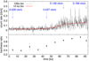 |
Fig. 1. Light curves and hardness ratio. Upper panel: pn light curve binned into 100 s bins (black solid line) with the long-term flux evolution shown as a low-resolution version of the light curve binned into 10 ks bins (red line). Arrows with labels show the corresponding count rate (in the red line) at selected points where the trend of the low resolution light curve changes. Lower panel: Hardness ratio (1.0–10.0 keV band divided by 0.2–1.0 keV band) calculated from low-resolution light curves binned into 10-ks bins. |
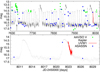 |
Fig. 2. OM light curve (red solid line) compared to AAVSO and ASAS-SN V data and Kepler magnitudes. In the upper panel, the Kepler light curve is shifted in time by +1775 days in order to superimpose the superoutburst in Kepler and AAVSO data marked by the arrow. In the lower panel, the Kepler data are shifted horizontally by +1800.8 days to compare the OM and ASAS-SN light curve with a randomly selected regular outburst. |
Finally, because of the low brightness of the object (average net pn count rate of 0.0365) the high-resolution RGS spectra are not suitable for quantitative spectral analysis – even if the object is detected. Therefore, we need to rely on the low-resolution spectra from the EPIC pn detector. We extracted the pn spectrum with evselect using the same (re-generated) calibrated pn events file used for light curve extraction. The same extraction regions as in pn light curve were used. Standardly used (recommended) quality flags were used. The rmf and arf files were generated using rmfgen and arfgen tools. The spectra were grouped using the specgroup tool and rebinned to contain 25 photons per bin. Two spectra were extracted based on the brightness evolution (see next section for more details).
3. Light-curve evolution
The mean flux and hardness ratio of the X-ray light curve are shown in Fig. 1. There is a visible change in behaviour between approximately 50 and 60 ks of elapsed observing time. To understand this phenomenon, we compared the OM light curve with data taken from the AAVSO, ASAS-SN and Kepler (the same data as in Dobrotka & Ness 2015) in Fig. 2. In order to identify the activity stage during the XMM-Newton observation, a direct comparison of Kepler and XMM-Newton light curves would be optimal. However, we have no simultaneous Kepler data and the existing Kepler light curve can be used at least for comparison of the phenomenology. Therefore, we shifted the Kepler data in time in order to ‘synchronise’ them with one randomly selected super-outburst seen in the AAVSO data (marked by the arrow in the upper panel of Fig. 2). The upper panel of Fig. 2 clearly shows that the XMM-Newton observation was not taken during optical quiescence. The lower panel of Fig. 2 compares the OM data with a randomly selected and horizontally shifted regular outburst in the Kepler data. The OM and ASAS-SN data agree well with a regular outburst behaviour. Therefore, we conclude that the XMM-Newton observation was taken during the decline from an outburst.
For further analysis, we divided all light curves into two sub-samples, an initial (first 45 ks in pn light curve) low flux and a final (after 64.98 ks in pn light curve) high-flux portion (see Fig. 1). The region in between is excluded as a transition region. These time intervals are selected based on the low resolution light curve. They represent points where the flux changed considerably in behaviour (second and third arrow in Fig. 1).
4. Spectral study
We used XSPEC1 (Arnaud 1996) to test spectral models against pn spectra via χ2 statistics. All photons below 0.3 keV and above 10 keV were ignored. This results in spectral bins up to approximately 7–8 keV. Therefore, we fixed the fitted interval to 0.3–7.0 keV. Since we are interested in the soft part, we display the spectra in Fig. 3 from 0.2 keV, as allowed by XMM-Newton thread2. The models were extrapolated to this lower energy value in order to search for any soft excess. Finally, we fit the data also from 0.2 keV, finding the results are very consistent with the 0.3 keV version described below.
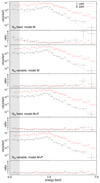 |
Fig. 3. EPIC pn spectra from different parts of the pn light curve with corresponding fits and ratios between data and fitted model. Parts 1 and 2 represent low and high flux portion of the data, respectively. Two models are shown (see text or Table 1 for details). The fits are performed from 0.3 keV and the shaded area represents an extrapolated region. |
We took photoelectric absorption within the neutral interstellar medium plus the photoelectric absorption of the circumstellar material into account using the tbabs model (Wilms et al. 2000). The only parameter of tbabs is the neutral hydrogen column density NH, while the column density of other neutral elements in the line of sight are computed assuming cosmic abundances. As an independent estimate for the amount of interstellar absorption in the direction of V1504 Cyg we use the HEASARC NH tool3. Several (but very similar) values were computed from the HI4PI survey (HI4PI Collaboration 2016) resulting in a mean value of 9.81 × 1020 cm−2.
For the spectral fitting, we used the cooling-flow model mkcflow (Mushotzky & Szymkowiak 1988) that Mukai et al. (2003) applied to CV spectra. The model is based on the radiative energy release in the form of optically thin plasma in local collisional equilibrium that cools in a steady-state flow. The observed radiation can be modeled with the isothermal APEC model (Smith et al. 2001) or a combination of them, and the XSPEC model mkcflow assumes the flow as an interpolation between a minimum (Tlow) and a maximum (Thigh) APEC X-ray temperature. The APEC model basically assumes a collisional plasma in equilibrium, thus collisional ionisation and excitations being balanced by radiative recombination and de-excitations. Such a spectrum consists of bremsstrahlung continuum and emission lines. The key parameter is the electron temperature, T, which originates from a Maxwellian velocity distribution of electrons and ions as a result of collisional equilibrium. An isothermal plasma is unlikely in nature, and it is more likely that it is a broad distribution of temperatures, while the mkcflow model is one possible realisation of a non-isothermal plasma.
The mkcflow model has originally been developed for galaxy clusters for which the redshift z is an important parameter. In addition to shifting the spectra, z is used to obtain the flux from the model via distance/z. As a consequence the computation of ṁacc from the normalisation fails for z = 0. For Galactic sources that do not require a spectral shift, we fix z at a small but non-zero value, z = 5 × 10⁻⁸ like in Dobrotka et al. (2017). This is equivalent to a Doppler shift of 0.015 km s−1, which is negligible.
Another free parameter is the abundance of elements heavier than hydrogen relative to Solar. In the absence of any hydrogen lines, absolute (i.e. relative to H) abundances can only be estimated assuming the number of free electrons forming the bremsstrahlung continuum is equivalent to the number of hydrogen ions. This is highly uncertain because the determination of the bremsstrahlung continuum assumes all additional emission lines are correctly included in the atomic database, while a large number of weak emission lines are poorly known. Given the high uncertainty, we performed the subsequent fits with abundances fixed to solar. In any case, using the abundance as a free parameter does not improve the fits.
The fitted mkcflow models are depicted in the upper two panels of Fig. 3. We used the aforementioned NH value as a fixed (top) and as a start value, while keeping it variable (second panel). The survey value comes from interpolation of several measurements, therefore, some deviation from the derived value is acceptable. Apparently, the model with fixed NH leaves a deficiency in the soft part of both spectra, which could indicate overestimated absorption or a soft excess. This is supported by the model with variable NH yielding better agreement with the soft part of the observed spectrum. A deficit of the fit in the hard band of the first part of the spectra can also be seen. Variable NH yields an improvement also in this case, but some hard excess is still possible. The fit parameters are listed in Table 1 (M model).
Summary of fitted parameters.
We tested an alternative scenario to improve the soft deficit in the model with fixed NH. Balman et al. (2014) added a powerlaw model to their spectral fits to Swift spectra of MV Lyr and interpreted it as possible scattering effects of X-rays from a wind or extended component. Resulting fits with fixed or variable NH are depicted in Fig. 3 as the M+P models (with parameters summarised in Table 1). Apparently, adding this component to the mkcflow can also remedy the soft deficit and it also improves the hard-band fit of the first part of the spectra. While this improvement is significant in the first part of the spectra where  decreased from 1.46 to 1.12, the second part did not improve. Such an improvement of the fits using an additional powerlaw component only in the first part and not in the second is supported using F-test.
All models yield upper limits of Tlow below 1 keV, and Thigh tends to be lower in the first part of the spectra. Moreover, the latter parameter reaches considerably lower values when a powerlaw model is added. The ṁacc parameter tends to be higher in the spectrum extracted from the second episode of the light curve4. Since ṁacc is the normalisation of the cooling-flow model, the rise of this parameter is a result of increasing luminosity during the second part of the light curve. The physical reason for such a luminosity increase can be higher radiation efficiency, therefore, the ṁacc values must be taken with caution.
Finally, we tried also to add a black-body component in order to investigate possible soft excess attributed to an optically thick boundary layer. We did not get any fit improvement. The resulting  remained almost the same or slightly worse, compared to models without a black body. Moreover, extrapolated models in Fig. 3 down to 0.2 keV do not show any noticeable soft excess. Therefore, we conclude that no black-body component can be identified.
5. Fast variability study
Dobrotka & Ness (2015) and Dobrotka et al. (2016) studied optical flickering of V1504 Cyg, finding a break frequency at log(f/Hz) = −3 during the outburst. They proposed that this characteristic break frequency may originate from the inner parts of the geometrically thin disc, which was truncated during quiescence. However, a very similar value was found in the optical (Scaringi et al. 2012) and X-ray (Dobrotka et al. 2017) data of MV Lyr. The presence in both bands imply that the sandwich corona can be the origin of the variability. MV Lyr shows also potential variability with higher frequency of log(f/Hz) = −2.4 found in XMM-Newton (Dobrotka et al. 2019) and NuSTAR light curves (Balman et al. 2022), although the latter display a large error interval in the range from −2.2 to −2.9. For this reason, we searched for any variability pattern in our X-ray data of V1504 Cyg.
5.1. Power density spectrum study
For the PDS study, we divided the light curve into several sub-samples. Subsequently, using the Lomb-Scargle algorithm5 (Scargle 1982) we calculated log-log periodograms for each of these subsamples. These periodograms were averaged and re-binned into equally spaced bins with a minimum number of periodogram points per bin. The averaging was performed over log(p), rather than p, following Papadakis & Lawrence (1993). Moreover, such an averaging of log(p) yields symmetric errors (see e.g. van der Klis 1989; Aranzana et al. 2018). The averaging and binning reduce the PDS noise, but affect the frequency resolution of the PDS. Therefore, an empirical compromise between noise and resolution must be found. The PDS low-frequency end is defined by the duration of each light curve sub-sample while the high-frequency end is determined by the Nyquist frequency. The resulting PDSs were rms-normalised (Miyamoto et al. 1991).
All PDSs estimated in this work were calculated using light curves with 100 s resolution splitted into three sub-samples, and re-binned using a bin width of 0.1 in log scale, and a minimum number of points per bin of 3 × 3 (i.e. three sub-samples and three points from each corresponding periodogram).
As confidence test, we used simulations following Timmer & Koenig (1995). For this purpose, the observed PDSs were fitted with a broken power-law fit. In the log-log representation, such a fit consists of a decreasing linear function with frequency describing the red noise and a constant for the highest frequencies as Poisson noise if needed. The red noise slope summarised in Table 2 is used as an input parameter for the simulations and red noise light curves with added Poisson noise were calculated. The simulated light curves have the same sampling, mean count rate, and amplitude of variability σrms (see next section) as the observed data. If a long-term trend is present (OM data), the light curve is first detrended using a polynomial. The red noise slope for the simulations is measured after the detrending and the polynomial is added to every simulated light curve. Subsequently, a PDS is calculated using the same method and parameters setup as used for the real data. We repeated the process 1000 times and the mean value of the power with σ was calculated. For the detection of significant patterns, we used at least a 2-σ level.
Red noise slopes of final PDS models: broken power law with a break frequency in the second part of the EPIC light curve and simple red noise in other sub-samples.
As input X-ray light curves, we used combined pn, MOS1, and MOS2 light curves, because using only the pn data would yield an overly low confidence for the PDS patterns. Figure 4 shows the resulting PDSs from the first and second part of the data with durations of 40 ks and 30.5 ks, respectively. All points in the first part lies within 2-σ limit of a white noise. Therefore, we conclude that PDS of the first part is flat and dominated by Poisson noise. The second part of the data already shows some trends. There is a break at log(f/Hz) = −3.02 ± 0.13. Above this frequency, the power decreases as expected from red noise, and the Poisson white noise level dominates from log(f/Hz) = −2.48 ± 0.11. Apparently, the white noise 2-σ interval is not able to reproduce the PDS. Using the red noise model instead improves the situation, but the PDS point at log(f/Hz) = −2.48 still lies below the 2-σ limit. In order to describe all PDS points, a multi-component model (depicted by the solid red line in Fig. 4) is needed. Therefore, the break at log(f/Hz) = −3.02 is real, with an approximately 2-σ confidence.
 |
Fig. 4. PDSs calculated from combined EPIC light curves from first (upper panel) and second (lower panel) part of the data. Crosses are the mean values of the PDS power at a mean frequency of every bin. The error bars represent bin widths and errors of the mean. Vertical dotted lines show the orbital frequency, forb, and its first harmonics. Blue lines represent the 2-σ confidence intervals from simulations of noises. |
Figure 5 shows PDSs calculated from first and second part of OM data with durations of 49.3 ks and 23.2 ks, respectively. These light curves show strong long-term trend which was accounted for during the simulations. The upper panel of Fig. 5 shows 2-σ intervals for the first part of the OM data. The white noise case does not describe the PDS well, while the red noise model is much better and all PDS points are within the 2-σ interval. Therefore, the red noise nature of the variability is clear. The lower panel of Fig. 5 shows PDS calculated from second part of the OM data. Investigation of the variability nature is more difficult because of short sub-sample duration. Both white and red noise cases describe all data points within 2-σ interval, but (subjectively) the red noise case is a better match. We conclude that even if the red noise nature of the variability is not conclusive, it is more likely.
5.2. Amplitude of variability
The absolute amplitude of variability is defined as square-root of the variance:
 (1)
(1)
where N is the number of the light curve points used to calculate σrms, ψi is the i-th flux point, and  is the mean value of ψi calculated from the same N points. In all subsequent analyses, we used N = 10.
Figure 6 represents the σrms time evolution of both the pn and OM light curves. Five adjacent σrms points are averaged to obtain the mean σrms. The different time evolution in both bands is obvious. The σrms in X-rays shows two different stages. This behaviour is similar to the mean flux evolution represented by the low resolution light curve in Fig. 1. Apparently, the X-ray σrms is correlated with the mean flux. The same is valid also for the UV light curve, but its time evolution is different. The σrms just decreases with the UV flux and does not show any significant deviation in behaviour related to the two-phase character seen in the X-ray data.
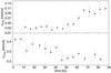 |
Fig. 6. Amplitude of variability σrms evolution with errors of the mean as uncertainty estimate for combined EPIC (upper panel) and OM (lower panel) light curves. |
6. Discussion
In this work, we studied our observation of V1504 Cyg obtained by the XMM-Newton observatory. The observation was motivated by the previous studies of V1054 Cyg optical data taken by the Kepler spacecraft (Dobrotka & Ness 2015; Dobrotka et al. 2016).
The observation was taken during the decline from an outburst and a transition phase was captured. This transition divides the light curve into two separate phases with different characteristics. For this reason, we needed to split the observation into two sub-samples. However, the transition phase is very unique and allowed us to follow the reconfiguration of the accretion disc in time.
6.1. Light curve behaviour
The X-ray light curve in Fig. 1 shows a striking change in X-ray behaviour near 60 ks after the start of the observation, that is, the overall mean flux, hardness of the radiation, and the amplitude of the variability, σrms, increased to a higher constant level by a factor of approximately 4.7, 2.5, and 2.7, respectively. While the X-ray flux rises, the UV radiation decreases (Figs. 1 and 2).
Following DIM (see Lasota 2001 for a review), which describes a DN cycle, the observed X-ray behaviour is very typical for a decline from an outburst. During this decline, a cooling front with a rarefaction wave propagates through the disc. As a consequence, the disc is depleting the accumulated matter and the surface density with overall ṁacc decreases. The disc starts to be truncated because the inner disc evaporates by coronal siphon flow due to insufficient cooling (Meyer & Meyer-Hofmeister 1994; Meyer et al. 2000) and an inner hot optically thin and geometrically thick disc forms. Such a hot disc is an ADAF (Narayan & Yi 1994, 1995; Abramowicz et al. 1995) or corona radiating in X-rays. Such ablation of the inner disc via evaporation describes well the observed delay between optical emission, UV, and X-ray in DNe (Hameury et al. 1999). As a consequence of such inner hole formation, the UV radiation generated by the receding inner disc decreases, while the X-ray radiation rises in flux because of the rebuilding of the corona. A similar X-ray brightness increase during the decline from an outburst is seen in DIM simulations (see e.g. Schreiber et al. 2003) and observations of DNe (see SS Cyg for example, Wheatley et al. 2003; McGowan et al. 2004).
What is also crucial is the different time evolution of σrms in UV and X-rays seen in Fig. 6. This divergent behaviour from the two bands suggests different physical origins of the radiation variability in the two bands. The localisation of the sources is clear, namely, the UV comes from the receding inner geometrically thin disc, while the X-ray comes from the rebuilding corona or boundary layer.
The varying X-ray and UV characteristics are already well known from some AGNs. XMM-Newton observations of IRAS 13224-3809 show that the UV variability is not correlated with X-rays (Buisson et al. 2018). Fabian et al. (2009) and Pawar et al. (2017) also showed the same for 1H 0707-495. Pawar et al. (2017) concluded that the discrepancies between the two energy bands rule out reprocessing of X-rays as the source of UV variability. AGNs are a special case, where the inner disc is truncated, resembling DNe in quiescence. The corona radiates in the X-ray and if an inner geometrically thin disc as a reprocessing region exists, the X-rays are reprocessed into optical and UV (upper illustration of Fig. 7). As a consequence these two bands should have the same characteristics such as the PDS structure or σrms evolution. This is the case of DNe in their high state, but it is better demonstrated by the high state of the nova-like variable MV Lyr (Dobrotka et al. 2017). If the inner geometrically thin disc is truncated (lower illustration of Fig. 7), a large part of the reprocessing region is missing and the detected UV radiation is not generated by reprocessing. In such a case, the UV ought to be generated by another mechanism. The intrinsic variability of the accretion flow through the remaining outer disc via propagating fluctuations is a possibility. Such variability has its ‘own’ characteristics that does not depend on the X-ray. Balman & Revnivtsev (2012) reported correlations with time lags of 96-181 s between UV and X-ray in five CVs. The authors interpret the lag as travel time of matter from a truncated inner disc to the WD surface6, therefore supporting the non-reprocessing scenario. However, some partial irradiation of the remaining disc is still possible, but the reprocessed UV power can be too weak to dominate the PDS or σrms characteristics of the light curve. Such reprocessing in quiescent DNe was shown by Balman & Revnivtsev (2012), Aranzana et al. (2018), and Nishino et al. (2022), using time lag analysis.
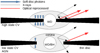 |
Fig. 7. Illustration of a possible disc configuration for DNe in different brightness states. The corona is a complex structure containing ADAF in the low state of a CV. The thin arrows show the relation between X-rays, reprocessed UV radiation and inner geometrically thin disc as reprocessing region. Much less is reprocessed into optical when the disc is truncated. Thick blue arrows show soft disc photons as source of the Compton cooling of the corona. |
6.2. Power density spectra
While we see no break frequency nor evolution in OM PDSs, the situation is different in the X-ray. The first part of the observation with lower flux is flat and does not show any characteristic frequency or red noise. The second part of the data with higher flux is characterised by a PDS showing significant red noise and a possible break at log(f/Hz) = −3.02.
This behaviour is very similar to that of SU UMa (Balman 2015). The authors interpret the break as a ‘fingerprint’ of the inner truncated disc. The radius of the truncated disc in quiescence is further away from the WD and it is closer to the WD during outburst. As a consequence, the Keplerian frequency should be lower in the former case. Moreover, if the disc almost reaches the surface of the WD, the break can disappear. The same radius versus frequency interpretation present Balman & Revnivtsev (2012) in several other DNe. Following the authors, we can see that SS Cyg in outburst does show a break in the X-ray. Moreover, Dobrotka et al. (2016) showed different behaviour for optical PDSs of V1504 Cyg and V344 Lyr. Both systems show dominant frequency close to log(f/Hz) = −3 during outburst, which disappear in quiescence. Apparently, the disappearance of break frequencies in PDSs during outburst is not always present. It is important to take into account the exact timing of the observation. If the break frequency is connected to the inner disc truncation, this truncation is evolving from outer to inner radii during the rise of the outburst and reverse back during the outburst decline. If the observation is taken during the outburst, but closer to the rising or declining part, the truncation as a break frequency could still be detected. However, Dobrotka et al. (2016) took into account this timing and used various intervals covering the outburst. All cases showed the same behaviour, that is, optical PDSs show dominant frequency close to log(f/Hz) = −3 during an outburst, which disappear in quiescence. On the other hand, our non detection of any PDS pattern during the first part of the V1504 Cyg X-ray light curve can be a simple result of an overly low count rate.
Moreover, if the dominant break frequency in PDS is a fingerprint of the inner truncated radius, this frequency should increase during the transition from quiescence to outburst and vice versa. The opposite was shown by Dobrotka et al. (2020) using Kepler data of MV Lyr. The latter is a nova-like CV system in a high state that is nonetheless experiencing transitions between low and high states. Kepler observations of this binary recorded such a transition. During the decline from the high state, during which the disc truncation radius should increase, the dominant frequency at log(f/Hz) = −3 did not decrease – on the contrary, it increased.
Even if the scenario where the dominant PDS characteristic frequency is a fingerprint of the truncation radius is appealing and similar to the case of the X-ray binaries, there is an alternative. Scaringi (2014) explained the presence of log(f/Hz) = −3 frequency in optical PDS of MV Lyr by the reprocessing of X-rays into the optical. The origin of this X-ray emission should be the geometrically thick inner corona. If the dominant PDS characteristic frequency is a fingerprint, for example, of the radial extent of such corona and not the inner standard geometrically thin disc, the shrinking of the former during transition from a high to low state can produce a characteristic (Keplerian) frequency increase, rather than decrease (see top panel of Fig. 3 in Scaringi 2014). Such a radial ‘shrinking’ of the corona was observed also in AGNs by Kara et al. (2013), based on soft time lags in IRAS 13224-3809, as well as by Wilkins et al. (2014) through modelling the relativistically broadened iron Kα fluorescence line in 1H 0707-495. The authors conclude that the X-ray source is more compact during low flux states. Moreover, both authors concluded that the spatial extent of the corona can be interpreted as an increase in the height of the corona above the disc and/or they may be some radial expansion as well (see e.g. Fig. 9 of Wilkins & Gallo 2015). However, the AGN case is much more complex. The corona may contain sandwich and lamp-post components and during the flux changes, the corona can evolve or change between these two configurations. In any case, this confirms that a sandwich corona is not stable and that radial variability is indeed possible.
The similarity between V1504 Cyg and MV Lyr is based on detection of a break frequency at log(f/Hz) = −3 both in the optical and X-ray during a high state or close to it. It would be important to see whether the break frequency at log(f/Hz) = −3 is seen during the quiescence in X-rays, because it disappears in the optical in both systems (Dobrotka & Ness 2015; Dobrotka et al. 2016, 2020). Dobrotka et al. (2020) proposed that the characteristic frequency at log(f/Hz) = −3 is common in various other systems in a high state, while it is absent in the low state. The hot X-ray corona as origin of the variability as proposed by Scaringi (2014) is one model that may possibly explain such behaviour. In such cases, the coronal flow generates ṁacc fluctuations which propagate inward. These fluctuations modulate the X-ray radiation that is reprocessed into optical by the underlying optically thick disc. If such disc is truncated, a much smaller surface is left for the reprocessing (Fig. 7). As a consequence the optical radiation does not show the same timing characteristics as X-rays, that is, the break frequency at log(f/Hz) = −3 is seen in the X-ray but not in the UV (as in our case).
However, this interpretation conflicts with the missing break frequency in the first part of the X-ray light curve of V1504 Cyg, which is closer to the outburst. There are two possibilities of how to explain it. One is the solution proposed by Balman & Revnivtsev (2012) that the break frequency is generated by the inner disc edge in a truncated disc. Such a disc reaches the WD surface during the outburst and no break is expected. However, this is in contrast to the detection of the log(f/Hz) = −3 signal in optical Kepler data during the outburst (Dobrotka & Ness 2015; Dobrotka et al. 2016). Moreover, as already mentioned, the frequency evolution during transition to the low state in MV Lyr (Dobrotka et al. 2020) does not support the inner disc edge scenario in CVs. If still true, the optical variability at log(f/Hz) = −3 in Kepler data of V1504 Cyg should be generated by the inner region of optically thick disc, and the existence of the same break frequency at log(f/Hz) = −3 in both the optical Kepler and the second part of the X-ray data is not explained. It may simply be a coincidence. The second explanation is based on the sandwich model and inspired by MV Lyr case (Scaringi 2014). On the rising or declining branch of an outburst, but still far from the maximum, the inner geometrically thick corona generates X-ray variability with a frequency of log(f/Hz) = −3. We detected this in the second part of the X-ray light curve closer to quiescence. These X-rays are not sufficiently reprocessed into optical because of inner disc truncation (Fig. 7), and the optical variability with frequency log(f/Hz) = −3 is missing. During or around the outburst maximum, the lower X-ray temperature implies less evaporation. As a consequence, the corona becomes very weak and the X-ray variability is hardly detectable – as in the first part of our X-ray light curve, closer to outburst maximum. Since the X-ray power is too weak, the reprocessing cannot explain the optical variability seen in Kepler data. As in the previous scenario, this optical variability must be generated by the inner optically thick disc. In the outburst, the gas in this disc is evaporated into the corona, but it re-condensates back (Meyer et al. 2007). If the corona generates the log(f/Hz) = −3 variability via mass accretion fluctuations, these fluctuations re-condensate and propagate in the thin disc. This can generate optical variability with the same frequency. Finally, since we did not detect the log(f/Hz) = −3 variability in the first part of our X-ray nor UV light curve, the corona is still weak and the optically thick disc is already slightly truncated. Therefore, the sandwich model is able to explain the connection of X-rays with optical and detection of the same frequency in both bands.
The re-condensation of the coronal flow can yield another consequence. After such re-condensation the accretion flow via geometrically thin disc is a mixture of the ‘original’ flow with its own fluctuations, and the re-condensed contribution. Usually an accretion flow with propagating mass accretion fluctuations shows linear rms-flux relation. Therefore a mixture of two flows with different fluctuations due to different characteristics should deform the linearity of the rms-flux relation. This was observed by Dobrotka & Ness (2015) in Kepler data of V1504 Cyg. While the quiescent light curve has the expected linearity, the outburst data show the linear relation plus another component generating offset in the flux axis. This offsetting flux contribution can be generated by the “original” flow, and the variability with linear rms-flux relation together with log(f/Hz) = −3 frequency can be the result of the re-condensation.
6.3. Spectral analysis
The spectral fitting in Sect. 4 brought on two important results that are worth discussing, namely, the Thigh and ṁacc measurements. In general, the Thigh parameter tends to be higher in the second part of the data. The final values depend on the best model. While the simpler model, M, is enough to describe the second part of the data, the first part of the observation is improved after adding a power law component to the fitted model (M+P). Taking the best fits (M+P model for the first part and M model for the second part of the data), the derived Thigh 90% confidence intervals are 0.6–1.7 and 6.1–8.7 keV, respectively.
V1504 Cyg with its best fitted value intervals is cooler closer to the outburst (first part of the data). This behaviour is expected, because typical Thigh derived from X-ray spectra of DNe in outburst should be cooler compared to quiescence (see e.g. Wheatley et al. 2003; McGowan et al. 2004; Ishida et al. 2009; Collins & Wheatley 2010; Balman 2015). This is well demonstrated by AAVSO vs. RXTE observations of the prototype DN SS Cyg (McGowan et al. 2004). The quiescent temperature of this CV is reaching 26 keV derived from simple bremsstrahlung model and it decreases to about 6 keV during optical outburst. Fitting a thermal plasma model to X-ray spectra of the same object yield temperatures of 17 and 7 keV in quiescence and outburst, respectively (Wheatley et al. 2003). Moreover, the outburst of a DN is similar to nova-like systems in the high state. Balman et al. (2014) measured the Thigh parameter in few nova-like systems using Swift observations. They derived Thigh with values greater than 20 keV. In the case of MV Lyr this was confirmed by XMM-Newton observation by Dobrotka et al. (2017). Therefore, V1504 Cyg in a high state is considerably cooler compared to nova-likes and prototypical SS Cyg in similar stage. Closer to V1504 Cyg temperatures is SU UMa case with values of 8 and 4 keV in quiescence and outburst, respectively (Collins & Wheatley 2010). Finally, V1504 Cyg during outburst resembles more the CV system WZ Sge (Balman 2015). The fitted temperature of WZ Sge increased from 1 keV during the outburst to 30 keV in quiescence. The former match well our measurement of V1504 Cyg, while the latter is considerably larger. However, our observation was taken on the way to quiescence, therefore, the ‘final’ physical conditions of the quiescent flow were not yet stabilised.
Moreover, during the outburst of WZ Sge, a power-law component in X-ray spectra is present, which disappears toward quiescence (Balman 2015). It suggests thermal Comptonization of the optically thick disc photons and/or scattering from the wind. The same result was derived by Balman et al. (2014) from X-ray spectra of BZ Cam and MV Lyr in the high state, which resembles DNe in the outburst. A power law component was needed to find an acceptable fit in these two nova-like CV systems, and is explained by the presence of a wind outflow. The presence of a power law component closer to the outburst maximum (first part of the observation) in our observation of V1504 Cyg matches the mentioned cases and suggests the presence of a wind outflow. Therefore, our study of V1504 Cyg (together with other findings) implies that wind outflows are common in the high states of CVs. Finally, thermal Comptonization of the soft disk photons can still be another or additional cause of the power law in the outburst spectra. The proposed geometry in Fig. 7 describes why such Comptonization should be stronger in a high state. The geometrically thin disc penetrates deeper underneath the central part of the corona and the irradiation by soft photons from the optically thick disc is stronger. This results in corona cooling via an inverse Compton process, and the X-ray temperature is lower. This process is known from X-ray binaries (see e.g. Done et al. 2007 for review).
The ṁacc parameter 90% confidence intervals derived from best spectral fits are (0.56 − 1.02)×10−12 M⊙ yr−1 and (1.02 − 1.45)×10−12 M⊙ yr−1 for the first and second part of the data, respectively. However, this spectrally derived parameter is dependent on red-shift, which was estimated very roughly. Another way of estimating ṁacc is to use the theoretical assumption that approximately half of the gravitational potential energy is liberated by the interaction of the matter flow and the WD; LX = GMWDṁacc/2rWD, where LX is the X-ray luminosity, G is the gravitational constant, MWD is the WD mass, and rWD is the WD radius. As input parameters, we used the V1504 Cyg Gaia distance of 553.5 pc (Bailer-Jones et al. 2021), best-fit unabsorbed luminosities from Table 1 and the rWD estimate from analytical approximation of the mass-radius relation by Nauenberg (1972). In order to get ṁacc in the ranges summarised in Table 1, we need a WD mass of 0.44–0.64 M⊙ and 1.03–1.16 M⊙ for the first and second part of the data, respectively. The resulting WD masses are realistic and the different values probably result from different radiation efficiency in the two brightness stages. Assuming a WD with a mass of 1 M⊙ and unchanged radiation efficiency, the ṁacc values are 0.23 × 10⁻¹² M⊙ yr−1 and 1.54 × 10⁻¹² M⊙ yr−1. Apparently, the unknown WD mass and rough estimate of the red-shift brings some uncertainty in the ṁacc estimate, but what is important is that the value of radiation efficiency dependent ṁacc is on the order of 10−13 and 10−12 M⊙ yr−1, as derived with the spectral modelling.
Based on the general phenomenology of DNe, the brightness decline from an outburst is generated by decreasing ṁacc. Based on DIM simulations ṁacc should decrease from, for example, 10−9 to 10−14 M⊙ yr−1 (see e.g. Fig. 3 of Hameury et al. 2000). Therefore, it seems like the rising ṁacc derived spectroscopically from our XMM-Newton observation of V1504 Cyg during the outburst decline contradicts this expectation. Nevertheless, during the decline from an outburst, the inner disc is truncated via evaporation (Meyer & Meyer-Hofmeister 1994) into radiatively inefficient ADAF (Meyer et al. 2000). As a result, the advective characteristics of the emitting plasma start to change, making the plasma more luminous. Therefore, the changing ṁacc does not necessarily describe the real ṁacc evolution.
If we still assume that the small value of ṁacc is real because only a small fraction of ṁacc is evaporated into the corona, the majority of the accreted mass should flow through the underlying geometrically thin disc, and the corresponding boundary layer should be optically thick and seen as a soft component in the X-ray spectra. We did not detect it. As mentioned in Sect. 1, only very few DNe show this optically thick boundary layer and similar searches for this soft component in nova-like systems was not successful. Apparently, the existence of an optically thick boundary layer in the high state of CVs is questionable even if the theory predicts it.
7. Summary and conclusions
We observed the DNe V1504 Cyg with XMM-Newton during the decline from an outburst covering a specific transition phase during which the X-ray flux, amplitude of the variability, and the hardness ratio have risen in a very short time interval. The UV light curve did not follow this trend, it only decreased in flux and amplitude of the variability. This different behaviour of X-ray and UV light curve we explain by a truncated inner disc and a missing reprocessing region.
A spectral fitting assuming a cooling-flow model revealed higher temperatures and mass accretion rate during the second part of the observation when the X-ray flux was higher. The first part of the data with lower X-ray flux is better described by an additional power-law component. This component should represent the scattering in an outflow, which was already observed in nova-like systems in the high state (Balman et al. 2014) or thermal Comptonization of the soft-disk photons. The rising mass transfer rate during the decline from an outburst derived with spectral modelling reflects the changing radiation efficiency of the evaporating inner disc and not the real increase of the mass flow. Such radiation inefficiency is typical for ADAFs.
A timing analysis of the observation showed a flat PDS during the low flux part of the observation, while the second part with higher flux showed a red noise shape with a potential break frequency at log(f/Hz) = −3.02, with a confidence of approximately 2-σ. This detection agrees with the break frequency detected in the optical by Dobrotka & Ness (2015) and Dobrotka et al. (2016). The authors proposed that this frequency is generated by the innermost parts of the accretion disc. The X-ray nature of the variability found in this work implies a connection with the central hot optically thin plasma. Moreover, a similar frequency was observed in several other cataclysmic variables during the high state, while it was missing during the low state. Based on the reprocessing geometry, a sandwich model where a geometrically thick ADAF-like corona surrounds the geometrically thin disc is a plausible accretion configuration.
This is not valid for the values derived from M+P model with fixed NH parameter, but based on best fits it is valid.
We used python’s package Astropy (Astropy Collaboration 2013, 2018, 2022).
We cannot confirm nor deny such correlation in V1504 Cyg, because the cross-correlation function is unclear and yields no conclusive results. Its shape is more or less flat mainly in the first low flux portion of the light curve. This is not surprising because compared to e.g. MV Lyr, where such crosscorrelation was studied (Dobrotka et al. 2017), our X-ray light curve of V1504 Cyg has a count rate that is 10 to 100 times lower.
Acknowledgments
AD was supported by the Slovak grant VEGA 1/0408/20, and by the European Regional Development Fund, project No. ITMS2014+: 313011W085. We acknowledge with thanks the variable star observations from the AAVSO International Database contributed by observers worldwide and used in this research. This work makes use of ASAS-SN (Shappee et al. 2014, Kochanek et al. 2017) and Kepler data (Borucki et al. 2010). We thank the anonymous referee for very helpful comments.
References
- Abramowicz, M. A., Chen, X., Kato, S., Lasota, J.-P., & Regev, O. 1995, ApJ, 438, L37 [NASA ADS] [CrossRef] [Google Scholar]
- Aranzana, E., Körding, E., Uttley, P., Scaringi, S., & Bloemen, S. 2018, MNRAS, 476, 2501 [Google Scholar]
- Arévalo, P., & Uttley, P. 2006, MNRAS, 367, 801 [Google Scholar]
- Arnaud, K. A. 1996, ASP Conf. Ser., 101, 17 [Google Scholar]
- Astropy Collaboration (Robitaille, T. P., et al.) 2013, A&A, 558, A33 [NASA ADS] [CrossRef] [EDP Sciences] [Google Scholar]
- Astropy Collaboration (Price-Whelan, A. M., et al.) 2018, AJ, 156, 123 [Google Scholar]
- Astropy Collaboration (Price-Whelan, A. M., et al.) 2022, ApJ, 935, 167 [NASA ADS] [CrossRef] [Google Scholar]
- Bailer-Jones, C. A. L., Rybizki, J., Fouesneau, M., Demleitner, M., & Andrae, R. 2021, AJ, 161, 147 [Google Scholar]
- Balman, Ş. 2015, Acta Polytech. CTU Proc., 2, 116 [CrossRef] [Google Scholar]
- Balman, Ş. 2020, Adv. Space Res., 66, 1097 [NASA ADS] [CrossRef] [Google Scholar]
- Balman, Ş., & Revnivtsev, M. 2012, A&A, 546, A112 [NASA ADS] [CrossRef] [EDP Sciences] [Google Scholar]
- Balman, Ş., Godon, P., & Sion, E. M. 2014, ApJ, 794, 84 [NASA ADS] [CrossRef] [Google Scholar]
- Balman, Ş., Schlegel, E. M., & Godon, P. 2022, ApJ, 932, 33 [NASA ADS] [CrossRef] [Google Scholar]
- Borucki, W. J., Koch, D., Basri, G., et al. 2010, Science, 327, 977 [Google Scholar]
- Buisson, D. J. K., Lohfink, A. M., Alston, W. N., et al. 2018, MNRAS, 475, 2306 [NASA ADS] [CrossRef] [Google Scholar]
- Byckling, K., Osborne, J. P., Wheatley, P. J., et al. 2009, MNRAS, 399, 1576 [NASA ADS] [CrossRef] [Google Scholar]
- Cannizzo, J. K., Smale, A. P., Wood, M. A., Still, M. D., & Howell, S. B. 2012, ApJ, 747, 117 [NASA ADS] [CrossRef] [Google Scholar]
- Collins, D. J., & Wheatley, P. J. 2010, MNRAS, 402, 1816 [NASA ADS] [CrossRef] [Google Scholar]
- Cowperthwaite, P. S., & Reynolds, C. S. 2014, ApJ, 791, 126 [NASA ADS] [CrossRef] [Google Scholar]
- Dobrotka, A., & Ness, J.-U. 2015, MNRAS, 451, 2851 [Google Scholar]
- Dobrotka, A., Ness, J.-U., & Bajčičáková, I. 2016, MNRAS, 460, 458 [Google Scholar]
- Dobrotka, A., Ness, J.-U., Mineshige, S., & Nucita, A. A. 2017, MNRAS, 468, 1183 [Google Scholar]
- Dobrotka, A., Negoro, H., & Mineshige, S. 2019, A&A, 631, A134 [NASA ADS] [CrossRef] [EDP Sciences] [Google Scholar]
- Dobrotka, A., Negoro, H., & Konopka, P. 2020, A&A, 641, A55 [EDP Sciences] [Google Scholar]
- Done, C., Gierliński, M., & Kubota, A. 2007, A&ARv, 15, 1 [Google Scholar]
- Fabian, A. C., Zoghbi, A., Ross, R. R., et al. 2009, Nature, 459, 540 [Google Scholar]
- Hameury, J.-M., Lasota, J.-P., & Dubus, G. 1999, MNRAS, 303, 39 [CrossRef] [Google Scholar]
- Hameury, J.-M., Lasota, J.-P., & Warner, B. 2000, A&A, 353, 244 [NASA ADS] [Google Scholar]
- HI4PI Collaboration (Ben Bekhti, N., et al.) 2016, A&A, 594, A116 [NASA ADS] [CrossRef] [EDP Sciences] [Google Scholar]
- Hogg, J. D., & Reynolds, C. S. 2016, ApJ, 826, 40 [NASA ADS] [CrossRef] [Google Scholar]
- Ingram, A., & Done, C. 2010, MNRAS, 405, 2447 [NASA ADS] [Google Scholar]
- Ingram, A., & van der Klis, M. 2013, MNRAS, 434, 1476 [NASA ADS] [CrossRef] [Google Scholar]
- Ishida, M., Okada, S., Hayashi, T., et al. 2009, PASJ, 61, S77 [NASA ADS] [CrossRef] [Google Scholar]
- Kara, E., Fabian, A. C., Cackett, E. M., Miniutti, G., & Uttley, P. 2013, MNRAS, 430, 1408 [NASA ADS] [CrossRef] [Google Scholar]
- Kato, T., Maehara, H., Miller, I., et al. 2012, PASJ, 64, 21 [NASA ADS] [Google Scholar]
- Kelly, B. C., Sobolewska, M., & Siemiginowska, A. 2011, ApJ, 730, 52 [NASA ADS] [CrossRef] [Google Scholar]
- King, A. R., Pringle, J. E., West, R. G., & Livio, M. 2004, MNRAS, 348, 111 [NASA ADS] [CrossRef] [Google Scholar]
- Kochanek, C. S., Shappee, B. J., Stanek, K. Z., et al. 2017, PASP, 129, 1045022 [CrossRef] [Google Scholar]
- Kotov, O., Churazov, E., & Gilfanov, M. 2001, MNRAS, 327, 799 [Google Scholar]
- Lasota, J.-P. 2001, New A Rv., 45, 449 [NASA ADS] [CrossRef] [Google Scholar]
- Long, K. S., Mauche, C. W., Raymond, J. C., Szkody, P., & Mattei, J. A. 1996, ApJ, 469, 841 [NASA ADS] [CrossRef] [Google Scholar]
- Lyubarskii, Y. E. 1997, MNRAS, 292, 679 [Google Scholar]
- Mauche, C. W., & Raymond, J. C. 2000, ApJ, 541, 924 [NASA ADS] [CrossRef] [Google Scholar]
- Mauche, C. W., Raymond, J. C., & Mattei, J. A. 1995, ApJ, 446, 842 [NASA ADS] [CrossRef] [Google Scholar]
- McGowan, K. E., Priedhorsky, W. C., & Trudolyubov, S. P. 2004, ApJ, 601, 1100 [NASA ADS] [CrossRef] [Google Scholar]
- Meyer, F., & Meyer-Hofmeister, E. 1994, A&A, 288, 175 [NASA ADS] [Google Scholar]
- Meyer, F., Liu, B. F., & Meyer-Hofmeister, E. 2000, A&A, 361, 175 [NASA ADS] [Google Scholar]
- Meyer, F., Liu, B. F., & Meyer-Hofmeister, E. 2007, A&A, 463, 1 [NASA ADS] [CrossRef] [EDP Sciences] [Google Scholar]
- Miyamoto, S., Kimura, K., Kitamoto, S., Dotani, T., & Ebisawa, K. 1991, ApJ, 383, 784 [NASA ADS] [CrossRef] [Google Scholar]
- Miyamoto, S., Kitamoto, S., Iga, S., Negoro, H., & Terada, K. 1992, ApJ, 391, L21 [NASA ADS] [CrossRef] [Google Scholar]
- Mukai, K., Kinkhabwala, A., Peterson, J. R., Kahn, S. M., & Paerels, F. 2003, ApJ, 586, L77 [NASA ADS] [CrossRef] [Google Scholar]
- Mushotzky, R. F., & Szymkowiak, A. E. 1988, NATO Adv. Study Inst. (ASI) Ser. C, 53, 229 [Google Scholar]
- Narayan, R., & Popham, R. 1993, Nature, 362, 820 [NASA ADS] [CrossRef] [Google Scholar]
- Narayan, R., & Yi, I. 1994, ApJ, 428, L13 [Google Scholar]
- Narayan, R., & Yi, I. 1995, ApJ, 452, 710 [NASA ADS] [CrossRef] [Google Scholar]
- Nauenberg, M. 1972, ApJ, 175, 417 [NASA ADS] [CrossRef] [Google Scholar]
- Nishino, Y., Kimura, M., Sako, S., et al. 2022, PASJ, 74, L17 [NASA ADS] [CrossRef] [Google Scholar]
- Nogami, D., & Masuda, S. 1997, Inf. Bull. Variable Stars, 4532, 1 [NASA ADS] [Google Scholar]
- Osaki, Y. 1974, PASJ, 26, 429 [NASA ADS] [Google Scholar]
- Papadakis, I. E., & Lawrence, A. 1993, MNRAS, 261, 612 [Google Scholar]
- Pawar, P. K., Dewangan, G. C., Papadakis, I. E., et al. 2017, MNRAS, 472, 2823 [Google Scholar]
- Popham, R., & Narayan, R. 1995, ApJ, 442, 337 [CrossRef] [Google Scholar]
- Pringle, J. E. 1981, ARA&A, 19, 137 [NASA ADS] [CrossRef] [Google Scholar]
- Raykov, A. A., & Yushchenko, A. V. 1988, Peremennye Zvezdy, 22, 853 [NASA ADS] [Google Scholar]
- Scargle, J. D. 1982, ApJ, 263, 835 [Google Scholar]
- Scaringi, S. 2014, MNRAS, 438, 1233 [Google Scholar]
- Scaringi, S., Körding, E., Uttley, P., et al. 2012, MNRAS, 427, 3396 [Google Scholar]
- Schreiber, M. R., Hameury, J. M., & Lasota, J. P. 2003, A&A, 410, 239 [NASA ADS] [CrossRef] [EDP Sciences] [Google Scholar]
- Shappee, B., Prieto, J., Stanek, K. Z., et al. 2014, Am. Astron. Soc. Meet. Abstr., 223, 236.03 [Google Scholar]
- Smith, R. K., Brickhouse, N. S., Liedahl, D. A., & Raymond, J. C. 2001, ApJ, 556, L91 [Google Scholar]
- Sunyaev, R., & Revnivtsev, M. 2000, A&A, 358, 617 [NASA ADS] [Google Scholar]
- Thorstensen, J. R., & Taylor, C. J. 1997, PASP, 109, 1359 [CrossRef] [Google Scholar]
- Timmer, J., & Koenig, M. 1995, A&A, 300, 707 [NASA ADS] [Google Scholar]
- Uttley, P., McHardy, I. M., & Vaughan, S. 2005, MNRAS, 359, 345 [NASA ADS] [CrossRef] [Google Scholar]
- Van de Sande, M., Scaringi, S., & Knigge, C. 2015, MNRAS, 448, 2430 [Google Scholar]
- van der Klis, M. 1989, NATO Adv. Sci. Inst. (ASI) Ser. C, 262, 27 [Google Scholar]
- Vikhlinin, A., Churazov, E., Gilfanov, M., et al. 1994, ApJ, 424, 395 [NASA ADS] [CrossRef] [Google Scholar]
- Warner, B. 1995, Cataclysmic Variable Stars Camb. Astrophys. Ser., 28 [Google Scholar]
- Wheatley, P. J., Mauche, C. W., & Mattei, J. A. 2003, MNRAS, 345, 49 [CrossRef] [Google Scholar]
- Wilkins, D. R., & Gallo, L. C. 2015, MNRAS, 449, 129 [NASA ADS] [CrossRef] [Google Scholar]
- Wilkins, D. R., Kara, E., Fabian, A. C., & Gallo, L. C. 2014, MNRAS, 443, 2746 [NASA ADS] [CrossRef] [Google Scholar]
- Wilms, J., Allen, A., & McCray, R. 2000, ApJ, 542, 914 [Google Scholar]
- Zamanov, R., Latev, G., Boeva, S., et al. 2015, MNRAS, 450, 3958 [NASA ADS] [CrossRef] [Google Scholar]
- Zdziarski, A. A. 2005, MNRAS, 360, 816 [CrossRef] [Google Scholar]
All Tables
Red noise slopes of final PDS models: broken power law with a break frequency in the second part of the EPIC light curve and simple red noise in other sub-samples.
All Figures
|
Fig. 1. Light curves and hardness ratio. Upper panel: pn light curve binned into 100 s bins (black solid line) with the long-term flux evolution shown as a low-resolution version of the light curve binned into 10 ks bins (red line). Arrows with labels show the corresponding count rate (in the red line) at selected points where the trend of the low resolution light curve changes. Lower panel: Hardness ratio (1.0–10.0 keV band divided by 0.2–1.0 keV band) calculated from low-resolution light curves binned into 10-ks bins. |
| In the text | |
|
Fig. 2. OM light curve (red solid line) compared to AAVSO and ASAS-SN V data and Kepler magnitudes. In the upper panel, the Kepler light curve is shifted in time by +1775 days in order to superimpose the superoutburst in Kepler and AAVSO data marked by the arrow. In the lower panel, the Kepler data are shifted horizontally by +1800.8 days to compare the OM and ASAS-SN light curve with a randomly selected regular outburst. |
| In the text | |
|
Fig. 3. EPIC pn spectra from different parts of the pn light curve with corresponding fits and ratios between data and fitted model. Parts 1 and 2 represent low and high flux portion of the data, respectively. Two models are shown (see text or Table 1 for details). The fits are performed from 0.3 keV and the shaded area represents an extrapolated region. |
| In the text | |
|
Fig. 4. PDSs calculated from combined EPIC light curves from first (upper panel) and second (lower panel) part of the data. Crosses are the mean values of the PDS power at a mean frequency of every bin. The error bars represent bin widths and errors of the mean. Vertical dotted lines show the orbital frequency, forb, and its first harmonics. Blue lines represent the 2-σ confidence intervals from simulations of noises. |
| In the text | |
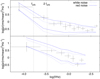 |
Fig. 5. Same as Fig. 4 but for OM data. |
| In the text | |
|
Fig. 6. Amplitude of variability σrms evolution with errors of the mean as uncertainty estimate for combined EPIC (upper panel) and OM (lower panel) light curves. |
| In the text | |
|
Fig. 7. Illustration of a possible disc configuration for DNe in different brightness states. The corona is a complex structure containing ADAF in the low state of a CV. The thin arrows show the relation between X-rays, reprocessed UV radiation and inner geometrically thin disc as reprocessing region. Much less is reprocessed into optical when the disc is truncated. Thick blue arrows show soft disc photons as source of the Compton cooling of the corona. |
| In the text | |
Current usage metrics show cumulative count of Article Views (full-text article views including HTML views, PDF and ePub downloads, according to the available data) and Abstracts Views on Vision4Press platform.
Data correspond to usage on the plateform after 2015. The current usage metrics is available 48-96 hours after online publication and is updated daily on week days.
Initial download of the metrics may take a while.