| Issue |
A&A
Volume 691, November 2024
|
|
|---|---|---|
| Article Number | L22 | |
| Number of page(s) | 10 | |
| Section | Letters to the Editor | |
| DOI | https://doi.org/10.1051/0004-6361/202451762 | |
| Published online | 26 November 2024 | |
Letter to the Editor
North Polar Spur: Gaseous plume(s) from star-forming regions ∼3–5 kpc from the Galactic Center?
1
Max Planck Institute for Astrophysics, Karl-Schwarzschild-Str. 1, D-85741 Garching, Germany
2
Space Research Institute (IKI), Profsoyuznaya 84/32, Moscow 117997, Russia
3
Universitäts-Sternwarte, Fakultät für Physik, Ludwig-Maximilians-Universität München, Scheinerstr. 1, 81679 München, Germany
4
Ioffe Institute, Politekhnicheskaya St. 26, Saint Petersburg 194021, Russia
5
Institute of Astronomy, Russian Academy of Sciences, 48 Pyatnitskaya Str., Moscow 119017, Russia
6
NRC ‘Kurchatov Institute’, Acad. Kurchatov Square 1, Moscow 123182, Russia
7
Institute of Applied Physics of the Russian Academy of Sciences, 46 Ul’yanov Str., Nizhny Novgorod 603950, Russia
⋆ Corresponding author; This email address is being protected from spambots. You need JavaScript enabled to view it.
Received:
1
August
2024
Accepted:
31
October
2024
Abstract
We argue that the North Polar Spur (NPS) and many less prominent structures are formed by gaseous metal-rich plumes associated with star-forming regions (SFRs). The SFRs located at the tangent to the 3−5 kpc rings might be particularly relevant to the NPS. A multi-temperature mixture of gaseous components and cosmic rays rises above the Galactic disk under the action of their initial momentum and buoyancy. Eventually, the plume velocity becomes equal to that of the ambient gas, which rotates with different angular speeds than the stars in the disk. As a result, the plumes acquire characteristic bent shapes. An ad hoc model of plumes’ trajectories shows an interesting resemblance to the morphology of structures seen in the radio continuum and X-rays.
Key words: Galaxy: general / X-rays: diffuse background / X-rays: galaxies
© The Authors 2024
 Open Access article, published by EDP Sciences, under the terms of the Creative Commons Attribution License (https://creativecommons.org/licenses/by/4.0), which permits unrestricted use, distribution, and reproduction in any medium, provided the original work is properly cited.
This article is published in open access under the Subscribe to Open model.
Open access funding provided by Max Planck Society.
1. Introduction
The North Polar Spur (NPS; Tunmer 1958) is a bright structure that was first discovered in all-sky radio images along with other similar structures dubbed loops (see, e.g., Dickinson 2018). Unlike other loops, the entirety of the NPS (the northern part of Loop I) is visible in soft X-rays (Bunner et al. 1972; Egger & Aschenbach 1995; Kataoka et al. 2018, 2021; Predehl et al. 2020; LaRocca et al. 2020).
Given the NPS’s large angular size, ≳90 deg, the first proposed explanation (e.g., Hanbury Brown et al. 1960; Berkhuijsen 1971) was that it was a shell of a very nearby, d ≲ 100 pc, supernova remnant (SNR). A scenario in which the NPS was a distant, d ≳ 10 kpc, Galaxy-scale structure powered by an energetic outburst in the Galactic Center (GC) region – potentially caused by an intense star formation episode in the vicinity of the GC or by the activity of the supermassive black hole Sgr A* (e.g., Sofue 1977, 1994; Sarkar et al. 2015; Sofue & Kataoka 2021; Yang et al. 2022) – was also put forward (Sofue 1977, 1994). Both scenarios suggest that the NPS is powered by a shock wave propagating in the hot medium (either interstellar or circumgalactic). This shock is responsible for the acceleration of radio-emitting relativistic electrons as well as the heating and compression of the X-ray-emitting hot gas.
Although these two scenarios involve different physical sizes, timescales, and required energetics, it has been difficult to unequivocally determine which is more likely based on the available data. Contradicting conclusions have been drawn based on, for example, Faraday rotation and X-ray absorption measurements (see a comprehensive discussion in Lallement 2023). Based on recent discoveries of the giant structures in gamma rays (Fermi bubbles; Su et al. 2010) and soft X-rays in the southern Galactic sky (eROSITA; Predehl et al. 2020), the “bubbles” appear to be more symmetric with respect to the GC, strengthening the case for the central energy release as a viable solution (e.g., Sarkar 2024).
In this Letter, we consider another scenario for NPS formation motivated by the morphological and spectral properties of the soft X-ray emission measured by eROSITA telescope in the course of the Spectrum–Roentgen–Gamma (SRG) observatory all-sky survey (Predehl et al. 2021; Sunyaev et al. 2021). We propose that the NPS was produced by a break-out of the massive star-forming regions (SFRs) associated with the end of the Galactic bar, the base of which is d ∼ 5 kpc from us (e.g., Bland-Hawthorn & Gerhard 2016). Qualitatively similar arguments have recently been discussed in Shimoda & Asano (2024). Flows of enriched hot gas move upward from the Galactic disk and get entrained in the relative rotation of the circumgalactic medium (CGM) above the disk, resulting in a spiral-like structure that appears as a loop in the sky. In this model, the advection of the enriched gas and relativistic particles, rather than a shock, is responsible for the appearance of the NPS. The model predicts a high metal abundance of X-ray-emitting gas and a lack of evolutionary signatures in the direction perpendicular to the NPS edge.
2. X-ray picture
For X-ray analysis, we used the eROSITA data from its all-sky survey. Details on the data preparation and analysis are given in Appendix A. Images extracted from the survey in the 0.52−0.61 keV and 0.7−0.96 keV bands are shown in Fig. 1 (left and middle panels, respectively). The former band includes the triplet of He-like oxygen O VII near 574 eV, while the bright lines of helium-like neon Ne IX (at 905 and 921 eV) and neon-like iron Fe XVII (between 725 and 826 eV) fall into the latter. For plasma in collisional ionization equilibrium (CIE), the peak line emissivities in these bands are at temperatures of ∼0.2 keV and ∼0.6 keV, respectively.
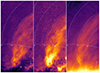 |
Fig. 1. X-ray and radio images of the NPS region. Left and middle panels: 0.52−0.61 keV and 0.7−0.96 keV eROSITA X-ray images, respectively. For comparison, the right panel shows the 408 MHz radio image from the all-sky continuum surveys (Haslam et al. 1981; Remazeilles et al. 2015). The images in galactic coordinates are shown in stereographic projection for a better view of the regions near the Galactic plane and the Galactic north pole. The X-ray images are particle-background-subtracted and exposure-corrected. The brightest compact sources and galaxy clusters have been masked, and the resulting image convolved with σ = 20′ Gaussian. Still prominently visible in the image are RS Oph (bright dot near the bottom of the left image) and the stray light halo around Sco X-1 (at the right edge of the middle image). The dashed white lines show the wedge used to extract radial profiles. The numbers indicate the distance (in degrees) from the wedge center, which is at (l, b) = (338 ° ,32 ° ) in Galactic coordinates. |
The complex X-ray morphology of the NPS is obvious from these images and their comparison. One can readily see that the correlation length of X-ray structures is larger in the direction along the NPS for both bands, but a simple combination of concentric spherical shells is not a good description of the NPS. For example, the surface brightness in the 0.52−0.61 keV band, which is dominated by the O VII line, has a sharp outer edge but a rather flat surface brightness across the inner region, unlike an edge-brightened shell. Similarly, the 0.7−0.96 keV surface brightness is composed of a fainter diffuse emission surrounding a bright central “filament”.
More quantitatively, this is illustrated via profiles of the X-ray emission in several narrow bands. Figure 1 shows a wedge that is aligned with the NPS “outer” boundary. Radial profiles extracted from this wedge are shown in Fig. 2. The steep rise, corresponding to the “edge” of NPS, is visible in all bands. However, further inside the NPS, the profiles do not follow the typical edge-brightened behavior characteristic of a spherical shock associated with an instantaneous point-like energy release in a uniform medium (see, e.g., profiles at energies below 0.61 keV). The observed profiles could be affected by the upstream gas density gradients, by non-equilibrium ionization (NEI) effects downstream of the shock, and, especially, by the energy release mode. For example, in a “steady wind” scenario (see, e.g., Sarkar et al. 2015), the surface brightness profile is rather flat. In the model without the shock that we are studying here, this behavior suggests that the volume occupied by the plasma emitting at these energies resembles a flattened sheet rather than a spherical shell. In harder bands, the profiles feature a steep jump, followed by a gradual increase in intensity before reaching a peak at x ≈ 35°. The center of the wedge is at (l, b) = (338 ° ,32 ° ) in Galactic coordinates.
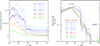 |
Fig. 2. Radial profiles of the NPS X-ray emission. Left: Observed surface brightness in several energy bands. The wedge used for the flux extraction is shown in Fig. 1. The bright edge of the NPS is at x ≈ 48°. The contributions of the instrumental background and distant (unresolved) sources composing cosmic X-ray background (CXB) have been subtracted, leaving only the flux from the Galaxy. Right: Same as the left plot, but after subtracting the mean level at x = 60 − 70°, re-normalizing by the flux at x = 35°, and lightly smoothing with a Gaussian filter (σ = 0.4°). In addition, the radio surface brightness profile (Haslam, 408 MHz) after applying the same procedure (subtraction, re-normalization, and smoothing) is shown with the dashed red curve. |
An alternative to the local SNR- or GC-related scenarios, which associate the steep rise with a shock, is the assumption that the NPS is a multi-temperature gas, where a hotter component (> 0.3 keV), responsible for the emission in iron lines above 0.7 keV, coexists with a warm plasma (e.g., 0.15−0.2 keV), which produces the bulk of the emission below 0.7 keV and most prominently in the oxygen lines. The sharpness of the NPS edge is a strong argument in favor of the shock scenario (e.g., Predehl et al. 2020). However, there are examples of astrophysical objects for which very sharp edges are seen in the hot X-ray-emitting plasma. The most relevant are “cold fronts” in galaxy clusters (see Markevitch & Vikhlinin 2007; Zuhone & Roediger 2016, for reviews). These cold fronts are contact discontinuities rather than shocks, and they might retain their sharpness due to magnetic fields and/or accelerated gas motions along the front (see, e.g., Churazov & Inogamov 2004). Similar effects might be relevant to the rising plumes discussed here.
Accurate temperature and abundance measurements for gas with temperatures below 1 keV (at which pure bremsstrahlung continuum is very weak and subdominant to other continuum components) are highly model-dependent. As is clear from Fig. 2, the ratio of fluxes in different bands varies strongly across the NPS. This means that the best-fitting temperature strongly depends on the region used for spectrum extraction. It further implies that a mixture of components with different temperatures (and different ionization states, especially in the shock-based scenario) will inevitably be present. The abundance determination for the gas in the relevant temperature range (0.1−0.6 keV) is highly degenerate with the emission measure even when the gas is in CIE. In practice, it is difficult to measure the abundance if it is larger than ∼0.1 solar. The effects of NEI, which is expected in the shock scenario, further affect the “apparent” temperature and abundance. These issues are likely the reason for the different temperature and abundance measurements in the literature (e.g., Kataoka et al. 2013; Yamamoto et al. 2022) for various patches of the NPS. The exceptionally uniform and sensitive eROSITA all-sky data give a clear view of the amplitude of spectral variations across such large regions for the first time. We defer an extended spectral analysis of the NPS to future work.
3. Morphological model
We considered a simple morphological model that is based on a broad-brush picture of the evolution of a massive SFR in the Galactic disk (e.g., Norman & Ikeuchi 1989; Kim et al. 2020). The first shock waves of supernova explosions originating from the most massive newborn stars in such a region produce hot and dense gas strongly enriched with metals of the ejecta. Initially confined by the surrounding dense and cold gas, the hot gas manages to break through and form an (adiabatically cooled) plume that moves away from the disk and interacts with the interstellar medium (ISM) and CGM, forming chimneys and plumes (see Appendix E). The trajectories of rising plumes might be complicated, especially when the gas is multiphase and magnetized. They are also affected by the pressure, magnetic fields, and velocities in the ambient ISM and/or CGM (e.g., Faucher-Giguère & Oh 2023).
For illustration purposes, we considered an ad hoc model that encapsulates all the complicated physics in three parameters: the initial (vertical) velocity of the plume (vz, 0) and two effective scale heights (zϕ and zz). The zϕ describes how the plume that initially moves together with stars and gas close to the disk plane decelerates and joins the pressure-supported hot halo gas, which is either nonrotating or rotating more slowly than the stellar disk. The zz parameter controls the decline of the vertical (perpendicular to the disk) velocity component. As a result, the two velocity components have the following dependence on z:
![Mathematical equation: $$ \begin{aligned} v_z(z) = v_{z,0} \, e^{-z/z_z} \;\;\mathrm{and}\;\; v_{\phi }(z) = v_{\rm rot} \, \left[1- e^{-z/z_\phi }\right]. \end{aligned} $$](/articles/aa/full_html/2024/11/aa51762-24/aa51762-24-eq1.gif) (1)
(1)
A flat rotation curve with vrot = 220 km s−1 was adopted for the sake of simplicity, the effective scale heights were set to zϕ = 2 kpc and zz = 5 kpc, and vz, 0 = 200 km s−1. The choice of these parameters is rather arbitrary, but it suffices for illustration purposes and the results are not dramatically sensitive to it. For the source of the plume, for example a SFR, we assumed a circular trajectory in the disk plane with the velocity vϕ,src. In our illustrative model, the following two versions were considered:
 (2)
(2)
where R is the distance from the GC. Version (a) corresponds to the source moving with the same velocity as stars, while version (b) mimics a pattern motion. The former case is relevant when the active phase of a given SFR associated with the dense gas is very long and the active region always moves together with the gas (with the velocity vrot). The latter case corresponds to a situation when the spatial distribution of the plume sources is linked to the Galactic bar and/or spiral arms. To illustrate this case, we adopted the value Ω = 33 km s−1 kpc−1 derived for the bar pattern speed (e.g., Clarke & Gerhard 2022). As a further simplification, we assumed that none of these parameters depend on the position of the plume within the galaxy.
The above relations (1) and (2) can be trivially integrated to derive a position of the gas lump released some time ago, t, relative to the current position of the “source”. By design, plume trajectories appear in 3D as spirals rising from the disk from the current location of the plume source (see Appendix B and Fig. B.1). We note here that for a very under-dense lump, the buoyancy force is solely set by pressure gradients in the ambient gas. These gradients themselves depend on the rotation velocity of the halo gas and can have both radial and vertical components. In our model, we explicitly neglected the former component, although in real systems it can force the plume to move radially. In particular, for a slow (fast) rotation of the halo gas, under-dense lumps can move to larger (smaller) radii (see Fig. B.2).
As a final step, we projected the trajectory onto the sky as seen from the position of the Sun. This modifies the appearance of the plume due to different distances from the Sun to various segments of the plume and the Sun’s motion relative to the source. An example of plume trajectories for a set of “sources” chosen by hand is shown in Fig. C.1. A table with the positions of sources is given in Appendix B. The trajectories were integrated for ∼140 Myr, which is approximately one rotation period around the GC near the Sun for the adopted value of vrot.
Figure C.1 illustrates the key morphological properties of the plumes. Naturally, the trajectories remain confined to the regions defined by the radial distance to the source from the GC, while the notable left–right asymmetry is imposed by the rotation direction of the Galaxy. All trajectories have rising parts close to the Galactic plane, with the direction of the curvature set by the mutual position of the source and the Sun and the direction of the Galaxy rotation. This is clearly illustrated by the family of trajectories for sources located at the 5 kpc ring around the GC. The morphological difference is even more pronounced for sources located at greater distances from the GC (cases marked as Cygnus X and Vela in Table B.1). For the Cygnus X region, the plume’s apparent trajectory rises to the Galactic poles before forming a spiral. For the Vela region, the plume is bent much earlier and follows an almost horizontal line at |b|∼20 − 25°.
If the NPS is indeed a gaseous plume, its base should be associated with the SFRs that are currently at Galactic longitudes l ∼ 20 ° −40° (see Fig. C.1). Incidentally, this range of longitudes corresponds to the tangential direction to the 3−5 kpc rings around the GC and hosts the most active SFRs in the Galaxy, including the prototypical mini-starburst complex W43 (see Appendix F). Below we discuss this scenario in more detail.
4. Discussion
Motivated by the morphological model presented above, we assumed that the leading edge of the NPS is located at a tangent to the 5 kpc ring. In this case, the distance of the NPS base from the Sun is DSun, NPS ≈ 6.6 kpc. Of course, some parts of the plumes can be closer to the Sun, and some farther away.
Given the apparent size of the NPS on the sky, one can assume that its physical size (the “depth” along the line of sight) is on the same order as its distance from the Sun (i.e., l ∼ DSun, NPS). Based on that, we can estimate the hot gas density from the observed peak surface brightness, IX, in the 0.7−1.05 keV band. This yields a proton number density  cm−3, where Z is the metal abundance with respect to the solar value (the abundances relative to hydrogen from Asplund et al. 2009 are used here). In this derivation, we assumed that the gas is in CIE with a temperature of 0.6 keV and used the APEC model (Foster et al. 2012) to predict the emissivity. The metallicity dependence in the above expression is valid for Z/Z⊙ ≳ 0.1. The corresponding cooling time of the gas with temperature kT ≈ 0.6 keV can be estimated using the cooling function of Sutherland & Dopita (1993):
  yr.
yr.
While the 3D geometry of the NPS is uncertain, we assumed that its volume is ≈l3 (i.e., its line-of-sight extension is comparable to its transverse size) to get an estimate of the total energy (enthalpy):  erg for l = 6 kpc. Assuming that the integrated energy release associated with the formation of 1 solar mass of stars is ∼1049 erg, it needs ∼2 × 10⁶ M⊙ of gas to be converted into stars. Assuming a star formation rate of 0.1 M⊙ yr−1, it takes ∼20 Myr to generate enough energy to power the entire NPS. The long cooling time and preferential accumulation of trajectories in the NPS region imply that it could be a result of cumulative contributions from many sources.
In the simplest version of this scenario, the gas in the NPS is in pressure equilibrium with the ambient medium. If the temperature of the ambient medium is ∼0.15 keV, the regions filled with ∼0.6 keV plasma should have a ∼4 times lower density. Yet, the NPS appears much brighter than the diffuse emission of the Galaxy. There are two plausible reasons for that. One is that for lines of Fe XVII, Ne IX, and Ne X, the gas in the halo is simply too cool to produce a bright emission. The second reason is that the plumes are plausibly much more metal-rich than the halo gas. This is particularly important for O VII lines, which are present in the spectrum of the halo. The gas in the plumes could be a factor of 10 (or more) metal-richer, and even in the absence of shock it can shine prominently (see Fig. A.1). In Appendix D we argue that the plume metallicity is not much higher than the solar one.
An important implication of the model is the global asymmetry of the Milky Way’s diffuse X-ray and radio emission. The asymmetry is present even if the distribution of the plumes’ sources is itself symmetric. In 3D, the plumes can form a symmetric pattern, but the direction of the Galaxy rotation produces the apparent asymmetry when viewed from the Sun’s position. Some extra asymmetry could come from global gas motions in the Galactic halo (e.g., Mou et al. 2023), for example caused by an interaction with the satellite galaxies, but it comes on top of the “natural” east–west asymmetry. The north–south asymmetry, which is clearly visible in both the radio and X-ray sky, in this model is attributed to the asymmetry of the primary sources of the plume. When the hot gas finds its way through the dense cold gas in the disk, it may preferentially go to one side rather than forming a symmetric structure on both sides.
This model treats trajectories of individual gas plumes as independent, neglecting the hydrodynamic nature of the flows and, in particular, possible gas mixing instabilities that would naturally arise in such a situation. The sharpness of the NPS’s outer edge as well as its overall filamentary appearance might be a manifestation of the suppression of these instabilities by the well-ordered and sufficiently strong magnetic field.
The synchrotron radio emission from the NPS region is known to be polarized (see, e.g., Sun et al. 2015, for a recent analysis). The polarization implies that the magnetic field is ordered. In the model discussed above, these structures can be especially prominent plumes located at different distances from the GC. The ordering is caused by stretching the field lines during certain phases of plume evolution and/or by the halo gas motions rather than by shocks (as illustrated in Appendix E).
On a more speculative note, we remark that in this model the gas vented from the disk tends to accumulate high above the plane in the general direction of the GC. A question thus arises as to whether structures such as the eROSITA bubbles (Predehl et al. 2020) could be produced by the same mechanism. In this case, these structures can evolve on a longer timescale than implied by the shock-driven scenario. In fact, different regions across the NPS could come from gas lumps having different ages (and different SFRs) and, therefore, can have different properties.
In the proposed scenario, the NPS might be a Galactic analog of the magnetic structures directly observed to reach significant distances above the disks in many nearby galaxies, for example NGC 4217 (Stein et al. 2020). On the other hand, the NPS might also be a case similar to the off-disk parts of the so-called anomalous spiral arms in NGC 4258, which are believed to be powered by the interaction of the relativistic jet with the galactic disk (see Zeng et al. 2023, and references therein). In all these cases, we might witness signatures of the disk-halo interaction via intense feedback episodes resulting in complex multiphase and magnetized interface region (see, e.g., the review by Beck 2015).
One observational test that can rule out the plume scenario is measuring the NEI signatures in the gas, which are pertinent to the shock scenario (e.g., Yamamoto et al. 2022). For a gas electron density of ∼10−3 cm−3 and a downstream plasma velocity of ∼200 km s−1, the ionization parameter τ = ne × t ∼ 1.5 × 1011 cm−3 s is expected at a distance of 1 kpc downstream of the shock. Such scales are easily resolved for any distance to the NPS (for the “nearby” shock scenario, the ionization parameter is even lower at the same angular distance from the shock) and can be derived from the spectra. The complication here is that the NPS does not have a simple “layered” structure that allows for a clean separation of shells at different 3D distances from the edge. As a result, the lines of O VII, O VIII, Fe XVII, Ne IX, and Ne X are always present in a proportion that is difficult to predict unless the geometry of the gas distribution is specified. We discuss the NEI scenario in a forthcoming publication. There we adopt the shock-driven scenario for the NPS, consider the implications for the X-ray spectra, and compare the two scenarios.
If our model is correct, the NPS and similar structures offer a possibility to probe the rotation pattern of the hot gas in the Milky Way. Future large-grasp microcalorimetric missions capable of mapping the entire NPS region in all-sky surveys (Khabibullin et al. 2023a), such as the Line Emission Mapper (LEM; Kraft et al. 2022), will be instrumental in measuring abundances and velocities using emission lines of elements from carbon to iron across the 0.2−2 keV energy band to narrow the range of plausible models.
5. Conclusions
While the NPS is usually attributed to a shock front associated with the activity of our GC or a local SNR, we discuss an alternative scenario. We posit that metal-enriched plumes rise above the disk from active SFRs. Interactions with the hot halo gas give these plumes the appearance of bent spirals. Their shapes sensitively depend on the rotation pattern of the hot gas above the disk. These plumes are mostly hotter than the ambient gas and can be more metal-rich than the hot gas in the Milky Way halo. In this model, the NPS itself is associated with the star formation within 3−5 kpc of the GC. Fainter plumes might be associated with other SFRs in the Galaxy.
Acknowledgments
This work is partly based on observations with the eROSITA telescope onboard SRG space observatory. The SRG observatory was built by Roskosmos in the interests of the Russian Academy of Sciences represented by its Space Research Institute (IKI) in the framework of the Russian Federal Space Program, with the participation of the Deutsches Zentrum für Luft- und Raumfahrt (DLR). The eROSITA X-ray telescope was built by a consortium of German Institutes led by MPE, and supported by DLR. The SRG spacecraft was designed, built, launched, and operated by the Lavochkin Association and its subcontractors. The science data are downlinked via the Deep Space Network Antennae in Bear Lakes, Ussurijsk, and Baikonur, funded by Roskosmos. The development and construction of the eROSITA X-ray instrument was led by MPE, with contributions from the Dr. Karl Remeis Observatory Bamberg & ECAP (FAU Erlangen-Nuernberg), the University of Hamburg Observatory, the Leibniz Institute for Astrophysics Potsdam (AIP), and the Institute for Astronomy and Astrophysics of the University of Tübingen, with the support of DLR and the Max Planck Society. The Argelander Institute for Astronomy of the University of Bonn and the Ludwig Maximilians Universität Munich also participated in the science preparation for eROSITA. The eROSITA data were processed using the eSASS/NRTA software system developed by the German eROSITA consortium and analyzed using proprietary data reduction software developed by the Russian eROSITA Consortium. IK acknowledges support by the COMPLEX project from the European Research Council (ERC) under the European Union’s Horizon 2020 research and innovation program grant agreement ERC-2019-AdG 882679.
References
- Asplund, M., Grevesse, N., Sauval, A. J., & Scott, P. 2009, ARA&A, 47, 481 [NASA ADS] [CrossRef] [Google Scholar]
- Barros, D. A., Lépine, J. R. D., & Dias, W. S. 2016, A&A, 593, A108 [NASA ADS] [CrossRef] [EDP Sciences] [Google Scholar]
- Baumgartner, V., & Breitschwerdt, D. 2013, A&A, 557, A140 [NASA ADS] [CrossRef] [EDP Sciences] [Google Scholar]
- Beck, R. 2015, A&ARv, 24, 4 [Google Scholar]
- Berkhuijsen, E. M. 1971, A&A, 14, 359 [NASA ADS] [Google Scholar]
- Bland-Hawthorn, J., & Gerhard, O. 2016, ARA&A, 54, 529 [Google Scholar]
- Bunner, A. N., Coleman, P. L., Kraushaar, W. L., & McCammon, D. 1972, ApJ, 172, L67 [NASA ADS] [CrossRef] [Google Scholar]
- Bykov, A. M. 2014, A&ARv, 22, 77 [NASA ADS] [CrossRef] [Google Scholar]
- Churazov, E., & Inogamov, N. 2004, MNRAS, 350, L52 [NASA ADS] [CrossRef] [Google Scholar]
- Churazov, E., Forman, W., Jones, C., & Böhringer, H. 2000, A&A, 356, 788 [NASA ADS] [Google Scholar]
- Churazov, E. M., Khabibullin, I. I., Bykov, A. M., et al. 2021, MNRAS, 507, 971 [NASA ADS] [CrossRef] [Google Scholar]
- Clarke, J. P., & Gerhard, O. 2022, MNRAS, 512, 2171 [NASA ADS] [CrossRef] [Google Scholar]
- de Avillez, M. A. 2000, MNRAS, 315, 479 [NASA ADS] [CrossRef] [Google Scholar]
- De Buizer, J. M., Lim, W., Karnath, N., & Radomski, J. T. 2024, ApJ, 963, 55 [NASA ADS] [CrossRef] [Google Scholar]
- Dickinson, C. 2018, Galaxies, 6, 56 [NASA ADS] [CrossRef] [Google Scholar]
- Drew, J. E., Monguió, M., & Wright, N. J. 2019, MNRAS, 486, 1034 [NASA ADS] [CrossRef] [Google Scholar]
- Egger, R. J., & Aschenbach, B. 1995, A&A, 294, L25 [NASA ADS] [Google Scholar]
- Faucher-Giguère, C.-A., & Oh, S. P. 2023, ARA&A, 61, 131 [CrossRef] [Google Scholar]
- Foster, A. R., Ji, L., Smith, R. K., & Brickhouse, N. S. 2012, ApJ, 756, 128 [Google Scholar]
- Fukui, Y., Ohama, A., Hanaoka, N., et al. 2014, ApJ, 780, 36 [Google Scholar]
- Fukui, Y., Inoue, T., Hayakawa, T., & Torii, K. 2021, PASJ, 73, S405 [Google Scholar]
- Gull, S. F., & Northover, K. J. E. 1973, Nature, 244, 80 [NASA ADS] [CrossRef] [Google Scholar]
- H.E.S.S. Collaboration (Abdalla, H., et al.) 2018, A&A, 612, A1 [NASA ADS] [CrossRef] [EDP Sciences] [Google Scholar]
- Hanbury Brown, R., Davies, R. D., & Hazard, C. 1960, The Observatory, 80, 191 [NASA ADS] [Google Scholar]
- Haslam, C. G. T., Klein, U., Salter, C. J., et al. 1981, A&A, 100, 209 [NASA ADS] [Google Scholar]
- Heiles, C. 1990, ApJ, 354, 483 [NASA ADS] [CrossRef] [Google Scholar]
- Hodges-Kluck, E. J., Miller, M. J., & Bregman, J. N. 2016, ApJ, 822, 21 [NASA ADS] [CrossRef] [Google Scholar]
- Kataoka, J., Tahara, M., Totani, T., et al. 2013, ApJ, 779, 57 [NASA ADS] [CrossRef] [Google Scholar]
- Kataoka, J., Sofue, Y., Inoue, Y., et al. 2018, Galaxies, 6, 27 [Google Scholar]
- Kataoka, J., Yamamoto, M., Nakamura, Y., et al. 2021, ApJ, 908, 14 [NASA ADS] [CrossRef] [Google Scholar]
- Khabibullin, I., Churazov, E., & Sunyaev, R. 2022, MNRAS, 509, 6068 [Google Scholar]
- Khabibullin, I., Galeazzi, M., Bogdan, A., et al. 2023a, ArXiv e-prints [arXiv:2310.16038] [Google Scholar]
- Khabibullin, I. I., Churazov, E. M., Bykov, A. M., Chugai, N. N., & Sunyaev, R. A. 2023b, MNRAS, 521, 5536 [NASA ADS] [CrossRef] [Google Scholar]
- Khabibullin, I. I., Churazov, E. M., Chugai, N. N., et al. 2024, A&A, 689, A278 [NASA ADS] [CrossRef] [EDP Sciences] [Google Scholar]
- Kim, C.-G., Ostriker, E. C., Somerville, R. S., et al. 2020, ApJ, 900, 61 [Google Scholar]
- Kobayashi, C., Umeda, H., Nomoto, K., Tominaga, N., & Ohkubo, T. 2006, ApJ, 653, 1145 [NASA ADS] [CrossRef] [Google Scholar]
- Kobayashi, C., Karakas, A. I., & Lugaro, M. 2020, ApJ, 900, 179 [Google Scholar]
- Kraft, R., Markevitch, M., Kilbourne, C., et al. 2022, ArXiv e-prints [arXiv:2211.09827] [Google Scholar]
- Lallement, R. 2023, C. R. Phys., 23, 1 [NASA ADS] [CrossRef] [Google Scholar]
- LaRocca, D. M., Kaaret, P., Kuntz, K. D., et al. 2020, ApJ, 904, 54 [NASA ADS] [CrossRef] [Google Scholar]
- Li, J. J., Immer, K., Reid, M. J., et al. 2022, ApJS, 262, 42 [NASA ADS] [CrossRef] [Google Scholar]
- Mac Low, M.-M., & McCray, R. 1988, ApJ, 324, 776 [NASA ADS] [CrossRef] [Google Scholar]
- Markevitch, M., & Vikhlinin, A. 2007, Phys. Rep., 443, 1 [Google Scholar]
- Motte, F., Nony, T., Louvet, F., et al. 2018, Nat. Astron., 2, 478 [Google Scholar]
- Mou, G., Sun, D., Fang, T., et al. 2023, Nat. Commun., 14, 781 [NASA ADS] [CrossRef] [Google Scholar]
- Nguyen Luong, Q., Motte, F., Schuller, F., et al. 2011, A&A, 529, A41 [NASA ADS] [CrossRef] [EDP Sciences] [Google Scholar]
- Norman, C. A., & Ikeuchi, S. 1989, ApJ, 345, 372 [Google Scholar]
- Planck Collaboration IV. 2020, A&A, 641, A4 [NASA ADS] [CrossRef] [EDP Sciences] [Google Scholar]
- Predehl, P., Sunyaev, R. A., Becker, W., et al. 2020, Nature, 588, 227 [CrossRef] [Google Scholar]
- Predehl, P., Andritschke, R., Arefiev, V., et al. 2021, A&A, 647, A1 [EDP Sciences] [Google Scholar]
- Remazeilles, M., Dickinson, C., Banday, A. J., Bigot-Sazy, M. A., & Ghosh, T. 2015, MNRAS, 451, 4311 [NASA ADS] [CrossRef] [Google Scholar]
- Sarkar, K. C. 2024, A&ARv, 32, 1 [NASA ADS] [CrossRef] [Google Scholar]
- Sarkar, K. C., Nath, B. B., & Sharma, P. 2015, MNRAS, 453, 3827 [Google Scholar]
- Schulreich, M. M., & Breitschwerdt, D. 2022, MNRAS, 509, 716 [Google Scholar]
- Shimoda, J., & Asano, K. 2024, ApJ, 973, 78 [NASA ADS] [CrossRef] [Google Scholar]
- Sofue, Y. 1977, A&A, 60, 327 [NASA ADS] [Google Scholar]
- Sofue, Y. 1994, ApJ, 431, L91 [NASA ADS] [CrossRef] [Google Scholar]
- Sofue, Y., & Kataoka, J. 2021, MNRAS, 506, 2170 [NASA ADS] [CrossRef] [Google Scholar]
- Stein, Y., Dettmar, R. J., Beck, R., et al. 2020, A&A, 639, A111 [NASA ADS] [CrossRef] [EDP Sciences] [Google Scholar]
- Su, M., Slatyer, T. R., & Finkbeiner, D. P. 2010, ApJ, 724, 1044 [Google Scholar]
- Sun, X. H., Landecker, T. L., Gaensler, B. M., et al. 2015, ApJ, 811, 40 [NASA ADS] [CrossRef] [Google Scholar]
- Sunyaev, R., Arefiev, V., Babyshkin, V., et al. 2021, A&A, 656, A132 [NASA ADS] [CrossRef] [EDP Sciences] [Google Scholar]
- Sutherland, R. S., & Dopita, M. A. 1993, ApJS, 88, 253 [Google Scholar]
- Tomisaka, K. 1998, MNRAS, 298, 797 [NASA ADS] [CrossRef] [Google Scholar]
- Tunmer, H. 1958, Philos. Mag., 3, 370 [NASA ADS] [CrossRef] [Google Scholar]
- Woosley, S. E., & Weaver, T. A. 1995, ApJS, 101, 181 [Google Scholar]
- Yamamoto, M., Kataoka, J., & Sofue, Y. 2022, MNRAS, 512, 2034 [NASA ADS] [CrossRef] [Google Scholar]
- Yang, R.-Z., & Wang, Y. 2020, A&A, 640, A60 [NASA ADS] [CrossRef] [EDP Sciences] [Google Scholar]
- Yang, H. Y. K., Ruszkowski, M., & Zweibel, E. G. 2022, Nat. Astron., 6, 584 [NASA ADS] [CrossRef] [Google Scholar]
- Zeng, Y., Wang, Q. D., & Fraternali, F. 2023, MNRAS, 526, 483 [NASA ADS] [CrossRef] [Google Scholar]
- Zhang, B., Moscadelli, L., Sato, M., et al. 2014, ApJ, 781, 89 [Google Scholar]
- Zhang, C., Churazov, E., & Schekochihin, A. A. 2018, MNRAS, 478, 4785 [NASA ADS] [CrossRef] [Google Scholar]
- Zuhone, J. A., & Roediger, E. 2016, J. Plasma Phys., 82, 535820301 [CrossRef] [Google Scholar]
Appendix A: X-ray data analysis
Data from all four consecutive scans are combined after filtering for the periods of enhanced solar activity, which causes a strongly elevated level of the instrumental background. For the imaging analysis, the data taken with all seven telescope modules (TMs) are combined, while for the spectral analysis, only five TMs protected by the on-chip filter (i.e., TMs 1-4 and 6) are used. Data reduction, filtering, vignetting-correction, and background subtraction are performed in the same way as was done in the previous studies exploring Galactic diffuse X-ray sources (Churazov et al. 2021; Khabibullin et al. 2022, 2023b, 2024). In particular, the energy-dependent contribution of the instrumental background is modeled and subtracted based on the calibration data accumulated via observations with the "closed filter wheel" configuration, while corrections for exposure time and vignetting are conducted so that the data are characterized by field-of-view-averaged response matrices.
Figure A.1 shows a representative NPS spectrum (averaged over a large region) in comparison with the sky spectrum well outside the area affected by the NPS emission.
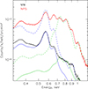 |
Fig. A.1. Spectrum of a large region inside the NPS (red points) in comparison with the typical "Milky Way" spectrum well outside the NPS (black points). Contributions of the detector background and CXB have been subtracted. The blue and green lines illustrate a few characteristic models. The solid blue line shows the APEC spectrum with the temperature Tw = 0.16 keV and abundance Z/Z⊙ = 0.05, using the abundance ratios from Asplund et al. (2009). The dashed blue line shows the same model with a three times larger abundance, i.e., Z/Z⊙ = 0.15. The solid green line shows the APEC model with the temperature Th = 0.5 keV, Z/Z⊙ = 0.05, and the emission measure multiplied by a factor of (Tw/Th)2. The dashed green line shows the same model with Z/Z⊙ = 0.7. A comparison of the histograms and the dashed lines shows that overabundances in the range 3-10 are needed to reproduce the enhanced brightness of the NPS compared to the Galaxy (assuming comparable pressures and linear sizes of the emitting regions). |
Appendix B: Plumes in 3D
In this section, we outline two simple scenarios for plume trajectories. In the first scenario, a plume is produced by a continuous source. The plume initially moves together with stars and gas in the disk and eventually joins the motion of the halo gas. In the second scenario, a trajectory of a massless buoyant bubble is considered.
B.1. Plumes from a moving source
The first case corresponds to the model described by Eqs. 1 and 2. Figure B.1 illustrates the shapes of the "plumes" in a stationary 3D frame. As the plume rises, it gradually joints the slowly rotating gas in the disk. By design, the rising plumes retain the same distance from the GC in projection to the disk.
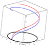 |
Fig. B.1. Example of a 3D trajectory of a plume rising above the disk according to Eqs. 1 and 2 and integrated over 140 Myr. Only one side of the plume is shown. The black circle depicts a circle in the disk plane with a radius of ∼5 kpc. The blue line corresponds to case (a), namely the source of the plume moves together with the gas and stars in the disk plane. The red curve is case (b), when the source of the plume, i.e., an area of active star formation, moves relative to the gas. At this distance from the GC, the difference between these two cases is not large. |
B.2. Trajectory of a massless buoyant bubble
Here we consider the trajectory of a single (massless) bubble moving in a stratified atmosphere of the Galaxy. Similarly to galaxy clusters (Gull & Northover 1973; Churazov et al. 2000), the velocity of the bubble is set by the balance of pressure gradients and the drag force acting on the bubble:
 (B.1)
(B.1)
where u is the 3D velocity vector of the bubble velocity with respect to the halo gas (u = |u|), ρ and P are the halo gas density and pressure, respectively, A and V are the area and volume of the bubble, and Cd is the appropriate drag coefficient (e.g., Zhang et al. 2018). The bubble size is assumed to be smaller than the pressure scale height and the velocity remains subsonic. For an atmosphere in hydrostatic equilibrium, 1/ρ∇P = −∇ϕ and, therefore, u can be directly calculated from the gravitational potential ϕ, which in our case can include a contribution from halo gas rotation. To this end, we used the approximation of the Milky Way potential from Barros et al. (2016), to which we added a centrifugal term (−Vh2lnR) for a cylindrical rotation, where R is the distance from the Milky Way center in the disk plane and Vh is the gas rotation velocity. The rotation velocity of the gas is added to u to get the bubble velocity in the nonrotating frame. The effects of rotation on the bubble trajectory are illustrated in Fig. B.2. This figure shows that different configurations are possible depending on the gas rotation pattern. The three solutions shown in the figure, cover the plausible range of halo rotations. For a nonrotating halo (green curve) the bubble moves along the potential gradient created by the Milky Way mass distribution. The blue and red lines cover the cases of moderate (100 km s−1) and extreme (200 km s−1) halo rotation speed. In particular, the case of the halo rotation velocity with ∼180 km s−1 (Hodges-Kluck et al. 2016) should be more close to the red curve. Of course, the rotation pattern can be much more complicated than the cylindrical pattern considered here.
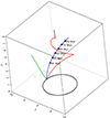 |
Fig. B.2. 3D trajectory of a (single) small and massless bubble rising under the action of buoyancy in a rotating but otherwise static atmosphere. The initial bubble is released at a distance of 5 kpc from the center (just above the disk plane). The green line shows the case of a nonrotating atmosphere. In this case, the bubble moves away from the Galaxy center in the disk and then switches to a more radial trajectory. The blue curve shows the case of a slowly rotating halo (Vh ∼ 100 km s−1). The bubble is now involved in rotation and motion towards larger radii. Finally, the red curve illustrates the case of fast rotation of the halo gas (Vh ∼ 200 km s−1). In this case, the centrifugal force is strong, and an inverted pressure gradient pushes the bubble closer to the rotation axis. |
We also emphasize that Fig. B.2 (unlike Fig. B.1) shows trajectories of individual "bubbles" rather than "plumes" that are formed by many bubbles released at different times. Assuming that the source of the bubbles is moving together with stars in the disk, the plume trajectories (a combination of bubbles released at different times) are shown in Fig. B.3. Qualitatively, they resemble the plumes shown in Fig. B.1, except for the presence of radial migration.
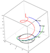 |
Fig. B.3. 3D trajectory of a sequence of bubbles (i.e., a plume). Individual bubbles follow the trajectories shown in Fig. B.2. The source of the bubbles moves with the same velocity as stars in the disk. Overall, plume trajectories are qualitatively similar to those shown in Fig. B.3. |
Set of "sources" used to illustrate typical trajectories of gaseous plumes in Fig. C.1.
Appendix C: Plumes’ trajectories as seen from the Sun
The 3D trajectories discussed above will be distorted once they are projected on the sky plane. In particular, the segments closer to the Sun are seen at higher latitudes than those on the opposite side of the Galaxy. The east and west segments also differ in shape due to rotation. This induces an asymmetry in the expected structures even if they have the same shape in 3D. This is illustrated in Fig. C.1, where projected trajectories are superposed onto sky maps in the radio-continuum band (top panel) and its polarized component.
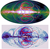 |
Fig. D.1. Trajectories of the gaseous plumes in Aitoff projection. Top: Sample trajectories of the gaseous plumes superposed on the radio continuum map at 408 MHz map (Haslam et al. 1981; Remazeilles et al. 2015). These trajectories correspond to an arbitrarily chosen set of plume "sources" (see Table B.1). Red and blue correspond to cases when sources have the same azimuthal velocity in the disk as stars. They correspond to the plume sources currently observed at a given Galactic longitude but different distances from the Sun: red and blue mark sources that are closer and farther away, respectively. White corresponds to sources that move with the pattern speed. Three properties of the trajectories are worth mentioning: (i) the "spirals" are warped in the central region of the Galaxy well above the plane, (ii) the east–west asymmetry set by the Galaxy rotation direction, and (iii) trajectories tend to overlap in certain regions of the sky even if they come from well-separated sources. Bottom: Polarized synchrotron emission map (e.g., Planck Collaboration IV 2020) with a subset of trajectories superposed. The circles correspond to time tags (every 30 Myr) in this model and are labeled. |
Appendix D: Enhanced metallicity of plumes
The enhanced metallicity of the NPS hot material enriched by supernovae is important for the proposed scenario. The thermal energy of the NPS Eth ∼ 2 × 1055 erg (see Sect. 4) suggests the explosion of Nsn ∼ 2 × 10⁴ core-collapse supernovae (CCSNe) with a typical kinetic energy of 1051 erg (the lifetime of a SFR is too short for supernovae Ia to explode). We rely on two sets of oxygen nucleosynthesis calculations for CCSN progenitors in the range of 11 - 40M⊙ by (Woosley & Weaver 1995, hereafter WW95) and (Kobayashi et al. 2006, hereafter K06). In K06, the data on 11M⊙ progenitors are lacking. We, therefore, adopt the ejected mass of oxygen from WW95 for this particular progenitor. The abundance of other elements relative to oxygen is assumed to follow (approximately) the solar composition.
The average mass of ejected oxygen per CCSN (mO) is inferred assuming Salpeter initial mass function dN/dm ∝ m−2.35 in the mass range of 0.1 – 100M⊙. We find comparable values of mO, 2.2M⊙ and 2.6M⊙, for WW95 and K06 data, respectively. The average mO = 2.4M⊙ multiplied by the CCSN number Nsn provides us with the total amount of oxygen synthesized by supernovae of the SFR MO ≈ 5 × 10⁴ M⊙. The synthesized oxygen mixed with the gas of the solar composition (solar abundance X(O)⊙ = 0.01) produces enhanced overall metallicity. The total mass of the mixture (Mhot) is fixed by the thermal energy of the X-ray-emitting gas Eth = (5/2)kTxMhot/(μmp). For the average molecular weight μ = 0.61 and temperature kTx = 0.6 keV one obtains Mhot = 4 × 10⁶ M⊙. The expected oxygen abundance of the NPS hot gas is then X(O) = X(O)⊙ + MO/Mhot ≈ 0.02, twice the solar value.
The effect of the enhanced oxygen abundance of the NPS can be expressed formally as X(O) = X(O)⊙(1 + y) with the factor y responsible for the synthesized oxygen and estimated for the NPS to be about unity. Let the abundance of a certain element (El) relative to oxygen produced by CCSNe with respect to the solar abundance is ϕ = (El/O)/(El/O)⊙. The overabundance factor of this element with respect to solar in the NPS material, assuming the initial abundance in the SFR to be solar, is then f = 1 + yϕ.
The relative abundances ϕ of key elements, viz. C, N, Ne, Mg, Si, S, and Fe, generated by the CCSNe, can be derived from spectroscopic stellar data of [El/Fe] = log(El/Fe)–log(El/Fe)⊙ for metal-poor stars ([Fe/H] < -2), in which metallicity domain the nucleosynthesis by CCSNe dominates. We rely on [El/Fe] versus [Fe/H] data compiled by Kobayashi et al. (2020). For C and N the scatter of [El/Fe] values relative to the average for different stars is very large, of ∼0.5 dex; in other cases, the scatter is of 0.2–0.3 dex. Anyway, for each element we obtain an average value of [El/Fe] with a typical error of 0.1 dex, which is converted to ϕ with a relative error of ≈20%. In the case of Ne, lacking stellar data, we rely on the theoretical prediction that CCSNe nucleosynthesis results in the solar ratio of Ne/O (Kobayashi et al. 2020). For the adopted value of y = 1, the estimated overabundance factors in the NPS material turn out to be f = 1.5 for C, N, and S, f = 1.6 for Mg and Si, f = 2 for O and Ne, and f = 1.25 in the case of Fe – all factors with a relative error of approximately 20%.
Appendix E: The chimney model
The clustering of CCSNe produced at the end of the evolution of massive stars in OB associations and compact clusters has a profound effect on the ISM and the galactic ecology (Mac Low & McCray 1988; Heiles 1990; de Avillez 2000; Kim et al. 2020). Multiple correlated supernovae and the powerful winds of OB stars create superbubbles and eventually (for powerful enough systems) produce the chimney-type structures (Norman & Ikeuchi 1989). We consider such superbubbles as potential sources of the plumes. To study the effect of the galactic magnetic field on the superbubble breakthrough from the disk to halo Tomisaka (1998) performed 3D MHD simulations for different assumptions on the large-scale magnetic field structure. The magnetic field with the strength of ∼ 5 μG with a broad kiloparsec-scale height can confine a superbubble of a modest kinetic luminosity 3×1037 erg s−1 for about 20 Myr within the scale height of ∣z ∣ ∼300 pc from the disk, while in a model with the field that follows the scaling B ∝ ρ1/2 (with the mid-plane field magnitude of 5 μG) the superbubble blows out to the halo. The evolution of superbubbles in density stratified disks that blow out into galactic halo may be a subject of Rayleigh-Taylor instabilities (Baumgartner & Breitschwerdt 2013; Schulreich & Breitschwerdt 2022). A parsec-resolution multiphase simulation of the local star-forming galactic disk with the account for supernova feedback effects revealed that the hot galactic outflows (with gas temperatures above 106 K) may carry about 10%-20% of the energy and 30%-60% of the metal mass injected by supernovae (Kim et al. 2020). These values are broadly consistent with the energy requirements needed to produce the X-ray plumes discussed in the text.
Nonthermal particles accelerated by shocks from supernovae and stellar winds at the active phase of the evolution of superbubble which is about 10 Myr (Bykov 2014). Then relativistic particles will be blown out to the low halo with the frozen-in magnetic fields of the chimney-type plasma outflow. Relativistic electrons of energy ∼ 100 GeV would have in the halo a lifetime of about 10 Myr due to synchrotron-Compton losses and will radiate in magnetic fields of a few microgauss at frequencies of ≲ 50 GHz. The synchrotron-Compton cooling time for the relativistic electron of energy ℰGeV (measured in GeV) in the galactic halo can be estimated as
 (E.1)
(E.1)
Appendix F: The role of W43
Here we discuss in brief the mini-starburst complex W 43 as a prototype powerhouse located in the Galactic molecular ring assuming that an ensemble of such complexes may supply the plumes over a long period of approximately a hundred million years. The molecular complex W 43 with the estimated mass ∼7 × 10⁶ M⊙ is presumably located at the connecting point of the Scutum-Centaurus Galactic arm and the Galactic bar (Nguyen Luong et al. 2011). W 43 excited a giant H II region dubbed NGC 3603. The equivalent diameter of the coherent complex of molecular clouds is ∼140 pc and it is surrounded by an atomic gas envelope of about two times larger diameter. Nguyen Luong et al. (2011) noted that the transition from circular to elliptical orbits in the spiral arm and bar potentials might cause high-velocity streams and thus efficient star formation episodes of current rate at least ∼0.01 M⊙ yr−1 as estimated from 8 μm luminosity measurements but it is likely increasing to ∼0.1 M⊙ yr−1. On longer timescales (∼ 100 Myr), multiple episodes of high star formation rate can be expected from colliding molecular clouds entrained by the large scale streams.
The giant HII region NGC 3603, which is associated with the complex, produces the Lyman continuum photon rate of about 4 × 1051 photons s−1 and is the most powerful HII region in the Galaxy (De Buizer et al. 2024). A compact dense cluster of young massive stars HD 97950 (also known as W 43 cluster) powering NGC 3603 has an estimated dynamic stellar mass of 18,000 M⊙ including more than 70 O and 3 Wolf-Rayet stars. The distance to the powerful starburst region NGC 3603 of 7.2 ± 0.1 kpc was estimated by Drew et al. (2019) from Gaia Data Release 2 stellar parallax measurements (see also De Buizer et al. 2024 for a recent discussion). From the Very Long Baseline Array trigonometric parallax measurements of masers toward W43 Zhang et al. (2014) derived a distance of 5.49 kpc to the complex (see also Li et al. 2022, for another distance estimate of ∼4.8 kpc). The origin and ages of molecular clumps and stellar population in NGC 3603 are still the subject of debate De Buizer et al. (2024). ALMA observations revealed that the core mass function in W43-MM1 is much shallower in the high-mass range than the standard initial mass function (Motte et al. 2018). Fukui et al. (2014, 2021) discussed the formation of cluster W 43 due to a collision of two molecular clouds about 1 Myr ago. This age is consistent with that of the highest mass stellar population in the cluster. The suggestion by Nguyen Luong et al. (2011) about the origin of the star-forming complex W 43/NGC 3603 due to the collision of molecular clouds following their circular orbits in the Scutum-Centaurus arm and the clouds at the elliptical orbits of the Galactic bar makes the complex W 43 as well as other complexes along the Molecular Ring where the Galactic arms meet the bar to be favorable locations for the intense star formation episodes in the past.
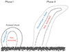 |
Fig. F.1. Possible formation scenario of a NPS-like structure. During the initial phase after the breakout (left), a shock driven by the hot and metal-rich gas of a superbubble propagates through the ambient gas. At later stages (right) the gas is stretched and bent into a plume but possibly maintains the layered structure. |
Very high energy emission source HESS J1848-018 (H.E.S.S. Collaboration 2018) can possibly be associated with W 43. From Fermi Large Area Telescope detection of extended high energy gamma-ray source source in the direction of W 43 Yang & Wang (2020) estimated the total cosmic ray energy within the source to explain the detected flux to be (2.3 ± 0.3)×1048 erg.
All Tables
Set of "sources" used to illustrate typical trajectories of gaseous plumes in Fig. C.1.
All Figures
|
Fig. 1. X-ray and radio images of the NPS region. Left and middle panels: 0.52−0.61 keV and 0.7−0.96 keV eROSITA X-ray images, respectively. For comparison, the right panel shows the 408 MHz radio image from the all-sky continuum surveys (Haslam et al. 1981; Remazeilles et al. 2015). The images in galactic coordinates are shown in stereographic projection for a better view of the regions near the Galactic plane and the Galactic north pole. The X-ray images are particle-background-subtracted and exposure-corrected. The brightest compact sources and galaxy clusters have been masked, and the resulting image convolved with σ = 20′ Gaussian. Still prominently visible in the image are RS Oph (bright dot near the bottom of the left image) and the stray light halo around Sco X-1 (at the right edge of the middle image). The dashed white lines show the wedge used to extract radial profiles. The numbers indicate the distance (in degrees) from the wedge center, which is at (l, b) = (338 ° ,32 ° ) in Galactic coordinates. |
| In the text | |
|
Fig. 2. Radial profiles of the NPS X-ray emission. Left: Observed surface brightness in several energy bands. The wedge used for the flux extraction is shown in Fig. 1. The bright edge of the NPS is at x ≈ 48°. The contributions of the instrumental background and distant (unresolved) sources composing cosmic X-ray background (CXB) have been subtracted, leaving only the flux from the Galaxy. Right: Same as the left plot, but after subtracting the mean level at x = 60 − 70°, re-normalizing by the flux at x = 35°, and lightly smoothing with a Gaussian filter (σ = 0.4°). In addition, the radio surface brightness profile (Haslam, 408 MHz) after applying the same procedure (subtraction, re-normalization, and smoothing) is shown with the dashed red curve. |
| In the text | |
|
Fig. A.1. Spectrum of a large region inside the NPS (red points) in comparison with the typical "Milky Way" spectrum well outside the NPS (black points). Contributions of the detector background and CXB have been subtracted. The blue and green lines illustrate a few characteristic models. The solid blue line shows the APEC spectrum with the temperature Tw = 0.16 keV and abundance Z/Z⊙ = 0.05, using the abundance ratios from Asplund et al. (2009). The dashed blue line shows the same model with a three times larger abundance, i.e., Z/Z⊙ = 0.15. The solid green line shows the APEC model with the temperature Th = 0.5 keV, Z/Z⊙ = 0.05, and the emission measure multiplied by a factor of (Tw/Th)2. The dashed green line shows the same model with Z/Z⊙ = 0.7. A comparison of the histograms and the dashed lines shows that overabundances in the range 3-10 are needed to reproduce the enhanced brightness of the NPS compared to the Galaxy (assuming comparable pressures and linear sizes of the emitting regions). |
| In the text | |
|
Fig. B.1. Example of a 3D trajectory of a plume rising above the disk according to Eqs. 1 and 2 and integrated over 140 Myr. Only one side of the plume is shown. The black circle depicts a circle in the disk plane with a radius of ∼5 kpc. The blue line corresponds to case (a), namely the source of the plume moves together with the gas and stars in the disk plane. The red curve is case (b), when the source of the plume, i.e., an area of active star formation, moves relative to the gas. At this distance from the GC, the difference between these two cases is not large. |
| In the text | |
|
Fig. B.2. 3D trajectory of a (single) small and massless bubble rising under the action of buoyancy in a rotating but otherwise static atmosphere. The initial bubble is released at a distance of 5 kpc from the center (just above the disk plane). The green line shows the case of a nonrotating atmosphere. In this case, the bubble moves away from the Galaxy center in the disk and then switches to a more radial trajectory. The blue curve shows the case of a slowly rotating halo (Vh ∼ 100 km s−1). The bubble is now involved in rotation and motion towards larger radii. Finally, the red curve illustrates the case of fast rotation of the halo gas (Vh ∼ 200 km s−1). In this case, the centrifugal force is strong, and an inverted pressure gradient pushes the bubble closer to the rotation axis. |
| In the text | |
|
Fig. B.3. 3D trajectory of a sequence of bubbles (i.e., a plume). Individual bubbles follow the trajectories shown in Fig. B.2. The source of the bubbles moves with the same velocity as stars in the disk. Overall, plume trajectories are qualitatively similar to those shown in Fig. B.3. |
| In the text | |
|
Fig. D.1. Trajectories of the gaseous plumes in Aitoff projection. Top: Sample trajectories of the gaseous plumes superposed on the radio continuum map at 408 MHz map (Haslam et al. 1981; Remazeilles et al. 2015). These trajectories correspond to an arbitrarily chosen set of plume "sources" (see Table B.1). Red and blue correspond to cases when sources have the same azimuthal velocity in the disk as stars. They correspond to the plume sources currently observed at a given Galactic longitude but different distances from the Sun: red and blue mark sources that are closer and farther away, respectively. White corresponds to sources that move with the pattern speed. Three properties of the trajectories are worth mentioning: (i) the "spirals" are warped in the central region of the Galaxy well above the plane, (ii) the east–west asymmetry set by the Galaxy rotation direction, and (iii) trajectories tend to overlap in certain regions of the sky even if they come from well-separated sources. Bottom: Polarized synchrotron emission map (e.g., Planck Collaboration IV 2020) with a subset of trajectories superposed. The circles correspond to time tags (every 30 Myr) in this model and are labeled. |
| In the text | |
|
Fig. F.1. Possible formation scenario of a NPS-like structure. During the initial phase after the breakout (left), a shock driven by the hot and metal-rich gas of a superbubble propagates through the ambient gas. At later stages (right) the gas is stretched and bent into a plume but possibly maintains the layered structure. |
| In the text | |
Current usage metrics show cumulative count of Article Views (full-text article views including HTML views, PDF and ePub downloads, according to the available data) and Abstracts Views on Vision4Press platform.
Data correspond to usage on the plateform after 2015. The current usage metrics is available 48-96 hours after online publication and is updated daily on week days.
Initial download of the metrics may take a while.