| Issue |
A&A
Volume 698, June 2025
|
|
|---|---|---|
| Article Number | A313 | |
| Number of page(s) | 14 | |
| Section | Galactic structure, stellar clusters and populations | |
| DOI | https://doi.org/10.1051/0004-6361/202554389 | |
| Published online | 27 June 2025 | |
Disentangling the Galactic centre X-ray reflection signal using XMM-Newton data
1
Center for Astrophysics | Harvard & Smithsonian,
60 Garden Street,
Cambridge,
MA
02138,
USA
2
INAF-Osservatorio Astronomico di Palermo,
Piazza del Parlamento 1,
90134
Palermo,
Italy
3
Universitäts-Sternwarte, Fakultät für Physik, Ludwig-Maximilians Universität,
Scheinerstr. 1,
81679
München,
Germany
4
Max Planck Institute for Astrophysics,
Karl-Schwarzschild-Str. 1,
85741
Garching,
Germany
5
Space Research Institute (IKI),
Profsoyuznaya 84/32,
Moscow
117997,
Russia
6
INAF-Osservatorio Astronomico di Brera,
Via E. Bianchi 46,
23807
Merate (LC),
Italy
7
Max-Planck-Institut für extraterrestrische Physik,
Gießenbachstraße 1,
85748,
Garching,
Germany
8
Como Lake Center for Astrophysics (CLAP), DiSAT, Università degli Studi dell’Insubria,
via Valleggio 11,
22100
Como,
Italy
★ Corresponding author: This email address is being protected from spambots. You need JavaScript enabled to view it.
Received:
5
March
2025
Accepted:
2
May
2025
Abstract
Aims. We investigate the X-ray emission from the Galactic centre (GC) region, focusing on the 6.4 keV fluorescent line of neutral or weakly ionised iron, which is commonly attributed to X-ray reflection from dense molecular clouds. Our goal is to separate the reflection signal from other physical X-ray components. We aim to produce a clean map of the 6.4 keV emission, thus providing a better understanding of the X-ray reflection processes in the GC.
Methods. We utilised a deep mosaic of all available XMM-Newton observations, encompassing the central 40 square degrees of the Galaxy. This dataset integrates information from 503 individual observations, resulting in a total clean exposure time of 7.5 Ms. The mosaics of two narrow bands centred at 6.7 keV and 6.4 keV, and a broader continuum band at lower energies (5−6.1 keV), provided valuable spatial and spectral information on the X-ray emission. These combined with the stellar mass distribution of our Galaxy enabled us to decompose the observed signal into physically meaningful components.
Results. Our analysis shows that the cleaned 6.4 keV band map, free from the contribution of bright and unresolved point sources, is predominantly shaped by X-ray reflection from dense molecular clouds. The spatial distribution of this emission, which strongly correlates with the molecular gas distribution in the central molecular zone (CMZ), supports the interpretation that this map provides the best estimate of the X-ray reflection signal averaged over the last two decades. This cleaned reflection map could serve as a tool for future studies aiming to quantify upper limits on the reflection contribution from low-energy cosmic rays in unilluminated regions. Moreover, we estimate that, on average, within the CMZ, approximately 65% of the ridge emission contributes to the observed emission in the 6.4 keV band, a factor that should be incorporated into upcoming investigations of the GC, such as polarisation studies of the reflected X-ray continuum from molecular clouds and statistical assessments of the reflection surface brightness.
Key words: ISM: clouds / Galaxy: bulge / Galaxy: center / Galaxy: disk / X-rays: general / X-rays: ISM
© The Authors 2025
 Open Access article, published by EDP Sciences, under the terms of the Creative Commons Attribution License (https://creativecommons.org/licenses/by/4.0), which permits unrestricted use, distribution, and reproduction in any medium, provided the original work is properly cited.
This article is published in open access under the Subscribe to Open model. This email address is being protected from spambots. You need JavaScript enabled to view it. to support open access publication.
1 Introduction
The Galactic centre (GC), the central few degrees of our Galaxy, is an environment of very energetic phenomena (i.e. the flaring activity of Sgr A*, numerous supernova explosions, stellar winds of massive stars, active stars, and various types of X-rays binaries) that result in the emission of soft (<4 keV) as well as hard X-rays (>4 keV; for reviews, see Ponti et al. 2013; Koyama 2018). This environment makes the GC region rich in (apparently) diffuse X-ray emission. In particular, in hard X-rays, two components are commonly invoked to describe the spectral and spatial properties of the emission: the Galactic ridge X-ray emission and the reflected X-ray emission from the massive molecular clouds.
The Galactic ridge X-ray emission has been traced by the ∼6.7 keV line, which originates from He-like iron (Fe XXV) and indicates the existence of very hot gas (3−10 keV; e.g. Cooke et al. 1969; Worrall et al. 1982; Koyama et al. 1986, 2007; Yamauchi & Koyama 1993; Revnivtsev et al. 2009). If this hot plasma is bound to compact objects, the spatial distribution of the ridge X-ray emission is expected to follow the smooth distribution of the stellar mass along our Galaxy, including separate contributions of the Galactic disc and bar, the nuclear stellar disc (NSD), and the nuclear star cluster (NSC). Its spectral shape is relatively well established in regions outside the GC and in the hard X-ray band up to ∼60 keV (e.g. Krivonos et al. 2007; Yuasa et al. 2012; Krivonos et al. 2025). However, in the very central two degrees of our Galaxy, the origin of the 6.7 keV emission has been widely debated as it was found in excess of what was expected by the stellar mass distribution (SMD) of the Galaxy. This excess emission is attributed to unresolved point sources (a result of a new or larger population of known systems), true hot plasma (due to past activity of Sgr A* or past supernova explosions), or a combination of the two (e.g. Koyama et al. 1989; Yamauchi & Koyama 1993; Muno et al. 2004; Park et al. 2004; Revnivtsev et al. 2007; Uchiyama et al. 2011; Nishiyama et al. 2013; Heard & Warwick 2013). Therefore, in the central few degrees of the Galaxy, the spectrum of the Galactic ridge X-ray emission remains uncertain due to the challenge of disentangling diffuse emission from unresolved point sources and the fact that it likely arises from a spatially variable mixture of populations of point sources (accreting white dwarfs and stars; e.g. Revnivtsev et al. 2006a, 2009; Xu et al. 2016). Anastasopoulou et al. (2023) find that the observed GC X-ray excess might be the result of higher X-ray emissivity per unit stellar mass in the GC, possibly owing to higher metallicity in the GC (e.g. Yamauchi et al. 2016; Feldmeier-Krause et al. 2017; Zhu et al. 2018; Do et al. 2018; Schultheis et al. 2021; Fritz et al. 2021). Anastasopoulou et al. (2023) also find a remarkable similarity between the X-ray emission and the stellar mass density distribution in the GC when scaling for the higher X-ray emissivity in the NSD and NSC, while a small remaining excess in the central 0.3 degrees of the GC can be explained by the contribution of supernova remnants based on the measured supernova rate.
The spectrum of the reflected X-ray emission, dominated by a ∼6.4 keV line originating from neutral or weakly ionised iron (Fe Kα), can be readily predicted and indicates the existence of cold gas. However, its spatial distribution is complicated. In the central degrees of the GC, the region known as the central molecular zone (CMZ), the emission from the 6.4 keV line has been found to be asymmetric (in contrast with the more or less uniform distribution of the Galactic ridge X-ray emission) and to be correlated spatially with GC molecular clouds, which are also highly asymmetrically distributed, with approximately three-quarters found at positive longitudes (Bally et al. 1988). The main mechanism of its production is considered to be X-ray reflection off dense molecular clouds, which act as mirrors to the past flaring activity of the central supermassive black hole Sgr A* on timescales of hundreds of years (e.g. Sunyaev et al. 1993; Koyama et al. 1996; Ponti et al. 2013; Churazov et al. 2017a; Khabibullin et al. 2022). Studying the X-ray reflection from molecular clouds in detail has significantly enhanced our understanding of the type and the position of the illuminating source and its variability (e.g. Ponti et al. 2010; Clavel et al. 2013; Terrier et al. 2010; Chuard et al. 2018; Kuznetsova et al. 2022; Stel et al. 2025). In addition to reflection, other mechanisms could account for the observed continuum and the 6.4 keV emission line in the CMZ. One such mechanism is collisional ionisation from accelerated particles (cosmic ray electrons, protons, and ions; e.g. Valinia et al. 2000; Yusef-Zadeh et al. 2002, 2007; Bykov 2002; Dogiel et al. 2009), which was initially proposed to be the case for emission in molecular gas around the Arches cluster as no variability had been observed over an eight-year period (e.g. Wang et al. 2006; Capelli et al. 2011). However, recent studies have shown significant variability around the Arches cluster over a 20-year span, with some residual emission still possibly attributable to cosmic rays (e.g. Clavel et al. 2014; Krivonos et al. 2017; Chernyshov et al. 2018; Kuznetsova et al. 2019; Stel et al. 2025). Observations of fast flux variations in the 6.4 keV-emitting clouds (e.g. Muno et al. 2007; Ponti et al. 2010; Capelli et al. 2012; Clavel et al. 2013; Churazov et al. 2017b; Inui et al. 2009; Terrier et al. 2010; Ryu et al. 2013; Chuard et al. 2018) and polarisation (Churazov et al. 2017a; Marin et al. 2023) are evidence against a cosmic-ray-induced Fe Kα origin, at least for the variable component of the emission (see the review by Ponti et al. 2013).
Several studies have concluded that point sources contribute minimally to the 6.4 keV emission in the GC. For instance, Murakami et al. (2001), using a 100 ks Chandra observation of the central 3 × 3.5 arcmin region of the Sgr B2 molecular cloud, resolved approximately 18 sources, which account for only 3% of the luminosity produced by reflection. Moreover, Wang et al. (2002) used Chandra data to map the central degrees of the GC, and by extracting composite spectra of the resolved point source population, confirmed that these sources contribute minimally to the 6.4 keV emission. However, they showed that these sources account for most of the observed 6.7 keV emission. On the other hand, very deep ∼1 Ms Chandra observations of the Galactic ridge and the GC (Revnivtsev et al. 2007, 2009) have shown that a substantial portion of the 4−8 keV energy range is contributed by faint sources. Astrophysical objects like low-mass X-ray binaries and various types of cataclysmic variables are known to produce strong 6.4 keV emission lines, primarily from the inner regions of their accretion discs and reflection from the white dwarf surface (e.g. Kallman & White 1989; Barret et al. 2000).
In this work, we combine spatial and spectral information on the X-ray emission provided by the deep XMM-Newton mosaic of the GC and inner Galactic disc region in order to decompose the signal into physically motivated components. Namely, using the spatial correlations of the continuum, the 6.7 keV and 6.4 keV bands, together with the models of the stellar distribution in this region, we derived a ‘residual’ 6.4 keV emission map, which we argue provides the best estimate for the X-ray reflection signal in the GC.
This paper is organised as follows: In Sect. 2 we describe the XMM-Newton observations comprising the big mosaic and the SMD models, and in Sect. 3 we present the method we used to produce the clean reflection emission maps. In Sect. 4, we present and discuss our results and compare them with known maps of molecular clouds in the GC. Finally, we provide our conclusions in Sect. 5.
2 Data
2.1 X-ray data
For this project we used all XMM-Newton observations available up to 25 February 2024 (503; ∼7.5 Ms clean – background flare- and vignetting-corrected – exposure time EPIC-pn equivalent) with exposure times greater than 5 ks and within the central 40 square degrees of our Galaxy. The list of observations is reported in Anastasopoulou et al. (2023), Ponti et al. (2019), and Ponti et al. (2015). The information of the most recent 133 observations are reported in Table A.1.
The calibration and analysis of the observations was performed using the standard tools of the XMM-Newton Science Analysis System (SAS) v21.0.0, and is reported in detail in Anastasopoulou et al. (2023). The final product of the analysis is a stray-light free, background subtracted, source excised, and adaptively smoothed mosaic for each XMM-Newton detector, and each energy band of interest. The MOS and pn mosaics were combined accounting for the effective area differences between the detectors at the corresponding energy band (details available in the appendix of Anastasopoulou et al. 2023). To isolate the fluorescent Fe K emission from other contaminating processes in the GC, we produced mosaics for three XMM-Newton energy bands, 6.3−6.5 keV (X64), 6.62−6.8 keV (X67), and 5.0−6.1 keV (X50). The mosaics in this work are always presented in units of counts per second per pixel (cr/pix), with each pixel measuring 8 × 8 arcseconds. These bands represent the Fe XXV from very hot plasma, the neutral or weakly ionised Fe Kα fluorescent emission, and the continuum at lower energies, respectively. The spectral shape of each component is shown in Fig. 1 where the X67 band is intentionally slightly offset from the 6.7 keV line peak to minimise contamination from the nearby 6.4 keV fluorescent line. The central regions (∼8 × 1 degrees) of the raw mosaics at each band are presented in the first three panels of Fig. 2.
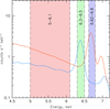 |
Fig. 1 Spectral representation of the three energy bands used in this project. The bands are highlighted by the shaded regions. The representative model spectra (convolved with the XMM-Newton spectra response function) of hot plasma (apec model in XSPEC) and reflection (crefl16 model; Churazov et al. 2017b) are shown as orange and blue lines, respectively. |
2.2 Stellar mass distribution model
The total stellar density of the Milky Way can be represented as a sum of distinct components:

These components, arranged by increasing Galactocentric radius R, include:
The NSC, a dense and slightly flattened structure of stars, surrounding Sgr A* with a mass ≈ 2.5 × 10⁷ M⊙, dominating within R ≲ 10 pc (Schödel et al. 2014; Neumayer et al. 2020).
The NSD, a flattened distribution with a mass of approximately 1.05 × 10⁹ M⊙, prevalent at 10 ⩽ R ⩽ 200 pc (Launhardt et al. 2002; Sormani et al. 2022b).
The Galactic bar, an elongated structure in the Galactic plane (GP) with a mass near 1.9 × 10¹⁰ M⊙, which dominates within 0.2 ≲ R ≲ 3 kpc (Bland-Hawthorn & Gerhard 2016).
The Galactic disc, which is the main contributor to the stellar mass density beyond R ≳ 3 kpc.
The SMD model of our Galaxy is created by combining recent models of each individual component. For this project we used the components described as Model 2 in Table 2 and Sect. 2.2 of Anastasopoulou et al. (2023). Namely, for the NSC we used the best-fitting model from Chatzopoulos et al. (2015)1, for the NSD the fiducial model of Sormani et al. (2022b), for the Galactic bar the bar + long bar from Sormani et al. (2022a), which is based on the numerical models by Portail et al. (2017), and for the Galactic Disc the disc from Sormani et al. (2022a). The SMD model, calculated by integrating the volume density (ρ(x, y, z)) along the line of sight to obtain the surface density on the plane of the sky (∑(l, b) where l and b are the Galactic coordinates), is shown in the bottom panel of Fig. 2.
3 Method
The GP is densely populated with many different objects (and classes of objects). It is therefore not surprising that from any location in the GP, we almost always see a composite X-ray spectrum that includes contributions of many unrelated objects along the same line of sight. There are many ways of emphasising one particular component. These range from selecting an energy band, where this component is expected to dominate, to fitting a multi-component spectral model for each sky position. The former is very simple but usually results in a map that can be severely contaminated by other components, while the latter might be too complicated and lead to noisy results if the spectral model is non-linear. One can partially mitigate the noise problem by resorting to linear spectral models (see Churazov et al. 2017b for a two-component case), which works well if the spectral shapes of different components are known. In this case, their normalisations can be independently determined at every position via a linear combination of data. A similar approach can be applied to a collection of maps as is often done in the analysis of cosmic microwave background data (e.g. Planck Collaboration XXII 2016). For a known spectral shape, one can predict the contribution of the component j with amplitude Aj(x, y) to any map i, i.e. mi(x, y)=Σj Aj(x, y) sj, i. For instance, if Aj(x, y) is a surface density of sources of type j, for example stars, their contribution to the X-ray map mi(x, y) in the band i is set by the flux sj, i such sources produce in this band. Therefore, knowing sj, i one can select the coefficients αi so that a linear combination of maps m(x, y)=Σi αi mi(x, y) will eliminate some of the spectral components exactly and preserve the normalisation of the component of interest (at least for the noise-free data). A more practical version of the same procedure is to keep only the requirement of preserving the normalisation of one spectral component and then choose the coefficients so that the resulting map has the smallest L2 norm ∫ m2(x, y)dxdy. If the component of interest is confined to one particular band, i.e. s0, i = 0 for i ≠ 0, the above procedure reduces to finding the coefficient αi that minimise the norm:
![Mathematical equation: $\min _{\alpha} \Sigma_{x, y}\left[\frac{m_{0}(x, y)-\Sigma_{i} \alpha_{i} m_{i}(x, y)}{\sigma_{0}(x, y)}\right]^{2},$](/articles/aa/full_html/2025/06/aa54389-25/aa54389-25-eq2.png) (1)
(1)
where m0(x, y) is the reference map containing the component of interest (and the contributions of other components too),  is the estimated variance at a given position of the reference map (if it is known and other maps are free from the noise), and mi(x, y) for i = 1, N are the all other available maps. In this case, the maps need not be X-ray images but could be any images from other bands or models.
The shortcomings and limitations of the above approach are obvious. However, if strong spatial variations of different components are present, this procedure could reveal the level of correlations between the maps and, potentially, clean the maps from some of the contaminating signals. The method we used, compared to equivalent width (EW) approaches, is not biased by regions with low SMD, which can artificially increase the EW due to reduced continuum flux. Our method is less sensitive to variations in the SMD and provides a more accurate representation of the clean 6.4 keV emission, enabling a direct comparison with the dense gas distribution in the GC. In what follows we make another simplifying assumption by setting σ0(x, y) = 1. Effectively, this means that the algorithm minimises the variance of the residual image after removing the contributions of all components. This is a reasonable choice since we are dealing with smoothed images and mask regions heavily affected by systematics.
Our set of maps, presented in the previous sections, is summarised in Table 1. This study is focused on the X-ray map X64. This map contains the fluorescent line of neutral (or weakly ionised) iron. Other maps serve as possible proxies for various components, which may spatially correlate with our primary maps potentially revealing the origin of the emission (Anastasopoulou et al. 2023). We utilised two distinct maps to represent the SMD across our Galaxy. The first, labelled N, includes contributions from the NSC and the NSD. The second map, labelled B, accounts for contributions from the Galactic bar and the Galactic Disc. These components (N and B) are analysed separately to account for differences in X-ray emissivity between them, as highlighted in Anastasopoulou et al. (2023).
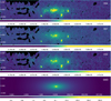 |
Fig. 2 Raw maps used in this study. From top to bottom: the XMM-Newton 6.4 keV (X64), 6.7 keV (X67), the continuum band (X50), and the SMD. The XMM-Newton maps are measured in count per second per pixel (cr/pix), whereas the SMD map represents stellar density in 103 M⊙/pix. The colour bar ranges are selected arbitrarily to emphasise and display morphological differences. The x-axis and y-axis represent the Galactic longitude and latitude, respectively, in degrees. |
Inclusion and exclusion regions
Our primary goal is to study the origin of the (apparently) diffuse emission by studying its spatial correlation with other components. From this point of view, the emission from bright X-ray sources is the source of contamination. While the bright point sources have already been excluded during the map-making process, some residual traces are present most probably due to dust scattering halos around these sources (e.g. Jin et al. 2017, 2018). For that reason, we applied an additional mask containing a list of regions (Table 2) including bright sources located within these areas. Part of the bright-source mask is shown in Fig. 3 with cyan circles.
Also, as explained in the previous section, the basic assumption is that physically unrelated signals are expected to be spatially uncorrelated. This is likely not true for the GC region, as the density of all classes of sources increases towards the centre of the Milky Way. To partially mitigate this problem, we additionally calculated all correlation coefficients for the entire extent of the map after masking the central region (ellipse shown in Fig. 3) that contains much of the gradient in the surface density of stars or other objects. Masking the central regions is particularly important because most of the molecular clouds that can be sources of ‘reflected’ emission are located there (see Sect. 4.1). In the next sections, we apply this technique to the X64 map obtained by XMM-Newton.
Set of maps used in the analysis.
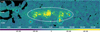 |
Fig. 3 Example of the cleaned X64 band map (X64 minus C-X67-X50). The mask is shown as a dashed ellipse, and solid circles correspond to bright sources. The map is in units of counts per second per pixel. Black regions indicate areas with no exposure, which may result from the removal of point sources, stray-light artefacts, or chip gaps. |
4 Results and discussion
4.1 Accounting for different contaminating components
Using the method outlined in Sect. 3, we calculated the contributions of all potential components (listed in Table 1) to the X64 map. This analysis is presented for the combined masking of the elliptical central region and bright sources, as it yielded significantly better results compared to using the bright source mask alone, which led to prominent negative residuals (briefly discussed in Appendix B). In Table 3 we present the best-fit coefficients for all possible combinations of the model X64-(C+c1N+c2B+c3X67+c4X50), and in Table 4 we summarise the different component combinations and the corresponding ratio of the final map variance to the initial map variance for the pixel values across the image. The variance provides a measure of how much noise is reduced after processing the image, such as masking bright sources or regions. However, it is important to note that real astrophysical features, can also contribute to an increase in the variance. Therefore, both noise reduction and the potential contribution of physical structures must be carefully considered when interpreting variance changes.
Overall, we find that the residuals for the C-N-B model are slightly lower than those for the C-N model. The lowest variance results are obtained by removing either the C-X67-X50 or C-N-B-X67-X50 components (Table 4). When we apply the best-fit coefficients to the entire map, we obtain no negative residuals, only slight residuals near very bright sources (Fig. 3).
To quantify further the differences between the various components, we extracted latitudinal and longitudinal profiles from the corresponding maps (Fig. 4). The profiles represent average values within a 0.5-degree width centred on Sgr A*. We present the latitudinal profiles along the central 1.2 degrees and longitudinal profiles along the central 4 degrees. We do not show regions farther from the centre, since there the profiles converge showing emission values close to zero. Regions containing bright sources (listed in Table 2) were masked prior to extracting the profiles. Including these regions resulted in numerous bright peaks, complicating the interpretation of the results. We observe that all models differ slightly, with models C-N and C-N-B-X67-X50 showing slight negative values particularly along the longitudinal profile (bottom panel of Fig. 4). The models with the smaller residual noise are C-N-B-X67-X50 and C-X67-X50. Of the two, we chose C-X67-X50 as the fiducial model since it exhibits no negative residuals.
Model C-N-B, represented by the dotted green line in Fig. 4, has an important application, as the cleaned X64 map is obtained solely by subtracting the SMD model contribution. This allows one to use the best-fit coefficients from Table 3 along with the analytical model in Sect. 2.2 to estimate the ‘non-reflection’ component contributing to the 6.4 keV band. Following Table 3, this component is given by (1.13 + 7.15N + 2.79B) × 10−7 cr/pix, where the N component, corresponding to the GC region, yields a 6.3−6.5 keV luminosity2 per unit stellar mass of LX[6.3−6.5, stellar] ∼1.3 × 1026 erg s−1  . For comparison, Revnivtsev et al. (2006b) report a 3−20 keV luminosity per stellar mass of (3.5 ± 0.5) × 1027 erg s−1
  , which corresponds to LX[6.3−6.5, apec] ∼ (6 ± 1) × 1025 erg s−1
  for a thermal plasma with kT ∼ 10 keV. Subtracting this contribution, we estimate the 6.4 keV line luminosity as LX[6.3−6.5, line] ∼7 × 1025 erg s−1 M⊙−1, corresponding to an EW of ∼200 eV, consistent with the spectra of cataclysmic variables from which this emission is thought to originate. This could provide valuable insights for future studies such as cosmic ray investigations in the GC. For the C-N-B model, we also observe that the NSC and NSD components (denoted as N) are scaled approximately 2.5 times higher than the bar and Disc components (denoted as B). This behaviour aligns with the finding in Anastasopoulou et al. (2023), that these components require a different scaling to account for the GC X-ray excess (estimated at ∼1.9).
Masked regions corresponding to X-ray-bright sources.
Best-fit coefficients.
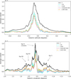 |
Fig. 4 Latitudinal (top) and longitudinal (bottom) profiles of the X64 cleaned map. The profiles have a width of 0.5 degrees, and the different lines correspond to the different components subtracted from the raw 6.4 keV XMM-Newton map. |
X64 band modelling.
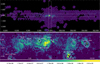 |
Fig. 5 X64 cleaned full map and zoomed-in view, averaged over ∼20 years of XMM-Newton observations. Top: X-ray emission across the entire X64 cleaned map representing the reflection. The white rectangular regions indicate the areas used for profile extraction. Bottom: zoomed-in view of the central degrees of the Galaxy, where the reflected emission is concentrated. Bright sources masked out during the analysis are marked with solid white circles, while known molecular clouds are outlined in dashed white. The position of Sgr A* is denoted by an X. |
4.2 The clean fluorescent map
We present the full XMM-Newton mosaic of the X64 map cleaned for contributions of other components (model C-X67X50) in the top panel of Fig. 5 along with the regions used for profile extraction. We assumed that this map represents a reflected emission coming from dense gas irradiated by X-rays. We note here that this mosaic corresponds to the integrated fluorescent emission over a time period of ∼20 years, with observations in the GC and CMZ being deeper and spanning a longer time period than those of the inner GP where the observations are generally shallower (∼20 ks) and span a time period of four years. Moreover, different parts of the map were observed at different times. We observe that the reflection emission is concentrated in the central degrees of the GC along the CMZ. We show a zoomed-in view of the central ∼2 × 1 degrees in the bottom panel of Fig. 5. In this panel, bright sources masked out during the fitting process and the profile extraction are indicated by solid white circles. Known molecular cloud positions are outlined with dashed white regions, while the location of Sgr A* is marked by an X. All indicated regions show 6.4 keV emission with particular intensity at the Sgr A molecular complex.
A valuable test to investigate how the cleaned X64 map correlates with reflected emission from molecular clouds is to compare its distribution along the CMZ with tracers of molecular gas. For this purpose, we used contours from two surveys that outline molecular gas emission in the GC. Specifically, we used the Herschel SPIRE 250 μm map from the Hi-GAL survey Key Project (Molinari et al. 2010, 2011), which traces a continuous chain of cold and dense clumps, and the N2H+molecular gas emission map from the Mopra survey of the CMZ (Jones et al. 2012). In Fig. 6, we overlay contours from Molinari et al. (2011) and Jones et al. (2012) on the cleaned X64 map, shown in the top and bottom panels, respectively. This comparison reveals a strong correlation with the distribution of cold and dense clumps as well as the molecular gas, suggesting that this emission indeed arises from X-rays reflected by cold gas in molecular clouds illuminated by past X-ray radiation. Perfect agreement between the distribution of cold gas and the reflected X-ray emission is not expected due to the uneven illumination of the clouds and the different observation times by XMM-Newton.
In Fig. 7, we show the fraction of the original (raw) 6.4 keV map that remains after the removal of stars and continuum, plausibly attributed to clean fluorescent emission. We notice that at the position of the most prominent fluorescent features, more than 80% of the raw emission (yellow features) could be attributed to fluorescent emission from molecular gas. Negative regions (shown in black) are present, but of significantly smaller amplitude comparable to the noise level, while areas of the map that do not show reflection remain close to zero (shown in blue). Using the fiducial model, we estimate the non-reflection contribution to the 6.4 keV band, within a central elliptical region consistent to the CMZ (Fig. 3), to a median value of 65%. For regions outside the CMZ the ‘clean reflection’ component approaches zero as is also evident by the latitudinal and longitudinal profiles (Fig. 4). The contribution of the non-reflection component to the CMZ region is significant, and should be considered in future analyses that take into account the pure reflection emission. In addition, the cleaned map can also be used to set upper limits on the 6.4 keV flux from unilluminated molecular complexes, which is crucial for understanding the low-energy cosmic ray ionisation rate and other steady sources of reflection-like emission.
In this work, we filtered out the contribution of the diffuse component that affects the 6.4 keV band while also correlating with the projected mass distribution. As a key point for future studies, we emphasise that the cleaned X64 map serves as a proxy for the time-averaged reflection emission, which is closely linked to the constant illumination of molecular gas in the CMZ. This illumination could be driven by Sgr A*, cosmic rays, or a multitude of bright X-ray sources in the GC region, each predicting different correlations with molecular gas density. For example, single sources (e.g. Sgr A* or X-ray binaries) would show a distance-dependent trend, cosmic ray models might correlate with gamma-ray emission morphologies, and in the case of multiple X-ray sources, we expect a mix of uniform illumination and a centrally peaked contribution from the NSC.
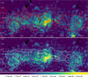 |
Fig. 6 X64 cleaned map with overlaid contours of the cold and dense molecular gas in the CMZ. Top: Herschel SPIRE 250 μm emission contours (Molinari et al. 2011). Bottom: N2H+ molecular emission contours (Jones et al. 2012). |
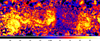 |
Fig. 7 Fraction of the flux in the X64 band that remains after the best-fitting contributions to this band from stars and continuum have been removed. The remaining flux can plausibly be attributed to the fluorescent emission from molecular gas. |
5 Conclusions
In this work, we utilised mosaics of all available XMM-Newton observations of the GC and inner disc, along with SMD models of our Galaxy, to decompose the 6.4 keV line emission into truly reflected emission and contributions from other physical components. Using the spatial correlations of the continuum (X50), 6.7 keV (X67), and 6.4 keV (X64) bands, together with SMD maps, we derived a clean fluorescent X64 map. Key findings include:
For the 6.30−6.50 keV band (X64), a linear combination of the NSC+NSD and bar+disc maps effectively accounts for much of the diffuse emission that is traced by the distribution of stars. This reveals that outside the CMZ region, most of the 6.4 keV emission can be attributed to unresolved point sources;
A linear combination of the X67 and X50 maps produces even cleaner maps (in terms of the residual noise in the X64 map). This, on the one hand, confirms that the diffuse continuum emission correlates strongly with the distribution of stars (i.e. Revnivtsev et al. 2007), similar to the NSD and bar components. In addition, using these maps reduces the residuals associated with the brightest compact sources;
Masking only the bright sources before fitting the maps is insufficient to avoid negative residuals in the final cleaned maps, as the high density of sources in the GC region likely breaks the assumption that physically unrelated signals are spatially uncorrelated, which is essential for using our method. Applying an entire elliptical mask to exclude bright emission in the GC yields optimal results with minimal or no negative residuals, as demonstrated in the Galactic longitudinal and latitudinal profiles;
Our fiducial clean X64 map reveals that the truly diffuse observed emission is confined to the CMZ region;
The cleaned map shows a strong correlation with the distribution of molecular gas and the dense and cold gas in the GC. This component likely represents X-rays reflected by cold gas in molecular clouds illuminated by X-rays.
Given that the residual 6.4 keV emission map we derived closely aligns with the distribution of molecular and cold, dense gas along the CMZ, we argue that this map offers the best estimate for the X-ray reflection signal (observed with XMM-Newton over the last two decades). Furthermore, we estimate that approximately 65% of the ridge emission contributes to the observed 6.4 keV emission in the CMZ. This contribution should be taken into account in future studies, including polarisation analyses of the reflected X-ray continuum from molecular clouds and statistical examinations of reflection surface brightness fluctuations.
Data availability
The cleaned map presented in Fig. 5 is available at the CDS via anonymous ftp to cdsarc.cds.unistra.fr (130.79.128.5) or via https://cdsarc.cds.unistra.fr/viz-bin/cat/J/A+A/698/A313.
Acknowledgements
KA acknowledges support from Chandra grants GO3-24033B, GO0-21010X, and TM9-20001X, and JWST grant JWST-GO-01905.002-A. IK acknowledges support by the COMPLEX project from the European Research Council (ERC) under the European Union’s Horizon 2020 research and innovation program grant agreement ERC-2019-AdG 882679. MCS acknowledges financial support from the European Research Council under the ERC Starting Grant “GalFlow” (grant 101116226) and from Fondazione Cariplo under the grant ERC attrattività no. 2023-3014. GP acknowledges support from the European Research Council (ERC) under the European Union’s Horizon 2020 research and innovation program HotMilk (grant agreement No. 865637), support from Bando per il Finanziamento della Ricerca Fondamentale 2022 dell’Istituto Nazionale di Astrofisica (INAF): GO Large program and from the Framework per l’Attrazione e il Rafforzamento delle Eccellenze (FARE) per la ricerca in Italia (R20L5S39T9). We also made use of NASA’s Astrophysics Data System Bibliographic Services.
Appendix A Recent XMM-Newton observations
XMM-Newton observations.
Appendix B Limitations of the bright source masking strategy
In this section we present the results obtained when masking only the bright sources. We also explain why this strategy does not perform as well as masking in addition, the entire central region affected by reflection using an elliptical mask. The latter is the approach adopted in our main analysis (Sect. 4.1; Fig. 3).
The cleaned map (Fig. B.1) using only the bright source mask shows significant negative residuals when minimising the variance across the entire map – particularly in the GC near Sgr A* and around bright sources. This likely happens since both the peak of the reflected emission and the thermal emission are concentrated in the GC. Hence, some of the reflected emission is removed. This is further reflected in the Galactic longitudinal profiles. When using the bright source mask (Fig. B.2), all models show significant negative residuals particularly close to the GC. When comparing these results to those obtained with elliptical masking (Figs. 3 and 4), the improved performance of the adopted method, with almost no negative residuals, becomes evident.
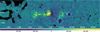 |
Fig. B.1 Example of the cleaned X64 band maps (X64 minus C-X67-X50) when masking only for bright sources. The mask is shown with the cyan circles. Significant negative residuals remain at the GC near Sgr A* and near the bight sources. |
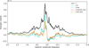 |
Fig. B.2 Longitudinal profiles of the X64 cleaned map when masking only for bright sources. Significant negative residuals remain, particularly at the GC near Sgr A*. |
References
- Anastasopoulou, K., Ponti, G., Sormani, M. C., et al. 2023, A&A, 671, A55 [NASA ADS] [CrossRef] [EDP Sciences] [Google Scholar]
- Bally, J., Stark, A. A., Wilson, R. W., & Henkel, C., 1988, ApJ, 324, 223 [Google Scholar]
- Barret, D., Olive, J. F., Boirin, L., et al. 2000, ApJ, 533, 329 [Google Scholar]
- Bland-Hawthorn, J., & Gerhard, O., 2016, ARA&A, 54, 529 [Google Scholar]
- Bykov, A. M., 2002, A&A, 390, 327 [NASA ADS] [CrossRef] [EDP Sciences] [Google Scholar]
- Capelli, R., Warwick, R. S., Porquet, D., Gillessen, S., & Predehl, P., 2011, A&A, 530, A38 [NASA ADS] [CrossRef] [EDP Sciences] [Google Scholar]
- Capelli, R., Warwick, R. S., Porquet, D., Gillessen, S., & Predehl, P., 2012, A&A, 545, A35 [NASA ADS] [CrossRef] [EDP Sciences] [Google Scholar]
- Chatzopoulos, S., Fritz, T. K., Gerhard, O., et al. 2015, MNRAS, 447, 948 [Google Scholar]
- Chernyshov, D. O., Ko, C. M., Krivonos, R. A., Dogiel, V. A., & Cheng, K. S., 2018, ApJ, 863, 85 [NASA ADS] [CrossRef] [Google Scholar]
- Chuard, D., Terrier, R., Goldwurm, A., et al. 2018, A&A, 610, A34 [NASA ADS] [CrossRef] [EDP Sciences] [Google Scholar]
- Churazov, E., Khabibullin, I., Ponti, G., & Sunyaev, R., 2017a, MNRAS, 468, 165 [Google Scholar]
- Churazov, E., Khabibullin, I., Sunyaev, R., & Ponti, G., 2017b, MNRAS, 465, 45 [Google Scholar]
- Clavel, M., Terrier, R., Goldwurm, A., et al. 2013, A&A, 558, A32 [NASA ADS] [CrossRef] [EDP Sciences] [Google Scholar]
- Clavel, M., Soldi, S., Terrier, R., et al. 2014, MNRAS, 443, L129 [NASA ADS] [CrossRef] [Google Scholar]
- Cooke, B. A., Griffiths, R. E., & Pounds, K. A., 1969, Nature, 224, 134 [NASA ADS] [CrossRef] [Google Scholar]
- Do, T., Kerzendorf, W., Konopacky, Q., et al. 2018, ApJ, 855, L5 [Google Scholar]
- Dogiel, V., Cheng, K.-S., Chernyshov, D., et al. 2009, PASJ, 61, 901 [NASA ADS] [CrossRef] [Google Scholar]
- Feldmeier-Krause, A., Kerzendorf, W., Neumayer, N., et al. 2017, MNRAS, 464, 194 [Google Scholar]
- Fritz, T. K., Patrick, L. R., Feldmeier-Krause, A., et al. 2021, A&A, 649, A83 [NASA ADS] [CrossRef] [EDP Sciences] [Google Scholar]
- GRAVITY Collaboration (Abuter, R., et al.) 2019, A&A, 625, L10 [NASA ADS] [CrossRef] [EDP Sciences] [Google Scholar]
- Heard, V., & Warwick, R. S., 2013, MNRAS, 428, 3462 [NASA ADS] [CrossRef] [Google Scholar]
- Inui, T., Koyama, K., Matsumoto, H., & Tsuru, T. G., 2009, PASJ, 61, S241 [NASA ADS] [CrossRef] [Google Scholar]
- Jin, C., Ponti, G., Haberl, F., & Smith, R., 2017, MNRAS, 468, 2532 [NASA ADS] [CrossRef] [Google Scholar]
- Jin, C., Ponti, G., Haberl, F., Smith, R., & Valencic, L., 2018, MNRAS, 477, 3480 [Google Scholar]
- Jones, P. A., Burton, M. G., Cunningham, M. R., et al. 2012, MNRAS, 419, 2961 [Google Scholar]
- Kallman, T., & White, N. E., 1989, ApJ, 341, 955 [Google Scholar]
- Khabibullin, I., Churazov, E., & Sunyaev, R., 2022, MNRAS, 509, 6068 [Google Scholar]
- Koyama, K., 2018, PASJ, 70, R1 [Google Scholar]
- Koyama, K., Makishima, K., Tanaka, Y., & Tsunemi, H., 1986, PASJ, 38, 121 [NASA ADS] [Google Scholar]
- Koyama, K., Awaki, H., Kunieda, H., Takano, S., & Tawara, Y., 1989, Nature, 339, 603 [NASA ADS] [CrossRef] [Google Scholar]
- Koyama, K., Maeda, Y., Sonobe, T., et al. 1996, PASJ, 48, 249 [Google Scholar]
- Koyama, K., Inui, T., Hyodo, Y., et al. 2007, PASJ, 59, 221 [Google Scholar]
- Krivonos, R., Revnivtsev, M., Churazov, E., et al. 2007, A&A, 463, 957 [NASA ADS] [CrossRef] [EDP Sciences] [Google Scholar]
- Krivonos, R., Clavel, M., Hong, J., et al. 2017, MNRAS, 468, 2822 [CrossRef] [Google Scholar]
- Krivonos, R., Shtykovskaya, E., & Sazonov, S., 2025, J. High Energy Astrophys., 45, 96 [Google Scholar]
- Kuznetsova, E., Krivonos, R., Clavel, M., et al. 2019, MNRAS, 484, 1627 [CrossRef] [Google Scholar]
- Kuznetsova, E., Krivonos, R., Lutovinov, A., & Clavel, M., 2022, MNRAS, 509, 1605 [Google Scholar]
- Launhardt, R., Zylka, R., & Mezger, P. G., 2002, A&A, 384, 112 [NASA ADS] [CrossRef] [EDP Sciences] [Google Scholar]
- Marin, F., Churazov, E., Khabibullin, I., et al. 2023, Nature, 7968, 41 [Google Scholar]
- Molinari, S., Swinyard, B., Bally, J., et al. 2010, A&A, 518, L100 [NASA ADS] [CrossRef] [EDP Sciences] [Google Scholar]
- Molinari, S., Bally, J., Noriega-Crespo, A., et al. 2011, ApJ, 735, L33 [Google Scholar]
- Muno, M. P., Baganoff, F. K., Bautz, M. W., et al. 2004, ApJ, 613, 326 [NASA ADS] [CrossRef] [Google Scholar]
- Muno, M. P., Baganoff, F. K., Brandt, W. N., Park, S., & Morris, M. R., 2007, ApJ, 656, L69 [NASA ADS] [CrossRef] [Google Scholar]
- Murakami, H., Koyama, K., & Maeda, Y., 2001, ApJ, 558, 687 [Google Scholar]
- Neumayer, N., Seth, A., & Böker, T., 2020, A&A Rev., 28, 4 [NASA ADS] [CrossRef] [Google Scholar]
- Nishiyama, S., Yasui, K., Nagata, T., et al. 2013, ApJ, 769, L28 [Google Scholar]
- Park, S., Muno, M. P., Baganoff, F. K., et al. 2004, ApJ, 603, 548 [NASA ADS] [CrossRef] [Google Scholar]
- Planck Collaboration XXII., 2016, A&A, 594, A22 [NASA ADS] [CrossRef] [EDP Sciences] [Google Scholar]
- Ponti, G., Terrier, R., Goldwurm, A., Belanger, G., & Trap, G., 2010, ApJ, 714, 732 [NASA ADS] [CrossRef] [Google Scholar]
- Ponti, G., Morris, M. R., Terrier, R., & Goldwurm, A., 2013, in Cosmic Rays in Star-Forming Environments, eds. D. F. Torres & O. Reimer, Astrophysics and Space Science Proceedings, 34, 331 [NASA ADS] [CrossRef] [Google Scholar]
- Ponti, G., Morris, M. R., Terrier, R., et al. 2015, MNRAS, 453, 172 [Google Scholar]
- Ponti, G., Hofmann, F., Churazov, E., et al. 2019, Nature, 567, 347 [Google Scholar]
- Portail, M., Gerhard, O., Wegg, C., & Ness, M., 2017, MNRAS, 465, 1621 [NASA ADS] [CrossRef] [Google Scholar]
- Revnivtsev, M., Molkov, S., & Sazonov, S., 2006a, MNRAS, 373, L11 [Google Scholar]
- Revnivtsev, M., Sazonov, S., Gilfanov, M., Churazov, E., & Sunyaev, R. 2006b, A&A, 452, 169 [NASA ADS] [CrossRef] [EDP Sciences] [Google Scholar]
- Revnivtsev, M., Vikhlinin, A., & Sazonov, S., 2007, A&A, 473, 857 [NASA ADS] [CrossRef] [EDP Sciences] [Google Scholar]
- Revnivtsev, M., Sazonov, S., Churazov, E., et al. 2009, Nature, 458, 1142 [Google Scholar]
- Ryu, S. G., Nobukawa, M., Nakashima, S., et al. 2013, PASJ, 65, 33 [Google Scholar]
- Schödel, R., Feldmeier, A., Kunneriath, D., et al. 2014, A&A, 566, A47 [Google Scholar]
- Schultheis, M., Fritz, T. K., Nandakumar, G., et al. 2021, A&A, 650, A191 [NASA ADS] [CrossRef] [EDP Sciences] [Google Scholar]
- Sormani, M. C., Gerhard, O., Portail, M., Vasiliev, E., & Clarke, J., 2022a, MNRAS, 514, L1 [Google Scholar]
- Sormani, M. C., Sanders, J. L., Fritz, T. K., et al. 2022b, MNRAS, 512, 1857 [Google Scholar]
- Stel, G., Ponti, G., Haardt, F., & Sormani, M., 2025, A&A, 695, A52 [NASA ADS] [CrossRef] [EDP Sciences] [Google Scholar]
- Sunyaev, R. A., Markevitch, M., & Pavlinsky, M., 1993, ApJ, 407, 606 [Google Scholar]
- Terrier, R., Ponti, G., Bélanger, G., et al. 2010, ApJ, 719, 143 [Google Scholar]
- Uchiyama, H., Nobukawa, M., Tsuru, T., Koyama, K., & Matsumoto, H., 2011, PASJ, 63, S903 [NASA ADS] [CrossRef] [Google Scholar]
- Valinia, A., Tatischeff, V., Arnaud, K., Ebisawa, K., & Ramaty, R., 2000, ApJ, 543, 733 [Google Scholar]
- Wang, Q. D., Gotthelf, E. V., & Lang, C. C., 2002, Nature, 415, 148 [NASA ADS] [CrossRef] [Google Scholar]
- Wang, Q. D., Dong, H., & Lang, C., 2006, MNRAS, 371, 38 [Google Scholar]
- Worrall, D. M., Marshall, F. E., Boldt, E. A., & Swank, J. H., 1982, ApJ, 255, 111 [Google Scholar]
- Xu, X.-j., Wang, Q. D., & Li, X.-D. 2016, ApJ, 818, 136 [NASA ADS] [CrossRef] [Google Scholar]
- Yamauchi, S., & Koyama, K., 1993, ApJ, 404, 620 [Google Scholar]
- Yamauchi, S., Nobukawa, K. K., Nobukawa, M., Uchiyama, H., & Koyama, K., 2016, PASJ, 68, 59 [NASA ADS] [CrossRef] [Google Scholar]
- Yuasa, T., Makishima, K., & Nakazawa, K., 2012, ApJ, 753, 129 [NASA ADS] [CrossRef] [Google Scholar]
- Yusef-Zadeh, F., Law, C., & Wardle, M., 2002, ApJ, 568, L121 [NASA ADS] [CrossRef] [Google Scholar]
- Yusef-Zadeh, F., Muno, M., Wardle, M., & Lis, D. C., 2007, ApJ, 656, 847 [Google Scholar]
- Zhu, Z., Li, Z., & Morris, M. R., 2018, ApJS, 235, 26 [NASA ADS] [CrossRef] [Google Scholar]
The model by Feldmeier-Krause et al. (2017) estimates a lower total mass for the NSC.
We utilised a distance to the GC of 8.2 kpc (GRAVITY Collaboration 2019), an EPIC pn effective area of 460 cm−2, and a mass surface density of 103 M⊙ pix−1.
All Tables
All Figures
|
Fig. 1 Spectral representation of the three energy bands used in this project. The bands are highlighted by the shaded regions. The representative model spectra (convolved with the XMM-Newton spectra response function) of hot plasma (apec model in XSPEC) and reflection (crefl16 model; Churazov et al. 2017b) are shown as orange and blue lines, respectively. |
| In the text | |
|
Fig. 2 Raw maps used in this study. From top to bottom: the XMM-Newton 6.4 keV (X64), 6.7 keV (X67), the continuum band (X50), and the SMD. The XMM-Newton maps are measured in count per second per pixel (cr/pix), whereas the SMD map represents stellar density in 103 M⊙/pix. The colour bar ranges are selected arbitrarily to emphasise and display morphological differences. The x-axis and y-axis represent the Galactic longitude and latitude, respectively, in degrees. |
| In the text | |
|
Fig. 3 Example of the cleaned X64 band map (X64 minus C-X67-X50). The mask is shown as a dashed ellipse, and solid circles correspond to bright sources. The map is in units of counts per second per pixel. Black regions indicate areas with no exposure, which may result from the removal of point sources, stray-light artefacts, or chip gaps. |
| In the text | |
|
Fig. 4 Latitudinal (top) and longitudinal (bottom) profiles of the X64 cleaned map. The profiles have a width of 0.5 degrees, and the different lines correspond to the different components subtracted from the raw 6.4 keV XMM-Newton map. |
| In the text | |
|
Fig. 5 X64 cleaned full map and zoomed-in view, averaged over ∼20 years of XMM-Newton observations. Top: X-ray emission across the entire X64 cleaned map representing the reflection. The white rectangular regions indicate the areas used for profile extraction. Bottom: zoomed-in view of the central degrees of the Galaxy, where the reflected emission is concentrated. Bright sources masked out during the analysis are marked with solid white circles, while known molecular clouds are outlined in dashed white. The position of Sgr A* is denoted by an X. |
| In the text | |
|
Fig. 6 X64 cleaned map with overlaid contours of the cold and dense molecular gas in the CMZ. Top: Herschel SPIRE 250 μm emission contours (Molinari et al. 2011). Bottom: N2H+ molecular emission contours (Jones et al. 2012). |
| In the text | |
|
Fig. 7 Fraction of the flux in the X64 band that remains after the best-fitting contributions to this band from stars and continuum have been removed. The remaining flux can plausibly be attributed to the fluorescent emission from molecular gas. |
| In the text | |
|
Fig. B.1 Example of the cleaned X64 band maps (X64 minus C-X67-X50) when masking only for bright sources. The mask is shown with the cyan circles. Significant negative residuals remain at the GC near Sgr A* and near the bight sources. |
| In the text | |
|
Fig. B.2 Longitudinal profiles of the X64 cleaned map when masking only for bright sources. Significant negative residuals remain, particularly at the GC near Sgr A*. |
| In the text | |
Current usage metrics show cumulative count of Article Views (full-text article views including HTML views, PDF and ePub downloads, according to the available data) and Abstracts Views on Vision4Press platform.
Data correspond to usage on the plateform after 2015. The current usage metrics is available 48-96 hours after online publication and is updated daily on week days.
Initial download of the metrics may take a while.