| Issue |
A&A
Volume 689, September 2024
|
|
|---|---|---|
| Article Number | A278 | |
| Number of page(s) | 12 | |
| Section | Galactic structure, stellar clusters and populations | |
| DOI | https://doi.org/10.1051/0004-6361/202449419 | |
| Published online | 19 September 2024 | |
Study of X-ray emission from the S147 nebula by SRG/eROSITA: Supernova-in-the-cavity scenario
1
Universitäts-Sternwarte, Fakultät für Physik, Ludwig-Maximilians-Universität München, Scheinerstr.1, 81679 München, Germany
2
Space Research Institute (IKI), Profsoyuznaya 84/32, Moscow 117997, Russia
3
Max Planck Institute for Astrophysics, Karl-Schwarzschild-Str. 1, 85741 Garching, Germany
4
Institute of Astronomy, Russian Academy of Sciences, 48 Pyatnitskaya str., Moscow 119017, Russia
5
Ioffe Institute, Politekhnicheskaya st. 26, Saint Petersburg 194021, Russia
6
Institute for Advanced Study, Einstein Drive, Princeton, New Jersey 08540, USA
7
NRC ‘Kurchatov Institute’, acad. Kurchatov Square 1, Moscow 123182, Russia
8
Institute of Applied Physics of the Russian Academy of Sciences, 46 Ul’yanov str., Nizhny Novgorod 603950, Russia
9
Institut für Astronomie und Astrophysik Tübingen, Universität Tübingen, Sand 1, D-72076 Tübingen, Germany
10
Max-Planck Institut für extraterrestrische Physik, Giessenbachstraße, 85748 Garching, Germany
11
Max-Planck Institut für Radioastronomie, Auf dem Hügel 69, 53121 Bonn, Germany
12
Dr. Karl Remeis Observatory, Erlangen Centre for Astroparticle Physics, Friedrich-Alexander-Universität Erlangen-Nürnberg, Sternwartstraße 7, 96049 Bamberg, Germany
Received:
30
January
2024
Accepted:
8
May
2024
Abstract
The Simeis 147 nebula (S147) is particularly well known for a spectacular net of Hα-emitting filaments. It is often considered one of the largest and oldest (∼105 yr) cataloged supernova remnants in the Milky Way, although the kinematics of the pulsar PSR J0538+2817 suggests that this supernova remnant might be a factor of three younger. The former case is considered in a companion paper, while here we pursue the latter. Both studies are based on the data of SRG/eROSITA All-Sky Survey observations. Here, we confront the inferred properties of the X-ray emitting gas data with the scenario of a supernova explosion in a low-density cavity, such as a wind-blown-bubble. This scenario assumes that a ∼20 M⊙ progenitor star has had a low velocity with respect to the ambient interstellar medium, and so stayed close to the center of a dense shell created during its main-sequence evolution till the moment of the core-collapse explosion. The ejecta first propagate through the low-density cavity until they collide with the dense shell, and only then does the reverse shock go deeper into the ejecta and power the observed X-ray emission of the nebula. The part of the remnant inside the dense shell remains non-radiative till this point, plausibly in a state with Te < Ti and nonequilibrium ionization. On the contrary, the forward shock becomes radiative immediately after entering the dense shell, and, being subject to instabilities, gives the nebula its characteristic “foamy” appearance in Hα and radio emission.
Key words: ISM: supernova remnants
Corresponding author; This email address is being protected from spambots. You need JavaScript enabled to view it. .
© The Authors 2024
 Open Access article, published by EDP Sciences, under the terms of the Creative Commons Attribution License (https://creativecommons.org/licenses/by/4.0), which permits unrestricted use, distribution, and reproduction in any medium, provided the original work is properly cited.
This article is published in open access under the Subscribe to Open model.
Open Access funding provided by Max Planck Society.
1. Introduction
The Simeis 147 nebula (hereafter S147) discovered by G. A. Shajn (Gaze & Shajn 1952) is famous due to its spectacular filamentary appearance in Hα line emission (Lozinskaia 1976). Nonthermal radio (Denoyer 1974; Sofue et al. 1980; Fuerst & Reich 1986; Xiao et al. 2008; Khabibullin et al. 2024) and gamma-ray emission (Katsuta et al. 2012; Suzuki et al. 2022) has been detected from it, indicating that it is most likely a remnant of a supernova (SN) explosion (SNR G180.0-01.7), possibly interacting with a molecular cloud at one of its boundaries. A radio and X-ray pulsar was discovered within the extent of the nebula (Anderson et al. 1996; Kramer et al. 2003), for which the measured proper motion is directed away from the geometrical center of the nebula (Romani & Ng 2003), indicating that S147 might indeed be powered by a core-collapse SN explosion that took place ∼30 000 yr ago (Gvaramadze 2006; Ng et al. 2007).
The size of S147, however, is indicative of a much older explosion: ∼150 000 yr old, if canonical values of the explosion energy and the density of the surrounding medium are assumed (e.g. Silk & Wallerstein 1973). This “age dilemma” (Reich et al. 2003; Romani & Ng 2003) can be reconciled if a scenario of an explosion in the wind-blown cavity is invoked, allowing the size of the object to be determined by winds before the explosion (Reich et al. 2003; Gvaramadze 2006). Although such a picture might be relevant for the bulk of the massive stars (e.g. Dwarkadas 2023) the relative motion of the star through the surrounding interstellar medium (ISM) apparently makes in-cavity explosions rare.
The evolution of the SN blast wave inside a wind-blown cavity differs substantially from the self-similar solution of a point explosion in a uniform medium. It is characterized by a prolonged phase of free expansion (until ejecta hit the walls of the cavity) and a rapid onset of the radiative phase of the forward shock launched into the dense shell (Chevalier & Liang 1989; Tenorio-Tagle et al. 1991).
In the same time, after the passage of the reverse shock through the SN ejecta, the cavity should be filled with the hot X-ray-emitting gas, bearing traces of enrichment by explosive nucleosynthesis products. Given the large size of S147, this emission is expected to be rather faint and difficult to observe, with focusing X-ray telescopes like Chandra, XMM-Newton, or Suzaku having relatively small fields of view. In the course of the all-sky survey (Predehl et al. 2021; Sunyaev et al. 2021), a map of the full extent of the nebula was obtained by SRG/eROSITA, resulting in the first clear detection of soft thermal X-ray emission from S147, with most of the flux coming at energies below ∼1 keV, as we describe in Michailidis et al. (2024) (hereafter Paper I).
In this paper, we consider key spatial and spectral properties of the newly detected X-ray emission from S147 in relation to the physical scenario of a SN explosion in an interstellar cavity created by the progenitor star during its main-sequence (MS) phase. A canonical SNR in a uniform medium scenario is considered and confronted with X-ray and multiwavelength data on S147 in Paper I.
The paper is structured as follows: we give basic information on X-ray observations in Section 2 and outline morphological and spectral properties of the X-ray emission in Section 3. The model of a SN explosion in a wind-blown bubble (WBB), capable of explaining the major properties of the object, is presented in Section 4 and discussed in Section 5. Conclusions are summarized in Section 6
2. Observations
The X-ray data used in this paper are identical to those used and described in Paper I. Namely, they are based on observations of SRG/eROSITA in all four consecutive all-sky surveys (Sunyaev et al. 2021). For imaging analysis, the data of all seven eROSITA telescope modules (TMs) were used, while the data of two TMs without an on-chip optical blocking filter were excluded from the spectral analysis due to their different spectral response function and susceptibility to optical light leak contamination at low energies (e.g. Predehl et al. 2021).
3. X-ray emission
A comprehensive description of various properties of X-ray emission detected in the direction of the S147 nebula is presented in Paper I; here, we focus on key features that might support the physical scenario that we put forward in Section 4.
3.1. Broadband X-ray morphology
Figure 1 shows the surface brightness of the X-ray emission in the 0.5–1 keV band from a 3.7° × 3.7° patch (in Galactic coordinates) covering the full extent of S147. The image was produced by masking the detected point and mildly extended sources and smoothing with a Gaussian kernel with σ = 1′. The exact procedure is identical to the one used in previous works on the newly discovered X-ray supernova remnants (SNRs) (Churazov et al. 2021; Khabibullin et al. 2023) and is described in Paper I. The image is centered close to the geometrical center of the Hα and radio emission, at (l, b)≈(180.32° , − 1.65° ) (e.g. Kramer et al. 2003), and the position of the pulsar PSR is marked with a cross (the point-like emission of the pulsar itself has been masked). The ratio of the X-ray emission from the SNR to the unrelated background and foreground emission is maximized in this band (the latter was estimated from adjacent sky regions outside the extent of the nebula). At lower and higher energies, the S147 emission falls below the background level, making it barely visible in the 2D image, but still detectable in the background-subtracted source spectrum.
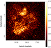 |
Fig. 1. Broadband (0.5–1.0 keV) (particle) background-subtracted, exposure-corrected X-ray image (linear scale) obtained by SRG/eROSITA in the S147 direction (3.7° × 3.7° in Galactic coordinates) after masking of point and mildly extended sources and smoothing with a Gaussian kernel with σ = 1′. This band maximizes the source-to-background ratio for the SNR emission. The cross marks the position of the pulsar PSR. |
The morphology of the X-ray emission is drastically different from the filamentary and more circular morphology of the Hα and radio emission, as is illustrated in Figure 2 (top panel), which combines the same SRG/eROSITA X-ray image (blue) with the Hα image (green) from the IGAPS survey (Greimel et al. 2021) and radio image at 1.4 GHz (red) from the CGPS survey (Taylor et al. 2003). Both latter images were convoluted with a median top-hat filter (r = 40″) suppressing numerous point sources but leaving diffuse and filamentary emission mostly unaffected.
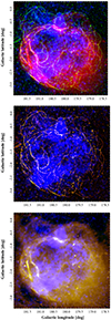 |
Fig. 2. Multiwavelength view of S147 (in Galactic coordinates). Top: combined map of the radio (CGPS data at 1.4 GHz, red), wavelet-decomposed (in order to emphasize filamentary structure) Hα (IGAPS data, green), and broadband X-ray (0.5–1.1 keV, SRG/eROSITA data, blue) emission. The white cross marks the position of PSR J0538+2817. Middle: the intensity-saturated X-ray image is shown in blue on top of the wavelet-decomposed Hα image, demonstrating that X-ray emission is confined by the Hα-emitting shell. Bottom: same as the middle panel but with the 1.4 GHz radio emission as a background. |
One can see that the X-ray emission is not clearly structured and contains regions of brighter and fainter (by a factor of a few compared to the mean one) emission, which are ∼1/3 − 1/10 of the full size of the nebula (R ∼ 100′) and appear in the form of “blobs” and “depressions” on top of the smooth background emission. No signatures of the global edge-brightening or central peak are visible.
Comparisons with the Hα and radio images indicate that some of the bright X-ray regions lie close to the brightest optical and radio filaments (as is exemplified by the bright region and filaments to the Galactic north of the nebula’s center at l, b = 180.25° , − 0.75°), while other bright X-ray regions (like the one to the Galactic south of the center at l, b = 180.5° , − 2.5°) lack prominent counterparts. On the other hand, the largest cavity in X-ray emission, at l, b = 180.75° , − 1.75°, also coincides with the region of fainter optical and radio emission. No signatures of filamentary X-ray emission are visible.
The X-ray emission appears to be well confined by the optical and radio boundaries. The latter point is even more clearly illustrated by the images in the middle and bottom panels of Figure 2, which show intensity-saturated broadband X-ray image (blue) on top of wavelet decomposed Hα (top panel, highlighting the filamentary optical emission). and radio emission. One can see that X-ray emission reaches the boundaries of the optical and radio emission in the eastern part of the nebula, while it ends slightly short of it on the western side (appearing more diffuse in the radio and structured on smaller scales in the optical bands). Comparisons with the dust and interstellar absorption maps for this region show no correlations with X-ray morphology on these scales, indicating that the observed variations are intrinsic to the source itself (cf. also a dedicated discussion in Paper I).
3.2. Narrow-band imaging
Given the inhomogeneous appearance of the X-ray emission from S147 and its complex connection to the emission at other wavelengths, we checked for possible correlated spatial variations in its spectral shape by comparing maps accumulated in narrow energy bands centered on the brightest emission lines in the thermal plasma at kT = 0.1 − 0.3 keV: O VII, O VIII, and Ne IX (as is shown for the entire SNR’s spectrum in Figure 3). Namely, Figure 4 shows images in the 0.44-0.62, 0.62–0.8, and 0.8–1.1 keV bands, as well as their RGB combination.
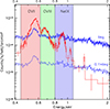 |
Fig. 3. X-ray spectrum of the whole remnant (red data points) after subtraction of the background signal (blue data points) estimated from an adjacent sky region. Also shown is the level of 10% of the background emission, which aims to show that above 1.5 keV the SN signal amounts to a few % of the background level, making conclusions regarding its spectral shape at these energies strongly background-sensitive. The three bands containing the brightest emission lines are shown in red (O VII), green (O VII), and blue (Ne IX), and are used for RGB composite images. |
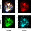 |
Fig. 4. RGB-composite (top left) and individual narrow-band X-ray images covering the 0.44–1.1 keV band. The red, green, and cyan (instead of blue, for better visibility) images correspond to the 0.44–0.62, 0.62–0.8, and 0.8–1.1 keV bands, respectively. These bands encompass the three brightest X-ray emission lines in the spectrum of S147: O VII, O VIII, and Ne IX. |
Although moderate “color” variations are clearly visible in the RGB image, all three images share a rather similar morphology. Emission in the O VII appears most diffuse, while O VIII appears to be more filament-structured, and Ne IX appears somewhat edge-brightened. These observations justify the consideration of the single spectrum of the full nebula as a proxy for the physical conditions of the X-ray-emitting material. Analysis of the spectra extracted from the individual regions is presented in Paper I and confirms the validity of this assumption.
3.3. X-ray spectra
In this section, we consider the most basic characteristics of the entire SNR’s X-ray spectrum. The spectrum shown in Fig. 5 features three very prominent lines (O VII, O VIII, and Ne IX) below 1 keV and weaker lines at higher energies, of which the line of Mg XI is the most significant.
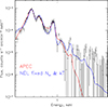 |
Fig. 5. X-ray spectrum of the entire S147 SNR. The red line shows the best-fitting APEC model (single-temperature, CIE, solar abundance of metals). This model requires a very large absorbing column density, overpredicts the flux near 0.8 keV (where a significant contribution of Fe XVII line at 826 eV is expected), and underpredicts the Mg XI line flux unless its abundance (relative to oxygen) is very high. For comparison, the blue line shows the NEI model with parameters fixed at physically motivated values. Although formally the value of χ2 is higher than for the APEC model, the lower value of NH and the ability of the model to better describe regions near Fe XVII and Mg XI lines make this model an appealing interpretation of the S147 spectrum (see text for details). |
A starting minimalist’s assumption is that for an old SNR, the X-ray emission might be well described by the thermal emission of plasma in collisional ionization equilibrium (CIE). To this end, an absorbed APEC model with a fixed (=solar) abundance of heavy elements can be used. However, this model fails in two aspects: it requires a large absorbing column density (NH ∼ 0.6 × 1022 cm−2, which is significantly larger than the expected value, (0.2 − 0.4)×1022 cm−2), overpredicts the flux near ∼0.8 keV, and underpredicts the flux in the line of Mg XI. This is also reflected in the value of χ2 (366 for 318 d.o.f.; see Table 1). In practice, a large value of χ2 is anticipated given the complexity of the remnant. The integrated spectrum might include several spectral components with different temperatures and metallicities. We therefore do not consider the value of χ2 to be a robust quantitative way of ranking complicated models. Instead, we want to demonstrate that for a set of physically motivated parameters, the model can qualitatively reproduce the observed spectrum. For the S147 model outlined in the abstract, another spectral model is better motivated. Due to the large size and low density of the gas in the cavity, the ejecta reheated by the reverse shock some 15 kyr ago can remain hot for a long time and may deviate from the CIE. This can happen even if ejecta are mixed with a moderate amount of gas that was present in the cavity. However, a single nonequilibrium ionization (NEI) model converges to a solution that is not very far from the APEC parameters (large NH and low kT), although with a better χ2. This is clearly driven by the requirement to describe the O VII/O VIII ratio, where statistics is the highest, and less weight is given to other parts of the spectrum. One can further try to push ahead the NEI scenario by fixing the absorbing column density to the expected value of NH ∼ 2.5 × 1021 cm−2 and the electron temperature to a sufficiently high value, such as kT = 1 keV. This model has a higher χ2 value, but it better describes the spectrum near ∼0.8 keV and boosts the flux in the Mg XI line, making this model an appealing interpretation of the S147 spectrum.
Simplest spectral model fits to the spectrum of the entire SNR in the 0.4–3 keV band.
The above analysis was done assuming that the abundance of heavy metals is solar. This assumption can be far from reality if X-ray emission is coming from the ejecta. Since at relatively low temperatures, metals’ contribution dominates the X-ray emission, the absolute abundance measurements are difficult, while the relative abundances are more robust. Since the lines of oxygen dominate in the observed spectrum, it is convenient to express abundances relative to oxygen rather than hydrogen. In the models described below (Section 4.4), the ejecta abundances of C, N, and Fe (relative to O) are ∼30% of the solar values, while the abundances of Ne and Mg vary between between 0.6 and 1.7 (relative to O). Letting the abundance of elements free would make the model much more flexible but less constrained. Since the abundance variations relative to oxygen are not very extreme, we freeze the ratios at the solar values but keep in mind that the line ratios might not be accurately predicted by the model. Another important result of the increased abundance is the difference in the derived emission measure that scales approximately linearly with the abundance (as long as metals dominate the spectrum).
4. The model: A supernova explosion in a wind-blown bubble
The idea that an SN might explode in a wind-blown cavity was first proposed for the SNR N132D in LMC (Hughes 1987). In that particular case, the cavity was invoked to resolve the disparity between the large Sedov expansion age and the much smaller age inferred from oxygen-rich optical filaments. In the case of S147, we face a somewhat similar age puzzle.
4.1. S147 age dilemma
It is highly likely that the pulsar J0538+2817 and SNR S147 have a common origin, which is suggested by the pulsar motion directed from the shell center (Romani & Ng 2003). The pulsar distance inferred from VLBI parallax is 1.3 kpc and the proper motion μ = 57.9 mas yr−1 (Chatterjee et al. 2009). The most recent absorption-based distance estimates for S147 (e.g., Paper I, Kochanek et al. 2024) are consistent with this value. The pulsar offset of 0° .605, combined with the proper motion, implies a pulsar kinematic age of tkin = 37.6 kyr. With an SNR angular radius of Hα filamentary shell of 100′, the physical shell radius is r = 39 pc.
The S147 expansion velocity implied by Hα spectroscopic observations is about 100 km s−1 km s−1 (Lozinskaia 1976). This value is consistent with the LAMOST optical spectroscopic survey in the field of S147, which shows a symmetric velocity distribution of the line-emitting gas in the range of ±100 km s−1 (Ren et al. 2018). Assuming that the SNR expansion takes place in a homogeneous medium with a typical density, one can derive the lower limit for the age by applying the Sedov solution for the point explosion. The inferred SNR age is then texp = 0.4r/v = 150 kyr, which is four times larger than the kinematic age (37.6 kyr). It should be noted that the radiative expansion regime would produce an even larger age. Alternatively, adopting an expansion age of 37.6 kyr and radius of 39 pc, one would expect a shell expansion velocity of v = 0.4r/t = 407 km s−1, which is four times the observed expansion velocity of 100 km s−1.
The disparity between the kinematic and Sedov expansion ages has been recognized by Reich et al. (2003) and Romani & Ng (2003). To resolve the age dilemma, Reich et al. (2003) proposed that S147’s progenitor exploded in a WBB, with a subsequent SNR deceleration after the collision with a boundary of the massive swept-up shell. We consider this scenario to be a likely possibility and explore it in more detail.
4.2. The wind-blown bubble
As an illustration of the WBB conjecture for the S147, we considered the case of a massive SN II progenitor of about 20 M⊙. This case is relevant because it falls in the range of 9–25 M⊙ responsible for neutron star production (Woosley et al. 2002; Heger et al. 2003); besides, the 20 M⊙ mass is high enough to produce an extended WBB for the typical ISM density.
Usually, the WBB radius in a homogeneous ISM is estimated using a well-known analytic solution (Weaver et al. 1977). However, to find a more adequate estimate of the expected radius, one needs to take into account the ISM pressure, which is omitted from this analytic solution. We used a thin shell approximation to solve numerically the equations of mass, momentum, and energy conservation of the Weaver et al. (1977) model with the inclusion of the ISM pressure. The latter is composed of the thermal pressure of the warm ionized medium (WIM) component with nT ≈ 3000 cm−3 K (Cox 2005) and a relativistic pressure of the interstellar magnetic field of B ≈ 3 × 10⁻⁶ G (B2/8π ≈ 3.6 × 10⁻¹³ dyn cm−2), combined with the comparable pressure of cosmic rays. All in all, one expects a total medium pressure of ≈10−12 dyn cm−2.
Major properties of the model bubble for the ISM density of 0.3 cm−3 and three choices of ISM pressure are illustrated by Figure 6 and Table 2. The table contains as input parameters the stellar mass, MS lifetime (Schaller et al. 1992), mass loss rate, wind velocity, ISM pressure, and characteristics at the end of the MS: the bubble radius, bubble density, and the shell’s swept-up mass. The adopted wind parameters correspond to those of a MS O-star with a mass of 20–25 M⊙ (Howarth & Prinja 1989). The MS wind (0.7 M⊙) is thermalized in the termination shock with the radius rt ≈ 3 pc and uniformly fills the cavity volume.
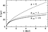 |
Fig. 6. Radius of the wind-driven bubble formed by the 20 M⊙ star wind at the MS. The lines are labeled according to the ISM pressure. The model with zero pressure shows the bubble radius based on the analytic solution (Weaver et al. 1977). |
Parameters of the bubble model.
At the He-burning stage (0.79 Myr), the progenitor becomes a red supergiant (RSG) and loses matter via the slow wind (∼15 km s−1), with a mass loss rate of about 10−6 Myr. Almost all the RSG wind (≈1 M⊙) is expected to be swept up, due to the bubble’s counterpressure, into the dense shell with a radius of ≈1 pc, which is significantly smaller than the bubble’s radius.
4.3. Effect of cloudy interstellar medium
The model of an almost empty WBB in a homogeneous medium is an idealization. The H I 21 cm data (Dickey & Garwood 1989) imply that the mass spectrum of interstellar clouds, both molecular and diffuse atomic, is dN/dm ∝ m−γ, with γ ∼ 2. Therefore, within ∼2 × 10³ M⊙ of ISM swept up by S147, one would expect to find a significant number of parsec-size clouds with a density of 10–100 cm−3.
The key question is whether some of these clouds avoid disruption by the dense bubble shell and end up inside the bubble. A cloud, in order to cross the shell safely, should have a column density of Nc ≈ ncrc, which is significantly larger than the shell column density, Ns = nrb/3 ∼ 1019 cm−2 (for n = 0.3 cm−3 and rb = 30 pc). A typical cloud that meets this requirement might have a radius of ∼1 pc and density of nc = 30 cm−3, in which case Nc ≈ 1020 cm−2, greater than Ns by a factor of ten. Typical column densities of molecular clouds are 1–2 orders of magnitude higher (e.g., Larson 1981;Heyer & Dame 2015). One therefore would expect to find a significant number of parsec-size interstellar clouds engulfed by the bubble. While these clouds do not affect the bubble dynamics, expanding SN ejecta will crush clouds and disperse them into fragments with eventual mixing, thus producing overdensities after their thermalization by the reverse shock.
A cloud with a radius of 1 pc and H density of 30 cm−3 has a mass of ≈3 M⊙. Whether such clouds can survive a complete stripping due to photoevaporation before the bubble shell crossing depends on the cloud mass, m, and ionizing flux, Q/R2, as ṁ ∝ m3/5(Q/R2)1/5 (Bertoldi & McKee 1990). Using the relevant expression from this paper, we find that a cloud with a mass of > 1 M⊙ at a distance of r ≳ 20 pc survives the photoevaporation during the MS lifetime of a 20 M⊙ star, and thus has a chance of finding itself in the bubble.
4.4. Ejecta
To follow the development of the SN explosion within the extended WBB, we exploded the pre-SN model based on a 20 M⊙ progenitor evolved by Woosley et al. (2002) from the MS up to the onset of core collapse. Unfortunately, Woosley et al. (2002) used such a high mass-loss rate that the resultant mass of the corresponding pre-SN was 14.7 M⊙. In turn, we used a moderate mass-loss rate and assumed that the 20 M⊙ progenitor lost ≈0.7 M⊙ in the MS stage and ∼1 M⊙ during the RSG phase. For our problem, therefore, we used a pre-SN model of 18.5 M⊙. To construct the relevant pre-SN model, we modified the original pre-SN model of 14.7 M⊙ by increasing the mass of the hydrogen-rich envelope up to 12.4 M⊙, preserving both the helium core of 6.1 M⊙ and the shape of the profile of density in the hydrogen-rich envelope except for the interface between the helium core and the envelope. The obtained model was exploded with the energy of 1051 erg by a piston at the outer edge of the central collapsing core of 1.46 M⊙. The artificial mixing applied to the pre-SN model mimics the intense 3D turbulent mixing occurring at the (C+O)/He and He/H composition interfaces during the explosion (Utrobin et al. 2017). In addition, radioactive 56Ni with a mass of 0.07 M⊙, typical of type II SNe, was mixed artificially in the velocity space up to nearly 3000 km s−1. Figure 7 shows the profiles of important chemical elements in the freely expanding ejecta. In light of an analysis of the content of these elements, we investigated the pre-SN models of the progenitor masses in the range from 18 M⊙ to 22 M⊙ (Woosley et al. 2002). In particular, we find that the total Mg mass in the ejecta of the 19 M⊙ progenitor is twice as large as that of the 20 M⊙ progenitor.
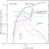 |
Fig. 7. Ejecta structure for the 1B-M20 model. The solid black line shows the enclosed ejecta mass (for a given velocity). The dashed colored lines show which velocities make the largest contribution to the mass of a given element; namely, the quantity 4πr3ρi, where ρi is the mass density of the i-th element, color-coded as in the legend. The solid colored lines show the mass density of the i-th element relative to the mass density of oxygen, normalized by the solar value. |
4.5. Morphology of the Hα emission
There is no doubt that the intricate spaghetti-like structure is a complicated manifestation of the late radiative stage of the SNR, which is liable to different instabilities (Blondin et al. 1998). The forward shock temperature, assuming Te = Ti, is T = 1.36 × 10⁵v72 K. The cooling time in the post-shock gas for the shock with a speed of 100 km s−1 (Lozinskaia 1976) is
 (1)
(1)
where Λ(T)≈10−21 erg s−1 cm3 (Sutherland & Dopita 1993). With tc ≪ t, the forward shock is indeed radiative.
Pikel’ner (1954) proposed that the Hα filament is a density enhancement at the shock wave intersection that arises in a corrugated shock interacting with an interstellar cloud. Kirshner & Arnold (1979) considered two options for the “filament” – a rope-like structure and a sheet viewed edge-on – and concluded that the filaments are rope-like structures.
We believe that the S147 structure includes both options. Limb brightening is apparent at the shell boundary. However, rope-like filaments seem to be responsible for the majority of spaghetti structures. We share the view of Pikel’ner (1954) that rope-like filaments originate from the intersection of shock waves. The foamy structure of the global radiative shock favors the crossing of neighboring protrusions. The shock wave protrusions could originate from either instabilities (Blondin et al. 1998) or the shock wave propagation in the essentially inhomogeneous ISM. The latter possibility is illustrated by the foamy structure of a model SNR produced by 3D hydrodynamic simulations of an SN expansion in the inhomogeneous ISM (Martizzi et al. 2015).
The almost circular shape of some filaments suggests that they are produced by the intersection of a convex shock protrusions with what is more or less a plane shock. In this case, one expects comparable radial and tangential Hα velocity components that should cause an azimuthal dependence of the radial velocity along the circular filament with a large impact parameter, p ≳ 0.5 (distance from the shell center in units of the shell radius). The expected behavior of the filament radial velocity could explain the absence of an anticorrelation between the Hα radial velocity and the impact parameter that was established earlier (Lozinskaia 1976; Kirshner & Arnold 1979).
4.6. Spectral model motivated by the one-dimensional hydro model
To illustrate specific features of the “shell & cavity” scenario in comparison to the standard Sedov-like situation considered, for example, in Churazov et al. 2021 and Khabibullin et al. 2023, we ran a 1D (spherical symmetry) pure hydrodynamic simulation using the PLUTO code (Mignone et al. 2007). In this model, homologously expanding ejecta collide with a dense shell. The mass and kinetic energy of the ejecta were set to 15.6 M⊙ and 1051 erg, respectively. These parameters broadly agree with the progenitor models discussed above. The density of the ejecta declines with the expansion velocity, as v−8. The initial density distribution of the ambient gas is shown in Fig. 8 with a dashed red line. A dense shell, ∼1 pc thick, has a radius of ∼30 pc and a mass density of 5 × 10⁻²⁴ g cm−3. It is embedded in a homogeneous ISM with a density of 5 × 10⁻²⁵ g cm−3 and a sound speed of 10 km s−1. Inside the shell, the density in the cavity is very low, ∼3 × 10⁻²⁸ g cm−3. Initially, the pressure is the same in the ISM, the shell, and the cavity.
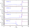 |
Fig. 8. Propagation of the shock through a low-density cavity bound by a high-density shell. The density is in units of mp cm−3. The dashed line shows the initial density profile, while the blue line shows the density profile evolution. When the forward shock moves through the low-density gas, the reverse shock moves outward. After the collision with the dense shell, the reverse shock propagates deep into the ejecta. These simulations are non-radiative, which is a reasonable approximation for the ejecta and the cavity. The forward shock in the dense gas is radiative; that is, its structure is not correctly reproduced by these simulations. A jump at 20 pc in the upper panel is the reflected reverse shock that appears in a spherically symmetric 1D model. |
The time evolution of the gas density over 35 kyr is shown in Fig. 8. Due to the very low density in the cavity, the ejecta almost freely expand over the first ∼10 kyr. During this period, the reverse shock is not very prominent and the bulk of the ejecta remains cold (see the bottom panel in Fig. 8). Once the ejecta reach the dense shell, a strong reverse shock starts propagating inward and eventually reaches the center (the two middle panels in the same figure). The final stage features a cavity filled with hot and low-density gas (a mixture of the ejecta and the initial gas content of the cavity) and a forward shock slowly propagating through the cold dense shell. This forward shock can have a complicated structure depending on the properties of the shell. In the scenario considered here, the forward shock powers the Hα filaments of S147, while the hot gas in the cavity produces X-ray emission.
While the parameters used in the model might not match the properties of the S147 progenitor and environment accurately, it is interesting to compare the X-ray spectra expected in this simple model with the data. This can be done in several steps. One needs to calculate the time evolution of the electron temperature in each radial shell, evolve ionization fractions, calculate the energy-dependent emissivity, and integrate it along the line of sight. To this end, we followed the same approach as in Churazov et al. (2021), Khabibullin et al. (2023). Here, for spectra calculations, the MEKAL model (Mewe et al. 1985; Liedahl et al. 1995) implemented in the XSPEC package (Arnaud 1996) was used in combination with the evolving ion fractions. For the electron temperature, the following three cases have been considered.
-
Te(r, t) = Th(r, t), where r and t are the shell radius and time, respectively, and Th(r, t) is the fluid temperature in the hydro run for a reasonable choice of the mean molecular weight, μ. This case corresponds to the equal temperature of all particles (the blue line in Fig. 9).
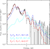
Fig. 9. SNR spectra based on the 1D hydro model shown in Fig. 8 at t = 3 × 10⁴ yr. The black crosses are the same data points as in Fig. 5. The models (blue, cyan, and red curves) differ in the level of deviation from the CIE state with Te = Ti. In particular, the blue curve corresponds to instantaneous electron and proton temperature equilibration (that is, Te = Tp = Ti) and the self-consistently calculated evolution of the ionization balance. The cyan curve shows the case when the rate of all collisional processes is artificially increased by a factor of 100 (i.e., this case is close to the CIE state with Te = Ti). The red curve shows the case in which most of the energy downstream of the shock goes into protons, and the electron and proton equilibration proceeds via pure Coulomb collisions. In all cases, the ionization balance is followed in each shell according to the time evolution of the electron temperature. The model spectra were integrated along the line of sight at a projected distance of 0.35 times the radius of the SNR.
-
In the second case, we assume that most of the energy downstream of the shock goes into protons, and that electron and proton equilibration proceeds via pure Coulomb collisions (the red line).
-
Finally, the last model also involves Coulomb collisions, but the rate of collisions is artificially increased by a factor of 100 (the cyan line). This model is expected to be close to the first model.
-
For the second version of the model-spectrum plot: finally, the last model assumes that Te(r, t) = Th(r, t), similar to the first model, but the rates of ionization and recombination are artificially increased by a factor of 100 (the cyan line). This model is expected to be closer to CIE than other models.
Fig. 9 shows that the second model fits the data surprisingly well, given the simplicity of the model. In this figure, the model spectrum corresponds to the projected distance, rp = 0.35rs, from the center of the SNR, where rs is the forward shock radius, although the dependence on the value of rp is rather weak. For the solar abundance of heavy elements, the normalization of the predicted surface brightness is a factor of ∼2 lower than the observed spectrum. Increasing abundance in the model by a factor of two brings the model very close to the observed spectrum. Large values of the abundance would overpredict the flux. As follows from Fig. 10, the full mixing scenario with the small amount of mass (used in our 1D model) would lead to a larger abundance of oxygen. This suggests that in S147 most of the X-ray emission is associated with the outer layers of the ejecta. The total energy “problem” apparent in Fig. 10 is easily resolved in the model with Ti ≫ Te, with the standard rates of temperature equilibration via Coulomb collisions.
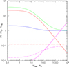 |
Fig. 10. Dependence of the mean temperature (the solid red line) and He (blue) and O (green) abundances when ejecta are mixed with a given mass (Madd) of the ISM. For the temperature calculations, we assume that the initial energy, E = 1051 erg, goes entirely into the gas heating, which is fully ionized. For the abundance calculation, we assume solar abundances for the ISM and the 1B-M20 model for the ejecta. For comparison, the dashed horizontal line is the best-fitting temperature for a one-temperature APEC model. The intersection of the dashed and solid red lines suggests a large added mass of ∼2 − 3 × 10³ M⊙. Similarly, the dashed magenta line shows the density derived from the normalization of the same model, taking into account the variable abundance of elements (focusing on O). The intersection of the dashed and solid magenta lines suggests a much smaller added mass of ∼102 M⊙. This discrepancy clearly demonstrates that the above set of assumptions (CIE, APEC spectral model, complete mixing of the ejecta and the gas inside the cavity, and Te = Ti) is likely violated. |
The shell model adopted here has an interesting implication for the temperature and ionization structure of the SNR seen in X-rays. Indeed, since much of the X-ray emission is expected to come from the gas reheated by the reverse shock, the profile of the ionization parameter, τ = ∫ndt, can be different from the standard case of a Sedov-like solution, in which the forward shock is responsible for X-ray emission. This is illustrated in Fig. 11, which shows the radial profiles of τ for S147 and G116-26.1. The latter is used to illustrate the forward-shock-dominated model, when the ambient medium is uniform. The same PLUTO code was used for this problem [see][for details on the initial conditions]2021MNRAS.507..971C. In both cases, the calculation of τ for a given fluid element begins when this fluid element goes through a shock and is heated to temperatures of ∼1 keV.
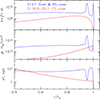 |
Fig. 11. Radial profile of the ionization parameter, τ = ∫ndt (blue line, top panel) based on the 1D model, in which most of the X-ray emission is coming from the gas reheated by the reverse shock following the collision of the ejecta with the dense shell. The radius is normalized by the characteristic radius, r0, which is approximately equal to the radius of the forward shock. Small amplitude irregularities in the black curve at r/r0 ≲ 0.8 are an artifact of τ calculations. For comparison, the red curve shows the case in which the X-ray emission is mostly due to the gas heated by the forward shock (the parameters for G116-26.1 are used here). Two spikes in τ are clearly visible at large radii. The outmost spike is likely an artifact of our non-radiative run near the inner boundary of the dense shell. The other spike is due to the less-dense gas (outer layers of ejecta) that has a relatively high temperature and can contribute to X-ray emission. In this region, oxygen might be completely ionized, but the lines of Si and Fe might be present, as is illustrated in Fig. 12. The middle and bottom panels compare the model density and temperature profiles for these two SNRs. |
For S147, the value of τ is almost constant through the entire ejecta, unlike the G116-26.1 case. In addition, S147 might have a spike in τ behind the position of the forward shock, due to the outer layers of ejecta that were reheated by the second reverse shock (see Fig. 8). Depending on the initial gas density in the cavity, such a spike might arise due to this gas. What is needed is a moderately dense gas that can be reheated by a reverse shock to high temperatures. This combination of parameters would drive τ up and power X-ray emission. If this model is correct, near the limb of S147 one can expect to find hotter and more highly ionized gas than in the rest of the nebula. This is illustrated in Fig. 12.
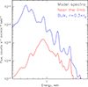 |
Fig. 12. Projected model spectra for the SN-in-the-WBB scenario near the limb (red) and toward the inner parts of the nebula (blue). The gas near the limb has a larger ionization parameter than the bulk of the volume and accordingly lacks oxygen lines, but features the lines of Ne, Fe, and Si. In reality, S147 is far from spherical symmetry and a mixture of components with a range of ionization parameters should be observed. |
4.7. Abundances
Most of the above analysis was done assuming solar abundance (or solar mix of abundances) in the X-ray emitting gas. As is illustrated by Figs. 7 and 10, the abundance of oxygen relative to hydrogen is sensitive to the amount of “cavity gas” added to the ejecta and to the assumption that entire ejecta are mixed with this gas and all this gas contributes to the observed X-ray emission. Given the complexity of S147, this is likely a severe simplification. On the other hand, the variations in abundances relative to oxygen are less extreme, in the range of 0.3–2 for elements from C to Fe, when averaged over the entire ejecta. Fig. 13 shows the contributions of individual elements to the NEI model with solar abundances. Clearly, the underabundance of C and N in the adopted ejecta model might affect the absorbing column density derived from the X-ray spectra. For the heavier elements, like Ne, Mg, and Si, an uncertainty factor of ∼2 (or larger) is feasible. Our conclusion here is that allowing abundance variations, coupled with uncertainties in Te and nonequilibrium ionization, would allow for an even better fit to the observed X-ray spectra, although the degeneracy between parameters would lead to large uncertainties in the derived parameters.
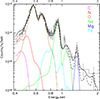 |
Fig. 13. Contribution of individual elements to the S147 X-ray spectrum in the NEI model (solid black line). The dashed line shows the spectrum predicted by the 1D-hydro model. |
4.8. Nonthermal components in S147
While no signature of nonthermal X-rays was found in the eROSITA data analysis, it is still worth discussing the presence of nonthermal components in multiwavelength data, since these are needed to justify the SNR model presented above. Indeed, the shocks of velocity ≳100 km s−1 in the current stage of S147 evolution are not fast enough to allow particle acceleration above TeV energies with magnetic field amplification, which is needed to extend the synchrotron radiation spectra to X-rays, in contrast to the case of young SNRs (see e.g. Bykov et al. 2018; Vink 2020). However, GeV regime electrons and protons can be accelerated and confined in S147, providing the observed radio and gamma-ray emission, and may contain a sizable energy density that is ∼10% of the total gas pressure.
The radio image of S147 is composed of “filaments,” associated with Hα filaments, and a diffuse component. The appearance of the radio filaments has the same origin as the Hα filaments; the limb brightening. The overall integrated flux density is 34.8 ± 4 Jy at 11 cm (Xiao et al. 2008). The spectrum is flat (α = −0.30 ± 0.15, F ∝ να) in the range of ≲1.5 GHz and gets steeper at higher frequencies (Xiao et al. 2008). The observed flux at 11 cm can be described based on a simple model of a homogeneous spherical radio-emitting shell filled with cosmic rays and magnetic fields. The outer radius of the SNR is R2 = 39 pc and the inner radius R1 = 0.9R2 (adopting the SNR distance of 1.3 kpc). For initial estimations, one can assume an equipartition between cosmic rays and the magnetic field energy density (Ucr = B2/8π) with a typical electron-to-proton ratio of ξe, p = Ue/Up = 0.01. The energy spectrum of relativistic electrons responsible for the radio emission is assumed to be dN/dE = KE−p, with p = 2 in the GeV range, consistent with that expected in the diffusive shock acceleration (DSA) model.
The observed flux at 11 cm is then reproduced for the total energy of the relativistic component, Erel = 9 × 1049 erg, suggesting an energy density of Urel ≈ 4.5 × 10⁻¹¹ erg cm−3 and a magnetic field of about 24 μG. Remarkably, the relativistic pressure in this model, prel ≈ 1.5 × 10⁻¹¹ dyn cm−2, turns out to be a sizable fraction of the upstream dynamical pressure. Indeed, for vs = 100 km s−1 and a pre-shock density of n0 = 0.3 cm−3, the dynamical pressure is pdyn = ρ0v2 ≈ 7 × 10⁻¹¹ dyn cm−2, with the ratio ξ = prel/pdyn = 0.2. The estimates above assume a homogeneous radio-emitting shell, while the radio images reveal a filamentary structure of the SNR, probably indicating a highly intermittent structure of magnetic fields, which can be probed by combining radio and gamma-ray data.
The nonthermal pressure estimated from radio emission of relativistic electrons in the SNR can be compared with the one derived from the gamma-ray data. Fermi-LAT observations of S147 by Katsuta et al. (2012) in the energy range of 0.2–10 GeV revealed an extended gamma-ray source of luminosity of ∼1.3 × 1034 erg s−1 at the assumed distance of 1.3 kpc. They pointed out an apparent correlation of the gamma-ray emission with the Hα filaments and found no signal associated with the pulsar PSR J0538+2817. These authors concluded that reacceleration and further compression of the preexisting cosmic rays can explain the gamma-ray data. Within the hadronic scenario of the S147 gamma-ray origin, the derived gamma-ray luminosity would correspond to a total energy in cosmic ray protons of ∼1049/na ergs (where na, which is measured in cm−3, is the average number density of the gas in a single zone homogeneous model). Later on, Suzuki et al. (2022) obtained the 1–100 GeV Fermi-LAT gamma-ray luminosity of S147, ∼6 × 1032 erg s−1, and the spectrum was fitted with a broken power law model. Below the break energy at ∼1.4 GeV, the photon index of about 2.14–2.18 was found, while a much softer spectrum (with the photon index of ∼3.9) was found above the break, extending down to the cutoff energies of > 21 GeV. The radio spectrum discussed above is broadly consistent with that of the low-energy gamma rays, bearing in mind that the momentum distributions of both electrons and protons accelerated by DSA are expected to have the same power law index (of about two) in the GeV energy range. The break in the gamma-ray spectrum at 1.4 GeV detected by Fermi-LAT within the hadronic model roughly corresponds to a break in the proton spectrum at about 14 GeV. Then, assuming that the electron spectrum has a break at the same energy from the position of the break frequency in the radio spectrum given by Xiao et al. (2008), one can estimate the magnetic field in the diffuse emission to be about μG. If both the filaments and diffuse regions are embedded in a single population of electrons accelerated via the DSA process, then the lack of observed break in the radio filaments till 40 GHz implies that the magnetic fields there are above 40 μG.
5. Discussion
Several generic scenarios of the “supernova-in-a-cavity” type have been modeled before (e.g. Tenorio-Tagle et al. 1990) and suggested for S147 (e.g. Reich et al. 2003). Here, to make the formulation of the model more complete, we assume that the cavity is created by the winds of a sufficiently massive star during its MS evolutionary phase. The presence of the pulsar and the size of the Hα nebula together suggest a progenitor mass of order 20 M⊙, leading to a well-constrained model. It appears that this model can explain many X-ray properties of S147. In particular, this model naturally predicts X-ray spectra that feature lines of Mg and Si along with the lines of OVII and OVII, and does not require excess low-energy absorption. It also predicts that the X-ray emitting gas extends all the way to the Hα-emitting shell.
We note here that a qualitatively similar picture is expected if the cavity, needed to reduce the SNR age, is produced by another mechanism rather than MS-driven WBB (e.g. Gvaramadze 2006). As long as the mass of the dense shell is large and the cavity is filled with low-density gas, most of the conclusions stay unchanged. From this point of view, the only important parameter for modeling the expected X-ray emission is the observed size of the SNR, which in this model is essentially the original size of the cavity.
A natural implication of this model is that the ions in the interior of the dense shell are much hotter than the electrons and that the ionization equilibrium is not achieved. A direct test of these predictions should be possible with forthcoming X-ray bolometers like XRISM (XRISM Science Team 2020), ATHENA (Nandra et al. 2013), and LEM (Kraft et al. 2022). The detection of very broad lines of O, Ne, Mg, and Si ions would be a decisive test of the “hot” S147 scenario. A lack of broadening would instead support the “cold” model. For the time being, S147 can be considered a promising candidate for the list of objects featuring Ti ≫ Te (e.g. Raymond et al. 2023). Constraints on weaker lines, for example Fe XVII, from forthcoming bolometers would also tighten the constraints on the NEI models.
As a caveat, we mention that it is not entirely clear if the modest abundance enhancement inferred from the observed flux of the NEI plasma represents a serious challenge to the hot model. Potentially, the abundance can be much higher. Yet another simplification used here is the assumption of spherical symmetry, which clearly does not apply to S147.
Another interesting question is how often one could find SN II exploded inside the WBB. The answer depends on the progenitor velocity (v*) relative to the ISM. The dispersion velocity of OB-stars is ∼10 km s−1, (Bobylev et al. 2022), although the well-known RSG Betelgeuse (M ∼ 15 M⊙) shows an even larger velocity with respect to the ISM, v* ≈ 30 km s−1 (Ueta et al. 2008). The 20 M⊙ star with a velocity of 10 km s−1 with respect to the ISM will run 80 pc to the end of the MS lifetime and will reside near the bubble frontal boundary at a distance comparable to the termination shock radius (∼3 pc). In the subsequent helium-burning stage (0.8 × 10⁶ yr), the star will run another 8 pc and escape the bubble. We conclude that most SNe II explode outside their WBBs and that S147 should be considered as a rare example of an SN II that exploded in the WBB presumably owing to the low progenitor velocity with respect to the ISM. This might explain a highly unusual Hα appearance of S147, although the Vela SNR seems to show a somewhat similar Hα pattern (see Gvaramadze 1999 for a discussion of SNR-in-cavity scenario for the Vela SNR). Yet in Vela we do not see ring-like structures in the central part of the SNR, unlike in S147, which suggests that Vela and S147 are not identical. Interestingly, a finite progenitor velocity of ∼1 km s−1 could result in the SN offset with respect to the bubble center (Mackey et al. 2015), which in turn could also bring about the observed deviations from sphericity of S147.
In the model discussed here, the age estimate based on the kinematics of the pulsar J0538+2817 broadly agrees with the observed characteristics of S147. This strengthens the association of the pulsar with the SN. This implies that the pulsar is plausibly inside the SNR and might affect its properties. Some tantalizing hints might be spotted in Fig. 4. This will be the subject of a separate study.
6. Conclusions
We argue that new X-ray data of SRG/eROSITA lends support to S147 being a type II SN that exploded in a low-density cavity. The main features of this scenario can be summarized as follows.
-
The SN going off in a cavity that was formed during MS stage of a star of ∼20 M⊙ is a plausible scenario for the formation of the cavity.
-
This star had a relatively small velocity relative to the ambient ISM. As a result, a dense shell around the cavity is approximately spherical and the SN explosion was not far from its center.
-
The age is consistent with that derived from the kinematics of the pulsar PSR J0538+2817 (∼35 kyr).
-
The X-ray emission comes predominantly from the gas inside the cavity. The gas there has Te ≪ Ti and is not in CIE. This gas was reheated by reverse shock following the collision of the ejecta with the dense shell. A large fraction of ejecta kinetic energy is “reflected” by the shell back into the cavity.
-
The Hα and narrow radio filaments are associated with the radiative forward shock that propagates through the dense shell.
-
Diffuse radio is due to the particles that were accelerated at the radiative shocks, but that now exist in an environment with a much weaker magnetic field.
-
The eventual fate of an SNR in the cavity is to become a hot and low-density gas bubble (no oxygen lines) until that dissolves in the ISM.
-
Other scenarios for the cavity formation might be consistent with X-ray data, as long as the mass of the dense shell is large.
Finally, we note that S147 has a very complicated morphology and spectra from radio to gamma-rays and that the above model is not intended to reproduce all this complexity. However, we believe that it captures some of the essential features of this remarkable SNR.
Acknowledgments
This work is partly based on observations with the eROSITA telescope onboard SRG space observatory. The SRG observatory was built by Roskosmos in the interests of the Russian Academy of Sciences represented by its Space Research Institute (IKI) in the framework of the Russian Federal Space Program, with the participation of the Deutsches Zentrum für Luft- und Raumfahrt (DLR). The eROSITA X-ray telescope was built by a consortium of German Institutes led by MPE, and supported by DLR. The SRG spacecraft was designed, built, launched, and is operated by the Lavochkin Association and its subcontractors. The science data are downlinked via the Deep Space Network Antennae in Bear Lakes, Ussurijsk, and Baikonur, funded by Roskosmos. The development and construction of the eROSITA X-ray instrument was led by MPE, with contributions from the Dr. Karl Remeis Observatory Bamberg & ECAP (FAU Erlangen-Nuernberg), the University of Hamburg Observatory, the Leibniz Institute for Astrophysics Potsdam (AIP), and the Institute for Astronomy and Astrophysics of the University of Tübingen, with the support of DLR and the Max Planck Society. The Argelander Institute for Astronomy of the University of Bonn and the Ludwig Maximilians Universität Munich also participated in the science preparation for eROSITA. The eROSITA data were processed using the eSASS/NRTA software system developed by the German eROSITA consortium and analysed using proprietary data reduction software developed by the Russian eROSITA Consortium. IK acknowledges support by the COMPLEX project from the European Research Council (ERC) under the European Union’s Horizon 2020 research and innovation program grant agreement ERC-2019-AdG 882679. A.M.B. was supported by the RSF grant 21-72-20020. His modeling was performed at the Joint Supercomputer Center JSCC RAS and at the Peter the Great Saint-Petersburg Polytechnic University Supercomputing Center. Rashid Sunyaev acknowledges the support of dvp – N/A pertaining to Member Notification Merge at the Institute for Advanced Study. This research made use of Montage (http://montage.ipac.caltech.edu). It is funded by the National Science Foundation under Grant Number ACI-1440620, and was previously funded by the National Aeronautics and Space Administration’s Earth Science Technology Office, Computation Technologies Project, under Cooperative Agreement Number NCC5-626 between NASA and the California Institute of Technology.
References
- Anderson, S. B., Cadwell, B. J., Jacoby, B. A., et al. 1996, ApJ, 468, L55 [Google Scholar]
- Arnaud, K. A. 1996, ASP Conf. Ser., 101, 17 [Google Scholar]
- Bertoldi, F., & McKee, C. F. 1990, ApJ, 354, 529 [NASA ADS] [CrossRef] [Google Scholar]
- Blondin, J. M., Wright, E. B., Borkowski, K. J., & Reynolds, S. P. 1998, ApJ, 500, 342 [Google Scholar]
- Bobylev, V. V., Bajkova, A. T., & Karelin, G. M. 2022, Astron. Lett., 48, 243 [NASA ADS] [CrossRef] [Google Scholar]
- Bykov, A. M., Ellison, D. C., Marcowith, A., & Osipov, S. M. 2018, Space Sci. Rev., 214, 41 [CrossRef] [Google Scholar]
- Chatterjee, S., Brisken, W. F., Vlemmings, W. H. T., et al. 2009, ApJ, 698, 250 [NASA ADS] [CrossRef] [Google Scholar]
- Chevalier, R. A., & Liang, E. P. 1989, ApJ, 344, 332 [NASA ADS] [CrossRef] [Google Scholar]
- Churazov, E. M., Khabibullin, I. I., Bykov, A. M., et al. 2021, MNRAS, 507, 971 [NASA ADS] [CrossRef] [Google Scholar]
- Cox, D. P. 2005, ARA&A, 43, 337 [Google Scholar]
- Denoyer, L. K. 1974, AJ, 79, 1253 [NASA ADS] [CrossRef] [Google Scholar]
- Dickey, J. M., & Garwood, R. W. 1989, ApJ, 341, 201 [NASA ADS] [CrossRef] [Google Scholar]
- Dwarkadas, V. V. 2023, Galaxies, 11, 78 [NASA ADS] [CrossRef] [Google Scholar]
- Fuerst, E., & Reich, W. 1986, A&A, 163, 185 [NASA ADS] [Google Scholar]
- Gaze, V. F., & Shajn, G. A. 1952, Izvestiya Krymskoj Astrofizicheskoj Observatorii, 9, 52 [NASA ADS] [Google Scholar]
- Greimel, R., Drew, J. E., Monguió, M., et al. 2021, A&A, 655, A49 [NASA ADS] [CrossRef] [EDP Sciences] [Google Scholar]
- Gvaramadze, V. 1999, A&A, 352, 712 [NASA ADS] [Google Scholar]
- Gvaramadze, V. V. 2006, A&A, 454, 239 [NASA ADS] [CrossRef] [EDP Sciences] [Google Scholar]
- Heger, A., Fryer, C. L., Woosley, S. E., Langer, N., & Hartmann, D. H. 2003, ApJ, 591, 288 [CrossRef] [Google Scholar]
- Heyer, M., & Dame, T. M. 2015, ARA&A, 53, 583 [Google Scholar]
- Howarth, I. D., & Prinja, R. K. 1989, ApJS, 69, 527 [NASA ADS] [CrossRef] [Google Scholar]
- Hughes, J. P. 1987, ApJ, 314, 103 [NASA ADS] [CrossRef] [Google Scholar]
- Katsuta, J., Uchiyama, Y., Tanaka, T., et al. 2012, ApJ, 752, 135 [NASA ADS] [CrossRef] [Google Scholar]
- Khabibullin, I. I., Churazov, E. M., Bykov, A. M., Chugai, N. N., & Sunyaev, R. A. 2023, MNRAS, 521, 5536 [NASA ADS] [CrossRef] [Google Scholar]
- Khabibullin, I. I., Churazov, E. M., Bykov, A. M., Chugai, N. N., & Zinchenko, I. I. 2024, MNRAS, 527, 5683 [Google Scholar]
- Kirshner, R. P., & Arnold, C. N. 1979, ApJ, 229, 147 [Google Scholar]
- Kochanek, C. S., Raymond, J. C., Caldwell, N., et al. 2024, arXiv e-prints [arXiv:2403.13892] [Google Scholar]
- Kraft, R., Markevitch, M., Kilbourne, C., et al. 2022, ArXiv e-prints [arXiv:2211.09827] [Google Scholar]
- Kramer, M., Lyne, A. G., Hobbs, G., et al. 2003, ApJ, 593, L31 [Google Scholar]
- Larson, R. B. 1981, MNRAS, 194, 809 [Google Scholar]
- Liedahl, D. A., Osterheld, A. L., & Goldstein, W. H. 1995, ApJ, 438, L115 [CrossRef] [Google Scholar]
- Lozinskaia, T. A. 1976, AZh, 53, 38 [Google Scholar]
- Mackey, J., Gvaramadze, V. V., Mohamed, S., & Langer, N. 2015, A&A, 573, A10 [NASA ADS] [CrossRef] [EDP Sciences] [Google Scholar]
- Martizzi, D., Faucher-Giguère, C.-A., & Quataert, E. 2015, MNRAS, 450, 504 [NASA ADS] [CrossRef] [Google Scholar]
- Mewe, R., Gronenschild, E. H. B. M., & van den Oord, G. H. J. 1985, A&AS, 62, 197 [NASA ADS] [Google Scholar]
- Michailidis, M., Pühlhofer, G., Becker, W., et al. 2024, A&A, 689, A277 (Paper I) [NASA ADS] [CrossRef] [EDP Sciences] [Google Scholar]
- Mignone, A., Bodo, G., Massaglia, S., et al. 2007, ApJS, 170, 228 [Google Scholar]
- Nandra, K., Barret, D., Barcons, X., et al. 2013, ArXiv e-prints [arXiv:1306.2307] [Google Scholar]
- Ng, C. Y., Romani, R. W., Brisken, W. F., Chatterjee, S., & Kramer, M. 2007, ApJ, 654, 487 [NASA ADS] [CrossRef] [Google Scholar]
- Pikel’ner, S. 1954, Izvestiya Ordena Trudovogo Krasnogo Znameni Krymskoj Astrofizicheskoj Observatorii, 12, 93 [Google Scholar]
- Predehl, P., Andritschke, R., Arefiev, V., et al. 2021, A&A, 647, A1 [EDP Sciences] [Google Scholar]
- Raymond, J. C., Ghavamian, P., Bohdan, A., et al. 2023, ApJ, 949, 50 [NASA ADS] [CrossRef] [Google Scholar]
- Reich, W., Zhang, X., & Fürst, E. 2003, A&A, 408, 961 [NASA ADS] [CrossRef] [EDP Sciences] [Google Scholar]
- Ren, J.-J., Liu, X.-W., Chen, B.-Q., et al. 2018, RAA, 18, 111 [Google Scholar]
- Romani, R. W., & Ng, C. Y. 2003, ApJ, 585, L41 [Google Scholar]
- Schaller, G., Schaerer, D., Meynet, G., & Maeder, A. 1992, A&AS, 96, 269 [Google Scholar]
- Silk, J., & Wallerstein, G. 1973, ApJ, 181, 799 [NASA ADS] [CrossRef] [Google Scholar]
- Sofue, Y., Furst, E., & Hirth, W. 1980, PASJ, 32, 1 [NASA ADS] [Google Scholar]
- Sunyaev, R., Arefiev, V., Babyshkin, V., et al. 2021, A&A, 656, A132 [NASA ADS] [CrossRef] [EDP Sciences] [Google Scholar]
- Sutherland, R. S., & Dopita, M. A. 1993, ApJS, 88, 253 [Google Scholar]
- Suzuki, H., Bamba, A., Yamazaki, R., & Ohira, Y. 2022, ApJ, 924, 45 [NASA ADS] [CrossRef] [Google Scholar]
- Taylor, A. R., Gibson, S. J., Peracaula, M., et al. 2003, AJ, 125, 3145 [NASA ADS] [CrossRef] [Google Scholar]
- Tenorio-Tagle, G., Bodenheimer, P., Franco, J., & Rozyczka, M. 1990, MNRAS, 244, 563 [NASA ADS] [Google Scholar]
- Tenorio-Tagle, G., Rozyczka, M., Franco, J., & Bodenheimer, P. 1991, MNRAS, 251, 318 [NASA ADS] [CrossRef] [Google Scholar]
- Ueta, T., Izumiura, H., Yamamura, I., et al. 2008, PASJ, 60, S407 [NASA ADS] [Google Scholar]
- Utrobin, V. P., Wongwathanarat, A., Janka, H.-T., & Müller, E. 2017, ApJ, 846, 37 [NASA ADS] [CrossRef] [Google Scholar]
- Vink, J. 2020, Physics and Evolution of Supernova Remnants (Springer Nature) [CrossRef] [Google Scholar]
- Weaver, R., McCray, R., Castor, J., Shapiro, P., & Moore, R. 1977, ApJ, 218, 377 [Google Scholar]
- Woosley, S. E., Heger, A., & Weaver, T. A. 2002, Rev. Mod. Phys., 74, 1015 [NASA ADS] [CrossRef] [Google Scholar]
- Xiao, L., Fürst, E., Reich, W., & Han, J. L. 2008, A&A, 482, 783 [NASA ADS] [CrossRef] [EDP Sciences] [Google Scholar]
- XRISM Science Team 2020, ArXiv e-prints [arXiv:2003.04962] [Google Scholar]
All Tables
Simplest spectral model fits to the spectrum of the entire SNR in the 0.4–3 keV band.
All Figures
|
Fig. 1. Broadband (0.5–1.0 keV) (particle) background-subtracted, exposure-corrected X-ray image (linear scale) obtained by SRG/eROSITA in the S147 direction (3.7° × 3.7° in Galactic coordinates) after masking of point and mildly extended sources and smoothing with a Gaussian kernel with σ = 1′. This band maximizes the source-to-background ratio for the SNR emission. The cross marks the position of the pulsar PSR. |
| In the text | |
|
Fig. 2. Multiwavelength view of S147 (in Galactic coordinates). Top: combined map of the radio (CGPS data at 1.4 GHz, red), wavelet-decomposed (in order to emphasize filamentary structure) Hα (IGAPS data, green), and broadband X-ray (0.5–1.1 keV, SRG/eROSITA data, blue) emission. The white cross marks the position of PSR J0538+2817. Middle: the intensity-saturated X-ray image is shown in blue on top of the wavelet-decomposed Hα image, demonstrating that X-ray emission is confined by the Hα-emitting shell. Bottom: same as the middle panel but with the 1.4 GHz radio emission as a background. |
| In the text | |
|
Fig. 3. X-ray spectrum of the whole remnant (red data points) after subtraction of the background signal (blue data points) estimated from an adjacent sky region. Also shown is the level of 10% of the background emission, which aims to show that above 1.5 keV the SN signal amounts to a few % of the background level, making conclusions regarding its spectral shape at these energies strongly background-sensitive. The three bands containing the brightest emission lines are shown in red (O VII), green (O VII), and blue (Ne IX), and are used for RGB composite images. |
| In the text | |
|
Fig. 4. RGB-composite (top left) and individual narrow-band X-ray images covering the 0.44–1.1 keV band. The red, green, and cyan (instead of blue, for better visibility) images correspond to the 0.44–0.62, 0.62–0.8, and 0.8–1.1 keV bands, respectively. These bands encompass the three brightest X-ray emission lines in the spectrum of S147: O VII, O VIII, and Ne IX. |
| In the text | |
|
Fig. 5. X-ray spectrum of the entire S147 SNR. The red line shows the best-fitting APEC model (single-temperature, CIE, solar abundance of metals). This model requires a very large absorbing column density, overpredicts the flux near 0.8 keV (where a significant contribution of Fe XVII line at 826 eV is expected), and underpredicts the Mg XI line flux unless its abundance (relative to oxygen) is very high. For comparison, the blue line shows the NEI model with parameters fixed at physically motivated values. Although formally the value of χ2 is higher than for the APEC model, the lower value of NH and the ability of the model to better describe regions near Fe XVII and Mg XI lines make this model an appealing interpretation of the S147 spectrum (see text for details). |
| In the text | |
|
Fig. 6. Radius of the wind-driven bubble formed by the 20 M⊙ star wind at the MS. The lines are labeled according to the ISM pressure. The model with zero pressure shows the bubble radius based on the analytic solution (Weaver et al. 1977). |
| In the text | |
|
Fig. 7. Ejecta structure for the 1B-M20 model. The solid black line shows the enclosed ejecta mass (for a given velocity). The dashed colored lines show which velocities make the largest contribution to the mass of a given element; namely, the quantity 4πr3ρi, where ρi is the mass density of the i-th element, color-coded as in the legend. The solid colored lines show the mass density of the i-th element relative to the mass density of oxygen, normalized by the solar value. |
| In the text | |
|
Fig. 8. Propagation of the shock through a low-density cavity bound by a high-density shell. The density is in units of mp cm−3. The dashed line shows the initial density profile, while the blue line shows the density profile evolution. When the forward shock moves through the low-density gas, the reverse shock moves outward. After the collision with the dense shell, the reverse shock propagates deep into the ejecta. These simulations are non-radiative, which is a reasonable approximation for the ejecta and the cavity. The forward shock in the dense gas is radiative; that is, its structure is not correctly reproduced by these simulations. A jump at 20 pc in the upper panel is the reflected reverse shock that appears in a spherically symmetric 1D model. |
| In the text | |
|
Fig. 9. SNR spectra based on the 1D hydro model shown in Fig. 8 at t = 3 × 10⁴ yr. The black crosses are the same data points as in Fig. 5. The models (blue, cyan, and red curves) differ in the level of deviation from the CIE state with Te = Ti. In particular, the blue curve corresponds to instantaneous electron and proton temperature equilibration (that is, Te = Tp = Ti) and the self-consistently calculated evolution of the ionization balance. The cyan curve shows the case when the rate of all collisional processes is artificially increased by a factor of 100 (i.e., this case is close to the CIE state with Te = Ti). The red curve shows the case in which most of the energy downstream of the shock goes into protons, and the electron and proton equilibration proceeds via pure Coulomb collisions. In all cases, the ionization balance is followed in each shell according to the time evolution of the electron temperature. The model spectra were integrated along the line of sight at a projected distance of 0.35 times the radius of the SNR. |
| In the text | |
|
Fig. 10. Dependence of the mean temperature (the solid red line) and He (blue) and O (green) abundances when ejecta are mixed with a given mass (Madd) of the ISM. For the temperature calculations, we assume that the initial energy, E = 1051 erg, goes entirely into the gas heating, which is fully ionized. For the abundance calculation, we assume solar abundances for the ISM and the 1B-M20 model for the ejecta. For comparison, the dashed horizontal line is the best-fitting temperature for a one-temperature APEC model. The intersection of the dashed and solid red lines suggests a large added mass of ∼2 − 3 × 10³ M⊙. Similarly, the dashed magenta line shows the density derived from the normalization of the same model, taking into account the variable abundance of elements (focusing on O). The intersection of the dashed and solid magenta lines suggests a much smaller added mass of ∼102 M⊙. This discrepancy clearly demonstrates that the above set of assumptions (CIE, APEC spectral model, complete mixing of the ejecta and the gas inside the cavity, and Te = Ti) is likely violated. |
| In the text | |
|
Fig. 11. Radial profile of the ionization parameter, τ = ∫ndt (blue line, top panel) based on the 1D model, in which most of the X-ray emission is coming from the gas reheated by the reverse shock following the collision of the ejecta with the dense shell. The radius is normalized by the characteristic radius, r0, which is approximately equal to the radius of the forward shock. Small amplitude irregularities in the black curve at r/r0 ≲ 0.8 are an artifact of τ calculations. For comparison, the red curve shows the case in which the X-ray emission is mostly due to the gas heated by the forward shock (the parameters for G116-26.1 are used here). Two spikes in τ are clearly visible at large radii. The outmost spike is likely an artifact of our non-radiative run near the inner boundary of the dense shell. The other spike is due to the less-dense gas (outer layers of ejecta) that has a relatively high temperature and can contribute to X-ray emission. In this region, oxygen might be completely ionized, but the lines of Si and Fe might be present, as is illustrated in Fig. 12. The middle and bottom panels compare the model density and temperature profiles for these two SNRs. |
| In the text | |
|
Fig. 12. Projected model spectra for the SN-in-the-WBB scenario near the limb (red) and toward the inner parts of the nebula (blue). The gas near the limb has a larger ionization parameter than the bulk of the volume and accordingly lacks oxygen lines, but features the lines of Ne, Fe, and Si. In reality, S147 is far from spherical symmetry and a mixture of components with a range of ionization parameters should be observed. |
| In the text | |
|
Fig. 13. Contribution of individual elements to the S147 X-ray spectrum in the NEI model (solid black line). The dashed line shows the spectrum predicted by the 1D-hydro model. |
| In the text | |
Current usage metrics show cumulative count of Article Views (full-text article views including HTML views, PDF and ePub downloads, according to the available data) and Abstracts Views on Vision4Press platform.
Data correspond to usage on the plateform after 2015. The current usage metrics is available 48-96 hours after online publication and is updated daily on week days.
Initial download of the metrics may take a while.