| Issue |
A&A
Volume 691, November 2024
|
|
|---|---|---|
| Article Number | A133 | |
| Number of page(s) | 13 | |
| Section | Extragalactic astronomy | |
| DOI | https://doi.org/10.1051/0004-6361/202451490 | |
| Published online | 05 November 2024 | |
The ALMA-CRISTAL survey: Dust temperature and physical conditions of the interstellar medium in a typical galaxy at z = 5.66
1
Departamento de Astronomía, Universidad de Concepción, Barrio Universitario, Concepción, Chile
2
Instituto de Astrofísica, Facultad de Física, Pontificia Universidad Católica de Chile, Santiago, 7820436
Chile
3
Instituto de Estudios Astrofísicos, Facultad de Ingeniería y Ciencias, Universidad Diego Portales, Av. Ejército 441, Santiago, 8370191
Chile
4
National Radio Astronomy Observatory, 520 Edgemont Road, Charlottesville, VA, 22903
USA
5
INAF-Istituto di Radioastronomia, Via Gobetti 101, 40129 Bologna, Italy
6
Chemistry Department, Sapienza University of Rome, P.le A. Moro, 00185 Rome, Italy
7
Jodrell Bank Centre for Astrophysics, Department of Physics and Astronomy, School of Natural Sciences, The University of Manchester, Manchester, M13 9PL
UK
8
International Centre for Radio Astronomy Research, ICRAR M468, 35 Stirling Hwy, Crawley, 6009
Western Australia
9
Sterrenkundig Observatorium, Ghent University, Krijgslaan 281 - S9, B9000 Ghent, Belgium
10
Department of Physics & Astronomy, University College London, Gower Street, London, WC1E 6BT
UK
11
Institute of Astrophysics, Foundation for Research and Technology-Hellas (FORTH), Heraklion, GR-70013
Greece
12
School of Sciences, European University Cyprus, Diogenes street, Engomi, 1516 Nicosia, Cyprus
13
Max-Planck-Institut fuer extraterrestrische Physik, Giessenbachstrasse 1, 85748 Garching, Germany
14
Hiroshima Astrophysical Science Center, Hiroshima University, 1-3-1 Kagamiyama, Higashi-Hiroshima, 739-8526 Hiroshima, Japan
15
Department of Astronomy, School of Science, SOKENDAI (The Graduate University for Advanced Studies), 2-21-1 Osawa, Mitaka, Tokyo, 181-8588
Japan
16
Department of Astronomy, The University of Tokyo, 7-3-1 Hongo, Bunkyo, Tokyo, 113-0033
Japan
17
National Astronomical Observatory of Japan, 2-21-1 Osawa, Mitaka, Tokyo, 181-8588
Japan
18
Max Planck Institut für Astrophysik, Karl-Schwarzschild-Str. 1, D-85741 Garching, Germany
19
Departamento Física Teórica y del Cosmos, Universidad de Granada, E-18071 Granada, Spain
20
Instituto Universitario Carlos I de Física Teórica y Computacional, Universidad de Granada, E-18071 Granada, Spain
21
Department of Physics and Astronomy and George P. and Cynthia Woods Mitchell Institute for Fundamental Physics and Astronomy, Texas A&M University, 4242 TAMU, College Station, TX, 77843-4242
USA
22
Dipartimento di Fisica e Astronomia, Universita di Bologna, via Gobetti 93/2, I-40129 Bologna, Italy
23
INAF – OAS, Osservatorio di Astrofisica e Scienza dello Spazio di Bologna, via Gobetti 93/3, I-40129 Bologna, Italy
24
Department of Physics and Astronomy and PITT PACC, University of Pittsburgh, Pittsburgh, PA, 15260
USA
25
Faculty of Engineering, Hokkai-Gakuen University, Toyohira-ku, Sapporo, 062-8605
Japan
26
Kavli Institute for Cosmology, University of Cambridge, Madingley Road, Cambridge, CB3 0HA
UK
27
Cavendish Laboratory, University of Cambridge, 19 JJ Thomson Avenue, Cambridge, CB3 0HE
UK
28
Scuola Normale Superiore, Piazza dei Cavalieri 7, I- 50126 Pisa, Italy
29
Las Campanas Observatory, Carnegie Institution of Washington, Casilla 601, La Serena, Chile
⋆⋆ Corresponding author; This email address is being protected from spambots. You need JavaScript enabled to view it.
Received:
12
July
2024
Accepted:
18
September
2024
Abstract
We present new λrest = 77 μm dust continuum observations from the Atacama Large Millimeter/submillimeter Array of HZ10 (CRISTAL-22). This dusty main sequence galaxy at z = 5.66 was observed as part of the [CII] Resolved Ism in STar-forming Alma Large program (CRISTAL). The high angular resolution of the ALMA Band 7 and new Band 9 data (∼0′′.4) reveals the complex structure of HZ10, which comprises two main components (HZ10-C and HZ10-W), along with a bridge-like dusty emission between them (i.e., “the bridge”). Using a modified blackbody function to model the dust spectral energy distribution (SED), we constrained the physical conditions of the interstellar medium (ISM) and its variations among the different components identified in HZ10. We find that HZ10-W (the more UV-obscured component) has an SED dust temperature of TSED ∼ 51.2 ± 13.1 K; this was found to be ∼5 K higher (which is statistically insignificant; i.e., less than 1σ) than that of the central component and previous global estimations for HZ10. Our new ALMA data allow us to reduce the uncertainties of global TSED measurements by a factor of ∼2.3, compared to previous studies. The HZ10 components have [CII]-to-far-infrared (FIR) luminosity ratios and FIR surface densities values that are consistent with local starburst galaxies. However, HZ10-W shows a lower [CII]/FIR ratio compared to the other two components (albeit still within the uncertainties), which may suggest a harder radiation field destroying polycyclic aromatic hydrocarbon associated with [CII] emission (e.g., active galactic nuclei or young stellar populations). While HZ10-C appears to follow the tight IRX-βUV relation seen in local UV-selected starburst galaxies and high-z star-forming galaxies, we find that both HZ10-W and the bridge depart from this relation and are well described by dust-screen models with holes in front of a hard UV radiation field. This suggests that the UV emission, which is likely coming from young stellar populations, is strongly attenuated in the “dustier” components of the HZ10 system.
Key words: galaxies: distances and redshifts / galaxies: evolution / galaxies: formation / galaxies: high-redshift / galaxies: structure
ALMA-ANID Postdoctoral Fellow.
© The Authors 2024
 Open Access article, published by EDP Sciences, under the terms of the Creative Commons Attribution License (https://creativecommons.org/licenses/by/4.0), which permits unrestricted use, distribution, and reproduction in any medium, provided the original work is properly cited.
This article is published in open access under the Subscribe to Open model. This email address is being protected from spambots. You need JavaScript enabled to view it. to support open access publication.
1. Introduction
Accurate measurements of dust temperatures (Tdust) in star-forming main sequence galaxies are critical to determine their infrared luminosities (LIR), star formation rates (SFRs), and dust attenuation properties (e.g., the excess of infrared emission compared to the ultra-violet, UV, or Balmer decrement, among others), which are fundamental quantities in the context of galaxy evolution. However, precise estimations of Tdust require the detection of the dust continuum emission from both sides of the peak of the infrared spectral energy distribution (SED; e.g., Hodge & da Cunha 2020; da Cunha et al. 2021). Although this has been partially achieved at low- and high-redshift galaxies (e.g., Bakx et al. 2021; Witstok et al. 2022; Akins et al. 2022; Tsukui et al. 2023; Algera et al. 2024), we still need better constraints around the peak of the dust SED in individual main sequence or typical star-forming main sequence galaxies at z ≳ 4.
The advent of the new generation telescopes, for example, the Karl G. Jansky Very Large Array (VLA), the NOrthern Extended Millimetre Array (NOEMA), the Atacama Large Millimeter/submillimeter Array (ALMA), and the James Webb Space Telescope (JWST), have revolutionized the exploration of the physical properties of dust, the extragalactic cold neutral and molecular gas, and their close relation with the star formation activity. Nevertheless, we still lack a consensus about the disagreement between Tdust estimates at low (z ≲ 1 − 2) and high (z ≳ 4) redshift. Although dust peak temperature derived from SED fitting (i.e., the temperature at the wavelength where the SED peaks, Tpeak) in low-z galaxies show a good agreement with predictions from models, estimations in star-forming galaxies at high-z find very low Tpeak (e.g., compared to predictions by Viero et al. 2022 at low-z). The latter suggests that the physical conditions of dust at high redshift may differ significantly compared to those in the local Universe. In addition, while dust temperatures are well constrained by SEDs that are densely sampled in wavelength in local galaxies (e.g., Villanueva et al. 2017; Herrera-Camus et al. 2018b), high-z galaxies usually lack a proper SED coverage (e.g., REBELS, Inami et al. 2022; SERENADE, Mitsuhashi et al. 2024a), which translates into Tdust values that are susceptible to severe biases (e.g., Bakx et al. 2021; Algera et al. 2024). This can produce significant differences in the derived far-infrared (FIR) luminosities (LFIR, up to 3 times and more; Bouwens et al. 2020), which not only affects our understanding of the dust physical properties in high-z galaxies, but also the interpretation of their interstellar medium (ISM) and star formation properties (e.g., Faisst et al. 2020; Herrera-Camus et al. 2021).
Galaxy surveys on the cold neutral gas deepened our knowledge of the star formation main-sequence (MS) in the local Universe (e.g., Brinchmann et al. 2004; Whitaker et al. 2012; Cano-Díaz et al. 2016; Saintonge et al. 2016; Colombo et al. 2020; Villanueva et al. 2024), at high-z (z ≳ 4; e.g., Capak et al. 2015, and the Alma Large Program to INvestigate C+ at Early times, ALPINE; Le Fèvre et al. 2020). For instance, spectral studies of [CII] data in high-z galaxies have revealed signatures of high speed outflows (∼400–500 km s−1) with mass-outflows rates comparable to their SFRs (e.g., Gallerani et al. 2018; Ginolfi et al. 2020; Herrera-Camus et al. 2021), probably associated with diffuse and extended [CII] components around galaxies (or [CII] halos; e.g., Fujimoto et al. 2019, 2020; Fudamoto et al. 2022; Pizzati et al. 2020; Solimano et al. 2024). Moreover, while low-z, normal star-forming galaxies show a tight correlation between the [CII] luminosity and the SFR surface densities (the Σ[CII]-ΣSFR relation; e.g., De Looze et al. 2014; Herrera-Camus et al. 2015; Lupi et al. 2019), more extreme star-forming systems depart from the L[CII]/LIR − LIR relation due to a deficit in their [CII] content. At low-z (e.g., z ≲ 0.2), these [CII]-deficient galaxies are typically dusty, dense starbursts characterized by their hard radiation fields (see Malhotra et al. 2001; Graciá-Carpio et al. 2011; Díaz-Santos et al. 2017; Herrera-Camus et al. 2018b and reference therein). However, the modest spatial resolution achieved by most high-z galaxy surveys (typically ∼5–10 kpc at best) does not allow us to verify this effect at the relevant physical scales (∼1 kpc; e.g., Shibuya et al. 2015). A detailed characterization of the ISM in high-z galaxies at physical scales comparable to those at low redshift is therefore crucial for a more comprehensive understanding of the nature of this effect.
Given that the shape of the dust SED is very sensitive to the temperature (i.e., TSED, which refers to the estimation of the Tdust from SED modeling), adopting an average value derived from local galaxies can potentially underestimate the IR luminosity by a factor of 5 (e.g., Faisst et al. 2017) or even higher (e.g., Hodge & da Cunha 2020). The observational evidence suggests that the global dust temperature of galaxies are on average warmer at high-z (e.g., Magdis et al. 2012; Magnelli et al. 2014; Béthermin et al. 2015; Ferrara et al. 2017; Schreiber et al. 2018; Liang et al. 2019; Sommovigo et al. 2020), which could be the result of either higher star formation activity, obscured AGN (which could provides a substantial part of the emitted power from the galaxy), and/or lower metal content compared to those at low z. More accurate constraints on TSED estimations are thus necessary for a better characterization of the IR SEDs and the derivation of the physical conditions of the ISM, and particularly for the dust, in galaxies at z > 4.
To check how ISM properties (including dust heating) vary on spatially resolved scales in high-z galaxies, we present a systematic analysis of the dust and [CII] in HZ10, a main-sequence galaxy at z ≈ 5.66 (see Table 1 for more details), as part of the [CII] Resolved Ism in STar-forming galaxies with ALma survey, (CRISTAL; Mitsuhashi et al. 2024b; Solimano et al. 2024; Posses et al. 2024; Herrera-Camus et al., in prep.). Based on new ALMA Band 9+7 data (77 and 158 μm dust continuum) and earlier ALMA Band 8+6 (110 and 198 μm dust continuum) observations, we cover the region close to the peak of the dust SED. This allows us to obtain TSED measurements for HZ10 at kpc scales, significantly improving the accuracy from the previous studies (derivations). The paper is organized as follows. Section 2 presents the main features of HZ10, data processing and the ancillary data. In Sect. 3, we explain the methods applied to analyze the data and the equations used to derive the key physical quantities. Finally, in Sect. 4 we present our results and discussion, and in Sect. 5, we summarize the main conclusions. Throughout this work, we assumed a ΛCDM cosmology, adopting the values ΩΛ = 0.7, ΩM = 0.3 and Ho = 70 km s−1 Mpc−1, thus resolving physical scales of ≈6.02 kpc per arcsec.
Global physical quantities of HZ10.
2. Observations
2.1. The ALMA-CRISTAL sample
CRISTAL is an ALMA Cycle-8 large program (2021.1.00280.L; PI: R. Herrera-Camus), aimed at obtaining spatially resolved [CII] line and 870 μm dust-continuum emission data for star-forming main-sequence galaxies at z ∼ 4 − 6 (Herrera-Camus et al., in prep.).
The CRISTAL sample is drawn from [CII] detected galaxies from the ALPINE survey (Le Fèvre et al. 2020), all located in the COSMOS or GOODS-S fields. Galaxies were selected based on spectral energy distribution (SED) modelling to have: i) specific star-formation rates (sSFR) within a factor of three from the MS; ii) ancillary HST/WFC3 rest-frame UV data; and iii) stellar masses log[M⋆/M⊙]≥9.5. Additionally, six extra galaxies from the COSMOS field (which meet the selection criteria mentioned above) were added: HZ04, HZ07, HZ10, DC818760, DC873756, and VC8326. All of them have comparable spatial resolutions and sensitivities to those of the main sample (from ALMA programs 2018.1.01359.S and 2019.1.01075.S; PI: Manuel Aravena, 2018.1.01605.S; PI: Rodrigo Herrera-Camus, 2019.1.00226.S; PI: Edo Ibar). The latter also meet the selection criteria mentioned above.
2.2. The HZ10 data
HZ10 stands as one of the best CRISTAL sources in order to investigate the physical conditions of the dust at z = 4 − 6 due to the rich multi-wavelength data available. The latter come mostly from previous studies primarily oriented to derive the main features of HZ10 using integrated quantities (see Table 1 and references therein). To analyze HZ10 (CRISTAL-22 in the CRISTAL survey), we use data from different ALMA cycles/projects listed and described as follows:
-
New Band 9 data: Observations of the rest-frame 77 μm continuum were taken on August 19th, 2022, during Cycle 8 (νband9 = 682 GHz; panel D in Fig. 1) as part of project 2022.1.00678.S (P.I.: R. Herrera-Camus). The integration time was ∼77 minutes on-source, achieving a sensitivity of ∼0.24 mJy beam−1 over Δν = 13 GHz and a beamsize of
 .
. -
Band 8: Observations of the rest-frame 110 μm continuum were taken on January 9th, 2019, during Cycle 6 (νband8 = 411.4 GHz; panel E in Fig. 1) as part of the project 2018.1.00348.S (P.I.: A. Faisst). The integration time was ∼48 minutes on-source, achieving a sensitivity of ∼0.07 mJy beam−1 over Δν = 8 GHz, and a beamsize of
 .
. -
Band 7: Observations of the rest-frame [CII] 158 μm line emission and the corresponding continuum were taken between March 26th and March 30th, 2021 during Cycle 7 (νband7 = 285.3 GHz; panels F and G, respectively, in Fig. 1) as part of the project 2019.1.01075.S (P.I.: M. Aravena). The integration time on source-was ∼93 minutes. While the sensitivity and the beamsize achieved for the 158 μm continuum are ∼1.6 × 10⁻² mJy beam−1 over Δν ≈ 6 GHz, and ∼0.252′′ × 0.212′′, respectively, for the [CII] emission line are ∼0.14 mJy beam−1 at Δν ≈ 47 MHz, and
 , respectively.
 -
Band 6: Observations of the rest-frame 198 μm continuum were taken on January 5th 2015 during Cycle 3 (νband6 = 220.5 GHz; panel H in Fig. 1) as part of the project 2015.1.00388.S (P.I.: N. Lu). The integration time was ∼54 minutes on-source, achieving a sensitivity of ∼0.03 mJy beam−1 over Δν = 8 GHz, and a beamsize of
 .
.
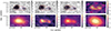 |
Fig. 1. HZ10 HST, ALMA Band 9, 8, and 7, [CII], and Band 6 morphologies in cutouts of 1.3′′ × 2.2′′. Panels A, B, and C contain the WFC3 F105W, F125W, and F160W images, respectively, in grey scale. The black contours in the three panels are the [0.9, 1.2, 2.1] × 10−21 erg s−1 cm−2 Å−1 levels of the F105W, F125W, and F160W filters. The blue-dashed and red-solid contours correspond to [3σ, 4σ, 5σ] and [6σ, 12σ, 18σ] levels for the 77 μm continuum and [CII] integrated intensity, respectively. From D to H: Panels include the 77 μm ALMA continuum, 110 μm ALMA continuum, 158 μm ALMA continuum, and 158 μm [CII], and 198 μm ALMA continuum images, respectively. Contours levels in panels D and G are the same as in panel A, B, and C, for 77 μm continuum, and [CII] integrated intensity, respectively. While blue-solid contours in panels E and H [3σ, 4σ, 5σ] levels for 110 μm and 198 μm ALMA continuum maps, respectively, the white-solid contours in panel G are the [6σ, 4σ, 5σ] levels for the 158 μm ALMA continuum maps. Finally, while green crosses in panel B are the centers of the Seérsic profiles computed for the three sources (e.g., HZ10-C, HZ10-W, and “the bridge”) analysed in this work (see Sect. 3.2), the green circles correspond to the apertures used to perform the angular resolved analysis (see Sect. 4.2 for more details). |
HZ10 was included in the CRISTAL sample as part of one of the CRISTAL pilot programs that resulted as a combination of the ALMA programs 2019.1.01075.S (P.I.: M. Aravena), and 2012.1.00523.S (P.I.: P. Capak; see Capak et al. 2015 for more details); however, the latter was not considered in this work due to its coarser angular resolution compared to the former. The details of the data reduction of the Band 7 observations are presented in Solimano et al. (2024); among the main features their data processing, the self-calibrated and combined measurement sets were processed with CRISTAL’s reduction pipeline as described in Herrera-Camus et al. (in prep.). Briefly, it starts by subtracting the continuum on the visibility space using the Common Astronomy Software Application (CASA; CASA Team 2022) uvcontsub task. Afterward, it runs tclean with automasking multiple times, producing cubes with different weightings and channel widths. In all cases, the data were cleaned down to 1σ. In this work, we used datacubes with a 20 km s−1 channel width and Briggs (robust=0.5) weighting. The ancillary ALMA Band 8 and Band 6 observations are presented in Faisst et al. (2020), using Briggs weighting (Briggs 1995) for the image reconstruction, with a robust = 0.5.
In addition, we included HST data for HZ10 as part of project 13641 (P.I.: Peter Capak), retrieved from the Barbara A. Mikulski Archive for Space Telescopes (MAST1). The data comprise Wide Field Camera 3 images (WFC3), including the F105W (panel A in Fig. 1), F125W, and F160W bands. These bands cover a rest-frame wavelength range between ∼1200 to 2200 Å.
3. Methods and products
3.1. Basic equations and assumptions
To compute the integrated [CII] line emission and the rest-frame 77 μm, 110 μm, 158 μm, and 198 μm continuum fluxes, we use the following equation:
 (1)
(1)
where A is the area of a circular aperture with a diameter equivalent to the major axis of the 198 μm continuum beamsize (i.e., the coarsest angular resolution among the full dataset;  ) and centered at the position of the bridge (see Sect. 4.2 for more details). Here, Ii is the velocity integrated flux density (in Jy km/s beam−1) for [CII], and flux density (in Jy beam−1) for dust-continuum bands. Finally, i= [CII], 77 μm, 110 μm, 158 μm, and 198 μm.
We also used Eq. (1) to compute resolved values for the three components of HZ10 identified in this work. In this case, A is the area of a circular aperture with a diameter equal to the major axis of the 77 μm continuum beamsize (i.e., the coarser angular resolution between ALMA Band 7 and 9 data;  ) and centered at the locations of the three components identified in HZ10 (green circles in panels B and D from Fig. 1).
We used the SED parametrization from Casey (2012) to compute the best spectral energy distribution (SED) fitting, which corresponds to:
 (2)
(2)
with
 (3)
(3)
where Nbb is the normalization, βd is the emissivity index, TSED is the SED dust temperature, λ0 is the wavelength at optical depth τ = 1, λc is the power-law turnover wavelength, and c is the speed of light. We used λ0 = 100 μm for the global and resolved HZ10 SED fittings, as applied in Faisst et al. (2020). From Casey (2012), we also adopt the parametrization of  , where L(α, TSED)=[(b1 + b2α)−2 + (b3 + b4α)×TSED]−1 (with b1 = 26.68, b2 = 6.246, b3 = 1.905 × 10⁻⁴, and b4 = 7.243 × 10⁻⁵, and where α = 2.0; see Casey 2012 for more details). We note that upcoming CRISTAL papers (e.g., Li et al. 2024) will use other SED fitting methodologies (e.g., SED fitting codes based on the implementation of energy balances such as MAGPHYS; da Cunha et al. 2008) to provide independent estimations of both dust temperature and its related physical quantities.
We compute the peak dust temperature (Tpeak; e.g. Béthermin et al. 2015; Schreiber et al. 2018), which is derived from the IR emission by the Wien’s displacement law,
 (4)
(4)
Since the contribution from background CMB heating could potentially affect dust temperatures at z > 5 (e.g., da Cunha et al. 2013; Faisst et al. 2020), we apply CMB corrections to our TSED estimations using Equation (12) from da Cunha et al. (2013):
![Mathematical equation: $$ \begin{aligned} T_{\rm dust}(z) = [(T^{z=0}_{\rm dust})^{4+\beta _{\rm d}} + (T^{z=0}_{\rm CMB})^{4+\beta _{\rm d}} ([1+z]^{4+\beta _{\rm d}}-1) ]^{\frac{1}{4+\beta _{\rm d}}}, \end{aligned} $$](/articles/aa/full_html/2024/11/aa51490-24/aa51490-24-eq15.gif) (5)
(5)
where  and
and  are the dust temperature and the CMB temperature measured at z = 0, respectively. Throughout this paper, we have adopted
  K.
K.
To compute the total FIR luminosity (LFIR), we perform a numerical integration of Eq. (2) in the wavelength range between 42.5 and 125.5 μm (e.g., Helou et al. 1988). To do so, we adopt the best-SED fitting parameters of the source (see Sect. 4.2 for more details), and we compute the total FIR luminosity, LFIR, by integrating the flux between 42.5 and 122.5 μm (as described in Faisst et al. 2020). Similarly, we also compute the total IR luminosity (LIR) by integrating numerically the best-fitting SED but in the wavelength range between 8 and 1000 μm.
We obtain the [CII] luminosity (in K km s−1 pc2) using the following equation (Solomon & Vanden Bout 2005):
![Mathematical equation: $$ \begin{aligned} L_{\rm [CII]} = 3.25 \times 10^7 S_{\rm {CII}} \Delta v \, \nu ^{-2}_{\rm obs} \, D^{2}_{\rm L} \, (1+z)^{-3}, \end{aligned} $$](/articles/aa/full_html/2024/11/aa51490-24/aa51490-24-eq19.gif) (6)
(6)
where SCIIΔv is the velocity integrated flux (in Jy km/s beam−1),  is the luminosity distance (in Mpc), νobs is the observed frequency (in GHz), and z is the redshift.
The UV spectral slope (βUV) is derived from HST WFC3 F125W and F160W images and using Equation (1) in Liang et al. (2021):
 (7)
(7)
where fλ, 0.19 and fλ, 0.23 are the specific fluxes at 1877 Å and 2311 Å rest frame taken from the F125W and F160W images, respectively. We compute βUV by taking advantage of its almost constant value along the wavelength range 1260 < λ < 3200 Å, avoiding contamination by the 2175 Å “bump” feature.
Finally, we compute the IR excess (IRX) using the equation (e.g., Meurer et al. 1999; Popping et al. 2017)
 (8)
(8)
where LUV is the monochromatic rest-frame UV luminosity at  . To derive L1600 Å, we used the HST WFC3/F105W image (see panel A in Fig. 1) and the PHOTFLAM constant to convert the flux from e−/s to erg s−1/cm2/Å.
3.2. Parametric 2D fitting
As Fig. 1 shows, the ALMA Band 9 and 7 high angular resolution observations reveal that HZ10 is a complex system with (at least) two main components: a central one (HZ10-C) and one in the westward direction (HZ10-W). To derive the morphological parameters of these two components, we used the 2D light profile modeling code PYAUTOGALAXY2 (Nightingale et al. 2023), which is based on PYAUTOFIT (Nightingale et al. 2021). Implementing the image-based filter PYAUTOGALAXY mode for a faster workflow, we generate the noise-map by feeding the full covariance matrix into the calculation of the likelihood using the code ESSENCE3 (Tsukui et al. 2023). We modeled the HZ10-C and HZ10-W morphologies by fitting a single 2D Sérsic profile (Sersic 1968), with a total of seven free parameters: the coordinates of the source’s center (RA and Dec), the coordinate of the vector of the Sérsic profile’s minor and major axes (x, y), the effective radius (Re), the Sérsic’s index (n), and the intensity at the center (I0[r = 0]).
We performed three independent fits to derive the morphologies of the rest-frame 77 μm continuum (Band 9) and the 158 μm continuum and [CII] line emission maps (Band 7). While the continuum maps are directly generated after running the tclean task in CASA, we produced the [CII] intensity map (or moment 0 maps) by fitting a Gaussian function to the line profile and integrating the emission in the spectral range [μ-FWTM, μ+FWTM] (where μ is the central frequency and FWTM is the full width at one-tenth of maximum of the Gaussian profile). We used the following method to compute the best morphological parameters of the emission:
-
1.
We estimated the centroid using 2D Gaussian functions (RA and Dec) of the 77 μm continuum emission of HZ10-C and HZ10-W. We used these coordinates as an initial guess to look for the centers of the two 2D Sérsic profiles.
-
2.
Then, we used the task minimize from the PYTHON package lmfit (Newville et al. 2015). We performed a two-step best-parameter search: we adopted the least_squares method, followed by the emcee method (the latter looks for the maximum likelihood via a Markov chain Monte Carlo algorithm). To do so, we constrained the values of n and I0 within the ranges [0.1, 3] and [0, 2Imax], respectively (Imax is the maximum value of the intensity map).
-
3.
Finally, we repeated step 2 for the 158 μm continuum and the [CII] line emission maps, this time using the 77 μm continuum best parameters as a prior (i.e., centroids, Sérsic indexes, Imax).
Table 2 lists the best parameters and uncertainties of the fitting procedure. We note that the differences in DEC in Table 2 are larger than the spatial resolutions of the observations in each band (see Sect. 2.2).
Results of the parametric 2D fitting.
4. Results and discussion
4.1. Structure of HZ10
Figure 2 shows the results of the 2D parametric fitting, confirming the complex structure of HZ10. The figure shows this system has (at least) two main components, HZ10-C and HZ10-W, each of them slightly showing different morphologies depending on the datasets. On the one hand, HZ10-W shows a slightly more extended distribution of the [CII] emission than HZ10-C; on the other hand, the two components have surprisingly similar Sérsic profiles when analyzing the 77 and 158 μm continuum maps. These results may reflect significant dust content (relative to the gas) in HZ10-W that causes severe dust attenuation, as evidenced by its faint UV emission (shown in panel A of Fig. 1).
 |
Fig. 2. Results from the parametric 2D modeling of HZ10 using PYAUTOGALAXY, in panels of 3′′ × 3′′. While the left panels contain the observed emission (colormap and black-solid contours), the middle and right panels show the best model using 2D Sérsic profiles (see Table 2 for more details) and the residuals after subtracting the maximum likelihood model, respectively. From top to bottom, panels contain the rest-frame 77 μm ALMA continuum (top row), 158 μm ALMA continuum (middle row), and [CII] 158 μm line emission (top row). The beam sizes of the data are represented by ellipses at the bottom-left of middle panels. For all the subplots, the contour are the [0 (dashed), 4σ, 5σ, and 6σ] levels. The figure confirms the binary nature of HZ10, which can be decomposed in HZ10-C (at the center), HZ10-W (to the left), and the bridge between the two main components (with at least a 5σ significance on the residual 158 μm continuum map). The latter seems to reflect the extended dusty component connecting HZ10-C and HZ10-W. |
Interestingly, the middle row of Fig. 2 shows that the HZ10 system cannot be described just considering two Sérsic profiles. A visual inspection of the residual map of the 158 μm continuum emission reveals a third component connecting HZ10-C with HZ10-W. When applying the procedure described in Sect. 3.2 to the residual 158 μm map, we note that the extra component (or the bridge) cannot be well described by a Sérsic profile (after trying to fit a Sérsic profile to the residuals). To analyze the physical properties of the dust at the bridge, we derived the coordinates of the centroid of its 158 μm continuum emission (RAInt, Dec.Int); we obtain (10h00m59 279 ± 0
 037, +01
 038).
038).
The presence of the bridge may suggest that there is possibly an interaction or a tidal tale connecting the two main components of the HZ10 system. We are in the process of conducting a more detailed analysis of the [CII] morphology to further probe the interacting nature of the system to be published in a forthcoming paper (Telikova et al., in prep.). This third component is also presented in new and deep JWST/NIRSpec IFU observations of the main nebular lines in HZ10 (Jones et al. 2024).
4.2. SED fitting, TSED and Tpeak
We performed a FIR SED fitting in order to determine the physical conditions of the dust in HZ10. We used Eq. (1) to compute the global values of the 77 μm, 110 μm, 158 μm, and 198 μm dust-continuum fluxes, which correspond to the sum of all the flux within a circular area with a diameter equivalent to the major axis of the 198 μm continuum beamsize. We recall that the latter is the coarsest angular resolution among all the dataset (i.e.,  kpc at HZ10’s distance). The aperture was placed at the 158 μm continuum emission centroid of the bridge (see Sect. 4.1). To do this, we convolved all the maps to the coarsest angular resolution among the continuum maps (i.e., 198 μm dust-continuum beamsize). We then used these fluxes to look for the best-fit parameters of Eqs. (2) and (3) by performing the task minimize from the PYTHON package lmfit (Newville et al. 2016). We adopted the emcee method, which determines the maximum likelihood of the parameters via a Markov chain Monte-Carlo (MCMC). Finally, we chose fixed values for α = 2.0 and λ0 = 100 μm to perform the fitting (see Sect. 3.1). The results, including the best parameters for the FIR SED fitting and the 1σ uncertainties curves, are shown in Fig. 3. We highlight that the ALMA Band 9 data, which are closer to the SED peak of HZ10 (see Fig. 4), allow us to reduce the uncertainties by almost three times those of the TSED estimations, when compared to global estimations included in previous studies (e.g., Faisst et al. 2020; Mitsuhashi et al. 2024b).
 |
Fig. 3. Best-fitting IR SEDs for the global ALMA Bands 9, 8, 7, and 6 continuum emission of HZ10 (77 μm, 110 μm, 158 μm, and 198 μm, respectively). The wavelength is given in the rest frame. The blue-solid line corresponds to the best-modified SED given by Eqs. (2)–(4) and using the maximum likelihood parameters (see top-left corner). The combination between new ALMA Band 9 and 7 continuum measurements (77 μm and 158 μm rest frame, respectively) allows us to probe the peak of the dust SED, and hence constrain these parameters accurately. In addition, we have included estimations of the global continuum emission flux for HZ10 from Capak et al. (2015) (orange square) and Faisst et al. (2020) (green triangles) to contrast our estimations with previous results. |
 |
Fig. 4. Best-fitting results for FIR SEDs for 77 and 158 μm continuum emission, using Eqs. (2)–(3) and adopting the βd obtained in Fig. 3, for the three components identified in the analysis from Sect. 4.1: HZ10-C (left panel), HZ10-W (middle panel), and the bridge (right panel). Conventions are the same as in Fig. 3. As shown in Figs. 1 and 2, HZ10-C and the bridge have lower 77 μm continuum emission, compared to that for HZ10-W (although still within the uncertainties); this may be reflecting a strong UV dust absorption in HZ10-W, which translates into a higher TSED temperature when compared to those of the other two components (although all of them with the same temperature within 1σ). |
We also perform the FIR SED fitting for the three sources described in Sect. 4.1. Similarly to way than for the global SED fitting described above, we used a circular aperture with a diameter equivalent to the major axis of the 77 μm continuum (i.e., the coarsest angular resolution among the [CII] line, 77, and 158 μm continuum emission maps;  , or ∼2.5 kpc) to compute the integrated fluxes within such an aperture (included in Table 3). The aperture is located at three different positions given by the centers of the 77 μm continuum Sérsic profiles for HZ10-C and HZ10-W (see Table 2), and the 158 μm continuum emission centroid of the bridge. The integrated fluxes are shown in Table 3.
Main properties of the HZ10 system derived in this work.
When comparing our results from the integrated SED fitting with previous studies, we found a dust emissivity index of βd = 2.00 ± 0.14, which is slightly lower (although still consistent) than that derived from Faisst et al. (2020) ( ; based on the SED modelling of Band 6, 7 and 8 data). Conversely, our estimated global SED dust temperature is statistically identical to the one derived by Faisst et al. (2020) to ours (
 and 46.7 ± 6.8 K, respectively). We remark that βd, TSED, and Tpeak (derived from Eq. (4)) are very sensitive to both the assumptions for the fixed values and the completeness of the dust-continuum dataset.
For the resolved SED FIR SED fitting, and considering the caveat above, we adopted a fixed value for βd = 2.0 (i.e., the value derived from the global SED fitting). We found slight differences n the Tdust estimations when compared to the integrated quantities included in Faisst et al. (2020). Our results of the FIR SED fitting for the three components, including the best parameters and the 1σ uncertainty curves, are shown in Fig. 4. Although still within the uncertainties, we note that the resolved structure of the dust revealed by the data presented in this work shows that the TSED depends critically on the component of the HZ10 system.
While the SED dust temperature in HZ10-C is consistent with integrated values presented by previous studies (46.4 K), we note that HZ10-W’s TSED is found to be ∼5 K higher, although statistically insignificant (less than 1σ), than that of the central component and previous global estimations by Faisst et al. (2020) (51.2 and 46.2 K, respectively). Interestingly, we also find that the bridge has a lower TSED values (although still consistent; 39.2±9.8) compared to HZ10-C and HZ10-W. The latter seems to be reflecting the detached nature of the bridge respect to the two main components (perhaps due to outflows), without the close sources of hard radiation fields that would be required to increase its Tdust up to temperatures similar to those of HZ10-C and HZ10-W.
To put the results from HZ10 in a more general context, Fig. 5 shows the evolution of peak dust temperature in star-forming galaxies (expected evolution of the peak temperature derived from Eq. (4), Tpeak) as a function of redshift. The combination of Tpeak measurements for low-z galaxies and the interpolation of these estimations at high redshift suggests that temperatures increase up to z ∼ 4 and then flatten off following hydrodynamical simulations from Liang et al. (2019) (blue dashed-dotted line in Fig. 5). The scatter from the linear relation expected for galaxies at 0.5 < z < 4 (see black-dashed line in Fig. 5) has been shown to depend on many factors. Some of them have been identified in galaxies from the local Universe (e.g., KINGFISH; Skibba et al. 2011, GOALS; U et al. 2012), including changes in the dust mass density, effects on the dust opacity, and/or variability in the UV luminosity of a central source (e.g., young stars or AGN activity). For instance, Faisst et al. (2017) proposed that metallicity also has a significant effect on the Tpeak measured. In particular, their results indicate that galaxies with faint IR emission and low metallicity could have Tpeak values similar to those for high IR luminous galaxies. In addition, metallicity can potentially alter the dust properties (e.g., Pak et al. 1998; Misselt et al. 1999; Sommovigo et al. 2022), mainly producing environments with lower opacities (e.g., Issa et al. 1990; Lisenfeld & Ferrara 1998). This is due to the fact that harder stellar radiation fields are expected for low-metallicity environments, the dust temperature is altered.
 |
Fig. 5. Peak dust temperature (Tpeak) evolution with redshift for HZ10-C, HZ10-W, and the bridge as blue, orange, and green squares, respectively. The figure also includes galaxy samples at different redshift ranges: z = 0.2 − 4 (gray unfilled circles from ALESS; da Cunha et al. 2015; yellow triangles, Béthermin et al. 2015; the two latter samples are shown as included in Fig. 6 from Faisst et al. 2020), and z > 6 (purple circles; Knudsen et al. 2016; Hashimoto et al. 2019; turquoise pentagons, Algera et al. 2024). The red triangle, black circle, and brown circle are galaxies at z ∼ 5 included in Faisst et al. (2020). Magenta stars correspond to z ∼ 7 galaxies selected from the Reionization Era Bright Emission Line Survey, REBELS (Sommovigo et al. 2022). Blue large dark-blue circles correspond to galaxies from at 0.5 < z < 4 selected from the deep CANDELS fields, and the dashed-black line correspond to their linear best-fit, both extracted from Schreiber et al. (2018). Green inverted triangles correspond to results based on the stacking analysis and the expected redshift evolution from Viero et al. (2022). The blue dot-dashed line is the expected peak temperature evolution from hydrodynamic simulation (Liang et al. 2019; Ma et al. 2019). Red unfilled circles correspond to galaxies at z ≳ 6 selected from the Systematic Exploration in the Reionization Epoch using Nebular And Dust Emission (SERENADE; Harikane et al., in prep.), as included in Mitsuhashi et al. (2024a). The sample also contains three galaxies selected from Harikane et al. (2020). Finally, red and green dashed areas are correspond to the parameter space covered by galaxies selected at different redshfits from the Herschel Multi-tiered Extragalactic Survey (HerMES; Magnelli et al. 2014) and ultraluminous infrared galaxies selected from the Great Observatories All-sky LIRG Survey (GOALS; U et al. 2012), respectively. |
Based on the HST WFC3/F160W data of HZ10-W shown in panel A of Figure 1, the higher TSED may be responding to UV emission severely attenuated by dust, producing a significant increase of the dust temperature. Spectroscopic observations of the main nebular lines with JWST/NIRSpec (e.g., Jones et al. 2024) and future ALMA Band 10 continuum and JWST observations could help us to get better constraints on the dust emission and metallicity, thus allowing us to break down the potential degeneracy of the TSED estimations.
4.3. The physical properties of the ISM in HZ10
Figure 6 presents the relation between FIR luminosity, LFIR, and TSED for the three components of HZ10 identified in this work. The values of LFIR for HZ10-C, HZ10-W, and the bridge are consistent with the global FIR luminosity derived by Faisst et al. (2020). However, compared to the expected relation from the optically thick case (i.e., where L ∝ T4; grey-dashed line in Fig. 6), the HZ10 components seem to be either too warm (i.e., to the right of the relation) or underluminous in the FIR (thus, below the relation). In addition, when compared to dusty star-forming galaxies at similar redshifts (DSFG, included as gray solid circles in Fig. 6; Riechers et al. 2020), our LFIR values may be reflecting intrinsic differences of the dust properties between some CRISTAL and DSFG systems, but most likely due different spatial configuration and/or optically thickness. Some of these differences could respond as well to the factors described at the end of Sect. 4.2, including the effects of metallicity, dust abundance on the dust opacity (Faisst et al. 2017), or changes in the photoelectric efficiency of the dust (e.g., Nath et al. 1999; Malhotra et al. 2017; McKinney et al. 2021; Glatzle et al. 2022).
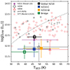 |
Fig. 6. Comparison of FIR luminosity (LFIR) and SED temperatures (TSED) for the three components of HZ10 covered in this work. The figure includes a sample of dust star-forming galaxies at z > 5 (gray solid circles; Riechers et al. 2020), which are dusty star-forming galaxies with strong gravitational lensing, at 1.9 < z < 6.9. These galaxies were included in Reuter et al. (2020), along with previous comparisons for HZ09 (black unfilled circle), HZ04 (red empty triangle), and HZ10 (purple filled circle), as in Faisst et al. (2020). The gray dashed line is the L ∝ T4 relation, also taken from Faisst et al. (2020). |
The [CII]-to-FIR luminosity ratio, [CII]/FIR = L[CII]/LFIR, has been found to be closely related to the physical properties of the ISM. For instance, while in low-metallicity environments, the typical values are log([CII]/FIR) ∼ −2 (e.g., dwarf galaxies or star-forming disks; Madden et al. 2013; Smith et al. 2017; Herrera-Camus et al. 2018a), in nuclear regions, starburst systems, and AGNs are around log([CII]/FIR) ∼ [−4, −3] (e.g., Malhotra et al. 2001; Díaz-Santos et al. 2013; Herrera-Camus et al. 2018a).
Figure 7 shows [C II]/FIR as a function of the FIR luminosity surface density, ΣFIR, for the three components of HZ10 analyzed in this work. We note that HZ10-C, HZ10-W, and the bridge have a very smooth distribution of [CII]-to-FIR values, with a variation at most as 25% between the faintest (i.e., the bridge) and the strongest continuum emission (i.e., HZ10-W). Although differences in the [CII] emission are slightly more significant, these are at 35–45% between the faintest (i.e., the bridge and HZ10-W) and the strongest [CII] emitter (HZ10-C). Our results are consistent with those of ∼100 pc scale regions in the central disk of the nearby starburst galaxy M82 (green unfilled dots; Contursi et al. 2013; Herrera-Camus et al. 2018a). Following a similar methodology to that described in Sect. 4.2 to the physical parameters of the dust in a typical star-forming galaxy at z ∼ 5.5 (βd = 1.5, TSED = 45 K; e.g., Pavesi et al. 2016; Faisst et al. 2017), Herrera-Camus et al. (2021) compute the [CII]/FIR-ΣFIR relation for HZ04 (CRISTAL-20 in the CRISTAL survey). Splitting the analysis in four independent beams (red unfilled triangles in Fig. 7), they find log([CII]/FIR) ∼ [ − 2.7, −2.3] and log(ΣFIR/[L⊙ kpc−2]) ∼ 10. Although [CII]/FIR values for our sources are comparable to those for HZ04, we note that our sources have ΣFIR values (i.e., the star formation rate, SFR) around four times higher than those derived in Herrera-Camus et al. (2021). These results may suggest a deficit in the [CII] content in the HZ10 system, specially in HZ10-W; however, we note that the dust SED setup used in Herrera-Camus et al. (2021) is different to ours and therefore this may affect the comparison between the two sources given its impact on the derived IR luminosities.
 |
Fig. 7. [CII] /FIR ratio as a function of the FIR surface density (ΣFIR) for HZ10-C (blue square), HZ10-W (orange square), and the bridge between them (green empty square). For comparison, the figure also includes nearby star-forming and starburst galaxies from the SHINING sample (grey filled stars; Herrera-Camus et al. 2018a), ∼100 pc scale regions in the central disk of M82 (green unfilled dots; Contursi et al. 2013; Herrera-Camus et al. 2018a), ∼400 pc scale regions from central regions of M83 (purple filled circles), lensed dusty star-forming galaxies at z ∼ 1.9 − 5.7 (DSFGs; red-solid diamonds; Spilker et al. 2016), and four kpc-size regions extracted across the disk of HZ04 (red unfilled triangles; Herrera-Camus et al. 2021). The solid grey line corresponds to the best quadratic fit to the SHINING data (as included in Herrera-Camus et al. 2018a). |
Several studies have shown the strong impact that AGNs could potentially have on the [CII] line emission, producing low [CII]-to-FIR luminosity ratios in nearby galaxies (e.g., Stacey et al. 2010; Sargsyan et al. 2012; Herrera-Camus et al. 2018b). Díaz-Santos et al. (2013) suggest that in galaxies with a strong [CII] deficit (log([CII]/FIR) < −3) the AGNs can play an important role in destroying significant fractions of polycyclic aromatic hydrocarbon (PAH) molecules (i.e., associated with [CII] emission) due to their hard radiation field (e.g., Lai et al. 2023). This is consistent with the evidence (although marginal) from the new JWST/NIRSpec observations that suggest that HZ10-W may contain nuclear activity (Jones et al. 2024). On the other hand, by modeling the emission of the molecular, neutral, and ionized gas of galaxies selected from the Survey with Herschel of the Interstellar medium in INfrared Galaxies (SHINING), Graciá-Carpio et al. (2011) found that a decrease in [CII]/FIR ratios can be explained by increasing the value of the ionization parameter (U) on the surface of molecular clouds. As U increases, a larger fraction of UV photons are absorbed by dust in the ionized region and reemitted in the form of infrared emission. The net effect is that the fraction of UV photons available to ionize and excite the gas is reduced at high U, decreasing the relative intensity of the fine structure lines compared to the FIR continuum (e.g, Voit 1992; Abel et al. 2009; Graciá-Carpio et al. 2011; Herrera-Camus et al. 2018a). However, the UV photons could be also interacting with gas itself, having a potential impact on its physical properties (i.e., the [CII] line emission).
4.4. The IRX-βUV relation
Unbiased galaxy star-formation rates at low and high redshift are essential to get a complete picture of the mechanisms changing the physical properties of the ISM as a function of cosmic times. It is critical thus to account for both the dust thermal emission and the UV light to mitigate the natural biases on the derivation of accurate SFR estimations. In this sense, the IRX-βUV relation (e.g., Meurer et al. 1995, 1999) has shown to be a strong observational tool to link the IR emission to UV measurements, particularly to the tight correlations of the IRX-βUV plane exhibited at different redshift ranges (e.g., Heinis et al. 2013; McLure et al. 2018; Fudamoto et al. 2020; Bowler et al. 2024). In recent decades, however, several studies have revealed that some local LIRGs/ULIRGs (e.g., Howell et al. 2010) and high-z galaxies (e.g., Álvarez-Márquez et al. 2016; Bouwens et al. 2016; Reddy et al. 2018) can depart from this relation due to changes in intrinsic dust properties. Such variations can be produced by the composition of the dust or the spatial distribution of the dust and UV emission; alternatively, they may be due to ISM turbulence, among other effects (see Liang et al. 2021 and references therein).
To find the more adequate scenario in the HZ10 system, we used Eqs. (7) and (8) to drawn the IRX-βUV relation for HZ10-C, HZ10-W, and the bridge, as shown in Fig. 8. In addition to several galaxy samples at different redshifts, we have also overplotted some of the schematics from Fig. 11 in Popping et al. (2017), which reflect the distinct physical mechanisms affecting the properties of the emission sources (see light-blue and light-orange shaded areas, along with the green arrow at the bottom of Fig. 8). While HZ10-C is close to the best linear-fit for UV-selected near starburst galaxies (black solid line; Meurer et al. 1999), we note that both HZ10-W and the bridge lie significantly above it; the former also has significantly a higher βUV value compared to that for the other two members (βUV ≈ −0.64), which is consistent with the results included in Jones et al. (2024). According to Popping et al. (2017) models, the location of HZ10-W and the bridge in the IRX-βUV relation seems to favor scenarios where a screen of dust is placed with holes in between a relative young stellar population and the observer. Although a small level of turbulence within the dust could also increase its optical depth (e.g., Fischera et al. 2003; Popping et al. 2017), the dust screen appears to be a simple (yet reasonable) explanation for the dust emission in the “dustier” components of the HZ10 system. For example, although with higher βUV than those for the three components analyzed in this work, the star-forming main sequence galaxies analyzed by Fudamoto et al. (2020) have similar IRX values than HZ10’s. They propose that the high dust-attenuation properties shown by those galaxies may correspond to supernovae (SNe) driven dust production at z ≥ 2 − 3. Such SNe dust could be consistent with the steeper dust curve observed at z ∼ 4 − 6 galaxy sample compared to the attenuation inferred at z < 3 for sources similar to those included in Meurer et al. (1999) (e.g., Maiolino et al. 2004; Hirashita et al. 2005; Gallerani et al. 2010).
 |
Fig. 8. Comparison between the IR excess (IRX) and the UV spectral slope (βUV); i.e., the IRX-βUV relation for HZ10-C, HZ10-W, and the bridge between them. The conventions are as in Fig. 7. Green diamonds correspond to the MASSIVEFIRE sample at z = 6, as included in Liang et al. (2021). The figure also encompasses a series of galaxy samples from the literature: yellow triangles are taken from Heinis et al. (2013), red stars from Álvarez-Márquez et al. (2016), orange stars from Bouwens et al. (2016), blue-edge diamonds from Reddy et al. (2018), magenta-edged circles from McLure et al. (2018), and cyan-edged squares from Fudamoto et al. (2020). The black solid line is the best linear-fit for the IRX-βUV relation for UV-selected starburst galaxies as shown in Meurer et al. (1999). The light-blue and light-orange shaded areas, as well as the green arrow at the bottom are extracted from the schematic figure included in Popping et al. (2017), which summarizes the different physical mechanisms affecting the properties of the emission sources. |
Numerical simulations have also revealed that [CII]/FIR ratios can decrease with increasing ΣFIR, leading to an apparent [CII] deficit. In particular, Bisbas et al. (2022) show that this could reflect the thermal saturation of [CII] as a consequence of the strong far-UV heating related to the high SFR. These authors proposed that while the [CII] emissivity increase asymptotically in this regime, the FIR emission increases linearly, leading the deficit in the [CII].
The IRX-βUV relation has been shown to be a powerful tool to characterize the complex structure of the HZ10 system. However, some studies have suggested the that IRX-βUV relation may fail in terms of probing the physical conditions of the ISM in galaxies with large IR-to-UV flux ratios compared to the βUV (e.g., Ferrara et al. 2022). To address this problem, Ferrara et al. (2022) introduce the non-dimensional “molecular index”, Im=(F158 μm/F1500Å)/(βUV−βint). Here, F158 μm and F1500 Å are the fluxes at 1500 Å and the observed far-infrared continuum flux at 158 μm, respectively, and βint is the intrinsic UV spectral slope (typically, βint ≈ −2.406; see Ferrara et al. 2022 for more details). When applied to sources selected from REBELS, they noted that Im is a good predictor of the simultaneous presence of optically thin and thick regimes, showing that galaxies with a two-phase medium have Im > 1120. When computing the molecular index for the HZ10 system, we obtained Im = 1156 ± 104. The latter is consistent with the IRX-βUV relation for HZ10 discussed above, supporting the scenario of a two-phase structure with young stars embedded in optically thick giant molecular clouds and an older stellar populations immersed in a more transparent medium.
Future ALMA-CRISTAL studies (Killi et al., in prep.) will analyze the variations of the IRX-βUV relation among CRISTAL galaxies on ∼kiloparsec scales. This will allow us to derive more statistically significant results and perform a meticulous comparison with other similar studies from the literature.
5. Summary and conclusions
We present a study of the dusty, main-sequence galaxy HZ10 at z ≈ 5.66, as part of the CRISTAL survey. We present new ALMA [CII] line emission and Band 9 dust continuum data, which is key to constrain the peak of the dust SED. In combination with ALMA Band 6, 7, 8, and HST WFC3 archival data, we conducted a systematic analysis of the morphology and the physical conditions of dust and gas in such multi-component system. We characterize the main properties of the structures identified in HZ10, such as the SED and peak dust temperatures, FIR luminosities, [CII]/FIR ratios, UV spectral slopes, and their IR excesses. We compare our results with the current literature. We present our main conclusions below.
-
We performed a parametric 2D fitting to derive the morphological parameters of the two main components of HZ10 (HZ10-C and HZ10-W), which are well described by Sérsic profiles in the 77 and 158 μm dust continuum and the [CII] line emission data (see Table 2). Interestingly, the residual map of the 158 μm dust continuum data reveals a third component (bridge), which seems to correspond to a bridge-like dusty structure connecting the central and west components.
-
We carried out a global modified blackbody SED fitting of HZ10 using the 77, 110, 158, and 198 μm dust continuum fluxes. We derive a global dust emissivity index βd ≈ 2.0 ± 0.14 and a global dust temperature of TSED = 46.7 ± 6.8 K. We adopt the global value of βd to perform modified SED fittings of the three main structures identified in the HZ10 system using the 77 and 158 μm dust continuum maps (since these two datasets allow us to resolve spatially the three components of HZ10), obtaining spatially-resolved estimations of their SED and peak dust temperatures. We find that HZ10-W, which is the component that shows the higher obscuration of the rest-frame UV emission, has a dust temperature of TSED = 51.2 ± 13.1 K, which is about ∼5 K higher than the two other components (although all of them with the almost the same SED temperature within 1σ). More importantly, the inclusion of the new ALMA Band 9 continuum data allow us to reduce the uncertainties in the global dust temperature measurements by a factor of ∼2.3.
-
We computed the [CII]-to-FIR luminosity ratio, [CII]/FIR, for HZ10-C, HZ10-W, and the bridge. When we compare [CII]/FIR with the FIR surface density, ΣFIR, we find that our sources cover a similar parameter space to that of local starburst galaxies. We note that HZ10-W shows signs of a [CII] deficit, suggesting a range of plausible scenarios, such as the hard radiation field destroying PAHs associated with [CII] emission (e.g., young stellar populations or AGN activity) or variations in the dust photoelectric efficiency.
-
We calculated the IR excesses and the UV spectral slopes (the IRX-βUV relation), for the three components in HZ10. While HZ10-C has IRX and βUV values consistent with those of UV-selected starburst local galaxies and other high-z galaxies, both HZ10-W and the bridge clearly depart from the observed sequence of global galaxies the IRX-βUV relation. According to theoretical models from previous studies, our results suggest that the UV-emission in HZ10-W and the bridge may be strongly attenuated by a dust screen in between young stellar populations and the observer.
As mentioned previously, TSED estimations (and related quantities) are very sensitive to the completeness of the integrated FIR continuum fluxes set available to model the dust SED. Complementary continuum fluxes measurements at higher frequencies than those covered by ALMA Band 9 data could thus allow us to get better constraints on the dust temperature of the different components in HZ10. In particular, it is necessary to check possibles scenarios where the dust peak is located at higher frequencies than those covered by Band 9. ALMA Band 10, centered at λBand10 = 350 μm, is a good candidate to address this issue for z ∼ 4 − 6 galaxies. Since it gives spectral coverage in the wavelength range ∼[45, 60] μm at the redshift of HZ10, ALMA Band 10 provides a valuable option for a better characterization of dust continuum emission.
Upcoming ALMA-CRISTAL studies will analyze the [CII], kinematics and morphologies of HZ10, and the variations of the IRX-βUV relation among CRISTAL galaxies in more detail (e.g., Ikeda et al. 2024; Telikova et al., in prep.; Killi et al., in prep.). In addition, future ALMA Band 10 continuum and JWST (e.g., Jones et al. 2024) data will help us obtain better constraints on the dust emission and metallicity of HZ10. This would allow us to break down the potential degeneracy of our dust SED temperature estimations and related physical quantities. In addition, ALMA band 10 data would allow us to trace the small TSED differences and reducing their uncertainties in the HZ10 system.
Acknowledgments
V. V. acknowledges support from the ALMA-ANID Postdoctoral Fellowship under the award ASTRO21-0062. R.H.-C. thanks the Max Planck Society for support under the Partner Group project "The Baryon Cycle in Galaxies" between the Max Planck for Extraterrestrial Physics and the Universidad de Concepción. R.H-C. also gratefully acknowledge financial support from ANID BASAL projects FB210003. R. I. is supported by Grants-in-Aid for Japan Society for the Promotion of Science (JSPS) Fellows (KAKENHI Grant Number 23KJ1006). N.M.F.S. acknowledges financial support from the European Research Council (ERC) Advanced Grant under the European Union’s Horizon Europe research and innovation programme (grant agreement AdG GALPHYS, No. 101055023). K. T. acknowledges support from JSPS KAKENHI grant No. 23K03466. M. K. was supported by the ANID BASAL project FB210003. K. T. was supported by ALMA ANID grant number 31220026 and by the ANID BASAL project FB210003. M. R. acknowledges support from project PID2020-114414GB-100, financed by MCIN/AEI/10.13039/501100011033. M. S. was financially supported by Becas-ANID scolarship #21221511, and also acknowledges ANID BASAL project FB210003. M. A. acknowledges support from FONDECYT grant 1211951, and ANID BASAL project FB210003. R. J. A. was supported by FONDECYT grant number 1231718 and by the ANID BASAL project FB210003. R.B. acknowledges support from an STFC Ernest Rutherford Fellowship [grant number ST/T003596/1]. This paper makes use of the following ALMA data: ADS/JAO.ALMA #2022.1.00678.S, ADS/JAO.ALMA #2019.1.01075.S, ADS/JAO.ALMA #2018.1.00348.S, ADS/JAO.ALMA #2015.1.00388.S. This research is based on observations made with the NASA/ESA Hubble Space Telescope obtained from the Space Telescope Science Institute, which is operated by the Association of Universities for Research in Astronomy, Inc., under NASA contract NAS 5-26555. These observations are associated with program 13641 (P.I.: Peter Capak). The National Radio Astronomy Observatory is a facility of the National Science Foundation operated under cooperative agreement by Associated Universities, Inc. Software: Astropy (Astropy Collaboration 2018), MatPlotLib (Hunter 2007), NumPy (Harris et al. 2020), PYAUTOGALAXY (Nightingale et al. 2023), SciPy (Virtanen et al. 2020), seaborn (Waskom 2021), Scikit-learn (Pedregosa et al. 2011).
References
- Abel, N. P., Dudley, C., Fischer, J., Satyapal, S., & van Hoof, P. A. M. 2009, ApJ, 701, 1147 [Google Scholar]
- Akins, H. B., Fujimoto, S., Finlator, K., et al. 2022, ApJ, 934, 64 [NASA ADS] [CrossRef] [Google Scholar]
- Algera, H. S. B., Inami, H., Sommovigo, L., et al. 2024, MNRAS, 527, 6867 [Google Scholar]
- Álvarez-Márquez, J., Burgarella, D., Heinis, S., et al. 2016, A&A, 587, A122 [NASA ADS] [CrossRef] [EDP Sciences] [Google Scholar]
- Astropy Collaboration (Price-Whelan, A. M., et al.) 2018, AJ, 156, 123 [Google Scholar]
- Bakx, T. J. L. C., Sommovigo, L., Carniani, S., et al. 2021, MNRAS, 508, L58 [NASA ADS] [CrossRef] [Google Scholar]
- Béthermin, M., Daddi, E., Magdis, G., et al. 2015, A&A, 573, A113 [Google Scholar]
- Bisbas, T. G., Walch, S., Naab, T., et al. 2022, ApJ, 934, 115 [NASA ADS] [CrossRef] [Google Scholar]
- Bouwens, R. J., Aravena, M., Decarli, R., et al. 2016, ApJ, 833, 72 [NASA ADS] [CrossRef] [Google Scholar]
- Bouwens, R., González-López, J., Aravena, M., et al. 2020, ApJ, 902, 112 [NASA ADS] [CrossRef] [Google Scholar]
- Bowler, R. A. A., Inami, H., Sommovigo, L., et al. 2024, MNRAS, 527, 5808 [Google Scholar]
- Briggs, D. S. 1995, Ph.D. Thesis, New Mexico Institute of Mining and Technology, USA [Google Scholar]
- Brinchmann, J., Charlot, S., White, S. D. M., et al. 2004, MNRAS, 351, 1151 [Google Scholar]
- Cano-Díaz, M., Sánchez, S. F., Zibetti, S., et al. 2016, ApJ, 821, L26 [Google Scholar]
- Capak, P. L., Carilli, C., Jones, G., et al. 2015, Nature, 522, 455 [NASA ADS] [CrossRef] [Google Scholar]
- CASA Team, Bean, B., Bhatnagar, S., et al. 2022, PASP, 134, 114501 [NASA ADS] [CrossRef] [Google Scholar]
- Casey, C. M. 2012, MNRAS, 425, 3094 [Google Scholar]
- Colombo, D., Sanchez, S. F., Bolatto, A. D., et al. 2020, A&A, 644, A97 [EDP Sciences] [Google Scholar]
- Contursi, A., Poglitsch, A., Graciá Carpio, J., et al. 2013, A&A, 549, A118 [NASA ADS] [CrossRef] [EDP Sciences] [Google Scholar]
- da Cunha, E., Charlot, S., & Elbaz, D. 2008, MNRAS, 388, 1595 [Google Scholar]
- da Cunha, E., Groves, B., Walter, F., et al. 2013, ApJ, 766, 13 [Google Scholar]
- da Cunha, E., Walter, F., Smail, I. R., et al. 2015, ApJ, 806, 110 [Google Scholar]
- da Cunha, E., Hodge, J. A., Casey, C. M., et al. 2021, ApJ, 919, 30 [NASA ADS] [CrossRef] [Google Scholar]
- De Looze, I., Cormier, D., Lebouteiller, V., et al. 2014, A&A, 568, A62 [NASA ADS] [CrossRef] [EDP Sciences] [Google Scholar]
- Díaz-Santos, T., Armus, L., Charmandaris, V., et al. 2013, ApJ, 774, 68 [Google Scholar]
- Díaz-Santos, T., Armus, L., Charmandaris, V., et al. 2017, ApJ, 846, 32 [Google Scholar]
- Faisst, A. L., Capak, P. L., Yan, L., et al. 2017, ApJ, 847, 21 [Google Scholar]
- Faisst, A. L., Fudamoto, Y., Oesch, P. A., et al. 2020, MNRAS, 498, 4192 [NASA ADS] [CrossRef] [Google Scholar]
- Ferrara, A., Hirashita, H., Ouchi, M., & Fujimoto, S. 2017, MNRAS, 471, 5018 [NASA ADS] [CrossRef] [Google Scholar]
- Ferrara, A., Sommovigo, L., Dayal, P., et al. 2022, MNRAS, 512, 58 [NASA ADS] [CrossRef] [Google Scholar]
- Fischera, J., Dopita, M. A., & Sutherland, R. S. 2003, ApJ, 599, L21 [NASA ADS] [CrossRef] [Google Scholar]
- Fudamoto, Y., Oesch, P. A., Magnelli, B., et al. 2020, MNRAS, 491, 4724 [Google Scholar]
- Fudamoto, Y., Smit, R., Bowler, R. A. A., et al. 2022, ApJ, 934, 144 [NASA ADS] [CrossRef] [Google Scholar]
- Fujimoto, S., Ouchi, M., Ferrara, A., et al. 2019, ApJ, 887, 107 [Google Scholar]
- Fujimoto, S., Silverman, J. D., Bethermin, M., et al. 2020, ApJ, 900, 1 [Google Scholar]
- Gallerani, S., Maiolino, R., Juarez, Y., et al. 2010, A&A, 523, A85 [NASA ADS] [CrossRef] [EDP Sciences] [Google Scholar]
- Gallerani, S., Pallottini, A., Feruglio, C., et al. 2018, MNRAS, 473, 1909 [Google Scholar]
- Ginolfi, M., Jones, G. C., Béthermin, M., et al. 2020, A&A, 633, A90 [NASA ADS] [CrossRef] [EDP Sciences] [Google Scholar]
- Glatzle, M., Graziani, L., & Ciardi, B. 2022, MNRAS, 510, 1068 [Google Scholar]
- Graciá-Carpio, J., Sturm, E., Hailey-Dunsheath, S., et al. 2011, ApJ, 728, L7 [Google Scholar]
- Harikane, Y., Ouchi, M., Inoue, A. K., et al. 2020, ApJ, 896, 93 [Google Scholar]
- Harris, C. R., Millman, K. J., van der Walt, S. J., et al. 2020, Nature, 585, 357 [NASA ADS] [CrossRef] [Google Scholar]
- Hashimoto, T., Inoue, A. K., Mawatari, K., et al. 2019, PASJ, 71, 71 [Google Scholar]
- Heinis, S., Buat, V., Béthermin, M., et al. 2013, MNRAS, 429, 1113 [Google Scholar]
- Helou, G., Khan, I. R., Malek, L., & Boehmer, L. 1988, ApJS, 68, 151 [NASA ADS] [CrossRef] [Google Scholar]
- Herrera-Camus, R., Bolatto, A. D., Wolfire, M. G., et al. 2015, ApJ, 800, 1 [Google Scholar]
- Herrera-Camus, R., Sturm, E., Graciá-Carpio, J., et al. 2018a, ApJ, 861, 94 [Google Scholar]
- Herrera-Camus, R., Sturm, E., Graciá-Carpio, J., et al. 2018b, ApJ, 861, 95 [Google Scholar]
- Herrera-Camus, R., Förster Schreiber, N., Genzel, R., et al. 2021, A&A, 649, A31 [NASA ADS] [CrossRef] [EDP Sciences] [Google Scholar]
- Hirashita, H., Nozawa, T., Kozasa, T., Ishii, T. T., & Takeuchi, T. T. 2005, MNRAS, 357, 1077 [CrossRef] [Google Scholar]
- Hodge, J. A., & da Cunha, E. 2020, R. Soc. Open Sci., 7, 200556 [NASA ADS] [CrossRef] [Google Scholar]
- Howell, J. H., Armus, L., Mazzarella, J. M., et al. 2010, ApJ, 715, 572 [Google Scholar]
- Hunter, J. D. 2007, Comput. Sci. Eng., 9, 90 [NASA ADS] [CrossRef] [Google Scholar]
- Ikeda, R., Tadaki, K. I., Mitsuhashi, I., et al. 2024, A&A, submitted, [arXiv:2408.03374] [Google Scholar]
- Inami, H., Algera, H. S. B., Schouws, S., et al. 2022, MNRAS, 515, 3126 [NASA ADS] [CrossRef] [Google Scholar]
- Issa, M. R., MacLaren, I., & Wolfendale, A. W. 1990, A&A, 236, 237 [NASA ADS] [Google Scholar]
- Jones, G. C., Bunker, A. J., Telikova, K., et al. 2024, ArXiv e-prints [arXiv:2405.12955] [Google Scholar]
- Knudsen, K. K., Richard, J., Kneib, J.-P., et al. 2016, MNRAS, 462, L6 [NASA ADS] [CrossRef] [Google Scholar]
- Lai, T. S. Y., Armus, L., Bianchin, M., et al. 2023, ApJ, 957, L26 [NASA ADS] [CrossRef] [Google Scholar]
- Le Fèvre, O., Béthermin, M., Faisst, A., et al. 2020, A&A, 643, A1 [Google Scholar]
- Li, J., Da Cunha, E., González-López, J., et al. 2024, ArXiv e-prints [arXiv:2409.10961] [Google Scholar]
- Liang, L., Feldmann, R., Kereš, D., et al. 2019, MNRAS, 489, 1397 [NASA ADS] [CrossRef] [Google Scholar]
- Liang, L., Feldmann, R., Hayward, C. C., et al. 2021, MNRAS, 502, 3210 [NASA ADS] [CrossRef] [Google Scholar]
- Lisenfeld, U., & Ferrara, A. 1998, ApJ, 496, 145 [NASA ADS] [CrossRef] [Google Scholar]
- Lupi, A., Volonteri, M., Decarli, R., et al. 2019, MNRAS, 488, 4004 [NASA ADS] [CrossRef] [Google Scholar]
- Ma, X., Hayward, C. C., Casey, C. M., et al. 2019, MNRAS, 487, 1844 [NASA ADS] [CrossRef] [Google Scholar]
- Madden, S. C., Rémy-Ruyer, A., Galametz, M., et al. 2013, PASP, 125, 600 [NASA ADS] [CrossRef] [Google Scholar]
- Magdis, G. E., Daddi, E., Béthermin, M., et al. 2012, ApJ, 760, 6 [NASA ADS] [CrossRef] [Google Scholar]
- Magnelli, B., Lutz, D., Saintonge, A., et al. 2014, A&A, 561, A86 [NASA ADS] [CrossRef] [EDP Sciences] [Google Scholar]
- Maiolino, R., Schneider, R., Oliva, E., et al. 2004, Nature, 431, 533 [NASA ADS] [CrossRef] [Google Scholar]
- Malhotra, S., Kaufman, M. J., Hollenbach, D., et al. 2001, ApJ, 561, 766 [Google Scholar]
- Malhotra, S., Rhoads, J. E., Finkelstein, K., et al. 2017, ApJ, 835, 110 [NASA ADS] [CrossRef] [Google Scholar]
- McKinney, J., Armus, L., Pope, A., et al. 2021, ApJ, 908, 238 [NASA ADS] [CrossRef] [Google Scholar]
- McLure, R. J., Dunlop, J. S., Cullen, F., et al. 2018, MNRAS, 476, 3991 [Google Scholar]
- Meurer, G. R., Heckman, T. M., Leitherer, C., et al. 1995, AJ, 110, 2665 [NASA ADS] [CrossRef] [Google Scholar]
- Meurer, G. R., Heckman, T. M., & Calzetti, D. 1999, ApJ, 521, 64 [Google Scholar]
- Misselt, K. A., Clayton, G. C., & Gordon, K. D. 1999, ApJ, 515, 128 [NASA ADS] [CrossRef] [Google Scholar]
- Mitsuhashi, I., Harikane, Y., Bauer, F. E., et al. 2024a, ApJ, 971, 161 [NASA ADS] [CrossRef] [Google Scholar]
- Mitsuhashi, I., Tadaki, K. I., Ikeda, R., et al. 2024b, A&A, 690, A197 [NASA ADS] [CrossRef] [EDP Sciences] [Google Scholar]
- Nath, B. B., Sethi, S. K., & Shchekinov, Y. 1999, MNRAS, 303, 1 [NASA ADS] [CrossRef] [Google Scholar]
- Newville, M., Stensitzki, T., Allen, D. B., & Ingargiola, A. 2015, https://doi.org/10.5281/zenodo.11813 [Google Scholar]
- Newville, M., Stensitzki, T., Allen, D. B., et al. 2016, Lmfit: Non-Linear Least-Square Minimization and Curve-Fitting for Python, Astrophysics Source Code Library [record ascl:1606.014] [Google Scholar]
- Nightingale, J., Hayes, R., & Griffiths, M. 2021, J. Open Source Software, 6, 2550 [Google Scholar]
- Nightingale, J. W., Smith, R. J., He, Q., et al. 2023, MNRAS, 521, 3298 [NASA ADS] [CrossRef] [Google Scholar]
- Pak, S., Jaffe, D. T., van Dishoeck, E. F., Johansson, L. E. B., & Booth, R. S. 1998, ApJ, 498, 735 [NASA ADS] [CrossRef] [Google Scholar]
- Pavesi, R., Riechers, D. A., Capak, P. L., et al. 2016, ApJ, 832, 151 [Google Scholar]
- Pedregosa, F., Varoquaux, G., Gramfort, A., et al. 2011, J. Mach. Learn. Res., 12, 2825 [Google Scholar]
- Pizzati, E., Ferrara, A., Pallottini, A., et al. 2020, MNRAS, 495, 160 [Google Scholar]
- Popping, G., Puglisi, A., & Norman, C. A. 2017, MNRAS, 472, 2315 [Google Scholar]
- Posses, A., Aravena, M., González-López, J., et al. 2024, A&A, submitted, [arXiv:2403.03379] [Google Scholar]
- Reddy, N. A., Oesch, P. A., Bouwens, R. J., et al. 2018, ApJ, 853, 56 [NASA ADS] [CrossRef] [Google Scholar]
- Reuter, C., Vieira, J. D., Spilker, J. S., et al. 2020, ApJ, 902, 78 [NASA ADS] [CrossRef] [Google Scholar]
- Riechers, D. A., Hodge, J. A., Pavesi, R., et al. 2020, ApJ, 895, 81 [Google Scholar]
- Saintonge, A., Catinella, B., Cortese, L., et al. 2016, MNRAS, 462, 1749 [Google Scholar]
- Sargsyan, L., Lebouteiller, V., Weedman, D., et al. 2012, ApJ, 755, 171 [Google Scholar]
- Schreiber, C., Elbaz, D., Pannella, M., et al. 2018, A&A, 609, A30 [NASA ADS] [CrossRef] [EDP Sciences] [Google Scholar]
- Sersic, J. L. 1968, Atlas de Galaxias Australes (Cordoba, Argentina: Observatorio Astronomico) [Google Scholar]
- Shibuya, T., Ouchi, M., & Harikane, Y. 2015, ApJS, 219, 15 [Google Scholar]
- Skibba, R. A., Engelbracht, C. W., Dale, D., et al. 2011, ApJ, 738, 89 [NASA ADS] [CrossRef] [Google Scholar]
- Smith, J. D. T., Croxall, K., Draine, B., et al. 2017, ApJ, 834, 5 [Google Scholar]
- Solimano, M., González-López, J., Aravena, M., et al. 2024, A&A, 689, A145 [NASA ADS] [CrossRef] [EDP Sciences] [Google Scholar]
- Solomon, P. M., & Vanden Bout, P. A. 2005, ARA&A, 43, 677 [NASA ADS] [CrossRef] [Google Scholar]
- Sommovigo, L., Ferrara, A., Pallottini, A., et al. 2020, MNRAS, 497, 956 [NASA ADS] [CrossRef] [Google Scholar]
- Sommovigo, L., Ferrara, A., Pallottini, A., et al. 2022, MNRAS, 513, 3122 [NASA ADS] [CrossRef] [Google Scholar]
- Spilker, J. S., Marrone, D. P., Aravena, M., et al. 2016, ApJ, 826, 112 [NASA ADS] [CrossRef] [Google Scholar]
- Stacey, G. J., Hailey-Dunsheath, S., Ferkinhoff, C., et al. 2010, ApJ, 724, 957 [NASA ADS] [CrossRef] [Google Scholar]
- Tsukui, T., Iguchi, S., Mitsuhashi, I., & Tadaki, K. 2023, J. Astron. Telesc. Instrum. Syst., 9, 018001 [Google Scholar]
- U, V., Sanders, D. B., Mazzarella, J. M., et al. 2012, ApJS, 203, 9 [Google Scholar]
- Viero, M. P., Sun, G., Chung, D. T., Moncelsi, L., & Condon, S. S. 2022, MNRAS, 516, L30 [NASA ADS] [CrossRef] [Google Scholar]
- Villanueva, V., Ibar, E., Hughes, T. M., et al. 2017, MNRAS, 470, 3775 [NASA ADS] [CrossRef] [Google Scholar]
- Villanueva, V., Bolatto, A. D., Vogel, S. N., et al. 2024, ApJ, 962, 88 [NASA ADS] [CrossRef] [Google Scholar]
- Virtanen, P., Gommers, R., Oliphant, T. E., et al. 2020, Nat. Meth., 17, 261 [Google Scholar]
- Voit, G. M. 1992, ApJ, 399, 495 [NASA ADS] [CrossRef] [Google Scholar]
- Waskom, M. L. 2021, J. Open Source Software, 6, 3021 [NASA ADS] [CrossRef] [Google Scholar]
- Whitaker, K. E., van Dokkum, P. G., Brammer, G., & Franx, M. 2012, ApJ, 754, L29 [Google Scholar]
- Witstok, J., Smit, R., Maiolino, R., et al. 2022, MNRAS, 515, 1751 [Google Scholar]
All Tables
All Figures
|
Fig. 1. HZ10 HST, ALMA Band 9, 8, and 7, [CII], and Band 6 morphologies in cutouts of 1.3′′ × 2.2′′. Panels A, B, and C contain the WFC3 F105W, F125W, and F160W images, respectively, in grey scale. The black contours in the three panels are the [0.9, 1.2, 2.1] × 10−21 erg s−1 cm−2 Å−1 levels of the F105W, F125W, and F160W filters. The blue-dashed and red-solid contours correspond to [3σ, 4σ, 5σ] and [6σ, 12σ, 18σ] levels for the 77 μm continuum and [CII] integrated intensity, respectively. From D to H: Panels include the 77 μm ALMA continuum, 110 μm ALMA continuum, 158 μm ALMA continuum, and 158 μm [CII], and 198 μm ALMA continuum images, respectively. Contours levels in panels D and G are the same as in panel A, B, and C, for 77 μm continuum, and [CII] integrated intensity, respectively. While blue-solid contours in panels E and H [3σ, 4σ, 5σ] levels for 110 μm and 198 μm ALMA continuum maps, respectively, the white-solid contours in panel G are the [6σ, 4σ, 5σ] levels for the 158 μm ALMA continuum maps. Finally, while green crosses in panel B are the centers of the Seérsic profiles computed for the three sources (e.g., HZ10-C, HZ10-W, and “the bridge”) analysed in this work (see Sect. 3.2), the green circles correspond to the apertures used to perform the angular resolved analysis (see Sect. 4.2 for more details). |
| In the text | |
|
Fig. 2. Results from the parametric 2D modeling of HZ10 using PYAUTOGALAXY, in panels of 3′′ × 3′′. While the left panels contain the observed emission (colormap and black-solid contours), the middle and right panels show the best model using 2D Sérsic profiles (see Table 2 for more details) and the residuals after subtracting the maximum likelihood model, respectively. From top to bottom, panels contain the rest-frame 77 μm ALMA continuum (top row), 158 μm ALMA continuum (middle row), and [CII] 158 μm line emission (top row). The beam sizes of the data are represented by ellipses at the bottom-left of middle panels. For all the subplots, the contour are the [0 (dashed), 4σ, 5σ, and 6σ] levels. The figure confirms the binary nature of HZ10, which can be decomposed in HZ10-C (at the center), HZ10-W (to the left), and the bridge between the two main components (with at least a 5σ significance on the residual 158 μm continuum map). The latter seems to reflect the extended dusty component connecting HZ10-C and HZ10-W. |
| In the text | |
|
Fig. 3. Best-fitting IR SEDs for the global ALMA Bands 9, 8, 7, and 6 continuum emission of HZ10 (77 μm, 110 μm, 158 μm, and 198 μm, respectively). The wavelength is given in the rest frame. The blue-solid line corresponds to the best-modified SED given by Eqs. (2)–(4) and using the maximum likelihood parameters (see top-left corner). The combination between new ALMA Band 9 and 7 continuum measurements (77 μm and 158 μm rest frame, respectively) allows us to probe the peak of the dust SED, and hence constrain these parameters accurately. In addition, we have included estimations of the global continuum emission flux for HZ10 from Capak et al. (2015) (orange square) and Faisst et al. (2020) (green triangles) to contrast our estimations with previous results. |
| In the text | |
|
Fig. 4. Best-fitting results for FIR SEDs for 77 and 158 μm continuum emission, using Eqs. (2)–(3) and adopting the βd obtained in Fig. 3, for the three components identified in the analysis from Sect. 4.1: HZ10-C (left panel), HZ10-W (middle panel), and the bridge (right panel). Conventions are the same as in Fig. 3. As shown in Figs. 1 and 2, HZ10-C and the bridge have lower 77 μm continuum emission, compared to that for HZ10-W (although still within the uncertainties); this may be reflecting a strong UV dust absorption in HZ10-W, which translates into a higher TSED temperature when compared to those of the other two components (although all of them with the same temperature within 1σ). |
| In the text | |
|
Fig. 5. Peak dust temperature (Tpeak) evolution with redshift for HZ10-C, HZ10-W, and the bridge as blue, orange, and green squares, respectively. The figure also includes galaxy samples at different redshift ranges: z = 0.2 − 4 (gray unfilled circles from ALESS; da Cunha et al. 2015; yellow triangles, Béthermin et al. 2015; the two latter samples are shown as included in Fig. 6 from Faisst et al. 2020), and z > 6 (purple circles; Knudsen et al. 2016; Hashimoto et al. 2019; turquoise pentagons, Algera et al. 2024). The red triangle, black circle, and brown circle are galaxies at z ∼ 5 included in Faisst et al. (2020). Magenta stars correspond to z ∼ 7 galaxies selected from the Reionization Era Bright Emission Line Survey, REBELS (Sommovigo et al. 2022). Blue large dark-blue circles correspond to galaxies from at 0.5 < z < 4 selected from the deep CANDELS fields, and the dashed-black line correspond to their linear best-fit, both extracted from Schreiber et al. (2018). Green inverted triangles correspond to results based on the stacking analysis and the expected redshift evolution from Viero et al. (2022). The blue dot-dashed line is the expected peak temperature evolution from hydrodynamic simulation (Liang et al. 2019; Ma et al. 2019). Red unfilled circles correspond to galaxies at z ≳ 6 selected from the Systematic Exploration in the Reionization Epoch using Nebular And Dust Emission (SERENADE; Harikane et al., in prep.), as included in Mitsuhashi et al. (2024a). The sample also contains three galaxies selected from Harikane et al. (2020). Finally, red and green dashed areas are correspond to the parameter space covered by galaxies selected at different redshfits from the Herschel Multi-tiered Extragalactic Survey (HerMES; Magnelli et al. 2014) and ultraluminous infrared galaxies selected from the Great Observatories All-sky LIRG Survey (GOALS; U et al. 2012), respectively. |
| In the text | |
|
Fig. 6. Comparison of FIR luminosity (LFIR) and SED temperatures (TSED) for the three components of HZ10 covered in this work. The figure includes a sample of dust star-forming galaxies at z > 5 (gray solid circles; Riechers et al. 2020), which are dusty star-forming galaxies with strong gravitational lensing, at 1.9 < z < 6.9. These galaxies were included in Reuter et al. (2020), along with previous comparisons for HZ09 (black unfilled circle), HZ04 (red empty triangle), and HZ10 (purple filled circle), as in Faisst et al. (2020). The gray dashed line is the L ∝ T4 relation, also taken from Faisst et al. (2020). |
| In the text | |
|
Fig. 7. [CII] /FIR ratio as a function of the FIR surface density (ΣFIR) for HZ10-C (blue square), HZ10-W (orange square), and the bridge between them (green empty square). For comparison, the figure also includes nearby star-forming and starburst galaxies from the SHINING sample (grey filled stars; Herrera-Camus et al. 2018a), ∼100 pc scale regions in the central disk of M82 (green unfilled dots; Contursi et al. 2013; Herrera-Camus et al. 2018a), ∼400 pc scale regions from central regions of M83 (purple filled circles), lensed dusty star-forming galaxies at z ∼ 1.9 − 5.7 (DSFGs; red-solid diamonds; Spilker et al. 2016), and four kpc-size regions extracted across the disk of HZ04 (red unfilled triangles; Herrera-Camus et al. 2021). The solid grey line corresponds to the best quadratic fit to the SHINING data (as included in Herrera-Camus et al. 2018a). |
| In the text | |
|
Fig. 8. Comparison between the IR excess (IRX) and the UV spectral slope (βUV); i.e., the IRX-βUV relation for HZ10-C, HZ10-W, and the bridge between them. The conventions are as in Fig. 7. Green diamonds correspond to the MASSIVEFIRE sample at z = 6, as included in Liang et al. (2021). The figure also encompasses a series of galaxy samples from the literature: yellow triangles are taken from Heinis et al. (2013), red stars from Álvarez-Márquez et al. (2016), orange stars from Bouwens et al. (2016), blue-edge diamonds from Reddy et al. (2018), magenta-edged circles from McLure et al. (2018), and cyan-edged squares from Fudamoto et al. (2020). The black solid line is the best linear-fit for the IRX-βUV relation for UV-selected starburst galaxies as shown in Meurer et al. (1999). The light-blue and light-orange shaded areas, as well as the green arrow at the bottom are extracted from the schematic figure included in Popping et al. (2017), which summarizes the different physical mechanisms affecting the properties of the emission sources. |
| In the text | |
Current usage metrics show cumulative count of Article Views (full-text article views including HTML views, PDF and ePub downloads, according to the available data) and Abstracts Views on Vision4Press platform.
Data correspond to usage on the plateform after 2015. The current usage metrics is available 48-96 hours after online publication and is updated daily on week days.
Initial download of the metrics may take a while.