| Issue |
A&A
Volume 691, November 2024
|
|
|---|---|---|
| Article Number | A201 | |
| Number of page(s) | 19 | |
| Section | Extragalactic astronomy | |
| DOI | https://doi.org/10.1051/0004-6361/202451339 | |
| Published online | 13 November 2024 | |
Nebular dust attenuation with the Balmer and Paschen lines based on the MaNGA survey
1
Department of Physics, The Chinese University of Hong Kong, Shatin, N.T., Hong Kong S.A.R., China
2
CUHK Shenzhen Research Institute, No.10, 2nd Yuexing Road, Nanshan, Shenzhen, China
⋆ Corresponding authors; This email address is being protected from spambots. You need JavaScript enabled to view it.
, This email address is being protected from spambots. You need JavaScript enabled to view it.
Received:
2
July
2024
Accepted:
7
October
2024
Abstract
Dust attenuations observed by stars and ionized gas are not necessarily the same. The lack of observational constraints on the nebular dust attenuation curve leaves a large uncertainty when correcting nebular dust attenuation with stellar continuum-based attenuation curves. Making use of the DAP catalogs of the MaNGA survey, we investigate the nebular dust attenuation of H II regions traced by the Balmer and Paschen lines. Based on a simple simulation, we find that star-forming regions on kpc scales favor the classic foreground screen dust model rather than the uniform mixture model. We propose a novel approach to fit the dust attenuation curve using the emission-line fluxes directly. For strong hydrogen recombination lines (e.g., Hγ, Hδ, and Hϵ), the slopes of the nebular attenuation curve can be well determined and are found to be in good agreement with the Fitzpatrick Milky Way extinction curve with an accuracy of ≲4% in terms of the correction factor. However, severe contaminations and/or systematic uncertainties prevent us from obtaining reasonable values of the slopes for weak recombination lines (e.g., the high-order Balmer lines or the Paschen lines). We discuss how the choice of emission line measurement methods affects the results. Our results demonstrate the difficulty of deriving an average nebular dust attenuation curve given the current ground-based emission-line measurements.
Key words: dust / extinction / H II regions / ISM: lines and bands / galaxies: ISM
© The Authors 2024
 Open Access article, published by EDP Sciences, under the terms of the Creative Commons Attribution License (https://creativecommons.org/licenses/by/4.0), which permits unrestricted use, distribution, and reproduction in any medium, provided the original work is properly cited.
This article is published in open access under the Subscribe to Open model. This email address is being protected from spambots. You need JavaScript enabled to view it. to support open access publication.
1. Introduction
Dust in the interstellar medium (ISM) prevents us from measuring directly the intrinsic emission of galaxies, from either stars or ionized gas. Observationally, about one-half of ultraviolet and optical emission is absorbed by dust and re-emitted in infrared wavelengths (Dole et al. 2006), 95% of which is contributed by star-forming galaxies (SFGs; Viero et al. 2013). Such dust effects need to be accounted for when accurately estimating some galactic properties, especially for the star formation rate (SFR; e.g., Kennicutt 1998; Kennicutt & Evans 2012).
Correcting for dust reddening requires knowledge about the wavelength dependence of dust scattering and absorption, which is known as dust extinction or attenuation curve (see Calzetti 2001 and Salim & Narayanan 2020 for reviews)1. Lots of efforts have been made to derive the dust extinction or attenuation curve from local (e.g., Cardelli et al. 1989; Calzetti et al. 2000; Battisti et al. 2016, 2017) to high-redshift (e.g., Reddy et al. 2015; Scoville et al. 2015; Battisti et al. 2022) Universe and from integrated light of galaxies to sub-galactic resolved H II regions (e.g., Teklu et al. 2020; Li et al. 2020; Calzetti et al. 2021). However, most of the studies in the literature only focus on the dust attenuation of the stellar continuum (i.e., emission from stellar objects). On the other hand, emission lines arising from ionized gas are important tracers of physical properties of galaxies, such as the SFR (Kennicutt 1998; Kennicutt & Evans 2012), gas-phase metallicity, ionization parameter, and so on (Kewley et al. 2019). The dust attenuation effect on emission lines might not be the same as that for the stellar continuum.
Previous studies have demonstrated that nebular emission lines tend to suffer more dust attenuation compared to the stellar continuum on average (e.g., Calzetti 1997; Kreckel et al. 2013; Price et al. 2014; Zahid et al. 2017; Qin et al. 2019; Lin & Kong 2020), mainly attributed to the star-to-dust geometry in galaxies (Calzetti et al. 1994; Charlot & Fall 2000; Wild et al. 2011; Chevallard et al. 2013). Additionally, the size distributions of dust grains in diffuse ISM and star-forming regions might be different due to the different local environments (Relaño et al. 2016, 2018; Paradis et al. 2023). Given that both the size distribution of dust grains and the dust geometry are the main factors affecting the dust attenuation curve (Weingartner & Draine 2001; Draine 2003; Seon & Draine 2016; Narayanan et al. 2018), it is not necessarily the case that emission lines from ionized gas in star-forming regions share the same dust attenuation curve as the stellar light, while the latter is dominated by emission from intermediate or old stellar populations outside the H II regions.
To correct the stellar continuum of SFGs for dust attenuation, the Calzetti et al. (2000) curve derived from local starburst galaxies is always adopted. This usage is reasonable on average at most of the optical wavelengths and is supported by recent studies on both galactic (Battisti et al. 2016) and sub-galactic (Teklu et al. 2020; Li et al. 2020) scales. While for emission lines arising from H II regions, the Milky Way extinction curves (e.g., Cardelli et al. 1989; Fitzpatrick 1999) are also considered (e.g., Kewley & Ellison 2008; Lin et al. 2017; Ji & Yan 2022; Ji et al. 2023). However, this convention seems to have few observational foundations. Furthermore, Ji et al. (2023) finds that emission lines arising from different ionized states might follow different nebular attenuation curves, revealing the complexity of the nebular dust attenuation. Therefore, it is important to have an observationally constrained nebular dust attenuation curve that is designed for correcting dust reddening for emission lines.
Since the intrinsic flux ratios of hydrogen recombination lines of star-forming regions can be predicted assuming a reasonable electron temperature and density (Osterbrock 1989; Storey & Hummer 1995), the Balmer decrement is widely used to estimate nebular dust attenuation giving a dust extinction or attenuation curve. Moreover, with the typical ISM condition of local star-forming regions, the intrinsic line ratios between hydrogen recombination lines are nearly independent of the recombination models (Osterbrock 1989). As such, a simple assumption of constant intrinsic recombination line ratios should be a good approximation for most local star-forming regions and/or galaxies studied in the literature, which also enables statistical studies of nebular attenuation. When several recombination lines are available simultaneously, deriving a nebular attenuation curve becomes feasible (e.g., Reddy et al. 2020; Rezaee et al. 2021). However, the Balmer series only extends up to a wavelength of 6563 Å, beyond which the wavelength regime is still important, especially in the era of JWST that provides a wealth of near-infrared (NIR) observations of high-redshift galaxies (e.g., Calabrò et al. 2023; Reddy et al. 2023). Despite the observational difficulty, the Paschen series also should be considered in the derivation process since these lines allow us to extend the wavelength coverage to NIR wavelengths.
Using the Paschen lines to constrain dust attenuation in H II regions or SFGs has been investigated for decades (e.g., Greve et al. 1994; Petersen & Gammelgaard 1996; Calabrò et al. 2018; Cleri et al. 2022; Reddy et al. 2023). For instance, Greve et al. (1994) and Greve (2010) study dust extinction in galactic nebulae using the Balmer-Paschen line ratios between two lines with common upper atomic level (e.g., the Hγ-Pγ ratio), which are known to have minimal dependence on recombination models (i.e., being nearly independent of electron temperature and density) and thus trace dust reddening precisely (Osterbrock 1989). Recently, Reddy et al. (2023) uses spectra observed from the JWST/NIRSpec to derive dust attenuation from the Paschen lines for galaxies at z = 1.0 − 3.1 and finds higher SFR when the Paschen lines are used.
Among the efforts of deriving nebular extinction or attenuation curve of H II regions or SFGs, some of them only considered the blue part of the optical emission (Reddy et al. 2020; Rezaee et al. 2021), namely covering a very narrow spectral window from Hϵ to Hα (i.e., from ∼3900 to ∼6600 Å). Bautista et al. (1995) derives an empirical nebular extinction curve using the Balmer, Paschen, and Brackett recombination series observed in the Orion nebula. Utilizing HST grism spectra, Prescott et al. (2022) combines Pβ with the Balmer lines to constrain the slope of the curve but finds very large scatters. The NIR regime of the nebular attenuation curve is much less explored so far.
On the other hand, nearly all studies attempting to derive dust attenuation assumed a foreground dust screen model, in which the Paschen and Balmer lines are affected by the same amount of dust. This assumption was only examined by several studies (e.g., van der Hulst et al. 1988; Calzetti et al. 1996; Petersen & Gammelgaard 1997; Tomičić et al. 2017). Based on bright H II regions in nearby galaxies, Petersen & Gammelgaard (1997) found that the dust nucleus model also fits the observed data as well as the foreground screen model does. By studying the relation between nebular attenuation traced by the Hα/Hβ ratio and dust surface density in several local galaxies, Kreckel et al. (2013) finds that the dust follows a distribution between the screen and mixed models. However, using a similar methodology, Tomičić et al. (2017) reveals that the dust in M31 closely follows a foreground screen model. This appears to conflict with Kreckel et al. (2013) but can be explained by the mixture between gas obscured by dust screen and additional ionized gas suffering little attenuation (e.g., diffuse ionized gas; DIG) in the Kreckel et al. (2013) sample. Moreover, other options of dust geometry models are preferred in some extreme galaxies (Calabrò et al. 2018) or regions on small physical scales (Liu et al. 2013). It is noteworthy that all the above dust geometry studies are based on small galaxy samples or even a single galaxy. Therefore, we should examine the dust geometry for H II regions with a large galaxy sample.
Given the lack of a nebular attenuation curve covering a wide wavelength range, this work aims to present a preliminary study of testing the dust-to-gas geometry and deriving the nebular attenuation at several wavelengths of the Balmer and Paschen lines. The layout of this paper is as follows. In Section 2, we briefly introduce the data and sample selections. In Section 3, we present an analysis focused on the emitter-to-dust geometry on the kpc scales observed by the hydrogen recombination lines. A novel fitting method to constrain the slope of the nebular dust attenuation curve is introduced in Section 4. Finally, we summarize in Section 5. Throughout this paper, a flat ΛCDM cosmology with H0 = 70 km s−1 Mpc−1, ΩΛ = 0.7, Ωm = 0.3 is adopted.
2. Data and sample selection
2.1. MaNGA survey and DAP products
In this work, we make use of the integral-field spectroscopy (IFS) data from the Mapping Nearby Galaxy at Apache Point Observatory (MaNGA) survey (Bundy et al. 2015; Drory et al. 2015; Yan et al. 2016a). As one of the major programs of the Sloan Digital Sky Survey IV (SDSS-IV; Blanton et al. 2017), the MaNGA survey carried out IFS observations for ∼10 000 galaxies in the local Universe. The calibrated data cubes cover a spectral range of 3622–10354 Å and have a spatial resolution of about 2 54, enabling spatially resolved studies down to ∼1 − 2 kpc (Law et al. 2015, 2016; Wake et al. 2017). Relative flux calibration achieves an rms of < 5% between the wavelengths that most studies are interested in (Yan et al. 2016b). The complete data, including the data cubes and the products from the Data Analysis Pipeline (DAP; Westfall et al. 2019; Belfiore et al. 2019), have been released as part of the SDSS DR17 (Abdurro’uf et al. 2022).
The DAP provides four types of products with the combinations of different spatial binning schemes and different continuum template sets used for the stellar continuum modeling in the emission-line measurements (Abdurro’uf et al. 2022). In this work, we adopted the one labeled as HYB10-MILESHC-MASTARHC2, which means the following practices are adopted in the analysis. (1) Spaxels are binned to reach a signal-to-noise ratio (S/N) of ∼10 using the Voronoi algorithm (Cappellari & Copin 2003) when performing the stellar kinematics fitting, while the emission-line measurements are done for individual spaxels. (2) The MILES-HC library, only covering the wavelength range of 3575 − 7400 Å, is used in the stellar kinematics fitting. (3) In the emission line measurements, the continuum is fitted with the MASTARHC2 template set which is constructed based on a subset of the high-quality spectra from the MaNGA Stellar Library (MaStar, Yan et al. 2019) using a hierarchical clustering method. Benefitting from the wide wavelength coverage of the MaStar library, the MASTARHC2 template set has a much wider wavelength coverage from 3622 to 10354 Å, which enables stellar modeling at wavelengths longer than 7500 Å and allows for a stellar absorption correction for the Paschen lines. For each type of catalog, emission-line fluxes derived from the Gaussian line-profile fitting and the zero-order moments of the continuum-subtracted spectra are given (Westfall et al. 2019)2. We only considered the Gaussian-fitted flux measurements in the following analysis as they have a much higher signal-to-noise ratio. In Appendix A we provide a brief discussion about the accuracy of the adopted emission-line measurements, especially for the Hα and Hβ lines since we use their ratio (i.e., Balmer decrement) to trace nebular attenuation throughout this paper.
Given the wide wavelength coverage of the MaNGA spectra, the adopted DAP products provide emission-line measurements for the Balmer lines from Hα to H12 and for the Paschen lines from P8 to P103. However, besides the Hα and Hβ lines that serve as a fiducial pair of our method (see Sections 3 and 4), we will only focus on two Balmer lines (Hγ and Hδ) and two Paschen lines (P8 and P10) in the main part of this paper, while other lines will be briefly discussed in Appendix B.
2.2. Sample selection
We used the MANGA_TARGET1 bitmask with a bit number between 1 and 12 to select galaxies from the MaNGA survey4. To ensure reliable measurements of emission line fluxes, we required spaxels to have S/Ns ≥3 for all lines used in star-forming region selection (i.e., Hα, Hβ, [O III] λ5007, [N II] λ6584, and [S II] λλ6717,6731). Furthermore, given the aim of investigating nebular attenuation with the Paschen lines, we only included galaxies with a redshift of z ≤ 0.08 to make sure that the P8 lines are covered in the MaNGA spectra. We applied a 3D star-forming region selection scheme proposed by Ji & Yan (2020), namely
 (1)
(1)
 (2)
(2)
 (3)
(3)
in which N2 ≡ log([N II] λ6584/Hα), S2 ≡ log([S II] λλ6717, 6732/Hα), and R3 ≡ log([O III] λ5007/Hβ). This scheme results from the effort of better classifying and modeling ionization sources presented by Ji & Yan (2020), in which the authors reprojected the MaNGA spaxels in the N2–S2–R3 3D space onto a new 2D (i.e., P1–P2) plane in a way that makes both distribution surfaces of star-forming and active galactic nucleus (AGN) regions edge-on. By modeling both surfaces on the P1–P2 diagram, they further quantified the fractional AGN contribution to the Hα fluxes of spaxels and introduced a demarcation curve (i.e., Equation (3)) to select star-forming spaxels with an AGN contribution ≲10%. This criterion combines the widely used [N II]- and [S II]-based Baldwin–Phillips–Terlevich (BPT) diagrams (Baldwin et al. 1981; Veilleux & Osterbrock 1987) and could reconcile the classification inconsistency between those criteria based on either the [N II]- or the [S II]-BPT diagrams (e.g., Kewley et al. 2001; Kauffmann et al. 2003). H II regions at the outskirts of galaxies that might be missed by the traditional BPT criteria could also be selected with the new P1–P2 diagnostics (Ji & Yan 2022). Selecting an H II-region sample with the [N II]–[O III] diagram and the Kauffmann et al. (2003) demarcation only changes a very small fraction of our sample and would not alter our results.
To apply the H II-region selection, we corrected the three line ratios (i.e., N2, S2, and R3) for galaxy internal dust using the Milky Way dust extinction curve of Fitzpatrick (1999) with RV = 3.1. 5 Because this work focuses on nebular dust attenuation itself, the dust-corrected emission-line fluxes are only used in sample selection steps (i.e., H II region selection here and SFR surface density selection in Section 4.3.2). The above criteria result in about 3.48 × 10⁶ spaxels from 5623 galaxies, which are taken as the main sample of this work. The projected distribution of all spaxels on the P1–P2 plane is presented in Fig. 1. The star-forming population occupies the region with the largest number density on the P1–P2 plane and accounts for 78.5% of the S/N-selected spaxels.
In this work, the S/N cut at 3 was only applied to the aforementioned emission lines that are involved in the H II region selection. Although the nebular dust attenuation will be investigated at the wavelengths of other Balmer and Paschen lines, we would not put any S/N cut on these lines for the reason of reducing the bias arising from sample selection.
3. Dust geometry observed by the hydrogen recombination lines
3.1. Two typical geometry models
The geometry between the emitting sources (i.e., ionized gas in this study) and dust plays an important role in shaping the observed dust attenuation even when the underlying extinction curve is given (Seon & Draine 2016; Narayanan et al. 2018). Simple analytic models related to local geometry between the emitters and dust have been widely studied (Natta & Panagia 1984; Calzetti et al. 1994; Witt & Gordon 1996; Gordon et al. 1997; Witt & Gordon 2000). Generally speaking, the inclusion of geometry could lead to dramatic variations in both the slope of the dust attenuation curve and the strength of the UV absorption bump at 2175 Å (Seon & Draine 2016; Narayanan et al. 2018; Salim & Narayanan 2020). Observational constraints are difficult for extragalactic H II regions or SFGs due to the unknown and complex intrinsic shape of the stellar continua and the underlying dust extinction curve, both of which are very difficult to constrain for extragalactic systems.
Fortunately, due to the predictable intrinsic emissivity ratio, the flux ratio between different hydrogen recombination lines becomes one available indicator of the dust geometry and has been widely used in small sample studies (e.g., Calzetti et al. 1994; Calabrò et al. 2018) or individual galaxies (e.g., Liu et al. 2013). Here we applied a similar method to the MaNGA sample and attempted to determine the general dust geometry for extragalactic H II regions on kpc scales.
Taking into account the large scatter of the MaNGA data in the line ratio plots owing to the large emission-line uncertainties, we only considered two simple dust geometry models that are representative, namely the foreground dust screen model and the uniform mixture model. Other simple geometry models that were considered in the literature always show intermediate properties between the above two (Natta & Panagia 1984; Calzetti et al. 1994; Liu et al. 2013). The former model is the simplest one in which dust is uniformly distributed and only acts as a foreground screen. The distance to the emitters is assumed to be large enough to avoid any scattering back to the sightline. Thus, all recombination lines from the same H II region are attenuated by the same amount of dust. The observed flux can be described by (Calzetti et al. 1994)
 (4)
(4)
in which frec, int and frec, obs are the intrinsic and observed fluxes of any recombination line, respectively. Arec is the total attenuation of the dust screen at the wavelength of the recombination line and can be expressed as Arec = krecE(B − V). Here, krec is the total-to-selective attenuation at the wavelength of the recombination line, and E(B − V) is the corresponding color excess of the dust screen. Naturally, we can assume that all the recombination lines arising from the same H II regions suffer the same dust attenuation, meaning that Equation (4) for different recombination lines will have the same E(B − V). By comparing Equation (4) between different recombination lines, for example Hα and Hβ, we can obtain
 (5)
(5)
Similarly, other recombination line ratio, say fX/fHα (“X” could be any hydrogen recombination line other than Hα and Hβ), should follow
 (6)
(6)
Since E(B − V) in Equations (5) and (6) are assumed to be the same, it is easy to obtain that when the foreground screen model is applied, the relation between line ratios fX/fHα and fHα/fHβ can be written as
![Mathematical equation: $$ \begin{aligned} \log \left(\frac{f_{\rm X,obs}}{f_{\rm H\alpha ,obs}}\right) =&\frac{k_{\rm H\alpha }-k_{\rm X}}{k_{\rm H\beta }-k_{\rm H\alpha }}\left[\log \left(\frac{f_{\rm H\alpha ,obs}}{f_{\rm H\beta ,obs}}\right) - \log \left(\frac{f_{\rm H\alpha ,int}}{f_{\rm H\beta ,int}}\right)\right] \nonumber \\&+ \log \left(\frac{f_{\rm X,int}}{f_{\rm H\alpha ,int}}\right). \end{aligned} $$](/articles/aa/full_html/2024/11/aa51339-24/aa51339-24-eq8.gif) (7)
(7)
Hence, in this model, the observed line ratios log(fX, obs/fHα, obs) and log(fHα, obs/fHβ, obs) follow a linear relation with a slope of (kHα − kX)/(kHβ − kHα), which only depends on the adopted dust extinction or attenuation curve. Obviously, any variations in the slope would reflect variations in the nebular dust attenuation curve, while deviations from the assumed Case B ratios and/or any multiplicative systematic uncertainties in relative flux calibration would be manifested as an overall shift of the relation along either direction while keeping the slope unchanged.
In the uniform mixture model (also known as “internal dust”; Natta & Panagia 1984; Calzetti et al. 1994), the emitting sources and dust are uniformly mixed, and thus scattering and differentiated attenuation should be carefully treated. The observed fluxes for one recombination line can be written as (Natta & Panagia 1984; Calzetti et al. 1994)
 (8)
(8)
A detailed derivation of this relation can be found in Section 4.2 of Calzetti et al. (1994). A simple calculation for this model could show that any attenuated line ratios would asymptote to a constant with increasing total dust attenuation AV. In other words, the observed recombination lines are only contributed by emitting sources in regions with small AV, while emission from “deeper” regions (i.e., with large AV) will be fully absorbed. Due to the wavelength-dependent opacity, the escaped recombination lines at different wavelengths originate from different depths in the dust. Typical examples of this dust model include H II regions on small scales (Liu et al. 2013) and the core of a starburst galaxy (Calabrò et al. 2018). The feature of saturated line ratio can be easily identified in the line ratio plots (e.g., Calzetti et al. 1994; Liu et al. 2013; also see the orange dotted lines in Fig. 2) and will help us distinguish this model from the foreground screen one.
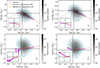 |
Fig. 2. Comparisons between the predictions from two geometry models and the observed fHα/fHβ–fX/fHα line ratios for Hγ, Hδ, P8, and P10. The magenta curves and shaded regions indicate the medians and their 3σ uncertainties of the binned distributions, respectively. In each panel, the red dashed line denotes the predicted relation based on the foreground screen dust model, while the orange dotted line is the prediction based on the uniform mixture model. The Fitzpatrick (1999) dust extinction curve with RV = 3.1 is assumed in both cases. The background gray map shows the logarithmic number density of our sample, while the cyan contours enclose 68%, 95%, and 99% of the H II region spaxels, respectively. The horizontal and vertical black lines indicate the intrinsic values of the corresponding ratios based on the Case B recombination. The median uncertainties of the sample are given in the lower-right corner. A close-up of the region around the cross point of the intrinsic line ratios is shown in the lower-left inset of each panel. |
3.2. Comparisons between the model-predicted and observed line ratios
We present the fHα/fHβ–fX/fHα line ratio diagrams (X = Hγ, Hδ, P8, and P10) in Fig. 2. In each panel, the background grayscale map is the spaxel number density on a logarithmic scale, while the magenta curve denotes the binned medians. The shaded regions around the median curves are their 3σ uncertainties, which is the central 99% percentile range of the distributions of the medians resampled via the bootstrapping method. For comparison, the predicted relations between these line ratios based on the foreground screen dust model (red dashed line) and uniform mixture model (orange dotted line) are also given by assuming the Fitzpatrick (1999) dust extinction curve with RV = 3.1 and the Case B recombination with electron temperature Te = 104 K and electron density ne = 100 cm−3. The intrinsic line ratios are computed via the PyNeb package (Luridiana et al. 2015) with the default recombination line data from Storey & Hummer (1995). Note that although Fig. 2 plots line ratios on a logarithmic scale, the median curves are computed on a linear scale. This consideration aims to avoid any bias arising from computing logarithmic line ratios for emission lines with zero fluxes since we do not apply any S/N cut on the targeted lines.
The inclusion of spaxels with low-S/N detections of emission lines leads to very large scatters in the distributions of our sample for all lines, especially for the Paschen lines. However, as expected, all the median curves generally follow a linear relation at fHα/fHβ ≳ 2.86 (i.e., the intrinsic Hα-to-Hβ ratio expected by the Case B recombination), which are consistent with the predictions based on the foreground screen model. Both the median curves and the number density contours extend to the unphysical region with fHα/fHβ ≲ 2.86, which is possible if the uncertainties are taken into account. Predictions of both dust models are generated with an E(B − V) range of 0 − 10 mag, which is large enough to account for the vast majority of H II regions even for starburst galaxies (Calabrò et al. 2018). Obviously, the major and crucial difference between the predictions of the two dust geometry models is that the foreground screen one has a much larger range in line ratios compared to the mixed mode. Due to the aforementioned line-ratio saturation effect, the uniform mixture model cannot predict a line ratio that is large enough to cover most of the observed line ratio ranges presented in Fig. 2 when the measurement uncertainties are not considered.
Large scatters and unphysical line ratios are also reported by Prescott et al. (2022), in which ground-based slit and space-based slitless grism spectra were combined to draw the line ratio diagram including Hα, Hβ, and Pβ. With their small sample, the authors attributed the scatters to the differences in the spatial covering factors between the Balmer and Paschen lines and/or the slit loss in ground-based observations. Our sample is large enough to demonstrate that even though observations were performed with the same instrument and reduced in the same manner, large scatters are still observable even for the line ratio plots including the Balmer lines only (i.e., the top panels of Fig. 2). In Section 3.3 we will show that the large coverages in the line ratio diagrams can be recovered via a simple simulation, in which the uncertainties in the emission-line measurements are taken into account without the need to differentiate the coverage factors of the Balmer or Paschen lines.
Furthermore, although the median curves between the logarithmic line ratios are in good agreement with a linear relation, the slopes seem to deviate slightly from the assumed Fitzpatrick (1999) values. We will return to this problem in Section 4. In Fig. 2, we also indicate the intrinsic fHα/fHβ and fX/fHα ratios predicted by the Case B recombination with the vertical and horizontal black solid lines, respectively. As revealed in Equation (7), one should expect that the median curves would go through the intersection points of two black lines if the Case B recombination is valid for our sample. However, deviations from the theoretical values are observed in all cases shown in Fig. 2. This inconsistency is exhibited more clearly in the zoom-in plots in the insets. We will elucidate this offset in Section 3.3 and attribute it to the measurement uncertainties of the emission-line fluxes and/or the night-sky line residuals rather than intrinsic deviation from the Case B recombination.
3.3. Simple simulation for two geometry models
Due to the large measurement uncertainties of line ratios, especially for the Paschen lines, the distributions of spaxels in the line ratio plots exhibit pretty large scatters around the median curve. Here we further provide a simple simulation to argue that the observed line ratio relations for most of our spaxels are better described by the foreground screen model rather than the uniform mixture model and confirm that the observed large scatters can be predominately explained by the large measurement uncertainties of emission lines.
During the simulation, we assumed the Fitzpatrick (1999) extinction curve with RV = 3.1 and the Case B recombination with Te = 104 K and ne = 100 cm−3. The procedure is as follows.
-
For all spaxels in our sample, the nebular color excesses E(B − V) and intrinsic (dust-corrected) Hα fluxes (fHα, int) for individual spaxels are computed from the observed Hα/Hβ ratio by assuming the geometry model that we want to simulate.
-
Due to the strong correlation between fHα, int and E(B − V) (i.e., the strong correlation between SFR and the nebular dust attenuation; Li et al. 2019), the derived intrinsic Hα fluxes are randomly matched with an E(B − V) value in a manner that forces the resulting fHα, int, sim–E(B − V)sim distribution to be similar to the observed one.
-
The simulated intrinsic fluxes of Hβ and other recombination lines X can be computed from fHα, int, sim under the Case B recombination assumption.
-
Based on the targeted dust geometry model and E(B − V)sim, the simulated true fluxes after dust attenuation for each recombination line (frec, sim, att) can be computed.
-
By assuming that the true attenuated flux, frec, sim, att, and their simulated uncertainties, σrec, sim, follow the observed frec, obs–σrec, obs distributions of our sample, we can randomly assign a σrec, sim to each frec, sim, att.
-
Finally, the simulated observed flux (frec, sim, obs) is obtained by assuming that the measurement uncertainty follows a Gaussian distribution with a mean of frec, sim, att and a standard deviation of σrec, sim.
In short, this simulation aims to reproduce the observed E(B − V)–fHα, int and frec, obs–σrec, obs relations. Although what we simulated is the frec, sim, att–σrec, sim relation in practice, we also compared the obtained frec, sim, obs–σrec, sim relation with the observed frec, obs–σrec, obs and find good agreements between them for all lines. To match our selection criteria described in Section 2.2, simulated spaxels with fHα, sim, obs/σHα, sim < 3 or fHβ, sim, obs/σHβ, sim < 3 were excluded from our simulated sample. Negative simulated fluxes due to the resampling from the Gaussian distribution might be obtained for some spaxels and were set to zero in the simulated catalogs. This setting is designed to mock the results of DAP, which forces the Gaussian flux to be non-negative. Thus, for non-detection, the fluxes could be zero. Given the line-ratio saturation in the uniform mixture model, about 12.6% of our sample cannot obtain valid attenuation estimations due to their too large Hα-to-Hβ ratios. Fig. 3 shows similar plots as Fig. 2 but adds the results for the simulated sample generated by assuming two considered geometry models. Since the Fitzpatrick (1999) extinction curve with RV = 3.1 was adopted in the simulation, the red dashed and orange dotted lines should be the true values of the median curves for the foreground screen model and uniform mixture model, respectively.
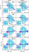 |
Fig. 3. Comparisons of the line ratio plots between the observations and the simulated samples generated by assuming the foreground screen dust model (left) and the uniform mixture model (right). In each panel, the filled contours and black contour lines indicate the spaxel distributions of the observed and simulated samples, respectively, both of which enclose 68%, 95%, and 99% of the corresponding samples from inner to outer. The magenta (blue) curve and shaded regions denote the medians and their 3σ uncertainties for the observed (simulated) sample, respectively. Regions around the cross points of the intrinsic line ratios are zoomed in and shown in the lower-left insets. The SSIM index describing the similarity in density distribution between the observed and simulated data is listed in the lower-right corner of each panel. Other symbols are the same as those in Fig. 2. |
We first compare the simulated median curves with their true values. For the foreground screen model, the simulated median curves are in good agreement with the true values, except for the regimes below the intrinsic Hα-to-Hβ ratio and the high-fHα/fHβ ends. Given that the Case B recombination was assumed in the simulation, the true values of the simulated attenuated Hα-to-Hβ ratios (fHα, sim, att/fHβ, sim, att) cannot be smaller than the intrinsic one, as shown by the red lines in Fig. 3. However, the introduced uncertainties when mocking observations make it possible for the “observed” values (fHα, sim, obs/fHβ, sim, obs) to go below the intrinsic one. In addition, when fHα/fHβ is at the intrinsic Case B value, the median simulated fX/fHα values would go below the intrinsic values, in exactly the same way as the observed trend for Hγ and Hδ. This is also due to the uncertainties introduced. Because uncertainties scatter spaxels around in both the horizontal direction and vertical direction in these plots, many spaxels with an observed Case B fHα/fHβ actually have nonzero intrinsic attenuation. Thus, their median fX/fHα should also display some level of attenuation. This also should be the reason for the small differences between the simulated median curves and their true values (i.e., the theoretical line) at the high-fHα/fHβ ends, except that now we underestimate attenuation due to large contamination by points with intrinsically lower fHα/fHβ ratios.
As for the uniform mixture model, due to the line-ratio saturation effect, fHα, sim, att/fHβ, sim, att has an upper limit at ∼4.39. Similarly, the introduction of uncertainties around the true values results in deviations from the orange dotted line. However, due to the narrow range of the true values in this model, the simulated median curves seem to deviate from the model predictions more or less in the whole range of fHα, sim, att/fHβ, sim, att, especially for the Hγ and Hδ lines. The uncertainties also can scatter a certain amount of spaxels to the high-fHα, sim, obs/fHβ, sim, obs end, beyond the theoretical upper limit of this line ratio.
Comparing with the observations exhibited in Fig. 2 (overplotted as filled contours and magenta curves in Fig. 3), we find that the simulation results from the foreground screen model are generally more consistent with our sample in terms of both the median curves and the overall distributions of spaxels. Given that the physical scale sampled by the MaNGA data is about 1–2 kpc, this result is in good agreement with Liu et al. (2013) in which the authors report that the foreground screen model becomes consistent with observations averaged over a scale of ≳100 − 200 pc. The apparent “non-Case B recombination” intercepts at the intrinsic Hα-to-Hβ ratios of Hγ and Hδ can be well reproduced by the simulation, indicating that these offsets can be attributed to the measurement uncertainties of emission lines only. For P8 and P10, the discrepancy between the simulated intercepts and the observed ones implies that additional factors other than the emission-line uncertainties should have nonnegligible effects on these weak line measurements, such as sky-night line residuals and/or zero fluxes from the Gaussian fitting (see Section 4.5).
As a sanity check, we adopted a structural similarity (SSIM) index proposed by Wang et al. (2004) to assess the similarity between the observed and simulated distributions for the two geometry models. The normalized 2D density distributions in logarithmic line ratio space (e.g., Fig. 2 after normalization) are used to create density images for the calculation. The density images are then pixelated to allow a pixel-by-pixel calculation of the SSIM index, which is implemented by the Python function skimage.metrics.structural_similarity. To describe the overall similarity between the two density images, we used the value weighted by the normalized number density of the observed data. Generally speaking, the overall SSIM index is between 0 and 1 with a larger value indicating more similarity in overall structure between two density images. The resulting SSIM indices of each line for both geometry models are given in the lower-right corner of the corresponding panels in Fig. 3.
For Hγ and Hδ, both geometry models give large SSIM indices (i.e., SSIM > 0.8) due to the following reasons: (1) the main difference between the two geometry models are at large Hα/Hβ values where the spaxel density already becomes smaller, and (2) the overall SSIM index is weighted by the normalized density distribution of the spaxels. The P8 and P10 lines have much smaller SSIM indices compared to Hγ and Hδ even for the foreground screen model, which implies that the assumptions and/or models involved in the current simulation are not enough to mock the emission-line measurements of the P8 and P10 lines. In other words, we are still far from understanding the flux measurements of these weak recombination lines. A similar conclusion is also implied by the fitting results shown in Section 4.4 and is further discussed in Section 4.5. For all lines shown in Fig. 3, the SSIM indices for the foreground screen model are all larger than the ones for the uniform mixture model, suggesting that the density distributions of the simulated catalogs based on the foreground screen model are more similar to the observed ones.
Overall, we conclude that for most of the spaxels in our sample, observations from all four recombination lines considered in this work favor the foreground screen dust model rather than the uniform mixture model. In the following analysis, we adopted this dust geometry as our fiducial one. The preferred dust geometry of ionized gas might depend on other physical properties. This topic is beyond the scope of this paper but is worthy of further investigation in a future paper.
4. Deriving the slope of the nebular attenuation
In this section, we derive the slope of nebular dust attenuation among hydrogen recombination lines (i.e., the slope in Equation (7)). This would lead to the constraints on the attenuation curve at those specific wavelengths.
4.1. Preliminary thinking and attempts toward the fitting method
Given Equation (7) and Fig. 2, the simplest and most straightforward way to constrain the slope of nebular dust attenuation is to fit the median curves displayed in Fig. 2 to a linear function directly (e.g., Prescott et al. 2022; Ji et al. 2023). However, this method has several problems. First, as demonstrated in Section 3.3, the measurement uncertainties have significant influences on the derived median curves, especially when the fHα, obs/fHβ, obs ratios are very close to the intrinsic value. Fig. 3 also suggests that, even for the foreground screen model, the simulated median curves could have small but detectable deviations from the true values at the large Balmer decrement end. These effects prevent us from determining a reasonable Hα-to-Hβ ratio range to perform the fitting. Second, when fitting median curves, although the uncertainties of the median values can be computed and taken into account in the fitting, the uncertainties of individual spaxels are difficult to handle and might be ignored in the fitting.
To fully consider the measurement uncertainties of individual spaxels, another method is to fit the logarithmic line ratios of all spaxels to a linear function. Although this method works for the Hγ and Hδ lines, it fails to provide reliable results for P8 and P10 since the best-fit slopes always have opposite signs to what we expected, and thus cannot match the observed median curves. One of the reasons for this strange issue is that, due to the faintness of the Paschen lines, the Gaussian fitting in the DAP resulted in zero flux for a large number of spaxels. Although the uncertainties are not zero for these spaxels, computing any logarithmic line ratios would remove them from our sample and inevitably bias the sample toward H II regions that have brighter and positively biased Paschen lines or are significantly contaminated by night-sky line residuals.
Furthermore, we note that it is difficult to properly take into account the uncertainties for logarithmic line ratios. The general error propagation formula provides a computable method to give symmetric uncertainty that is easy to take into account in the fitting. However, this symmetric uncertainty of the logarithmic line ratio is approximately correct only when the uncertainties are very small. On the other hand, during the fitting, we always assume that the uncertainties of observables (i.e., the logarithmic line ratios in this case) follow a Gaussian distribution, which is also the requirement for the conventional definition of likelihood function or χ2 merit function. But it might be not true for the logarithmic line ratios since the uncertainties of individual emission-line fluxes are naturally assumed to be Gaussian, and thus the logarithmic line ratios should not follow a Gaussian distribution anymore. Given these reasons, we propose a new fitting approach to fit the measured emission-line fluxes directly in this work.
4.2. A novel fitting method using emission line fluxes directly
In this section, we provide a brief introduction to our fitting method. This method aims to constrain the slope of the nebular attenuation curve using the measured emission-line fluxes directly so that the uncertainties involved in the likelihood function (or the χ2 definition) could be simply described by Gaussian distributions.
From Equation (7), we can define a relative slope between Hα, Hβ, and any other hydrogen recombination line (denoted as “X” hereafter) as
 (9)
(9)
Taking the Fitzpatrick (1999) Milky Way extinction curve with RV = 3.1 as the fiducial one, the observed slope for line X can be described as
 (10)
(10)
in which mX, F99 is the slope computed from the Milky Way curve and ΔmX is the difference in slope between the observed and fiducial values. For a fixed ΔmX, the nebular attenuation at the wavelength of line X can be computed
 (11)
(11)
During the fitting, we assumed that all spaxels in our sample follow the same nebular attenuation curve and treated ΔmX as a free parameter.
For each spaxel, we defined a likelihood function related to line X as
 (12)
(12)
where fi,pre is the predicted fluxes based on the considered dust attenuation curve and σi,obs is the uncertainty of emission-line flux. For a given attenuation curve and assuming the Case B recombination, we can compute all three predicted fluxes from the observed fluxes (fHα, obs, fHβ, obs, and fX, obs) with the knowledge of the intrinsic Hα flux (fHα, int) and the dust attenuation at the wavelength of Hα (AHα).6 In other words, for each spaxel, we took fHα, int and AHα as free parameters to obtain fi,pre. The posterior probability was computed from
 (13)
(13)
in which 𝒫prior is the prior probability and limits the valid range of the two parameters. Thus 𝒫prior can be written as
 (14)
(14)
For a given ΔmX, ln𝒫spaxel was maximized respectively for each spaxel by finding the best combination of fHα, int and AHα. We summed up the best-fit ln𝒫spaxel of individual spaxels to get the posterior probability of the whole sample for that ΔmX, namely
 (15)
(15)
Then we searched the best ΔmX that maximizes ln𝒫sample.
Additionally, we manually introduced a constant scaling factor c to the predicted flux fX, pre for each targeted recombination line, namely, the predicted flux is rewritten as
 (16)
(16)
This constant is invariant for all spaxels and could account for any systematic effects such as deviations from the Case B recombination and measurement systematics arising from the stellar continuum subtraction or night-sky line residuals. Moreover, a multiplicative systematic error in flux calibration would result in a different c but would not change ΔmX. We will show in Sections 4.4 and 4.5 that this constant is necessary for the fitting, especially for weak lines like P10. To avoid predicting negative fluxes, we used lgc as a free parameter in practice.
In short, the fitting procedure can be summarized as follows. We set ΔmX and c as free parameters for the whole sample. Given one (ΔmX, c) pair, fi,pre and thus lnℒspaxel can be derived by treating fHα, int and AHα as free parameters for individual spaxels. Maximizing ln𝒫spaxel for each spaxel will obtain the posterior probability of the (ΔmX, c) pair, which is then summed up to give ln𝒫sample. Finally, we maximized ln𝒫sample to obtain the best-fit (ΔmX, c) pair for the whole sample. The minimize function from the SciPy module was utilized to maximize ln𝒫spaxel for each spaxel. When maximizing ln𝒫sample, we first used the minimize function to minimize −ln𝒫sample and obtained an initial guess of the best-fit parameters, which was then fed to the emcee module (Foreman-Mackey et al. 2013) to perform a Markov chain Monte Carlo (MCMC; e.g., Sharma 2017) sampling after adding small random perturbations. The medians and 16th-84th percentile ranges of the posterior probability distributions constructed from the MCMC chains after discarding a certain fraction of initial steps (i.e., the so-called “burn-in” phase) were taken as the final best-fit parameters and their uncertainties, respectively.
It is noteworthy that although we adopted a specific curve (i.e., the Fitzpatrick 1999 curve with RV = 3.1) as a zero point for the parameter, ΔmX, during the fitting (see Equation (10)), the best-fit slopes (mX) are not dependent on that choice. More specifically, although the definition of the relative slope mX (Equation 9) involves the attenuation difference between Hα and Hβ, which is computed by assuming a certain attenuation curve, replacing this curve with other attenuation curves (e.g., the Calzetti et al. 2000 curve) in the fitting would change the best-fit ΔmX but keep the best-fit mX unchanged. The proof is given in Appendix C.
Our method has the following advantages. First, using the emission-line fluxes directly in the fitting instead of the logarithmic line ratios naturally avoids bias from the propagated uncertainties of line ratios which are asymmetric and non-Gaussian. Second, although the Case B recombination was assumed in the fitting, any deviations from it can be accounted for by the constant c and thus do not influence the determination of ΔmX. Other systematic uncertainties due to data reduction also can be handled in the same manner, as long as they are multiplicative in nature. Third, the inconsistency between the simulated median curves and their true values due to measurement uncertainties described in Section 3.3 can be naturally taken into account without the need to set a fitting range subjectively (see Section 4.4).
4.3. Simulation validation for the fitting procedure
4.3.1. Overall performance at different S/N thresholds
To evaluate the recovery ability and possible systematic uncertainty of the fitting method, we generated simulated samples with different S/N thresholds for Hα and Hβ, ranging from 3 to 100. The simulation procedure is the same as the one described in Section 3.3, but only the foreground screen dust model was applied. To mock different extents of deviations from the Milky Way extinction curve, we adopted a series of true ΔmX ranging from −0.3 to 0.3 with a step of 0.1 for all targeted line X. No deviation from the Case B recombination was assumed, meaning that the true value ctrue = 1. The simulated catalogs were then fed to the fitting process to obtain the best-fit parameter pair (ΔmX, c) for each case. Because implementing the full minimize-MCMC fitting procedure described in Section 4.2 is very expensive computationally, we only used the minimize step to derive the best-fit results of the simulated catalogs to save the computing time.
Fig. 4 exhibits how the differences between the recovered and true values of the parameters (ΔmX and c) vary as a function of the S/N cut applied to Hα and Hβ. Note that for the targeted line X (i.e., Hγ, Hδ, P8, and P10), we did not apply any S/N cut. It is not a surprise to see that the deviations from the true values of the two parameters become significantly larger for simulated samples with lower S/N cut on Hα and Hβ, regardless of the targeted lines. It seems that the fitting process provides an almost unbiased estimation of (ΔmX, c) only for the simulated samples with S/Ncut ≳ 50. Further inspection reveals that such deviations show very strong correlations with the fractions of spaxels that are set to zero fluxes in the simulated catalogs (see Section 3.3). As the adopted S/N threshold decreases, more spaxels with weak recombination lines are included in the sample. As a result, the fractions of spaxels that have zero fluxes in the corresponding simulated catalogs increase and thus bias the distribution of the targeted line X, leading to a biased best-fit result. Since the zero-flux setting in the simulation aims to mock the results of the non-negative Gaussian fitting implemented in the DAP, similar situations should also exist in the observational data. Fig. 4 also implies that the deviations of both free parameters are dependent on the true ΔmX values, especially when the deviations are not too large (i.e., Hγ and Hδ), suggesting that applying a simple correction to the best-fit values to obtain an unbiased estimation seems to be infeasible. The coincident trends of the differences in ΔmX and c reflect that the two parameters are degenerate to some extent, which can be confirmed via the posterior distributions (see Section 4.4).
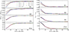 |
Fig. 4. Differences between the recovered and true values of the free parameters Δm (left) and c (right) as a function of the adopted Hα and Hβ S/N thresholds ranging from 3 to 100. Results based on the simulated catalogs with different true Δm are delineated by different colors. The fitting procedure to derive the best-fit parameters only includes the minimize step for saving computing resources. |
4.3.2. Fitting subsample selected by SFR surface density
As demonstrated in the last subsection, determining the nebular dust attenuation curve using the whole sample (i.e., star-forming spaxel sample with S/N threshold of 3 for Hα and Hβ) would inevitably introduce substantial systematic bias that is difficult to correct. We thus consider constructing a more conservative subsample to perform the fitting. Simply adopting an S/N cut at 50 will leave only 9.5% of the original sample, for which the sample size is too small and might not be representative of star-forming regions in the low-redshift Universe. On the other hand, since S/Ns of emission lines strongly depend on the exposure time and observation conditions, we instead performed the subsample selection using another physical parameter, the deprojected SFR surface density (ΣSFR, cor). When computing ΣSFR, cor, the Fitzpatrick (1999) Milky Way extinction curve with RV = 3.1 was adopted to correct dust attenuation of Hα fluxes. SFR was calculated from the dust-corrected Hα luminosity adopting the Kennicutt (1998) conversion relation under the Salpeter (1955) initial mass function assumption. We also retrieved the axis ratio from the NASA-Sloan Atlas catalog (Blanton et al. 2011; Albareti et al. 2017), which is derived from a single-component Sérsic fit in r-band, to correct for the projection effect due to the inclination (e.g., Barrera-Ballesteros et al. 2016).
Although the S/N selection mentioned in Fig. 4 was applied to both the Hα and Hβ lines, it should be dominated by the Hβ threshold due to the weaker nature of Hβ. We thus present the distribution of the main sample (S/Ncut = 3) on the S/N(Hβ)–ΣSFR, cor plane in Fig. 5 to illustrate our ΣSFR, cor-based sample selection. Our fitting subsample only includes ∼6.9 × 10⁵ spaxels with −2 ≤ logΣSFR, cor[M⊙ yr−1 kpc−2]< − 1, which account for nearly 20% of the main sample. Fewer than 1% of the spaxels at the highest ΣSFR, cor end are excluded due to the consideration of removing extreme regions. The lower limit of our ΣSFR, cor criterion is very close to the suggested boundary between H II-dominated and DIG-dominated spaxels for the MaNGA survey (blue dashed line in Fig. 5) proposed by Zhang et al. (2017), making sure that spaxels in this subsample are mainly excited by young massive OB stars. Although only 38.7% of spaxels in this ΣSFR, cor-selected sample have S/N(Hβ) > 50, we will demonstrate in the following that a nearly unbiased estimation of ΔmX can be derived from this subsample.
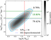 |
Fig. 5. S/N of Hβ as a function of the corrected SFR surface density. The vertical red dashed line indicates S/NHβ = 50, while the blue dashed line is the selection criterion of H II region-dominated spaxels for the MaNGA survey proposed by Zhang et al. (2017). The two green horizontal lines locate ΣSFR, cor = 0.01 and 0.1 M⊙yr−1kpc−2, respectively. The three percentages suggest the fractions of spaxels within each ΣSFR, cor bin. Spaxels between the green lines are adopted as the subsample to fit the slopes of the nebular dust attenuation curve. The underlying gray map and cyan contours are the same as those in Fig. 1. |
Based on the new fitting subsample, we generated 10 simulated catalogs following the procedure described in Section 3.3 but with different random seeds. Again, the true ΔmX varies from −0.3 to 0.3 with a step of 0.1 and ctrue = 1. The means and standard deviations of the differences between the true values and the best-fit ones derived from the minimization step for the ΣSFR, cor-selected sample are presented in Fig. 6.
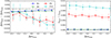 |
Fig. 6. Differences between the true and recovered Δm (using the minimize step only) as a function of the true Δm for our ΣSFR, cor-selected sample. The symbols with error bars indicate the means and standard deviations of the best-fit parameters for the 10 simulated samples in each case, respectively. |
Compared with the true ΔmX values, we still obtain best-fit results with deviations for the fitting sample. However, such deviations are greatly reduced by more than one order of magnitude compared to the simulated results for the S/Ncut = 3 samples presented in Fig. 4 and will be treated as corrections to our best-fit results derived from the minimization-MCMC procedure. Even for the Paschen lines, the deviations in the relative slopes are ≲0.008 in all cases, while the deviations in the scaling factor c are smaller than 1%.
From the posterior distributions provided by the MCMC, we can calculate the statistical uncertainties of the best-fit parameters, which is due to the emission-line measurement uncertainties and the size of the fitting sample. On the other hand, systematic uncertainties arising from imperfect data analysis, the adopted assumptions, and/or the fitting method cannot be assessed from the MCMC procedure and are difficult to account for. However, given the simulation described here, we can quantify these uncertainties to some extent. To this end, we computed the average deviations in ΔmX for each targeted line by averaging over all assumed true ΔmX. Note that the subtle trends of larger true ΔmX values having larger deviations for P8 and P10 are ignored due to the small variations over the simulated ΔmX range. The means and standard deviations of the deviations in ΔmX are −0.001 ± 0.001, −0.001 ± 0.001, −0.005 ± 0.003, and −0.005 ± 0.004 for Hγ, Hδ, P8, and P10, respectively. The standard deviations for Hγ and Hδ are smaller than 0.0005 but are rounded to 0.001 for conservative estimation of the uncertainties. Other hydrogen recombination lines (e.g., from H7 to H12 and P9) were also considered in the simulation and processed in the same manner, and the corresponding average deviations from the true values are given in Table 1.
Best-fit parameters from the minimization-MCMC procedure.
4.4. Minimization-MCMC results for the ΣSFR, cor-selected sample
We applied the minimization-MCMC fitting procedure to the ΣSFR, cor-selected sample to determine the best-fit relative slopes for star-forming regions on kpc scales. The best-fit results for the four main targeted lines are given in Fig. 7. For each targeted line, we provide a corner plot to display the posterior distributions of the parameters and an Hα/Hβ–X/Hα line ratio diagram to show the comparison between the observed median curve and the prediction based on the best-fit parameters. From the fitting, we took the medians and the 16th-84th percentile ranges of the posterior distributions as the best-fit parameters and 1σ uncertainties, respectively, for ΔmX and c.
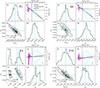 |
Fig. 7. Best-fit results for the four main recombination lines derived from the minimization-MCMC fitting method. In each case, Panel (c) shows the posterior probability distribution of the two parameters, while Panels (a) and (d) are the marginalized distributions of individual parameters. The cyan solid lines in these panels locate the medians of the corresponding distributions, and the cyan dashed lines enclose the 16th-84th percentile ranges of the distributions. The fit-best results with 1σ uncertainties (i.e., the 16th-84th percentile ranges) for ΔmX and c are listed in Panel (c). Panel (b) gives the comparison between the best-fit relation (green line) and the observed median curve (magenta curve) on the line ratio plane. Other symbols are similar to those in Fig. 2 but for the ΣSFR, cor-selected sample. |
For Hγ and Hδ, the scaling factors are ≲1%, which are much smaller than the median measurement uncertainties of these two lines in the fitting subsample. These negligible deviations for predicted fluxes demonstrate the reliability of the Case B recombination assumption for most of the spaxels in our sample and the accuracy of MaNGA’s relative flux calibration among these lines7. Hence, the relative slopes for these two lines can be well constrained. However, the best-fit c values for P8 and P10 suggest that the predicted fluxes from the Case B recombination should be reduced by about 9% and 31%, respectively, to match the observations. Thus, we have more complex situations for these two lines. We will discuss possible reasons for these systematic biases in Section 4.5. Intriguingly, the posterior distribution of the two parameters for P8 has a double-peak feature, leading to bimodal probability distributions for individual parameters. Although we have no idea about the reason for this odd feature that is different from other emission lines (also see Fig. B.2), the overall parameter space is still narrow and results in 1σ uncertainties of < 0.001 for both parameters.
The best-fit ΔmX are very small for Hγ and Hδ, while larger deviations are obtained for two Paschen lines. Although we did not fit the median curves directly, the best-fit relations between the line ratios are generally consistent with the median ones at fHα/fHβ ≳ 2.86 except for the P10 line. If the best-fit relations for Hγ, Hδ, and P8 are treated as the “true” values of the fitting sample, the offsets of the observed median curves from these “true” values are qualitatively in line with the ones between the simulated median curves and the foreground screen model predictions (i.e., also the true values in the simulation) shown in Fig. 3. This suggests that the scattering in line ratios due to the measurement uncertainties of emission-line fluxes discussed in Section 3.3 is naturally taken into account by our fitting approach. As a result, an unbiased estimate of the slope can be obtained. This is one of our motivations for developing a new fitting method.
As mentioned above, the uncertainties obtained from this procedure are only the statistical ones accounting for the uncertainties from emission-line measurements. As shown in Fig. 7, the derived uncertainties from this source for both free parameters are very small, regardless of the targeted lines, due to the large number of spaxels in our fitting sample. Together with the corrections and systematic uncertainties derived from Section 4.3.2, we can obtain the final estimations for ΔmX and c and list them in Table 1. The best-fit parameters from the minimization-MCMC procedure only, the differences between the best-fit and true values based on the simulation (i.e., systematic uncertainties), and the final estimation of the relative slope (mfinal) for each recombination line are also given. We emphasize that, theoretically, the derived mfinal is independent of the reference extinction or attenuation curve adopted in the fitting (see Appendix C) and thus can be directly compared with the predictions of different curves. For simplicity, the asymmetric uncertainties drawn from the posterior distributions in the MCMC fitting step are adjusted to be symmetric by adopting the larger side, although the exact asymmetric uncertainties are still listed in Fig. 7.
We find that the deviation of mHγ from the Fitzpatrick (1999) value is small but significant given the very small uncertainty. When applying to a region with E(B − V) = 0.6 mag8, this could result in a difference of about 3.6% in the dust correction factor compared to the standard Fitzpatrick (1999) extinction curve with RV = 3.1. The final best-fit ΔmHδ (ΔmH7) only contributes to an additional 1.0% (1.2%) of the dust correction in the same region. Such small corrections (together with the result for H7, see Section B) imply that the nebular dust attenuation on kpc scales can be described by the Fitzpatrick (1999) extinction curve within an accuracy of about 4% in terms of the dust correction factor. However, when comparing with the Calzetti et al. (2000) attenuation curve with RV = 4.05, similar corrections in the dust corrected fluxes are 5.1%, 5.6%, and 8.1% for Hγ, Hδ, and H7, respectively. For the Paschen lines, due to the degeneracy between ΔmX and c and the large departures of c from 1, their slopes could not be considered as well constrained before the sources of the non-unity c are resolved and quantified. Therefore, we conclude that only mX of strong recombination lines like Hγ, Hδ, and H7 can be well constrained given the current emission-line measurements.
4.5. Possible reasons for the non-unity scaling factors
Both Fig. 7 and Table 1 show that a scaling factor c smaller than 1 is required for P8 and P10 to let the predicted fluxes match with the observations. Possible reasons that might contribute to these systematic reductions are deviations from the Case B recombination assumption, improper stellar continuum subtraction, residuals of night-sky lines, improper emission-line measurements, and so on. Given the excellent agreements with Case B for Hγ, Hδ, and H7 (see Table 1), it is unlikely that this large offset from 1 is due to the intrinsic deviations from Case B predictions.
Because the sky residuals at the red end (around the Paschen lines) are still observable in some spectra, we have tried to remove this contamination by constructing an average template of night-sky line residuals for each Paschen line using emission-line fluxes from the DAP catalog. The resulting templates exhibit abundant night-sky lines, most of which are much stronger than the flux levels of the Paschen lines extracted from the DAP catalog. Although the fitting using the line fluxes after correcting for these sky residuals can have slightly smaller reduced χ2, the large uncertainties of such corrections are difficult to estimate. We thus did not apply these corrections in the fitting results presented in this work and left this issue for future study in which we will construct the templates from the MaNGA spectra directly (e.g., Yan 2011).
Another important effect of the Paschen lines is the zero-flux problem. Since we did not apply an S/N cut for our targeted lines, all spaxels with unmasked Gaussian fitting fluxes were included in the sample. For very weak emission lines, DAP might return zero fluxes with nonzero uncertainties. As a result, even for the ΣSFR, cor-selected subsample, the fractions of spaxels with zero fluxes are about 18% and 15% for P8 and P10, respectively 9. If the emission-line fluxes are measured by the means of fitting by a non-negative single Gaussian profile, the zero-flux problem is inevitable and significant given the faintness of the Paschen lines. The problem would depress the observed fluxes systematically and thus lead to a scaling factor smaller than 1, which aligns with our fitting results shown in Fig. 7. However, the dominant effect is difficult to determine and resolve with the current data.
The best-fit results listed in Table 1 for other recombination lines also demonstrate that the non-unity scaling factor problem also exists for the high-order Balmer lines (except H7) and P9. The P9 line has a very similar situation to those of P8 and P10. For the high-order Balmer series, we defer the discussion to Appendix B and briefly summarize here that either the imperfect stellar continuum modeling or the zero-flux problem of weak lines might play an important role in the scaling factor c.
5. Summary
In this work, we use the complete data release of the MaNGA survey to investigate the nebular dust attenuation curve for star-forming regions on kpc scales. We examine the dust geometry models observed by the hydrogen recombination lines via simple simulations. We propose a novel approach to fit the relative slopes of the nebular dust attenuation curve with emission-line fluxes directly and apply it to a ΣSFR, cor-selected subsample. Our main results are as follows.
-
Most of the star-forming regions favor the foreground screen dust model on kpc scales rather than the uniform mixture model.
-
Based on an ideal simulation considering Gaussian statistical flux uncertainties only, we find that our minimization-MCMC fitting procedure can recover the true values for both the slopes of the nebular dust attenuation curve and the scaling factors with nearly no bias for Hγ, Hδ, P8, and P10 for either high-S/N sample or the corresponding ΣSFR, cor-selected sample.
-
By applying the method to the MaNGA data (i.e., the ΣSFR, cor-selected subsample), we find that the relative slope of the nebular attenuation curve can be well determined for strong hydrogen recombination lines (e.g., Hγ, Hδ, and H7). However, severe contaminations and/or systematic uncertainties prevent us from obtaining reasonable values of the slopes and intercepts for weak recombination lines (e.g., the high-order Balmer lines or the Paschen lines).
-
For the H II region-dominated spaxels, the relative slopes of the nebular attenuation curve at the wavelengths of Hγ, Hδ, and H7 can be well described by the Fitzpatrick (1999) Milky Way extinction curve with RV = 3.1 with an accuracy in the corrected flux of ≲4%.
-
Implied by both the simulation and fitting results, emission-line fluxes obtained from non-negative Gaussian fitting are biased in the weak-line regime.
Our results further reveal that although the emission-line measurements from the DAP are very accurate for strong lines, the measurements for weak lines still suffer many problems, e.g., significant residuals of the night-sky line at the red end of spectra and improper stellar continuum subtraction at the blue end. The Gaussian fitting might also be problematic for weak lines where the fitting process might fit a nearby noise or directly return zero fluxes. To mitigate this problem, we are currently using optimal extraction (e.g., Horne 1986) to produce unbiased flux measurements for emission lines in the MaNGA spectra and hope to have a better flux estimator for weak lines. Overall, more accurate emission-line measurements are needed to better constrain the shape of the nebular dust attenuation curve.
By definition, dust extinction describes light loss along individual sightlines, including dust absorption and scattering out of the sightline, which is typical for point sources like stars and quasars. For extended sources, the geometry between the emitters and dust should be considered, and thus additional effects (such as dust scattering into the sightline and varying dust column densities along different sightlines) should be taken into account, which is referred to as dust attenuation.
The MaNGA DAP corrects for the Milky Way foreground extinction before performing both the stellar continuum and emission-line fittings, meaning that all emission-line measurements in the catalogs have been corrected for the Milky Way foreground dust. The correction uses the E(B − V) values from the Schlegel et al. (1998) maps and adopts the Milky Way extinction curve of O’Donnell (1994).
For convenience, we use “Hn” (“Pn”) to denote one Balmer (Paschen) line arising from a transition with an upper atomic level of n when n ≥ 7 (8) (e.g., Berg et al. 2015). For example, Hϵ will be denoted as H7 hereafter.
One should note that the N2, S2, and R3 indexes used here are all insensitive to dust correction due to the very small wavelength differences between the lines involved in each index. Therefore, the choice of dust extinction or attenuation curve should not have a significant influence on the sample selection. We also plot the dust attenuation vector indicating E(B − V) = 1 mag in Fig. 1 for reference.
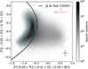 |
Fig. 1. Distribution of the S/N-selected spaxels in the P1–P2 diagram. The black solid curve is the H II region selection function given by Ji & Yan (2020). The background grayscale map shows the number density distribution of all the S/N-selected spaxels, while the cyan contours enclose 68%, 95%, and 99% of the H II region spaxels only, respectively. The median uncertainties of the S/N-selected sample are given in the lower-right corner, while the dust attenuation vector indicating E(B − V) = 1 mag is shown in the upper-right corner. |
Here we do not introduce any variation in kHβ − kHα, thus AHβ can be computed from AHα with the fiducial extinction curve.
It might be possible that both cases are not true and bias the predicted fluxes by a similar amount but with different signs, and thus a ∼1 scaling factor is still returned by the fitting procedure. However, it is nearly impossible that this coincidence happens simultaneously for three emission lines (i.e., Hγ, Hδ, and H7, see Table 1 and Fig. B.2)
Note that the E(B − V) of 99% spaxels in the S/Ncut = 3 sample are < 0.6 mag when a Fitzpatrick (1999) extinction curve is assumed.
The P10 line should have a smaller intrinsic flux but suffer more dust attenuation compared to the P8 line. Contrary to what is observed, we thus should expect more spaxels with zero fluxes for P10 rather than P8. This conflict might reflect the contamination of the sky residuals.
Here we can treat this fixed slope as the best-fit one.
Acknowledgments
We would like to thank the anonymous referee for the very helpful comments. Z.S.L. would like to thank Xihan Ji for his valuable discussion during the preparation of this work. We acknowledge the support by the Research Grant Council of Hong Kong (Project No. 14302522) and the National Natural Science Foundation of China (NSFC; grant No. 12373008). Z.S.L. acknowledges the support from Hong Kong Innovation and Technology Fund through the Research Talent Hub program (PiH/022/22GS). RY acknowledges support by the Hong Kong Global STEM Scholar Scheme (GSP028), by the Hong Kong Jockey Club Charities Trust through the project, JC STEM Lab of Astronomical Instrumentation and Jockey Club Spectroscopy Survey System, and by the NSFC Distinguished Young Scholars Fund (grant No. 1242500304). Funding for the Sloan Digital Sky Survey IV has been provided by the Alfred P. Sloan Foundation, the U.S. Department of Energy Office of Science, and the Participating Institutions. SDSS-IV acknowledges support and resources from the Center for High Performance Computing at the University of Utah. The SDSS website is http://www.sdss4.org. SDSS-IV is managed by the Astrophysical Research Consortium for the Participating Institutions of the SDSS Collaboration including the Brazilian Participation Group, the Carnegie Institution for Science, Carnegie Mellon University, Center for Astrophysics | Harvard & Smithsonian, the Chilean Participation Group, the French Participation Group, Instituto de Astrofísica de Canarias, The Johns Hopkins University, Kavli Institute for the Physics and Mathematics of the Universe (IPMU) / University of Tokyo, the Korean Participation Group, Lawrence Berkeley National Laboratory, Leibniz Institut für Astrophysik Potsdam (AIP), Max-Planck-Institut für Astronomie (MPIA Heidelberg), Max-Planck-Institut für Astrophysik (MPA Garching), Max-Planck-Institut für Extraterrestrische Physik (MPE), National Astronomical Observatories of China, New Mexico State University, New York University, University of Notre Dame, Observatário Nacional / MCTI, The Ohio State University, Pennsylvania State University, Shanghai Astronomical Observatory, United Kingdom Participation Group, Universidad Nacional Autónoma de México, University of Arizona, University of Colorado Boulder, University of Oxford, University of Portsmouth, University of Utah, University of Virginia, University of Washington, University of Wisconsin, Vanderbilt University, and Yale University.
References
- Abdurro’uf, Accetta, K., Aerts, C., et al. 2022, ApJS, 259, 35 [NASA ADS] [CrossRef] [Google Scholar]
- Albareti, F. D., Allende Prieto, C., Almeida, A., et al. 2017, ApJS, 233, 25 [Google Scholar]
- Baldwin, J. A., Phillips, M. M., & Terlevich, R. 1981, PASP, 93, 5 [Google Scholar]
- Barrera-Ballesteros, J. K., Heckman, T. M., Zhu, G. B., et al. 2016, MNRAS, 463, 2513 [NASA ADS] [CrossRef] [Google Scholar]
- Battisti, A. J., Calzetti, D., & Chary, R.-R. 2016, ApJ, 818, 13 [NASA ADS] [CrossRef] [Google Scholar]
- Battisti, A. J., Calzetti, D., & Chary, R.-R. 2017, ApJ, 840, 109 [NASA ADS] [CrossRef] [Google Scholar]
- Battisti, A. J., Bagley, M. B., Baronchelli, I., et al. 2022, MNRAS, 513, 4431 [NASA ADS] [CrossRef] [Google Scholar]
- Bautista, M. A., Pogge, R. W., & Depoy, D. L. 1995, ApJ, 452, 685 [NASA ADS] [CrossRef] [Google Scholar]
- Belfiore, F., Westfall, K. B., Schaefer, A., et al. 2019, AJ, 158, 160 [CrossRef] [Google Scholar]
- Berg, D. A., Skillman, E. D., Croxall, K. V., et al. 2015, ApJ, 806, 16 [NASA ADS] [CrossRef] [Google Scholar]
- Blanton, M. R., Kazin, E., Muna, D., Weaver, B. A., & Price-Whelan, A. 2011, AJ, 142, 31 [NASA ADS] [CrossRef] [Google Scholar]
- Blanton, M. R., Bershady, M. A., Abolfathi, B., et al. 2017, AJ, 154, 28 [Google Scholar]
- Bundy, K., Bershady, M. A., Law, D. R., et al. 2015, ApJ, 798, 7 [Google Scholar]
- Calabrò, A., Daddi, E., Cassata, P., et al. 2018, ApJ, 862, L22 [Google Scholar]
- Calabrò, A., Pentericci, L., Feltre, A., et al. 2023, A&A, 679, A80 [NASA ADS] [CrossRef] [EDP Sciences] [Google Scholar]
- Calzetti, D. 1997, Am. Inst. Phys. Conf. Ser., 408, 403 [NASA ADS] [Google Scholar]
- Calzetti, D. 2001, PASP, 113, 1449 [Google Scholar]
- Calzetti, D., Kinney, A. L., & Storchi-Bergmann, T. 1994, ApJ, 429, 582 [Google Scholar]
- Calzetti, D., Kinney, A. L., & Storchi-Bergmann, T. 1996, ApJ, 458, 132 [NASA ADS] [CrossRef] [Google Scholar]
- Calzetti, D., Armus, L., Bohlin, R. C., et al. 2000, ApJ, 533, 682 [NASA ADS] [CrossRef] [Google Scholar]
- Calzetti, D., Battisti, A. J., Shivaei, I., et al. 2021, ApJ, 913, 37 [CrossRef] [Google Scholar]
- Cappellari, M., & Copin, Y. 2003, MNRAS, 342, 345 [Google Scholar]
- Cardelli, J. A., Clayton, G. C., & Mathis, J. S. 1989, ApJ, 345, 245 [Google Scholar]
- Charlot, S., & Fall, S. M. 2000, ApJ, 539, 718 [Google Scholar]
- Chevallard, J., Charlot, S., Wandelt, B., & Wild, V. 2013, MNRAS, 432, 2061 [CrossRef] [Google Scholar]
- Cleri, N. J., Trump, J. R., Backhaus, B. E., et al. 2022, ApJ, 929, 3 [NASA ADS] [CrossRef] [Google Scholar]
- Dole, H., Lagache, G., Puget, J.-L., et al. 2006, A&A, 451, 417 [NASA ADS] [CrossRef] [EDP Sciences] [Google Scholar]
- Domínguez-Guzmán, G., Rodríguez, M., García-Rojas, J., Esteban, C., & Toribio San Cipriano, L. 2022, MNRAS, 517, 4497 [CrossRef] [Google Scholar]
- Draine, B. T. 2003, ARA&A, 41, 241 [NASA ADS] [CrossRef] [Google Scholar]
- Drory, N., MacDonald, N., Bershady, M. A., et al. 2015, AJ, 149, 77 [CrossRef] [Google Scholar]
- Fitzpatrick, E. L. 1999, PASP, 111, 63 [Google Scholar]
- Foreman-Mackey, D., Hogg, D. W., Lang, D., & Goodman, J. 2013, PASP, 125, 306 [Google Scholar]
- González Delgado, R. M., Leitherer, C., & Heckman, T. M. 1999, ApJS, 125, 489 [CrossRef] [Google Scholar]
- Gordon, K. D., Calzetti, D., & Witt, A. N. 1997, ApJ, 487, 625 [CrossRef] [Google Scholar]
- Greve, A. 2010, A&A, 518, A62 [NASA ADS] [CrossRef] [EDP Sciences] [Google Scholar]
- Greve, A., Castles, J., & McKeith, C. D. 1994, A&A, 284, 919 [NASA ADS] [Google Scholar]
- Groves, B., Brinchmann, J., & Walcher, C. J. 2012, MNRAS, 419, 1402 [NASA ADS] [CrossRef] [Google Scholar]
- Horne, K. 1986, PASP, 98, 609 [Google Scholar]
- Ji, X., & Yan, R. 2020, MNRAS, 499, 5749 [NASA ADS] [CrossRef] [Google Scholar]
- Ji, X., & Yan, R. 2022, A&A, 659, A112 [NASA ADS] [CrossRef] [EDP Sciences] [Google Scholar]
- Ji, X., Yan, R., Bundy, K., et al. 2023, A&A, 670, A125 [NASA ADS] [CrossRef] [EDP Sciences] [Google Scholar]
- Kauffmann, G., Heckman, T. M., Tremonti, C., et al. 2003, MNRAS, 346, 1055 [Google Scholar]
- Kennicutt, R. C., Jr 1998, ARA&A, 36, 189 [NASA ADS] [CrossRef] [Google Scholar]
- Kennicutt, R. C., & Evans, N. J. 2012, ARA&A, 50, 531 [NASA ADS] [CrossRef] [Google Scholar]
- Kewley, L. J., & Ellison, S. L. 2008, ApJ, 681, 1183 [Google Scholar]
- Kewley, L. J., Dopita, M. A., Sutherland, R. S., Heisler, C. A., & Trevena, J. 2001, ApJ, 556, 121 [Google Scholar]
- Kewley, L. J., Nicholls, D. C., & Sutherland, R. S. 2019, ARA&A, 57, 511 [Google Scholar]
- Kreckel, K., Groves, B., Schinnerer, E., et al. 2013, ApJ, 771, 62 [NASA ADS] [CrossRef] [Google Scholar]
- Law, D. R., Yan, R., Bershady, M. A., et al. 2015, AJ, 150, 19 [CrossRef] [Google Scholar]
- Law, D. R., Cherinka, B., Yan, R., et al. 2016, AJ, 152, 83 [Google Scholar]
- Li, H., Wuyts, S., Lei, H., et al. 2019, ApJ, 872, 63 [NASA ADS] [CrossRef] [Google Scholar]
- Li, N., Li, C., Mo, H., et al. 2020, ApJ, 896, 38 [NASA ADS] [CrossRef] [Google Scholar]
- Lin, Z., & Kong, X. 2020, ApJ, 888, 88 [NASA ADS] [CrossRef] [Google Scholar]
- Lin, Z., Hu, N., Kong, X., et al. 2017, ApJ, 842, 97 [NASA ADS] [CrossRef] [Google Scholar]
- Liu, G., Calzetti, D., Hong, S., et al. 2013, ApJ, 778, L41 [CrossRef] [Google Scholar]
- Luridiana, V., Morisset, C., & Shaw, R. A. 2015, A&A, 573, A42 [NASA ADS] [CrossRef] [EDP Sciences] [Google Scholar]
- Mesa-Delgado, A., Esteban, C., García-Rojas, J., et al. 2009, MNRAS, 395, 855 [NASA ADS] [CrossRef] [Google Scholar]
- Narayanan, D., Conroy, C., Davé, R., Johnson, B. D., & Popping, G. 2018, ApJ, 869, 70 [Google Scholar]
- Natta, A., & Panagia, N. 1984, ApJ, 287, 228 [NASA ADS] [CrossRef] [Google Scholar]
- O’Donnell, J. E. 1994, ApJ, 422, 158 [Google Scholar]
- Osterbrock, D. E. 1989, Astrophysics of Gaseous Nebulae and Active Galactic Nuclei (University Science Books) [Google Scholar]
- Paradis, D., Mény, C., Demyk, K., Noriega-Crespo, A., & Ristorcelli, I. 2023, A&A, 674, A141 [NASA ADS] [CrossRef] [EDP Sciences] [Google Scholar]
- Petersen, L., & Gammelgaard, P. 1996, A&A, 308, 49 [NASA ADS] [Google Scholar]
- Petersen, L., & Gammelgaard, P. 1997, A&A, 323, 697 [NASA ADS] [Google Scholar]
- Prescott, M. K. M., Finlator, K. M., Cleri, N. J., Trump, J. R., & Papovich, C. 2022, ApJ, 928, 71 [NASA ADS] [CrossRef] [Google Scholar]
- Price, S. H., Kriek, M., Brammer, G. B., et al. 2014, ApJ, 788, 86 [NASA ADS] [CrossRef] [Google Scholar]
- Qin, J., Zheng, X. Z., Wuyts, S., Pan, Z., & Ren, J. 2019, ApJ, 886, 28 [NASA ADS] [CrossRef] [Google Scholar]
- Reddy, N. A., Kriek, M., Shapley, A. E., et al. 2015, ApJ, 806, 259 [NASA ADS] [CrossRef] [Google Scholar]
- Reddy, N. A., Shapley, A. E., Kriek, M., et al. 2020, ApJ, 902, 123 [NASA ADS] [CrossRef] [Google Scholar]
- Reddy, N. A., Topping, M. W., Sanders, R. L., Shapley, A. E., & Brammer, G. 2023, ApJ, 948, 83 [NASA ADS] [CrossRef] [Google Scholar]
- Relaño, M., Kennicutt, R., Lisenfeld, U., et al. 2016, A&A, 595, A43 [NASA ADS] [CrossRef] [EDP Sciences] [Google Scholar]
- Relaño, M., De Looze, I., Kennicutt, R. C., et al. 2018, A&A, 613, A43 [NASA ADS] [CrossRef] [EDP Sciences] [Google Scholar]
- Rezaee, S., Reddy, N., Shivaei, I., et al. 2021, MNRAS, 506, 3588 [CrossRef] [Google Scholar]
- Salim, S., & Narayanan, D. 2020, ARA&A, 58, 529 [NASA ADS] [CrossRef] [Google Scholar]
- Salpeter, E. E. 1955, ApJ, 121, 161 [Google Scholar]
- Schlegel, D. J., Finkbeiner, D. P., & Davis, M. 1998, ApJ, 500, 525 [Google Scholar]
- Scoville, N., Faisst, A., Capak, P., et al. 2015, ApJ, 800, 108 [NASA ADS] [CrossRef] [Google Scholar]
- Seon, K.-I., & Draine, B. T. 2016, ApJ, 833, 201 [Google Scholar]
- Sharma, S. 2017, ARA&A, 55, 213 [Google Scholar]
- Storey, P. J., & Hummer, D. G. 1995, MNRAS, 272, 41 [NASA ADS] [CrossRef] [Google Scholar]
- Teklu, B. B., Lin, Z., Kong, X., et al. 2020, ApJ, 893, 94 [NASA ADS] [CrossRef] [Google Scholar]
- Tomičić, N., Kreckel, K., Groves, B., et al. 2017, ApJ, 844, 155 [CrossRef] [Google Scholar]
- van der Hulst, J. M., Kennicutt, R. C., Crane, P. C., & Rots, A. H. 1988, A&A, 195, 38 [NASA ADS] [Google Scholar]
- Veilleux, S., & Osterbrock, D. E. 1987, ApJS, 63, 295 [Google Scholar]
- Viero, M. P., Moncelsi, L., Quadri, R. F., et al. 2013, ApJ, 779, 32 [NASA ADS] [CrossRef] [Google Scholar]
- Wake, D. A., Bundy, K., Diamond-Stanic, A. M., et al. 2017, AJ, 154, 86 [Google Scholar]
- Wang, Z., Bovik, A. C., Sheikh, H. R., & Simoncelli, E. P. 2004, IEEE Trans. Image Process., 13, 600 [Google Scholar]
- Weingartner, J. C., & Draine, B. T. 2001, ApJ, 548, 296 [Google Scholar]
- Westfall, K. B., Cappellari, M., Bershady, M. A., et al. 2019, AJ, 158, 231 [Google Scholar]
- Wild, V., Charlot, S., Brinchmann, J., et al. 2011, MNRAS, 417, 1760 [NASA ADS] [CrossRef] [Google Scholar]
- Witt, A. N., & Gordon, K. D. 1996, ApJ, 463, 681 [NASA ADS] [CrossRef] [Google Scholar]
- Witt, A. N., & Gordon, K. D. 2000, ApJ, 528, 799 [Google Scholar]
- Yan, R. 2011, AJ, 142, 153 [CrossRef] [Google Scholar]
- Yan, R., Bundy, K., Law, D. R., et al. 2016a, AJ, 152, 197 [Google Scholar]
- Yan, R., Tremonti, C., Bershady, M. A., et al. 2016b, AJ, 151, 8 [Google Scholar]
- Yan, R., Chen, Y., Lazarz, D., et al. 2019, ApJ, 883, 175 [Google Scholar]
- Zahid, H. J., Kudritzki, R.-P., Conroy, C., Andrews, B., & Ho, I.-T. 2017, ApJ, 847, 18 [NASA ADS] [CrossRef] [Google Scholar]
- Zhang, K., Yan, R., Bundy, K., et al. 2017, MNRAS, 466, 3217 [NASA ADS] [CrossRef] [Google Scholar]
Appendix A: Goodness of emission-line measurements
Due to the existence of stellar absorptions at the wavelengths of hydrogen recombination lines, the accuracy of flux measurements of these lines strongly depends on both the fitting to the underlying stellar continuum and the Gaussian fitting to the gas-only (i.e., continuum-subtracted) emission-line spectrum. Belfiore et al. (2019) provides very detailed assessments of the emission-line measurement in the MaNGA DAP and demonstrates statistically robust emission-line flux measurements for the vast majority of the MaNGA spectra. Here we provide further discussion about the goodness of the stellar-continuum subtraction.
Based on idealized recovery simulations in which the same stellar templates were adopted to generate and fit the mock data, Belfiore et al. (2019) investigated how well the DAP can recover the input emission-line parameters. The authors conclude that the fluxes and the corresponding errors can have almost unbiased estimations down to S/N ∼ 1.5. However, when the “wrong” SSP templates are used in the fitting, they also showed that the measured fluxes could be systematically biased, highlighting the systematic errors arising from the stellar templates. A similar effect due to the adopted stellar templates was also reported by Groves et al. (2012) where the EW(Hβ) measurement was demonstrated to be biased and thus the Balmer decrement. Since we treated the Hα and Hβ lines as a fiducial pair in our investigation, it is necessary to further examine the systematic effect due to the adopted SSP templates on the DAP flux measurements for these two lines.
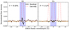 |
Fig. A.1. Stacked residual spectra normalized by emission-line flux for Hβ (left) and Hα (right). The black solid curves are the normalized residual spectra, while the red dashed curves are the normalized gas-only (i.e., stellar-continuum subtracted) spectra for reference. The orange horizontal lines denote where the flux is zero. The F values (upper-left corners) indicate the fraction of integrated residual flux compared to the emission line flux, measured within the blue-shaded region of 20 Å width. |
Unfortunately, given that the “true” stellar templates of the observed spectra are unknown, direct comparison with the ones derived from the fitting involving “true” templates is impossible. Thanks to the complete DAP output, we here provide an indirect examination using the residual spectra after removing the best-fit models of both stellar continuum and emission lines. This calculation aims to check whether there is a significant nonzero flux on the residual spectrum at the location of Hα or Hβ line. We used the main sample (i.e., the S/N-selected star-forming sample) described in Section 2.2 and retrieved their residual spectra from the DAP output, which were then de-reshifted, resampled to the same wavelength grid, normalized by the measured fluxes of the lines we want to check (i.e., Hα or Hβ). The median spectra of these Hα- or Hβ-flux normalized residual spectra are exhibited in Fig. A.1. We also provide the median stacked spectra of the gas-only spectra (i.e., only removing the best-fit stellar continuum models from the observed spectra) for reference in the figure. We calculated the integrated fluxes over a wavelength window of 20 Å around the examined lines, which is large enough to enclose the lines (see the blue shaded region in Fig. A.1), resulting in fractional residual fluxes of 0.48% and 0.52% for Hβ and Hα, respectively. Such residual fluxes are much smaller than either the absolute or relative flux calibration of the MaNGA spectra (Yan et al. 2016b) and thus can be ignored.
On the other hand, to allow a direct comparison with the EW(Hβ) bias reported by Groves et al. (2012), we also computed the integrated residual fluxes normalized by the continuum level underneath the Hβ line for individual spaxels. The EWs of the residual fluxes give a median value of 0.04 Å, about one order of magnitude smaller than the value reported by Groves et al. (2012).
In short, besides what Belfiore et al. (2019) has demonstrated on the robustness of the emission line measurements using mock spectra, we provide empirical evidence using the residual spectra from data to show that both the stellar continuum and the Hα and Hβ lines are well modeled on average by the DAP. We thus believe that the flux measurements for Hα and Hβ should be statistically unbiased at least for our main sample.
Appendix B: Results for other recombination lines
In the main part of this paper, we only present and discuss the results for the Hγ, Hδ, P8, and P10 lines, here we further provide results for the remaining hydrogen recombination lines that were measured by the DAP. In Figures B.1 and B.2 we provide the comparisons between the observed and simulated line ratio plots and the best-fit results for high-order Balmer lines (i.e., H7, H8, H9, H10, H11, and H12) and P9, respectively. Note that the median curves and the density contours of the observations are different in Figures B.1 and B.2 since different samples (the S/Ncut = 3 sample and the ΣSFR, cor-selected sample, respectively) were used to generate these plots (see Section 4.3.2). The best-fit parameters of these lines for the fitting sample are also given in Table 1 for reference.
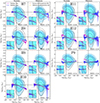 |
Fig. B.1. Similar to Fig. 3 but for other hydrogen recombination lines (i.e., H7, H8, H9, H10, H11, H12, and P9). |
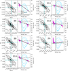 |
Fig. B.2. Similar to Fig. 7 but for other hydrogen recombination lines (i.e., H7, H8, H9, H10, H11, H12, and P9). |
Similar to what we observe in Fig. 3, the uncertainties of emission-line measurements exhibit prominent influences in the line ratio plots in terms of letting the median curves depart from the cross points predicted by the Case B recombination and scattering the line ratios to regimes that cannot be covered by the true values. When comparing the model predictions from the foreground screen and uniform mixture dust models with the observations, we can reach the same conclusion as Fig. 3. Namely, most of the spaxels favor the foreground screen model rather than the uniform mixture one for the high-order Balmer lines up to H12 and P9. We inspect further for the foreground screen case and find more details that reveal the problem in the data quality.
It seems that only the median curve of H7 can give a roughly consistent trend with the simulated one in terms of both slope and intercept. Although the difference in the intercept of the median curve between the observed and simulated (i.e., the predictions of the Case B recombination) samples of H7 are not as small as those of Hγ and Hδ, the best-fit c is very close to 1 (see Fig. B.2 and Table 1), indicating a < 1% correction for the model predicted fluxes. We thus believe that the slope of the attenuation curve at the wavelength of H7 can be well determined by our method.
For H8, the observed median curve has a large systematic offset from the simulated one, which should be primarily attributed to the influence from the nearby He Iλ3888 line. These two lines cannot be resolved from the MaNGA spectra, and thus their fluxes are very difficult to constrain via the DAP since no prior information about the fluxes is applied. From H9 to H12, all the observed median curves show deviations from the Case B predicted (simulated) ones to some extent. Similar results but for the ΣSFR, cor-selected sample can be found in Fig. B.2. The best-fit c parameter of these high-order Balmer lines for the fitting sample ranges from 0.55 to 0.84, suggesting that substantial corrections should be applied to fX, pre to match the observed fluxes.
Sources of such systematic corrections might be the improper subtraction of the stellar continuum since the flux measurements of these Balmer lines should be corrected for evident stellar absorptions that strongly depend on the stellar continuum modeling. If true, our finding might imply that the stellar models involved in the DAP continuum modeling still need to be improved to recover the stellar absorptions of the Balmer lines more accurately. Correcting for stellar absorption becomes more critical for these high-order Balmer lines compared to those with smaller upper atomic level n due to the dominant role of the stellar absorption over the nebular emission for these lines even for a very young stellar population (González Delgado et al. 1999). The weakness of these lines also implies that the zero-flux problem discussed in Section 4.5 should have a large impact on the scaling factor.
On the other hand, although we argue that the Case B recombination assumption works for the four lines we studied in the main text, departures from this assumption were also reported for some high-order recombination lines. Mesa-Delgado et al. (2009) observed enhanced intensities for both the Balmer and Paschen lines with an upper atomic level of n ≳ 13 compared to the Case B predictions in the Orion Nebula, while Domínguez-Guzmán et al. (2022) further argues that for H II regions in Magellanic Clouds, the deviations from the Case B values were found for recombination lines with n > 7. However, the observational evidence relies on the adopted dust extinction curve (also see Domínguez-Guzmán et al. 2022). Extinction-independent determination of the intrinsic intensities of these high-order lines for more H II regions is required to confirm such deviations. If exist, the elevated intrinsic fluxes would result in c > 1, which is in contrast with the best-fit results from H9 to H12 shown in Fig. B.2.
For P9, the observed median curve given in Fig. B.1 has a large upturn toward the low-Hα/Hβ end, which cannot be explained by the large uncertainties of emission-line measurements and implies a large overestimate of the P9 fluxes. Similar but less significant features have been observed for P8 and P10 displayed in Fig. 3. We attribute this feature to the residuals of night-sky lines. It seems that the P9 line suffers more contaminations from these residuals compared to P8 and P10, which is consistent with our experience of visual inspection of individual spectra of spaxels with the Paschen line detections. The upturn feature is much weaker for the ΣSFR, cor-selected sample for which the best-fit c is very close to 1, as shown in Fig. B.2. However, considering the influence of the sky residuals, we do not want to claim a good fitting for P9 in this work.
In principle, adding the scaling factor as a free parameter in the fitting could ensure that mX still can be well determined if the corrections to fX, pre exist but are systematic and independent of the physical properties (more specific, the Hα-to-Hβ ratio) of spaxels (e.g., a multiplicative systematic error of flux calibration). However, it is difficult to determine whether the main reason for the non-unity best-fit c varies with the Hα-to-Hβ ratio. Therefore, we claim that among these Balmer lines and P9, only H7 has a reliable fitting, and thus mH7 for the H II region-dominated spaxels can be well determined.
Appendix C: Proof of an unchanged slope when using different fiducial curve
The definition of mX (Equation 9) contains the attenuation difference between Hα and Hβ, which varies with the adopted extinction or attenuation curve. In Section 4.2 we claim that the best-fit mX should remain unchanged when using another fiducial curve in our fitting. To prove this statement, we here provide a brief derivation to demonstrate that for a given mX 10 and a set of emission-line observations fi,obs of one spaxel, our fitting approach, in principle, can return the same predicted flux fi,pre for Hβ and the targeted line and thus keep ln𝒫spaxel unchanged even when the attenuation difference AHβ − AHα varies with the adopted fiducial curve. Notably, the above two statements are equivalent.
We define a total-to-select attenuation between Hα and any other recombination line X as
 (C.1)
(C.1)
then the relative slope mX can be rewritten as
 (C.2)
(C.2)
Assume that for a given Rαβ and RαX (thus a fixed mX), the spaxel has a best-fit solution (fHα, int, AHα) that lets lnℒspaxel reach its maximum lnℒspaxel, max. Below we show that if both Rαβ and RαX are both scaled by a constant 𝒞 (i.e., mX remains unchanged), a new  could let the lnℒspaxel, max unchanged (i.e., the model predicted fluxes fi,pre in Equation 12 are unchanged). For Hα, requiring the predicted fluxes to be the same gives
 (C.3)
(C.3)
thus the intrinsic Hα flux after the scaling should be  . Assume that the intrinsic line ratio between the recombination line X and Hα is rint, Xα, then the intrinsic flux of X after the scaling can be written as
 (C.4)
(C.4)
in which fX, int is the intrinsic flux of X before the scaling. Because RαX is scaled by 𝒞, we have  from which the new dust attenuation for line X can be obtained via
  . The predicted flux for line X after the scaling is
![Mathematical equation: $$ \begin{aligned} f^{\prime }_{\rm X, pre}&=f^{\prime }_{\rm X, int} 10^{-0.4A^{\prime }_{\rm X}} \nonumber \\&=f_{\rm X, int} 10^{0.4(\mathcal{C} -1)A_{\rm H\alpha }}\times 10^{-0.4[A_{\rm X}+(\mathcal{C} -1)A_{\rm H\alpha }]}\end{aligned} $$](/articles/aa/full_html/2024/11/aa51339-24/aa51339-24-eq26.gif) (C.5)
(C.5)
 (C.6)
(C.6)
thus  . In other words, the predicted flux for line X remains unchanged after scaling RαX by a constant. Since line X can be any hydrogen recombination lines other than Hα, the relation between mX and RαX (Equation C.2) further implies that for a given mX, a new best-fit solution (
 ,
,  ) = (fHα, int100.4(𝒞 − 1)AHα, 𝒞AHα) can return the same ln𝒫spaxel, max if both Rαβ and RαX are scaled by a constant 𝒞. Therefore, using another fiducial curve only changes Rαβ, but the best-fit mX derived from our fitting method could remain in principle.
All Tables
All Figures
|
Fig. 2. Comparisons between the predictions from two geometry models and the observed fHα/fHβ–fX/fHα line ratios for Hγ, Hδ, P8, and P10. The magenta curves and shaded regions indicate the medians and their 3σ uncertainties of the binned distributions, respectively. In each panel, the red dashed line denotes the predicted relation based on the foreground screen dust model, while the orange dotted line is the prediction based on the uniform mixture model. The Fitzpatrick (1999) dust extinction curve with RV = 3.1 is assumed in both cases. The background gray map shows the logarithmic number density of our sample, while the cyan contours enclose 68%, 95%, and 99% of the H II region spaxels, respectively. The horizontal and vertical black lines indicate the intrinsic values of the corresponding ratios based on the Case B recombination. The median uncertainties of the sample are given in the lower-right corner. A close-up of the region around the cross point of the intrinsic line ratios is shown in the lower-left inset of each panel. |
| In the text | |
|
Fig. 3. Comparisons of the line ratio plots between the observations and the simulated samples generated by assuming the foreground screen dust model (left) and the uniform mixture model (right). In each panel, the filled contours and black contour lines indicate the spaxel distributions of the observed and simulated samples, respectively, both of which enclose 68%, 95%, and 99% of the corresponding samples from inner to outer. The magenta (blue) curve and shaded regions denote the medians and their 3σ uncertainties for the observed (simulated) sample, respectively. Regions around the cross points of the intrinsic line ratios are zoomed in and shown in the lower-left insets. The SSIM index describing the similarity in density distribution between the observed and simulated data is listed in the lower-right corner of each panel. Other symbols are the same as those in Fig. 2. |
| In the text | |
|
Fig. 4. Differences between the recovered and true values of the free parameters Δm (left) and c (right) as a function of the adopted Hα and Hβ S/N thresholds ranging from 3 to 100. Results based on the simulated catalogs with different true Δm are delineated by different colors. The fitting procedure to derive the best-fit parameters only includes the minimize step for saving computing resources. |
| In the text | |
|
Fig. 5. S/N of Hβ as a function of the corrected SFR surface density. The vertical red dashed line indicates S/NHβ = 50, while the blue dashed line is the selection criterion of H II region-dominated spaxels for the MaNGA survey proposed by Zhang et al. (2017). The two green horizontal lines locate ΣSFR, cor = 0.01 and 0.1 M⊙yr−1kpc−2, respectively. The three percentages suggest the fractions of spaxels within each ΣSFR, cor bin. Spaxels between the green lines are adopted as the subsample to fit the slopes of the nebular dust attenuation curve. The underlying gray map and cyan contours are the same as those in Fig. 1. |
| In the text | |
|
Fig. 6. Differences between the true and recovered Δm (using the minimize step only) as a function of the true Δm for our ΣSFR, cor-selected sample. The symbols with error bars indicate the means and standard deviations of the best-fit parameters for the 10 simulated samples in each case, respectively. |
| In the text | |
|
Fig. 7. Best-fit results for the four main recombination lines derived from the minimization-MCMC fitting method. In each case, Panel (c) shows the posterior probability distribution of the two parameters, while Panels (a) and (d) are the marginalized distributions of individual parameters. The cyan solid lines in these panels locate the medians of the corresponding distributions, and the cyan dashed lines enclose the 16th-84th percentile ranges of the distributions. The fit-best results with 1σ uncertainties (i.e., the 16th-84th percentile ranges) for ΔmX and c are listed in Panel (c). Panel (b) gives the comparison between the best-fit relation (green line) and the observed median curve (magenta curve) on the line ratio plane. Other symbols are similar to those in Fig. 2 but for the ΣSFR, cor-selected sample. |
| In the text | |
|
Fig. 1. Distribution of the S/N-selected spaxels in the P1–P2 diagram. The black solid curve is the H II region selection function given by Ji & Yan (2020). The background grayscale map shows the number density distribution of all the S/N-selected spaxels, while the cyan contours enclose 68%, 95%, and 99% of the H II region spaxels only, respectively. The median uncertainties of the S/N-selected sample are given in the lower-right corner, while the dust attenuation vector indicating E(B − V) = 1 mag is shown in the upper-right corner. |
| In the text | |
|
Fig. A.1. Stacked residual spectra normalized by emission-line flux for Hβ (left) and Hα (right). The black solid curves are the normalized residual spectra, while the red dashed curves are the normalized gas-only (i.e., stellar-continuum subtracted) spectra for reference. The orange horizontal lines denote where the flux is zero. The F values (upper-left corners) indicate the fraction of integrated residual flux compared to the emission line flux, measured within the blue-shaded region of 20 Å width. |
| In the text | |
|
Fig. B.1. Similar to Fig. 3 but for other hydrogen recombination lines (i.e., H7, H8, H9, H10, H11, H12, and P9). |
| In the text | |
|
Fig. B.2. Similar to Fig. 7 but for other hydrogen recombination lines (i.e., H7, H8, H9, H10, H11, H12, and P9). |
| In the text | |
Current usage metrics show cumulative count of Article Views (full-text article views including HTML views, PDF and ePub downloads, according to the available data) and Abstracts Views on Vision4Press platform.
Data correspond to usage on the plateform after 2015. The current usage metrics is available 48-96 hours after online publication and is updated daily on week days.
Initial download of the metrics may take a while.