| Issue |
A&A
Volume 691, November 2024
|
|
|---|---|---|
| Article Number | A43 | |
| Number of page(s) | 19 | |
| Section | Interstellar and circumstellar matter | |
| DOI | https://doi.org/10.1051/0004-6361/202450842 | |
| Published online | 29 October 2024 | |
Running with the bulls
The frequency of star-disc encounters in the Taurus star-forming region
1
Université Côte d’Azur, Observatoire de la Côte d’Azur, CNRS, Laboratoire Lagrange,
06300
Nice,
France
2
Univ. Grenoble Alpes, CNRS, IPAG,
38000
Grenoble,
France
3
Astronomy Department, University of Michigan,
Ann Arbor,
MI
48109,
USA
4
Department of Astronomy, Xiamen University,
1 Zengcuoan West Road, Xiamen,
Fujian
361005,
China
5
Astronomy Department, University of California Berkeley,
Berkeley
CA
94720-3411,
USA
6
Dipartimento di Fisica “Aldo Pontremoli”, Universita degli Studi di Milano,
via Celoria 16,
Milano
20133,
Italy
7
Lund Observatory, Division of Astrophysics, Department of Physics, Lund University,
Box 43,
221 00
Lund,
Sweden
★ Corresponding author; This email address is being protected from spambots. You need JavaScript enabled to view it.
Received:
23
May
2024
Accepted:
19
September
2024
Abstract
Context. Stars and planets form in regions of enhanced stellar density, subjecting protoplanetary discs to gravitational perturbations from neighbouring stars. Observations in the Taurus star-forming region have uncovered evidence of at least three recent, star-disc encounters that have truncated discs (HV/DO Tau, RW Aurigae, and UX Tau), raising questions about the frequency of such events.
Aims. We aim to assess the probability of observing truncating star-disc encounters in Taurus.
Methods. We generated a physically motivated dynamical model including binaries and a spatial-kinematic substructure to follow the historical dynamical evolution of the Taurus star-forming region. We used this model to track star-disc encounters and the resulting outer disc truncation over the lifetime of Taurus.
Results. A quarter of discs are truncated below 30 au by dynamical encounters, but this truncation mostly occurs in binaries over the course of a few orbital periods, on a timescale ≲0.1 Myr. Nonetheless, some truncating encounters still occur up to the present age of Taurus. Strongly truncating encounters (ejecting ≳10 percent of the disc mass) occur at a rate ∼10 Myr−1, sufficient to explain the encounter between HV and DO Tau ∼0.1 Myr ago. If encounters that eject only ∼1 percent of the disc mass are responsible for RW Aurigae and UX Tau, then they are also expected with encounter rate Γenc ∼ 100–200 Myr−1. However, the observed sample of recent encounters is probably incomplete, since these examples occurred in systems that are not consistent with a random drawing from the mass function. One more observed example would statistically imply additional physics, such as replenishment of the outer disc material.
Conclusions. The marginal consistency of the frequency of observed recent star-disc encounters with theoretical expectations underlines the value of future large surveys searching for external structures associated with recent encounters. The outcome of such a survey offers a highly constraining, novel probe of protoplanetary disc physics.
Key words: planets and satellites: formation / protoplanetary disks / binaries: general / circumstellar matter / stars: formation
© The Authors 2024
 Open Access article, published by EDP Sciences, under the terms of the Creative Commons Attribution License (https://creativecommons.org/licenses/by/4.0), which permits unrestricted use, distribution, and reproduction in any medium, provided the original work is properly cited.
This article is published in open access under the Subscribe to Open model. This email address is being protected from spambots. You need JavaScript enabled to view it. to support open access publication.
1 Introduction
Planet formation proceeds in a ‘protoplanetary disc’ of dust and gas over a timescale of ~3 Myr (e.g. Haisch et al. 2001). During this time, nascent planetary systems typically inhabit star-forming regions with a local stellar density that far exceeds the average in the galactic neighbourhood (e.g. Lada & Lada 2003). Neighbouring stars in these regions can provide feedback on the planet formation process in a variety of ways. These may include: external irradiation driving thermal winds (Winter & Haworth 2022, and references therein), chemical enrichment (Bastian et al. 2013; Lichtenberg et al. 2016; Parker & Schoettler 2023), late-stage gas infall (Dullemond et al. 2019; Kuffmeier et al. 2020, 2021, 2023) and star-disc encounters (Cuello et al. 2019, 2020, 2023). While all of these processes are of great interest for understanding the diversity of the observed exoplanet population, in this work we focus on the latter phenomenon. ‘Star-disc encounters’ refer to gravitational perturbations experienced by a protoplanetary disc during the close passage of a neighbouring star.
Various phenomena such as stellar accretion outbursts (Pfalzner 2008; Forgan & Rice 2010; Vorobyov et al. 2021; Dong et al. 2022) and spiral arms in protoplanetary discs (e.g. De Rosa & Kalas 2019) and free-floating planets (e.g. Vorobyov et al. 2017) – possibly including enigmatic binary planet-mass objects in the Orion Nebula cluster (Pearson & McCaughrean 2023; Wang et al. 2024; Portegies Zwart & Hochart 2023) – may all be feasibly attributed to stellar encounters. There remain alternative explanations; for example, spiral arms may be produced by gravitational instability (e.g. Douglas et al. 2013; Meru et al. 2017; Baehr & Zhu 2021) or (sub-)stellar companions (e.g. Dong et al. 2015; Ren et al. 2020). A search for flyby candidates that may have generated spiral arms by Shuai et al. (2022) revealed no evidence that nearby stars recently had a sufficiently close approach. However, such an effort is challenging due to proper motion uncertainties and the incompleteness of reliable measurements, particularly if a perturber is very low mass or is itself a binary. To assess the role of star-disc encounters for protoplan-etary disc evolution, we must estimate the rate of encounters in dynamically evolving star-forming regions.
The rate of stellar encounters, and their role for planet formation, is dependent on the local stellar density of the star-forming region. The stellar mass density ρ*. of star-forming regions can vary dramatically in the range 1 M⊙ pc−3 < ρ* < 106 ≲⊙ pc−3. The latter limit represents the most extreme stellar densities in the galaxy, such as in the cores of globular clusters that remain bound for a Hubble time (e.g. Krumholz et al. 2019). Intermediate densities ρ* ~ 103M⊙ pc−3 are typical in the cores of open clusters that may survive against galactic tides over 100 Myr or gigayear timescales. However, possibly the most common environments in which stars and planets form are the low density regions that produce loose ‘associations’, which are globally unbound against galactic tides. The average density in such regions has been assumed to be too low to induce frequent tidal encounters throughout the disc lifetime (e.g. Winter et al. 2018c).
Taurus is an example of a (globally) low density region, which does however host convincing evidence of at least three recent close star-disc encounters. These cases are RW Aurigae (Cabrit et al. 2006; Dai et al. 2015; Rodriguez et al. 2018), HV and DO Tau (Howard et al. 2013; Winter et al. 2018a), and UX Tau (Zapata et al. 2020; Ménard et al. 2020). Each of these systems exhibits a significant external structure that appears to be explained by recent flybys, sufficiently close such that they were capable of unbinding disc material. In an unstructured star-forming region at the average density of Taurus, the probability of a one-off random encounter over the disc lifetime is vanish-ingly small. This puzzle may appear to be partially resolved for some cases if the system is bound, such that close encounters occur periodically over the binary orbit. However, in isolation this is not a sufficient explanation. While repeated encounters in a multiple system can drive spiral arms in the disc (e.g. Alaguero et al. 2024), the disc should also be rapidly truncated such that on subsequent close approaches the gravitational pertu-bation no longer produces large extended tidal tails (e.g. Ménard et al. 2020). It is therefore necessary to perturb star-disc systems in Taurus stochastically, and do so over its ~1–3 Myr lifetime. In this manuscript, we aim to answer the question: do we expect sufficient star-disc encounters in Taurus to explain the frequency of observed recent encounters?
The role of stellar encounters has been the focus of numerous studies focusing both on the evolution of protoplanetary discs (e.g. Clarke & Pringle 1993; Ostriker 1994; Pfalzner et al. 2005; Winter et al. 2018b) and mature planetary systems (e.g. Spurzem et al. 2009; Shara et al. 2016; Winter et al. 2022; Li et al. 2024). Studies using N-body simulations often perform parameter studies or implement scaling relations to model star-forming regions. For example, one approach is to adopt the putative mass-radius (e.g. total stellar mass Mc and half-mass radius Rc) relationship for star-forming regions (e.g.  – Adams et al. 2006). However, the nature of this relationship varies depending on the sample and the definition of the mass and radius (Pfalzner & Govind 2021), and exhibits significant scatter. Mature and massive star clusters also do not appear to follow this relationship (Krumholz et al. 2019), and particularly for low mass or density regions it is challenging to unambiguously define an individual star-forming region. In addition, even within a well-defined ‘individual’ star-forming region, the internal structure has been shown to have a strong influence on the role of encounters (e.g. Craig & Krumholz 2013; Parker 2023). Assessing encounter rates therefore requires quantitatively matching the present day position-velocity structure. Yet it is not clear how well the widely adopted method for generating fractal initial conditions, sampling hierarchical boxes (Craig & Krumholz 2013), reproduces the observed spatial and kinematic structure in star-forming regions.
The structure of giant molecular clouds is set by turbulent fragmentation, from which the power-spectrum and Mach number determine the mass density distribution (e.g. Vazquez-Semadeni 1994; Padoan et al. 1997). An ideal approach to studying the role of dynamical encounters in young star-forming regions is therefore to model the star formation process directly through hydrodynamic simulations. Such simulations have shown that encounters are common during early disc evolution, possibly determining the initial distribution of pro-toplanetary disc radii (Bate 2018). However, these experiments are computationally expensive, following star formation only for ~0.1 Myr timescales. This makes parameter studies or tailored modelling of individual star-forming regions in this way impracticable.
Here we present a complementary approach to the above works, targeted at generating N-body initial conditions tailored to match young star-forming regions. We achieved this by simulating a Taurus-like star-forming region, with physically and empirically motivated initial conditions, including binaries. We drew stellar positions and velocities from an empirically constrained power spectrum, reflecting how turbulent energy is distributed across different scales. Our main aim has been to develop a dynamical model to track the history of stellar encounters in the Taurus star-forming regions. In doing so, we assessed whether the rate of disc-truncating star-disc encounters in Taurus is sufficient to produce the three known examples: HV/DO Tau, RW Aurigae, and UX Tau. This goal required ensuring that our dynamical model closely reproduces the present day spatial and kinematic structure in Taurus. We therefore review these structural properties in Section 2, which we used to benchmark our dynamical model. We discuss our approach for initialising initial conditions and dynamically evolving the model in Section 3, in which we also draw comparisons with the structure metrics introduced in Section 2. We discuss the rate of truncating encounters over time in our simulation in Section 4, quantifying the degree to which the observed examples of recent star-disc encounters are statistically expected. We summarise our conclusions in Section 5.
2 Properties of the Taurus star-forming region
2.1 Aim
An empirically motivated dynamical model for Taurus requires accurately quantifying kinematic substructure. If we had arbitrarily accurate and complete data for the 3D positions and velocities of all the stars in Taurus, then it would be trivial to use these data to generate N-body initial conditions to compute the future evolution of Taurus. However, as discussed in Section 2.2, while we have a fairly complete census of stars in terms of their projected spatial distribution, kinematic data is far more limited. Given the effects of multiplicity and extinction, parallax measurements also typically have associated uncertainties that make them impractical for use in setting initial conditions. In addition, we are interested in quantifying the frequency of encounters in the past, while we do not have direct measurements of the early spatial-kinematic stellar configuration in Taurus. For these reasons, we require metrics that characterise kinematic substructure. These metrics both guide our choice of initial conditions and offer a benchmark comparison for our models.
In the following, we first review the data for the stellar population in Taurus (Section 2.2). We then discuss how we quantified spatial structure in Section 2.3 and kinematic structure in Section 2.4.
2.2 Data
We used the census of Taurus members by Luhman (2023), with astrometric data from Gaia DR3 (Gaia Collaboration 2016, 2023; Babusiaux et al. 2023). This catalogue contains 532 members, with a high degree of completeness for spectral types earlier than M6-M7. When we considered proper motion differences between neighbours (Section 2.4), we restricted the sample to the 271 that have a reliable astrometric solution by the canonical criteria that the Renormalised Unit Weight Error (RUWE1) is smaller than 1.4 in Gaia DR3.
We cannot use the observed 3D positions directly to generate initial conditions for several reasons. Most obviously, the sample for which we have parallax is incomplete (417/532), and the typical uncertainties on the parallax correspond to a few pc. This means that small scale structure is not resolvable along the line-of-sight. We therefore generate our initial conditions parametrically, closely comparing with the observed structure in Taurus. We consider only the projected separations between stars when inferring the spatial and velocity structure of the region.
2.3 Spatial substructure
We aim to understand the role of close neighbours on disc evolution. A sensible metric to quantify structure is therefore the normalised pair separation function, which can be defined in two dimensions  . This is the averaged surface density of neighbours for any given star, normalised to unity when integrated over 2π∆R d∆R. This surface density evolves over time, and we therefore used this metric to ensure that we captured the time at which the dynamical state in our simulation is similar to that in Taurus.
Two related but complementary metrics are the one- and two-point correlation functions, Ψ(∆R) and ξ(∆R) respectively. These metrics have been applied by Joncour et al. (2017) and Joncour et al. (2018) to study the structure in Taurus. They are broadly defined as the excess of pairs with a given separation compared to a random, uniformly distributed population of stars in the same area. The one-point correlation Ψ is an excess of nearest pairs, while the two-point correlation represents the excess of all pairs. Of particular relevance for this work, Joncour et al. (2017) applied the one-point correlation function to demonstrate that approximately 40 percent of stars in Taurus are in ultra-wide binaries, with separations in the range 1.6 × 10³−5 × 10⁴ au. We used this inference to motivate our initial conditions, and the one- and two-point correlation functions to validate our model a posteriori. In particular, from the one-point correlation function Joncour et al. (2017) find a region of ‘inhibition’ (a smaller number of pairs than expected from random sampling) between ~0.1 and ~0.5°, while up to ~0.2°, Ψ ∝ ∆R−1.5. For the two-point correlation function, ξ > 1 out to ∆R ≈ 2°.
2.4 Velocity substructure
Stellar velocities are inherited from the velocities of the material from which they form, and are thus dependent on the kinematic structure of the parental molecular cloud. This velocity structure in a turbulent medium is driven by interacting waves that generate an energy cascade that is described by an energy spectrum E(k). Across a wide range of length scales λ, it can be approximated by a power-law (e.g. Elmegreen & Scalo 2004):
 (1)
(1)
where P(k) is the (three dimensional) power-spectrum, k is the wavenumber, συ,k is the characteristic velocity for k.
A range of β values in the interstellar medium (ISM) have been inferred observationally. These range from the original estimate for the size-linewidth relation for molecular clouds yielding β ≈ 1.76 (Larson 1981) to larger β ≈ 2.3 (Münch 1958; Heyer & Brunt 2004, for example). For weakly compressible turbulence, the energy spectrum for density and velocity follow the same power-law. Qian et al. (2018) find β ≈ 2 on small scales <2 pc (suggestive of compressible turbulence) and β ≈ 5/3 in the range ~5–10 pc (suggestive of incompressible turbulence, see also Brunt 2010). Ha et al. (2022) estimated β ≈ 1.7 from the stellar population and β ≈ 1.8 from Hα, both on ~10 pc scales.
For our purposes we adopted β = 2, appropriate for supersonic, rapidly cooling turbulence (Burgers 1948). Fhe velocity dispersion relation we adopted is then:
 (2)
(2)
where we chose normalisation constants συ,0 = 0.6 km s−1 for ∆r0 = 1 pc. Fhis yields a velocity dispersion similar to that empirically inferred for the youngest stars on galactic scales in the solar neighbourhood (e.g. Holmberg et al. 2009), while more importantly matching the dispersion in Faurus down to binary length scales. In Figure 1, we show the distribution of proper motion differences for nearest neighbours as a function of their separation in Taurus. We also show the Maxwell-Boltzmann distribution:
 (3)
(3)
in two dimensions (ND = 2) for Equation (2) with a Keplerian component appropriate for a star of mass m* = 0.5 M⊙ added in quadrature. This shows that the majority of neighbours follow the expected separation-velocity relation. Neighbours with a much larger relative velocity may have larger physical than projected separations. We applied the size-velocity relation given by Equation (2) to generate stellar velocities, and compared the appropriate Maxwell-Boltzmann distribution to the nearest neighbour relative velocities we generate in our model, both initially and after dynamical evolution.
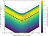 |
Fig. 1 Proper motion difference as a function of angular separation on the plane of the sky for nearest neighbours in the Luhman (2023) sample for Taurus. Red data points are the observed sample, with uncertainties propagated from Gaia uncertainties. The black line shows the velocity dispersion as a function of separation we adopt for our model, with a Keplerian component that dominates at small separations. The transition between the two power-laws is the break between the binary and individual systems (~5 × 10⁴ au, comparable to the galactic tidal radius for typical stars). The colour bar shows the corresponding Maxwell-Boltzmann distribution, normalised for each separation. See text for details. |
3 Numerical method
3.1 Overview
Our approach for simulating a Taurus-like star-forming region was to use a physically and empirically motivated set of initial conditions, including binary systems. We then benchmarked our model against the spatial-kinematic properties of the present day Taurus to ensure that the simulation reflects the observed dynamical state. With this model, we were able to extract encounters that we converted into the protoplanetary disc radii evolution using analytic formulae fit to numerical experiments (Winter et al. 2018c).
In the remainder of this section, we detail this process. First, we discuss our method for generating physically motivated initial conditions, starting with a gas density distribution in Section 3.3, which we converted to a stellar density distribution following the approach in Section 3.4. We then discuss implementing empirically motivated binaries in Section 3.6 and the appropriate velocity substructure in Section 3.8. We validated our dynamical model with respect to the observed dynamical state in Taurus as described in Section 3.9. Finally, we discuss our approach for extracting close stellar encounters from the simulation in Section 3.10 and the resultant disc evolution in Section 3.11.
3.2 Nbody code
Throughout this work, we used NBODY6++ (Aarseth 2003; Spurzem 1999; Wang et al. 2015) to integrate the stars and binary systems under gravity for 3 Myr. Given our interest in the short term evolution of a low mass star-forming region, we did not include stellar evolution. Nor did we include tidal binary circu-larisation, or an external potential. To capture the role of several neighbours, we insisted on a short time-step factor for the irregular force polynomial 5 × 10⁻³. The parameter adjustment time in N-body units is 10−4 in code time-units that are 3.22 Myr, at which the régularisation parameters are updated. The parameter and initial condition file for our fiducial model are available online2.
3.3 Log normal gas density field
We aim to initially generate a physically motivated gas density distribution, from which to draw our stellar population. Numerical experiments have shown that the mass density p of isothermal turbulent flows is well approximated by a lognormal distribution (e.g. Vazquez-Semadeni 1994; Nordlund & Padoan 1999; Ostriker et al. 1999). In order to generate a lognormal gas distribution, we first needed to generate a Gaussian density field over a 3D grid. Generating a density field that we could use to produce initial conditions for the N-body simulation is not trivial, since a Gaussian random field may exhibit peaks close to the edges of the grid. These peaks would be the site of high stellar density (or ‘NESTS’ – Joncour et al. 2018), and may be partially excluded by the grid. Indeed, the centre of the grid can represent a ‘void’ (underdensity) in the Gaussian field, which would undermine our goal to explore the interactions between stars in overdensities. Since we also needed a grid that covers a large dynamical range (from the size scale of Taurus, down to the wide-binary scale), it is not practicable to simply choose a subset of the complete Gaussian random field with a very high resolution. It is therefore useful to apply an approach that ensures that we can centre the grid on an overdensity.
While we could have attempted to do this by multiplying the density field by a centrally concentrated profile (such as a 3D Gaussian or Plummer profile), this would fundamentally change the nature of the density field and corresponding power spectrum. To avoid this we adopted a two-stage process, inspired by cosmological zoom-in simulations and applying the publicly available GENETIC3 code (Stopyra et al. 2020, 2021). This code generates a zoom-in or splice (Cadiou et al. 2021) self-consistently within a surrounding Gaussian random field by Fourier-space filtering. The net effect is that we were able to generate an initial, coarse Gaussian field, and then zoom in on an overdensity that represents the centre of our model for Taurus.
Our approach for this is represented graphically in Figure 2. We first generated a Gaussian random field over a 2563 grid with side length 100 pc. We adopted a power spectrum index of −3. We did not quantitatively fit for this index, but select a posteriori between indices −2, −2.5, −3 and −4, finding that −3 reproduces a stellar density structure that matches the observed structure. Empirically, this index is comparable to that inferred in Taurus by Brunt (2010).
From the large scale density field, we located local maxima over 5 pc length scales using the ndimage.maximum_filter algorithm from SCIPY (Virtanen et al. 2020). We chose the 20 greatest local maxima and selected the closest to the centre of the grid, ensuring the zoom-in grid will be within the range of the initial grid. We then used GENETIC to generate a new Gaussian density field on a grid that is smaller by a factor three (a box side length of 33 pc), with 10243 grid cells. This defines a field which has a high density centre, and a resolution of 0.032 pc, or ~7000 au, down to length scales comparable to wide binary separations. Finally, we enforced a dispersion  on the logarithmic density field. This is approximately the expected dispersion given a sound speed cs = 0.2 km s−1 and the root mean square velocity
  for ∆r ~ 30 pc, according to Equation (2).
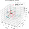 |
Fig. 2 Illustration of how we selected a box from which to generate a lognormal density field from a larger-scale, low resolution lognormal density field. We illustrate the underlying density grid by drawing faint black points with density proportional to the local density field. Cyan points indicate our selection of the top 20 density maxima from the density field. The red star indicates the position of the adopted box centre. The dashed red lines indicate the boundary of the new zoom-in box. |
3.4 Stellar spatial distribution
We next drew a stellar spatial distribution from our underlying gas density profile. To do this, it was necessary to consider which regions of the cloud are able to rapidly collapse to form stars. The relevant timescale for this collapse from rest is the free-fall timescale:
 (4)
(4)
To infer a free-fall time across our grid, we required an absolute density scale, for which we assume a total mass within the box of 104 M⊙, corresponding to the approximate total gas mass in the Taurus complex (Goldsmith et al. 2008). We then imposed a constraint that grid cells must have τff < 1 Myr in order to host a star, comparable to the empirical age dispersion Luhman (2023). We assigned probabilities to these grid cells  – that is, the probability of forming a star is proportional to the quantity of material multiplied by the rate at which that material is expected to collapse. For a selected grid cell, we then offset the location of the formed star such that it was placed randomly within the cell. We validated this choice of spatial distribution in our dynamical model a posteriori, as presented in Section 3.9.
For the total number of systems, we drew Nsys that yields a total number of stars N* that is broadly consistent with the findings of Luhman (2023). This is not trivial, both because there is not a clear detection limit for that sample and because we include binaries stochastically from the initial population of potential primaries, as well as the ultrawide binary fraction inferred by Joncour et al. (2017). Further, it is not clear what fraction of binaries are resolved/detected by Luhman (2023). We perform a two stage process as follows in Sections 3.5 and 3.6.
3.5 Ultrawide pairs
First of all, we corrected the total number of stars for a given fraction of ultrawide binaries 𝓕uwb = 2/3. We consider 400(1 – 𝓕uwb/2) = 267 stars with masses > 0.08 M⊙ (half of these would end up in ultrawide binaries). We then added the fraction of brown dwarfs we expect below this limit from the initial mass function (IMF). For this, we used the following IMF (e.g. Kroupa 2001):
 (5)
(5)
with normalisation constants such that ξ is continuous and integrates to unity over all m*. For each of these stars, we then drew an ultrawide companion with a total probability 𝓕uwb. This yielded 660 stars and sub-stellar objects in total, 38 percent of which with masses <0.08 M⊙. We then drew the masses of all stars from Equation (5).
The ultrawide pair fraction we adopted is somewhat higher than 𝓕uwb ≈ 0.55, inferred by Joncour et al. (2017); 186 of the 338 stars in their sample are in ultrawide pairs. However, some of these companions separate during dynamic evolution. We also note that Joncour et al. (2017) found evidence that members of ultrawide pairs are ~15 percent more likely to be themselves in a shorter period binary. However, given that this is a relatively minor correction to the binary fraction, and it is challenging to disentangle dynamical versus primordial origins for these statistics, we did not include this enhancement. While we do not forward model the initial fraction, we validated our choice by comparing the one-point correlation function in our model with that computed by Joncour et al. (2017) in Section 3.9.
The separations for the ultrawide pairs is approximately loguniform between 1.6 × 10³ au and 5 × 10⁴ au (see Fig. 7 of Joncour et al. 2017), and we therefore drew semi-major axes of these companions similarly. We assumed a uniform eccentricity distribution up to 0.9, and a random orientation (as described in Section 3.6).
3.6 Binaries
We defined binaries separately from ‘ultrawide pairs’, described above and treated as single stars in terms of their mass-function. We considered the entire population of stars (including each member of the ultrawide pairs) to be potential primary stars in a binary system, and added companions to a subset.
The binary population we included is empirically motivated, based on the findings of Moe & Di Stefano (2017). In brief, we used the same functional form for the probability of each primary having a companion in each dex of orbital period space, modified in a number of ways. Firstly, we excluded binaries with period P < 105 days (≲30 au); such binaries are close enough to be largely uninfluenced by encounters, and in the context of proto-planetary discs may host circumbinary discs. At longer periods, we removed the exponential taper that Moe & Di Stefano (2017) infers for P > 105.5 days, instead assuming a constant binary fraction per dex out to P = 107.7 days, approximately corresponding to the scale at which we transition to ultrawide binaries. The log-uniform distribution is consistent with the observed separations for the ultrawide pairs (see Fig. 7 of Joncour et al. 2017), and for wide binaries in the field (Lépine & Bongiorno 2007). For all binaries, we drew eccentricities uniformly from 0−0.9 (e.g Abt 2006, and review by Duchêne & Kraus 2013).
Once we had randomly drawn the periods and eccentricities for the companions of our initial population, we drew the mass ratio. For the ultrawide binaries, we drew masses from the IMF, as described in Section 3.4. For the regular binaries, we drew mass ratios q in the range 0.1 < q < 1 from a probability density function p(q). To construct p, we defined two power-law regime with indices γsmall for q < 0.3 and γlarge for q ≥ 0.3. Following Moe & Di Stefano (2017), we also included an excess probability of the star having a twin, where a twin is defined as having a mass ratio 1 – ∆twin < q ≤ 1. This is defined in practice by computing the quantity:
 (6)
(6)
where
 (7)
(7)
Then finally the probability density function for q is:
 (8)
(8)
Since we only considered P > 105 days and largely low mass stars, we have only two regimes for the power-law indices. For P < 106 days we have γsmall = 0.4 and γlarge = −0.4, and otherwise we have γsmall = 0.5 and γlarge = -1.1. We fix 𝓕twin = 0.1, for ∆twin = 0.05. These values are consistent with observational constraints, although typical uncertainties are high for many of these values (El-Badry et al. 2019). When we generated our initial population, we also excluded any companions that are generated that have masses below our lower IMF limit (0.01 M⊙), although in practice this only influences brown dwarf primaries. The overall binary fraction is ~30 percent for binaries with orbital periods >105 days, which is broadly consistent with the field population (e.g. Niu et al. 2021). We show the statistics of our binary and ultrawide pair distribution for the stellar population in Figure 3.
Finally, we generated the positions and velocities of the companion population by randomly sampling cos i (for inclination i), the argument of periapsis, longitude of ascending node and true anomaly uniformly over the appropriate ranges. We then computed the appropriate position and velocity vector of the companion with respect to the primary. We thus produced the initial binary population that we evolve dynamically during our simulation.
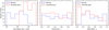 |
Fig. 3 Histogram showing the distribution of companions at a given semi-major axis (left) eccentricity (middle) and mass ratio (right) for primary stars with masses m* > 0.08 M⊙. The red histogram is for those pairs we define as ultrawide pairs, while the blue shows the binaries. |
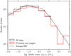 |
Fig. 4 Histogram of stellar masses in our dynamical model for Taurus. The solid black shows all stars including binary companions, while the red line is just the primaries and single stars. The black dashed line corresponds to the number that would be expected in each bin from the Kroupa (2001) IMF (Equation (5)). The bin sizes are similar to those adopted by Luhman (2004) in Figure 13, top panel. |
3.7 Mass function
We have already described our stellar mass drawing procedure for single stars and binaries in Sections 3.5 and 3.6. To validate our mass distribution including the binary population, we show the histogram of stellar masses in Figure 4. The bins used for this histogram are similar to those used by Luhman (2004, top panel of their Figure 13). The number of approximately solar mass stars found by Luhman (2004) is ~40. This number is close to complete for Taurus, and is similar to our drawing from the IMF. More recently, Esplin & Luhman (2019) found a peak around m* ~ 0.15 and ~25 stars with m* ≳ 1M0 across the whole of Taurus, again comparable to our IMF draw. The mass function for all the stars, including binary companions, is shown as the black histogram in Figure 4. Despite including a different mass function for companions, the mass function is not greatly altered from the Kroupa (2001) IMF we initially assume for the primary population. We therefore conclude that we have drawn a similar stellar population to that of Taurus.
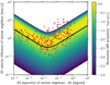 |
Fig. 5 Proper motion difference versus angular separation assuming a distance of 140 pc for nearest neighbours from the initial conditions in our model. The black line shows the one dimensional velocity dispersion as a function of separation and the colour bar shows the normalised Maxwell-Boltzmann distribution for each separation, as in Figure 1. |
3.8 Initial velocities
We assigned velocities to the primary stars we have generated motivated by our discussion in Section 2.4. We tackled this by generating velocities following a Gaussian process, such that velocities of stars that are close to each other are more highly correlated than those of stars at large separations. If ∆r < ∆rmax, we the corresponding kernel or covariance function is (e.g. see Equation (2.19) of Rasmussen & Williams 2006):
 (9)
(9)
where σv,max = σv(∆rmax). By this definition, the covariance function is not well defined for large ∆r > ∆rmax, where k becomes negative. However, we are free to choose an arbitrary large ∆rmax. In this case, we can rewrite the covariance function:
 (10)
(10)
where we have defined:
![Mathematical equation: ${{\cal D}_r} = {\left[ {1 - \exp \left( { - {{\Delta r} \over {\Delta {r_{\max }}}}} \right)} \right]^{0.5}}.$](/articles/aa/full_html/2024/11/aa50842-24/aa50842-24-eq16.png) (11)
(11)
Equations (9) and (10) are equivalent for large ∆rmax/∆r → ∞, but at large separations Equation (10) defines a maximal dispersion between stellar velocities. We chose Equation (10) because it yields well defined covariance for any ∆r. In practice, we anyway choose ∆rmax = 100 pc so that our choice is not important. In order to assign velocities given this kernel function, we defined the covariance matrix K = [kij] = [k(ri, rj)]. We then performed a Cholesky decomposition K = LLτ, where L is a lower triangular matrix. We defined a vector wα which is a vector with a length corresponding to the number of stars for which we assign velocities. We drew each wjα ~ 𝒩(0,1) independently for each spatial dimension α = d1,2,3. We then defined the velocity components for the stellar population uα = Lwα.
In Figure 5 we show the velocity difference between different nearest neighbours in our model initial conditions, including binaries. It is clear that our synthetic stellar population (scatter points) have relative velocities that follow a similar size-velocity relation, σv(∆r) as found in Section 2.4 – cf. Figure 1.
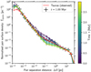 |
Fig. 6 Normalised pair surface density |

3.9 Model validation
We validated our model by analysing the structure metrics discussed in Section 2. First, we considered the pairwise separation distribution, as shown in Figure 6. The pair surface density profile  shows an excess at very small projected separations (∆R ≲ 5 × 10⁻⁴ pc), where the Luhman (2023) sample may be missing closer binaries. There is also a small excess around the binary transition at a few 10−2 pc. This excess is quickly lost as the system evolves, and the spatial structure is in good agreement with the observed population at ~ 1 Myr. We therefore adopted 1 Myr as the ‘present day’ in our simulation.
At this time, the velocity structure, illustrated in Figure 7, remains similar to the velocity structure we inferred in Taurus in Section 2.4. When comparing Figures 7 to 1, we note that there are some differences in how they are constructed. For example, close binaries are complete in our model, but not for those in Taurus. Indeed, in Taurus the sample is restricted to only stars with Gaia proper motions, with all the biases that implies. Nonetheless, the correlation between velocity and separation remains broadly similar. The transition in nearest neighbour velocity difference from ‘binary’ to ‘field’ coincides with the change in the power-law surface density profile in Figure 6 for ∆r ~ 3 × 10⁻² pc.
We also show the one- and two-point correlation functions in Figure 8. These can be compared directly to Fig. 4 of Joncour et al. (2017). We find a similar functional form for both, again indicating that the structure in our model matches the physical structure of Taurus. We find a very similar region of ‘inhibition’ in which Ψ < 1 in the range of separations 0.1 û 0.5°, and a similar power-law for Ψ where ∆R < 0.2°. We also recover ξ > 1 for ∆R ≲ 1°, close to the result of Joncour et al. (2017).
We conclude that our model, with initial conditions based on physical and empirical arguments, reproduces the observed dynamical state of Taurus at 1 Myr. The age in our model of 1 Myr is somewhat younger than the 1–3 Myr typically estimated for Taurus (e.g. Luhman 2023). If Taurus is typically older on average, this might suggest that the stellar distribution was initially more compact than the initial conditions in our simulation; although in this case we would also expect more rapid dynamical evolution. It is also possible that residual gas in the star-forming region slows down the dispersal of structure. However, then it would be plausible that discs in the high density regions are replenished by accretion of this residual gas (e.g. Kuffmeier et al. 2020), blurring the lines of what ‘t = 0’ means for disc evolution. In truth, probably a mixture of these influences, as well as a finite period of star formation, somewhat influence the dynamical evolution of the region. Nonetheless, for the purpose of this work, we are satisfied that the current state of stars and discs in Taurus is well approximated by our simulation at 1 Myr. In this context, we note that a posteriori we find that the frequency of strong encounters does not change rapidly between 1–3 Myr in our simulation (see Section 4.3).
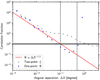 |
Fig. 8 One-point (Ψ, blue points) and two-point (ξ, grey points) correlation functions computed from our model at 1 Myr. The red line shows the Ψ ∝ ∆R−1.5 relationship for ∆R < 0.2° and the two dashed black lines enclose the region of inhibition (where Ψ < 1), as inferred by Joncour et al. (2017, see their Figure 4). |
3.10 Tracking encounters
Due partly to our inclusion of binaries, interactions between stars are too complex to be easily identified with a simple criterion ‘on the fly’ during the simulation. We therefore chose to analyse encounter properties by post-processing high frequency outputs. Specifically, we output 9299 snapshots from our simulation over 3 Myr, corresponding to a time step of 323 years. To accurately extract the correct encounter properties, we then performed the following analysis for each star i:
We identified the closest neighbour j(t) for each time step, spatially separated by vector ∆rij and with velocity difference ∆vij.
If the nearest neighbour j to i had a bound companion k which is separated from j by vector ∆rjk such that |∆rjk| < 0.1|∆rij|, we considered j and k to be a single star with the combined mass and momentum of j and k. In the following we refer to star j as the binary barycentre.
We searched for a sign change in the vector ∆rij ⋅ ∆vij from negative (approaching) to positive (receding). We define snapshot l, at time tl, for which |∆rij| is minimal between the two adjacent snapshots (l, l + 1).
We computed the analytic eccentricity e, closest approach distance rp, time of pericentre tp. If the predicted closest approach is not between tl and tl+1, then this must be a non-hierarchical multiple interaction, occurring on a short timescale (<323 years). In this case, we assumed that the closest approach is at tl (with closest approach distance given by the separation at this time), although in practice this is rare.
This procedure ensures that, despite the finite temporal resolution of our simulations, we were able to resolve the majority of encounters that are relevant to disc truncation. We limited the number of encounters to one per time step, thus we do not count every closest approach for close binaries which have an orbital period <323 years. Although we could in principle have included multiple encounters per time step, these encounters anyway quickly truncate the disc on short timescales. While our method may also not be accurate particularly for chaotic multiple interactions in cases where multiple interactions occur on timescales less than 323 years, we show in Appendix A that our results were not influenced if when we increased the output frequency.
3.11 Disc truncation and initial radii
To compute the post-encounter disc radius, we used the analytic functions inferred by Winter et al. (2018c). These functions were established by fitting a scale-free, angle-averaged expression to numerical test particle simulations, depending on the ratio of the closest approach distance rp to the outer disc radius Rout, the eccentricity of the encounter e and the mass ratio of the per-turber q. Since these fitting functions were inferred for unbound encounters, we will adopt e = 1 for encounters with e < 1 . We expect this to be a reasonable approximation. For example, Manara et al. (2019) fit an analytic functional form to the steady state truncation radius inferred from the numerical results of Artymowicz & Lubow (1994). For an equal mass system on a circular orbit, this estimate implies a truncation radius ~Rout ≈ 0.33 rp, which is the same as the steady state truncation radius implied by our prescription (see Figure 4 of Winter et al. 2018c). In practice, the majority of encounters that strongly truncate the disc at late times also have e ~ 1. We also consider all discs which experience encounters with rp < 10 au to be ‘destroyed’, making the assumption that the resultant compact disc may be rapidly accreted or photoevaporated (e.g. Clarke et al. 2001).
We initialised all discs with outer radii following (Andrews 2020):
 (12)
(12)
While this is empirically motivated by observed outer radii as inferred from CO emission lines, this relationship has a large scatter (which may in part be driven by dynamical truncation). The measurements themselves also come with numerous caveats originating from systematic uncertainties in outer radius definition, optical depth and chemistry (see e.g. Miotello et al. 2023). However, with these caveats we here assumed that the relationship is exact. We also did not consider viscous expansion (e.g. Lynden-Bell & Pringle 1974) or wind-driven contraction (e.g. Tabone et al. 2022). The discs therefore only evolved (shrank) as a result of star-disc encounters.
3.12 Caveats for the physical model
There are two main caveats for the dynamical model we present here. The first is that, while we are interested in establishing the rate of strongly disc-truncating interactions at a given system age, this depends on there being a well-defined age of the system at large. More specifically, we implicitly assumed that the spread in stellar ages is much smaller than the age of the system itself. This is almost certainly not the case, with the groups in Taurus having ages in the range ~1–3 Myr (Luhman 2023). However, our efforts are still valid in that a star-disc system will only undergo encounters with nearby neighbours, which we generally expect to have very similar ages. None of the existing examples of recent encounters have been suggested to be particularly young, but our conclusions can be reconsidered depending on the inferred ages of post-encounter systems.
The other major caveat is that we did not include the self-gravity of the ISM. Without including a fully hydrodynamical model, it is not possible to include this potential in a physical way. Our choice to ignore the gas potential is in a sense a similar assumption to the one discussed above, specifically that local star formation is completed instantly, and the gas is instantaneously dispersed (e.g. by stellar feedback). If instead a large quantity of residual gas remained within the individual star-forming regions that comprise the Taurus complex, then groups of stars may remain bound for longer. This may in turn increase the local encounter rate at later times. It is not possible to capture this gas potential without either full hydrodynamics (making matching exactly the structural properties of Taurus impossible), or by developing a scheme for integrating a complex potential that allows several components that co-move with stellar groups (beyond the scope of this work). However, we did find agreement between the dynamical state (i.e. correlation functions) in our model and observations, which would suggest the role of ISM self-gravity on the population dynamics as a whole cannot be dramatic. While this nonetheless remains a shortcoming of this work, we discuss in Section 4.5 that if high density gas alters our results this would have other interesting physical implications.
4 Results and discussion
4.1 Types of late-stage encounter
First, we qualitatively explored the nature of star-disc encounters in our simulation. For this we show some examples of encounters that occur at 1 ± 0.2 Myr in our simulation. The location of all these close encounters are shown in the central panel of Figure 9, from which we extracted the following categories:
- (a)
Stable, long period eccentric binary: possibly the most straightforward kind of encounter is a very long period binary which remains unperturbed by unbound stars, as shown in the top-left of Figure 9. This kind of encounter can still produce relatively large changes in outer disc radius if the orbital period is sufficiently long.
- (b)
Chaotic multiple: shown in the top-middle of Figure 9 is an example of a bound triple system that interacts to eventually eject one of the stars at ~0.8 Myr, leaving a tighter binary that can further truncate the disc.
- (c)
Perturbed eccentric binary: if a stable binary is perturbed by an encounter with an external (unbound) star, then this may also result in a tightening of the binary. A closer perias-tron distance can then further truncate the disc. We show an example of this in the top-right of Figure 9 (although in this case, the external star is in fact marginally bound).
- (d)
Random unbound encounters: this is the best-studied type of encounter, the rate of which can be understood analytically at a given local stellar density and velocity dispersion. However, in our simulation, we do not find any examples of random encounters. These encounters are more common in denser regions, but in Taurus we find that the majority of star-disc interactions are mediated by wide binary companions.
While this categorisation illuminates the value of physically motivated structure and multiplicity within models for star-forming regions, they are not rigid, and types of encounter may blur into each other. Our findings emphasise that unbound encounters and binary interactions cannot be studied separately during the dynamical evolution of a young star-forming region.
4.2 Disc evolution
We consider how encounters shape the global disc radius distribution in Taurus. This is illustrated in Figure 10, where we show the cumulative distribution of disc outer radii over the course of the simulation. We found that the vast majority of discs are rapidly truncated below their initial radius by encounters, and ~1/4 are truncated below 30 au. However, by the present time (1 Myr), dynamical encounters are not changing the overall distribution of disc radii significantly. This is because, while external perturbation does sculpt the outer disc for a large fraction of the population, disc truncation mostly occurs in stable binaries. Observations of discs in binary systems appear broadly consistent with theoretical expectations (Manara et al. 2019; Rota et al. 2022). We conclude that, for a region such as Taurus, the role of encounters for the disc population as a whole is largely dominated by early interactions in binaries, rather than an ongoing process of disc truncation.
4.3 Truncating encounter frequency
We now turn to the primary motivation of this work, and ask the question: do we expect sufficient close encounters in Taurus to produce the examples of recent dynamical interaction? To answer this question we require two definitions:
Which encounters produce significant external structures (e.g. tidal tails)?
For how long does this observable external structure persist? To answer these questions, we consider the rate of encounters that yield a fractional truncation −∆Rout/Rout above some threshold in the context of the observed flyby candidates in Taurus.
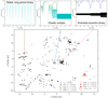 |
Fig. 9 Spatial distribution of stars (mass > 0.08 M⊙) at 1 Myr and contemporary disc-truncating encounters in our simulation. We show as coloured star or square symbols the location of all stars that underwent encounters yielding a fractional truncation −∆Rout/Rout > 0.01 over the age range 1 ± 0.2 Myr. Encounters that yielded −∆Rout/Rout > 0.1 are highlighted with red circles. In the panels along the top we show the separation between specific stars and their stellar neighbours over the first 1.5 Myr of the simulation. Each line represents the distance to a single stellar neighbour, linearly interpolated between snapshots, where neighbours that are one of the two closest stars at any given time step are included (if they pass within 104 au). In each plot, we mark the location of a logged ‘closest approach’ as a cross (inferred analytically from the closest time step – see Section 3.10). |
4.3.1 HV and DO Tau
The huge extended dust bridge between HV and DO Tau (Howard et al. 2013) appears to be the result of a strongly truncating encounter, possibly occurring during the dynamical decay of a quadruple system (Winter et al. 2018a). While the model of Winter et al. (2018a) is probably not a unique scenario for producing the observed structure, we can make some quantitative arguments as to the requirements of such an encounter. Assuming some grain growth occurred within the disc, the mass of material expelled during the encounter is Mex ~ 10−4 M⊙ (Winter et al. 2018a), which is ~10 percent of the current mass Mdisc of the disc around HV Tau C (Stapelfeldt et al. 2003). If the surface density of the disc ∑ ∝ R−1, for R the cylindrical radius inside Rout, this implies a fractional truncation −∆Rout/Rout ~ Mex/Mdisc ~ 0.1. To reach the present day projected separation of ≳104 au, the encounter must have occurred ~0.1 Myr ago. This would suggest a rate of ~10 encounters per Myr for encounters that result in a fractional truncation −∆Rout/Rout ≳ 0.1.
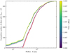 |
Fig. 10 Disc outer radius Rout evolution for the population of stars with m* > 0.08 M⊙ in our simulation. The colour bar shows the time at which the distribution is measured. The initial outer radius distribution is shown in red. |
4.3.2 RW Aurigae
For RW Aurigae, the best-fitting model explored by Dai et al. (2015) had an initial outer radius of 60 au and a final outer radius in the range ~40–57 au. This estimate is mostly based on the geometry of the spiral arm as inferred from their simplified radiative transfer. The 12CO emission detected around RW Aurigae is at least partly optically thick, so it is not possible to reliably infer a total mass that has been ejected in the encounter. The conclusions of Dai et al. (2015) may change if the apparent morphology as seen in CO differs when detailed chemistry, pho-todissociation or radiative transfer effects are taken into account. If the physical arm is longer and wider than they assume, the authors show that a weaker encounter can be consistent with the observed structure. Dai et al. (2015) also infer a time since closest approach ~600 years from their dynamical model. This conclusion may depend somewhat on the deprojected geometry of the spiral and the system orientation.
4.3.3 UX Tau
In the case of UX Tau, Ménard et al. (2020) focused on two different flyby simulations, with outer radius Rout = 60 au and 90 au, both with rp = 100 au, with a mass ratio of the per-turber q ~ 0.08–0.22. The former radius is close to the observed outer radius (post-encounter). Both simulations produce clear spiral arms and some extended structure, so a severely truncating encounter is not required. There are currently no estimates for the mass of the external structure with respect to the disc mass. From their simulations, Ménard et al. (2020) estimate ~1000 years since closest approach, with some margin for uncertainty in the system geometry as in the case of RW Aurigae.
4.3.4 Overall rates
The considerations above lead us to conclude that a small fraction of the disc mass may be capable of producing some of the observed external structures. We therefore explore a range of fractional truncation thresholds −∆Rout/Rout > 10−3, 10−2 and 10−1. Choosing a threshold smaller than 10-3 makes little difference to the overall encounter rate. As discussed above, ‘weak’ encounters with −∆Rout/Rout ~ 10−2 may be sufficient to reproduce the structures observed around RW Aurigae and UX Tau, while the stronger encounter threshold would correspond to systems like HV and DO Tau. While we cannot be confident of the exact −∆Rout/Rout that result in RW Aurigae and UX Tau-like systems, our results will motivate future studies quantifying the mass in the external structure surrounding systems that have undergone recent encounters, given that Mex/Mdisc ~ −∆Rout/Rout.
The overall encounter rate is summarised in Figure 11 for these thresholds. We binned the encounters by the time at which they occur and by their fractional disc truncation. We also show the evolution of individual discs by connected lines between individual encounters, so that the evolution of the outer disc radii in (for example) binary systems is clear. As expected from Section 4.2, the majority of discs are truncated rapidly in binary systems during the first ~0.1 Myr. However, there remain examples of individual encounters persisting throughout the course of the simulation. In order to explore the degree to which our results are stochastic, we ran two additional versions of our experiment described in Appendix B.
Quantitatively, we see that the rate of the strongest encounters −∆Rout/Rout > 0.1 remains at ~10 Myr−1 in the time range ~1 –3 Myr (see also Appendix B). Thus HV and DO Tau-like encounters, observable for ~0.1 Myr, are likely (probability ~50 percent) to be found somewhere in Taurus. We conclude that the occurrence of the HV and DO Tau encounter is expected in the context of our dynamical model.
The more recent RW Aurigae- and UX Tau-like encounters require a considerably higher encounter rate. The rate of weaker encounters −∆Rout/Rout > 10−2 is Γenc ~ 100 Myr−1, with approximately a factor order unity in stochastic variation (Appendix B). This rate is a factor~2–3 larger for −∆Rout/Rout > 10−3. We can write the probability of observing at least N encounters from a Poisson distribution:
 (13)
(13)
where τobs is the period for which the encounter is observable. Given that we are equally likely to observe the disc at any stage during this period of observability, this implies the average time of observation 〈tobs〉 = τobs/2. We therefore adopt a moderately generous τobs = 2000 years, a factor ~ 2 larger than the time since periastron for UX Tau and RW Aurigae. Taking a range of encounters Γenc = 100-200 Myr−1 for Nobs ≥ 2 (RW Aurigae and UX Tau) yields Pobs = 0.018–0.062. Therefore, if encounters with −∆Rout/Rout > 10−2 can produce these systems, then the tension with our model are not significant (or very marginally significant at ~2σ). If a much more truncating encounter is required, then this tension may become significant. This marginal agreement underlines the importance of future studies quantifying the fraction of mass in the extended structure.
In the absence of additional constraints, we conclude that the expected rate of encounters in Taurus is marginally sufficient to produce UX Tau and RW Aurigae without appealing to additional physics (see Section 4.5). However, this would not be the case if the sample of known recent, truncating star-disc encounters is incomplete. Indeed, there is some reason to suspect that this may be the case, as discussed below.
4.4 Masses of stars undergoing close encounters
We ask whether truncating encounters occur more or less frequently for high mass stars. We show the distribution of the masses of stars that undergo truncating encounters after 1 Myr in Figure 12. This mass distribution is indistinguishable to the overall mass function (m* > 0.08 M⊙). By contrast, RW Aurigae A and B have masses ~1.3–1.4 M⊙ and ~0.7–0.9 M⊙ respectively (Ghez et al. 1997; Woitas et al. 2001). HV Tau C has a mass ~0.5–1 M⊙ (Duchêne et al. 2010) and DO Tau ~0.3–0.7 M⊙ (Beckwith et al. 1990; Hartigan et al. 1995). UX Tau A has a mass ~ 1.3 M⊙ and UX Tau C has mass ~0.16 M⊙ (Kraus & Hillenbrand 2009; Zapata et al. 2020). The origin of the extended structures are the discs around RW Aurigae A, HV Tau C, DO Tau and UX Tau A. The masses of these stars appear to be systematically greater than what would be obtained from randomly sampling from the IMF. Assuming nominal masses of 1.4 M⊙, 0.8 M⊙, 0.5 M⊙ and 1.3 M⊙ for RW Aurigae A, HV Tau C, DO Tau UX Tau A respectively yields KS test p-value 0.023 percent when comparing to the stars that undergo encounters in our model. It is quite possible that observations could be biased to detect evidence of encounters involving more massive stars with brighter discs. However, this would imply many more undetected external structures that are evidence of encounters involving low mass stars in Taurus. Following Equation (13), if evidence for just one more encounter similar to RW Aurigae or UX Tau were uncovered in Taurus, this would being the 2σ encounter rate to Γenc ~ 680 Myr−1. Alternatively, this would yield Pobs ~ 10−3 even for weak encounters with Γenc ~ 100 Myr−1. Finding further examples would introduce significant tension between the frequency of such events and the encounter rates in our model (Section 4.3.4), necessitating additional physics. This highlights the importance of future unbiased surveys to search for evidence of recent star-disc encounters in Taurus.
We caveat our findings with the fact that we do not invoke any primordial mass segregation (Zinnecker et al. 1993; Moeckel & Bate 2010; Plunkett et al. 2018). However, mass segregation is not evident in Taurus (Dib & Henning 2019).
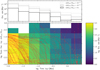 |
Fig. 11 Global rate of disc-truncating encounters for discs around stars with mass m* > 0.08 M⊙ throughout the evolution of our dynamical model. The top panel shows the rate of all truncating encounters that decrease the disc radius by at least 0.1 percent (light grey), 1 percent (grey) and 10 percent (black) of the pre-encounter radius. The colour scale of the bottom panel shows the encounter rates binned into both the time of the encounter (x-axis) and the degree of truncation (y-axis). Each logged encounter is shown by a pink square, and subsequent encounters for the same disc (if any) are connected by faint red lines. |
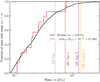 |
Fig. 12 Cumulative distribution function for the masses m* of stars with m* > 0.08 M⊙ in our simulation (black line), compared with those that underwent a truncating encounter −∆Rout/Rout > 0.01 (red line). The distributions are not significantly different, with KS test probability pKS = 0.87. We also show mass estimates for the stars with discs that are responsible for the observed external structure. We do not show uncertainties in these estimates for clarity, but errors quoted are typically approximately ±0.3 M⊙. The distribution of masses of stars that have been inferred to have experienced recent truncating encounters are significantly different from those in our simulation, with pKS = 0.023. |
4.5 Mechanisms to increase late encounter rates
Given the apparently high probability that the observed sample of discs with external structure produced during a recent star-disc encounter is incomplete, we consider a number of possibilities that may enhance the frequency of encounters late-on during the dynamical evolution of Taurus.
4.5.1 (Viscous) re-expansion
For discs that experience multiple encounters that are either unbound or in long period binaries, viscous angular momentum transport (e.g. Lynden-Bell & Pringle 1974) or infall of material from the ISM (e.g. Padoan et al. 2005; Manara et al. 2018; Kuffmeier et al. 2023; Gupta et al. 2023; Padoan et al. 2024; Winter et al. 2024) may replenish outer disc material such that subsequent encounters will have a stronger influence than under our assumption that disc radius is fixed. This replenishment should be correlated with stellar mass (as suggested by observed stellar accretion rates – Manara et al. 2017), so this would also preferentially enhance truncating encounter rates for high mass stars, consistent with observations (Section 4.4). Conversely, if angular momentum is extracted by magnetohydrodynamic winds (e.g. Bai & Stone 2013) then this could exacerbate the encounter rate problem.
4.5.2 Self-gravity of the interstellar medium
As discussed in Section 3.12, for practical reasons we have ignored ISM self-gravity in our calculations. If included, we would expect this self-gravity to increase the time for which groups of stars remain bound and therefore potentially enhance the frequency of truncating encounters at late times. This in-of-itself may explain any shortcoming in the frequency of encounters in our model compared to observations. However, for this to keep stars bound together, gas must be at approximately the critical density to undergo gravitational collapse. On length scales λ relevant for the Taurus region (συ ≫ Cs and λ ≪ h, the galactic scale height), this is effectively the Jeans criterion: the gravitational potential must balance the turbulent energy. At such densities, as discussed above, a number of authors have suggested that disc replenishment by Bondi-Hoyle-Lyttleton (BHL) accretion may be substantial (Padoan et al. 2005; Throop & Bally 2008; Kuffmeier et al. 2023; Winter et al. 2024).
To test whether we expect stellar dynamics-altering ISM self-gravity to also substantially replenish protoplanetary discs, we derived the critical density ρc as a function of λ following Winter et al. (2024), shown as the black line in Figure 13. We then estimated the expected typical BHL accretion rate:
 (14)
(14)
for a solar mass star m*= 1 M⊙, shown as the red dashed line in Figure 13. Here συ ∝ λ0.5 as we assumed when implementing kinematic substructure. For typical regions of size λ ~ 1 pc (Schmalzl et al. 2010; Joncour et al. 2018), our calculations imply a BHL accretion rate ṀBHL ~ 10−8 M⊙ yr−1, comparable to observed stellar accretion rates (e.g. Manara et al. 2023). Therefore, if local dynamics is influenced by ISM self-gravity, we expect this also to replenish protoplanetary discs as discussed above in Section 4.5.1.
We summarise that, while we cannot rule out ISM self-gravity as a possible driver of present day encounters in Taurus, this would have extremely interesting consequences for disc evolution. In particular, it would imply that replenishment from the ISM is indeed common.
 |
Fig. 13 Critical density at which the ISM is bound against turbulent pressure (black line, left-hand-side y-axis) and the resultant Bondi-Hoyle-Lyttleto (BHL) accretion rate for a solar mass star (red dashed line, right-hand-side y-axis). Both are shown as a function of spatial scale λ. |
4.5.3 Tidal torques from the disc on the perturber
If the disc is sufficiently massive and the encounter sufficiently close, then it is possible that the tidal dissipation of the orbital energy of the perturber leads to capture and tightening of the bound orbit (Clarke & Pringle 1993; Ostriker 1994; Muñoz et al. 2015). In this case the subsequent encounters may be stronger as the periastron separation decreases. This is a promising way to generate delayed strong encounters in binary/multiple systems where multiple encounters have occurred, particularly given the evidence for several close passages in the RW Aurigae system (Rodriguez et al. 2018). Since the disc mass is a super-linear function of star mass (e.g. Ansdell et al. 2016), this mechanism could also be more effective for perturbations to discs around massive stars. A key question however, is whether discs retain sufficient mass to generate orbital decay to the present day; this may be the subject of future hydrodynamic simulations for RW Aurigae and UX Tau.
4.5.4 Embedded planets or brown dwarfs
If brown dwarfs or massive planets form and remain embedded in the protoplanetary discs, then it is possible that during the encounter they undergo large eccentricity perturbations (Heggie & Rasio 1996) or chaotic evolution, perhaps to be captured by the perturbing star (e.g. Fregeau et al. 2004). This would effectively be a late-stage enhancement of the binary fraction, which may be expected to enhance the encounter rate. As for the previous two mechanisms, massive planets appear to be more common around high mass stars (Johnson et al. 2010). While an interesting possibility in the context of spiral arms in discs, given the presence of a stellar-mass perturber in the cases of RW Aurigae and UX Tau this does not appear to be a convincing explanation.
4.5.5 Spatial variation of the binary fraction
In our simulations, we initiated binaries independently of their location. It is plausible that binary formation is more probable in regions of enhanced local density, where enhanced tides can in principle result in fragmentation into multiple systems (Horton et al. 2001). This would enhance the degree to which binaries typically interact with other stars, and may therefore lead to enhanced encounter rates. However, RW Aurigae at least does not appear to be located in a region of high stellar density (e.g. Pfalzner & Govind 2021).
4.5.6 Prospects
While the explanations discussed in this section are not yet necessary based on existing constraints, two future developments may change this conclusion. First, the quantity of mass in the extended structure surrounding RW Aurigae and UX Tau could be a substantial fraction of the disc mass (that may imply |ΔRout/Rout| ≫ 10−2). Second, any new discoveries of extended structure in Taurus originating from a star-disc encounter will considerably increase the required encounter rate to Γenc ~ 680 Myr−1, much greater than the rate for even weak encounters in our model Γenc ~ 200 Myr−1. Should an additional recent encounter be discovered, and given the arguments outlined above, possibly the most promising mechanism for enhancing the encounter rate is the (viscous) re-expansion or ISM replenishment of the disc. This hypothesis should be quantitatively investigated in the event of additional discoveries.
5 Conclusions
We have presented an N-body model for the Taurus star-forming region which is physically and empirically motivated. Our initial stellar population is generated probabilistically from a turbulent gaseous medium, via a zoom-in on a Gaussian field using the cosmology simulation tool GENETIC (Stopyra et al. 2020). We applied the inferred size-velocity relation in Taurus to generate an initial velocity dispersion, combined with an empirically motivated binary population. Without any additional tuning, this yields a dynamical model with excellent agreement to the observed structure in Taurus by the metrics of the pair separation distribution and separation-velocity correlation. This has allowed us, for the first time, to accurately assess the global frequency of encounters in the Taurus star-forming region.
In this way we have shown that, like the bull that is its namesake, stars in the Taurus star-forming region rarely settle for one close encounter. Instead, star-disc systems act as stellar matadors, often enduring several close approaches with a neighbouring star. The closest approach distances change stochastically over time as binaries are themselves perturbed by low velocity neighbours. High order multiples can also form and break up on timescales much shorter than the lifetime of Taurus. As a result, strong encounters at the present day can occur in one of four ways. The most common are: during the evolution of a chaotic multiple system; when an eccentric binary is perturbed; or as a result of a close approach in a very long period eccentric binary. Random encounters between single stars are rare, with close encounters in Taurus being mostly mediated through a binary companion. These categories can be blurred, and in some sense to distinguish between binary and unbound encounters is a false dichotomy. Since binaries and nearby low velocity stars influence each other, inferring accurate encounter rates requires that the spatial and kinematic structure of a region is quantitatively taken into account.
Overall, ~1/4 of discs are truncated below 30 au by dynamical encounters. However, the majority of these dynamical truncation events happen in the first few 0.1 Myr of the cluster evolution, over the course of a few binary periods. After this time, the role of encounters in sculpting the overall distribution of disc radii is largely finished in a low density star-forming region such as Taurus.
Nonetheless, individual strong encounters still occur over the region as a whole, and we consider whether the examples of HV and DO Tau (Howard et al. 2013; Winter et al. 2018a), RW Aurigae (Dai et al. 2015; Rodriguez et al. 2018) and UX Tau (Zapata et al. 2020; Ménard et al. 2020) should be observed in our model. We conclude that events resembling HV and DO Tau can occur at a rate of ~10 Myr−1 and therefore, given that it has remained observable for ~0.1 Myr, observing one such event at any given time is expected. If weak encounters that eject only ~0.1–1 percent of the disc mass are responsible for the external structure around RW Aurigae and UX Tau, then they are also expected given the encounter rate Γenc ~ 100–200 Myr−1 in our model. However, we highlight that the systems that have been inferred to have experienced recent truncating encounters do not appear to be consistent with random drawing from the mass function, while those in our model are. This hints that the known sample of discs that have recently experienced truncating encounters is incomplete: just one more observational example would be in strong tension with our model, implying additional physics.
We discussed a number of physical mechanisms that should be explored by future work that may yield enhancements in the rate of truncating encounters, such as the tightening of binaries due to star-disc interaction (e.g. Muñoz et al. 2015) or re-expansion/replenishment in the outer regions of protoplanetary discs. We also show that substantial replenishment via BHL accretion must be proceeding if ISM self-gravity, which we neglect in this work, is significant for the dynamical evolution of high order multiples across the Taurus complex.
We summarise that star-disc encounters are an important probe of disc physics. This work highlights the need for a systematic search for extended structure generated by star-disc encounters in Taurus.
Acknowledgements
We thank the anonymous referees for their useful comments that helped improve the clarity of this paper. This project has received funding from the European Research Council (ERC) under the European Union’s Horizon research and innovation programme (grant agreement No. 101002188, project PROTOPLANETS, and grant agreement No. 101042275, project Stellar-MADE). A.J.W. has received funding from the European Union’s Horizon 2020 research and innovation programme under the Marie Skłodowska-Curie grant agreement No 101104656. L.S. was supported by NSFC grant Nos. 11890692, 12133008, and 12221003. L.S. thanks T Fang for support and acknowledges science research grants from NSFC, grant Nos. 11890692, 12133008, and 12221003. This work has made use of data from the European Space Agency (ESA) mission Gaia (https://www.cosmos.esa.int/gaia), processed by the Gaia Data Processing and Analysis Consortium (DPAC, https://www.cosmos.esa.int/web/gaia/dpac/consortium). Funding for the DPAC has been provided by national institutions, in particular the institutions participating in the Gaia Multilateral Agreement.
Appendix A Output frequency exploration
Our approach to computing the encounter frequency has been to post-process high frequency outputs, following the method described in Section 3.10. For our fiducial model, we adopt an output frequency of one every 323 years. While this frequency is sufficient to capture even binary encounters if the semi-major axis a ≳ 50 au, it is possible that in some instances binary-single or binary-binary interactions result in miscalculation of the true encounter properties. Here we test if such events may change our results.
While it would be laborious (and challenging) to check every single star’s encounter history in our sample for examples where our approach does not capture close encounters, we can more directly test our choice on the disc truncation history. We therefore decrease the output time step by factor ten (one every 32 years), and repeat the same analysis on the rate of disc truncation as before. The results are summarised in Figure A.1, which can be compared directly to Figure 11. Statistically and qualitatively, our results are very similar. We therefore conclude that our approach for extracting encounters is not substantially altering our conclusions. However, we do notice some small differences in the encounter history that correspond to a small number of individual encounter histories. These differences are not important for our conclusions, but we investigate them as follows.
We first identify an example of a system for which we observe differences in the encounter history depending on the output frequency. We show one such encounter history in Figure A.2 for our fiducial model, which is a chaotic triple interaction. The close encounters identified by our algorithm are shown as crosses. Comparison with the high frequency output simulation (Figure A.3) shows that at early times, both encounter histories are identical. They diverge after ~ 0.3 Myr, from which point the dynamics of the systems evolve chaotically to different end-states. This suggests that the differences in the encounter histories inferred from Figure A.1 compared to Figure 11 are not due to differences in our encounter-extraction algorithm, but differences in the N-body integration itself. While in principle changing the frequency of outputs should not alter the integration, NBODY6++ performs a number of accountancy operations at the time of output. It is possible that these operations slightly alter other numbers in the code that enter into numerical calculations via, for example, the adjustment of parameters. We demonstrate that altering the parameter adjustment time step (DTADJ) can have a similar influence on the dynamical evolution of chaotic multiples in Figure A.4, where we reduce this time step by five compared to our fiducial model.
We do not here investigate what changes to the output time step lead to an altered chaotic evolution of high order multiples when using the NBODY6++ code. By the nature of chaotic interactions, such changes may be tiny (such as machine precision) and in this case no particular solution is obviously more accurate. This is particularly irrelevant physically, since for these cases other processes may also change the dynamical outcome. However, we are satisfied that the statistical distribution of star-disc encounters our model is not dependent on our choice of output time step, and that our algorithm for extracting encounters is adequate for our purposes.
Appendix B Stochastic encounter history
To ensure that we are not dominated in our quantitative conclusions by stochastic variations in the encounter rates, we perform two additional numerical integrations of a Taurus-like region. We do this by performing two resampling experiments for the same density field as we adopt for our fiducial model, then adding a new binary population. The outcome comparing the encounter rates across all the simulations is shown in Figure B.1. Figures comparable to Figure 11 are shown in Figures B.2 and B.3. While we are not able to repeat the experiment enough times to gain a full distribution at each time interval, we can estimate a factor ~ 2 variation in the encounter rates is typical. We conclude that the rate of truncating encounters that we predict is only stochastic to within a factor of order unity.
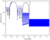 |
Fig. A.2 Example of a chaotic multiple interaction in our fiducial model. We show the separation of two neighbouring stars from a third star as a function of time. Crosses mark the location where the closest encounter is recorded by our post-processing analysis. |
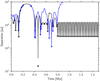 |
Fig. A.3 As in Figure A.2, but for the same stars but with a factor ten higher output frequency. |
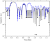 |
Fig. A.4 As in Figure A.2, but with a factor five smaller time step between the adjustment of simulation paramaters (DTADJ parameter in NBODY6 ++). |
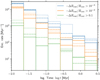 |
Fig. B.1 Stochastic variation of the encounter rate between different simulations (shown by different line styles). The colour of the lines refers to the threshold truncation used to define the encounter (as in Figure 11). |
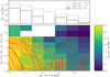 |
Fig. B.3 As in Figure B.2 but for a third random drawing of the stellar and binary population. |
References
- Aarseth, S. J. 2003, Gravitational N-Body Simulations (Cambridge: Cambridge University Press) [Google Scholar]
- Abt, H. A. 2006, ApJ, 651, 1151 [NASA ADS] [CrossRef] [Google Scholar]
- Adams, F. C., Proszkow, E. M., Fatuzzo, M., & Myers, P. C. 2006, ApJ, 641, 504 [NASA ADS] [CrossRef] [Google Scholar]
- Alaguero, A., Cuello, N., Ménard, F., et al. 2024, A&A, 687, A311 [NASA ADS] [CrossRef] [EDP Sciences] [Google Scholar]
- Andrews, S. M. 2020, ARA&A, 58, 483 [Google Scholar]
- Ansdell, M., Williams, J. P., van der Marel, N., et al. 2016, ApJ, 828, 46 [Google Scholar]
- Artymowicz, P., & Lubow, S. H. 1994, ApJ, 421, 651 [Google Scholar]
- Babusiaux, C., Fabricius, C., Khanna, S., et al. 2023, A&A, 674, A32 [NASA ADS] [CrossRef] [EDP Sciences] [Google Scholar]
- Baehr, H., & Zhu, Z. 2021, ApJ, 909, 135 [NASA ADS] [CrossRef] [Google Scholar]
- Bai, X.-N., & Stone, J. M. 2013, ApJ, 769, 76 [Google Scholar]
- Bastian, N., Lamers, H. J. G. L. M., de Mink, S. E., et al. 2013, MNRAS, 436, 2398 [CrossRef] [Google Scholar]
- Bate, M. R. 2018, MNRAS, 475, 5618 [Google Scholar]
- Beckwith, S. V. W., Sargent, A. I., Chini, R. S., & Guesten, R. 1990, AJ, 99, 924 [Google Scholar]
- Brunt, C. M. 2010, A&A, 513, A67 [NASA ADS] [CrossRef] [EDP Sciences] [Google Scholar]
- Burgers, J. 1948, in Advances in Applied Mechanics, A Mathematical Model Illustrating the Theory of Turbulence, eds. R. Von Mises, & T. Von Kármán (Amsterdam: Elsevier), 1, 171 [Google Scholar]
- Cabrit, S., Pety, J., Pesenti, N., & Dougados, C. 2006, A&A, 452, 897 [CrossRef] [EDP Sciences] [Google Scholar]
- Cadiou, C., Pontzen, A., Peiris, H. V., & Lucie-Smith, L. 2021, MNRAS, 508, 1189 [NASA ADS] [CrossRef] [Google Scholar]
- Clarke, C. J., & Pringle, J. E. 1993, MNRAS, 261, 190 [Google Scholar]
- Clarke, C. J., Gendrin, A., & Sotomayor, M. 2001, MNRAS, 328, 485 [NASA ADS] [CrossRef] [Google Scholar]
- Craig, J., & Krumholz, M. R. 2013, ApJ, 769, 150 [NASA ADS] [CrossRef] [Google Scholar]
- Cuello, N., Dipierro, G., Mentiplay, D., et al. 2019, MNRAS, 483, 4114 [Google Scholar]
- Cuello, N., Louvet, F., Mentiplay, D., et al. 2020, MNRAS, 491, 504 [Google Scholar]
- Cuello, N., Ménard, F., & Price, D. J. 2023, EPJ Plus, 138, 11 [NASA ADS] [Google Scholar]
- Dai, F., Facchini, S., Clarke, C. J., & Haworth, T. J. 2015, MNRAS, 449, 1996 [Google Scholar]
- De Rosa, R. J., & Kalas, P. 2019, AJ, 157, 125 [CrossRef] [Google Scholar]
- Dib, S., & Henning, T. 2019, A&A, 629, A135 [NASA ADS] [CrossRef] [EDP Sciences] [Google Scholar]
- Dong, R., Zhu, Z., Rafikov, R. R., & Stone, J. M. 2015, ApJ, 809, L5 [Google Scholar]
- Dong, R., Liu, H. B., Cuello, N., et al. 2022, Nat. Astron., 6, 331 [NASA ADS] [CrossRef] [Google Scholar]
- Douglas, T. A., Caselli, P., Ilee, J. D., et al. 2013, MNRAS, 433, 2064 [NASA ADS] [CrossRef] [Google Scholar]
- Duchêne, G., & Kraus, A. 2013, ARA&A, 51, 269 [Google Scholar]
- Duchêne, G., McCabe, C., Pinte, C., et al. 2010, ApJ, 712, 112 [CrossRef] [Google Scholar]
- Dullemond, C. P., Küffmeier, M., Goicovic, F., et al. 2019, A&A, 628, A20 [NASA ADS] [CrossRef] [EDP Sciences] [Google Scholar]
- El-Badry, K., Rix, H.-W., Tian, H., Duchêne, G., & Moe, M. 2019, MNRAS, 489, 5822 [NASA ADS] [CrossRef] [Google Scholar]
- Elmegreen, B. G., & Scalo, J. 2004, ARA&A, 42, 211 [Google Scholar]
- Esplin, T. L., & Luhman, K. L. 2019, AJ, 158, 54 [Google Scholar]
- Forgan, D., & Rice, K. 2010, MNRAS, 402, 1349 [CrossRef] [Google Scholar]
- Fregeau, J. M., Cheung, P., Portegies Zwart, S. F., & Rasio, F. A. 2004, MNRAS, 352, 1 [CrossRef] [Google Scholar]
- Gaia Collaboration (Prusti, T., et al.) 2016, A&A, 595, A1 [NASA ADS] [CrossRef] [EDP Sciences] [Google Scholar]
- Gaia Collaboration (Vallenari, A., et al.) 2023, A&A, 674, A1 [NASA ADS] [CrossRef] [EDP Sciences] [Google Scholar]
- Ghez, A. M., White, R. J., & Simon, M. 1997, ApJ, 490, 353 [NASA ADS] [CrossRef] [Google Scholar]
- Goldsmith, P. F., Heyer, M., Narayanan, G., et al. 2008, ApJ, 680, 428 [Google Scholar]
- Gupta, A., Miotello, A., Manara, C. F., et al. 2023, A&A, 670, L8 [NASA ADS] [CrossRef] [EDP Sciences] [Google Scholar]
- Ha, T., Li, Y., Kounkel, M., et al. 2022, ApJ, 934, 7 [NASA ADS] [CrossRef] [Google Scholar]
- Haisch, K. E., Jr., Lada, E. A., Piña, R. K., Telesco, C. M., & Lada, C. J. 2001, AJ, 121, 1512 [NASA ADS] [CrossRef] [Google Scholar]
- Hartigan, P., Edwards, S., & Ghandour, L. 1995, ApJ, 452, 736 [Google Scholar]
- Heggie, D. C., & Rasio, F. A. 1996, MNRAS, 282, 1064 [NASA ADS] [CrossRef] [Google Scholar]
- Heyer, M. H., & Brunt, C. M. 2004, ApJ, 615, L45 [NASA ADS] [CrossRef] [Google Scholar]
- Holmberg, J., Nordström, B., & Andersen, J. 2009, A&A, 501, 941 [NASA ADS] [CrossRef] [EDP Sciences] [Google Scholar]
- Horton, A. J., Bate, M. R., & Bonnell, I. A. 2001, MNRAS, 321, 585 [NASA ADS] [CrossRef] [Google Scholar]
- Howard, C. D., Sandell, G., Vacca, W. D., et al. 2013, ApJ, 776, 21 [Google Scholar]
- Johnson, J. A., Aller, K. M., Howard, A. W., & Crepp, J. R. 2010, PASP, 122, 905 [Google Scholar]
- Joncour, I., Duchêne, G., & Moraux, E. 2017, A&A, 599, A14 [NASA ADS] [CrossRef] [EDP Sciences] [Google Scholar]
- Joncour, I., Duchêne, G., Moraux, E., & Motte, F. 2018, A&A, 620, A27 [NASA ADS] [CrossRef] [EDP Sciences] [Google Scholar]
- Kraus, A. L., & Hillenbrand, L. A. 2009, ApJ, 704, 531 [Google Scholar]
- Kroupa, P. 2001, MNRAS, 322, 231 [NASA ADS] [CrossRef] [Google Scholar]
- Krumholz, M. R., McKee, C. F., & Bland-Hawthorn, J. 2019, ARA&A, 57, 227 [NASA ADS] [CrossRef] [Google Scholar]
- Kuffmeier, M., Goicovic, F. G., & Dullemond, C. P. 2020, A&A, 633, A3 [NASA ADS] [CrossRef] [EDP Sciences] [Google Scholar]
- Kuffmeier, M., Dullemond, C. P., Reissl, S., & Goicovic, F. G. 2021, A&A, 656, A161 [NASA ADS] [CrossRef] [EDP Sciences] [Google Scholar]
- Kuffmeier, M., Jensen, S. S., & Haugbølle, T. 2023, EPJ Plus, 138, 272 [NASA ADS] [Google Scholar]
- Lada, C. J., & Lada, E. A. 2003, ARA&A, 41, 57 [Google Scholar]
- Larson, R. B. 1981, MNRAS, 194, 809 [Google Scholar]
- Lépine, S., & Bongiorno, B. 2007, AJ, 133, 889 [Google Scholar]
- Li, D., Mustill, A. J., Davies, M. B., & Gong, Y.-X. 2024, MNRAS, 527, 386 [Google Scholar]
- Lichtenberg, T., Parker, R. J., & Meyer, M. R. 2016, MNRAS, 462, 3979 [NASA ADS] [CrossRef] [Google Scholar]
- Luhman, K. L. 2004, ApJ, 617, 1216 [Google Scholar]
- Luhman, K. L. 2023, AJ, 165, 37 [NASA ADS] [CrossRef] [Google Scholar]
- Lynden-Bell, D., & Pringle, J. E. 1974, MNRAS, 168, 603 [Google Scholar]
- Manara, C. F., Testi, L., Herczeg, G. J., et al. 2017, A&A, 604, A127 [NASA ADS] [CrossRef] [EDP Sciences] [Google Scholar]
- Manara, C. F., Morbidelli, A., & Guillot, T. 2018, A&A, 618, L3 [NASA ADS] [CrossRef] [EDP Sciences] [Google Scholar]
- Manara, C. F., Tazzari, M., Long, F., et al. 2019, A&A, 628, A95 [NASA ADS] [CrossRef] [EDP Sciences] [Google Scholar]
- Manara, C. F., Ansdell, M., Rosotti, G. P., et al. 2023, ASP Conf. Ser., 534, 539 [NASA ADS] [Google Scholar]
- Ménard, F., Cuello, N., Ginski, C., et al. 2020, A&A, 639, L1 [EDP Sciences] [Google Scholar]
- Meru, F., Juhász, A., Ilee, J. D., et al. 2017, ApJ, 839, L24 [Google Scholar]
- Miotello, A., Kamp, I., Birnstiel, T., Cleeves, L. C., & Kataoka, A. 2023, ASP Conf. Ser., 534, 501 [NASA ADS] [Google Scholar]
- Moe, M., & Di Stefano, R. 2017, ApJS, 230, 15 [Google Scholar]
- Moeckel, N., & Bate, M. R. 2010, MNRAS, 404, 721 [NASA ADS] [CrossRef] [Google Scholar]
- Muñoz, D. J., Kratter, K., Vogelsberger, M., Hernquist, L., & Springel, V. 2015, MNRAS, 446, 2010 [CrossRef] [Google Scholar]
- Münch, G. 1958, Rev. Mod. Phys., 30, 1035 [CrossRef] [Google Scholar]
- Niu, Z., Yuan, H., Wang, S., & Liu, J. 2021, ApJ, 922, 211 [NASA ADS] [CrossRef] [Google Scholar]
- Nordlund, Å. K., & Padoan, P. 1999, in Interstellar Turbulence, eds. J. Franco, & A. Carraminana (Cambridge: Cambridge University Press), 218 [CrossRef] [Google Scholar]
- Ostriker, E. C. 1994, ApJ, 424, 292 [NASA ADS] [CrossRef] [Google Scholar]
- Ostriker, E. C., Gammie, C. F., & Stone, J. M. 1999, ApJ, 513, 259 [NASA ADS] [CrossRef] [Google Scholar]
- Padoan, P., Jones, B. J. T., & Nordlund, Å. P. 1997, ApJ, 474, 730 [NASA ADS] [CrossRef] [Google Scholar]
- Padoan, P., Kritsuk, A., Norman, M. L., & Nordlund, Å. 2005, ApJ, 622, L61 [NASA ADS] [CrossRef] [Google Scholar]
- Padoan, P., Pan, L., Pelkonen, V.-M., Haugboelle, T., & Nordlund, A. 2024, arXiv e-prints [arXiv:2405.07334] [Google Scholar]
- Parker, R. J. 2023, MNRAS arXiv e-prints [arXiv:2308.05790] [Google Scholar]
- Parker, R. J., & Schoettler, C. 2023, ApJ, 952, L16 [NASA ADS] [CrossRef] [Google Scholar]
- Pearson, S. G., & McCaughrean, M. J. 2023, arXiv e-prints [arXiv:2310.01231] [Google Scholar]
- Pfalzner, S. 2008, A&A, 492, 735 [NASA ADS] [CrossRef] [EDP Sciences] [Google Scholar]
- Pfalzner, S., & Govind, A. 2021, ApJ, 921, 90 [NASA ADS] [CrossRef] [Google Scholar]
- Pfalzner, S., Vogel, P., Scharwächter, J., & Olczak, C. 2005, A&A, 437, 967 [CrossRef] [EDP Sciences] [Google Scholar]
- Plunkett, A. L., Fernández-López, M., Arce, H. G., et al. 2018, A&A, 615, A9 [NASA ADS] [CrossRef] [EDP Sciences] [Google Scholar]
- Portegies Zwart, S., & Hochart, E. 2023, arXiv e-prints [arXiv:2312.04645] [Google Scholar]
- Qian, L., Li, D., Gao, Y., Xu, H., & Pan, Z. 2018, ApJ, 864, 116 [CrossRef] [Google Scholar]
- Rasmussen, C. E., & Williams, C. K. 2006, Gaussian Processes for Machine Learning (Berlin: Springer), 1 [Google Scholar]
- Ren, B., Dong, R., van Holstein, R. G., et al. 2020, ApJ, 898, L38 [NASA ADS] [CrossRef] [Google Scholar]
- Rodriguez, J. E., Loomis, R., Cabrit, S., et al. 2018, ApJ, 859, 150 [Google Scholar]
- Rota, A. A., Manara, C. F., Miotello, A., et al. 2022, A&A, 662, A121 [NASA ADS] [CrossRef] [EDP Sciences] [Google Scholar]
- Schmalzl, M., Kainulainen, J., Quanz, S. P., et al. 2010, ApJ, 725, 1327 [NASA ADS] [CrossRef] [Google Scholar]
- Shara, M. M., Hurley, J. R., & Mardling, R. A. 2016, ApJ, 816, 59 [NASA ADS] [CrossRef] [Google Scholar]
- Shuai, L., Ren, B. B., Dong, R., et al. 2022, ApJS, 263, 31 [NASA ADS] [CrossRef] [Google Scholar]
- Spurzem, R. 1999, J. Comput. Appl. Math., 109, 407 [CrossRef] [Google Scholar]
- Spurzem, R., Giersz, M., Heggie, D. C., & Lin, D. N. C. 2009, ApJ, 697, 458 [Google Scholar]
- Stapelfeldt, K. R., Ménard, F., Watson, A. M., et al. 2003, ApJ, 589, 410 [NASA ADS] [CrossRef] [Google Scholar]
- Stopyra, S., Pontzen, A., Peiris, H., Roth, N., & Rey, M. 2020, Astrophysics Source Code Library [record ascl:2006.020] [Google Scholar]
- Stopyra, S., Pontzen, A., Peiris, H., Roth, N., & Rey, M. P. 2021, ApJS, 252, 28 [CrossRef] [Google Scholar]
- Tabone, B., Rosotti, G. P., Cridland, A. J., Armitage, P. J., & Lodato, G. 2022, MNRAS, 512, 2290 [NASA ADS] [CrossRef] [Google Scholar]
- Throop, H. B., & Bally, J. 2008, AJ, 135, 2380 [NASA ADS] [CrossRef] [Google Scholar]
- Vazquez-Semadeni, E. 1994, ApJ, 423, 681 [Google Scholar]
- Virtanen, P., Gommers, R., Oliphant, T. E., et al. 2020, Nat. Methods, 17, 261 [Google Scholar]
- Vorobyov, E. I., Steinrueck, M. E., Elbakyan, V., & Guedel, M. 2017, A&A, 608, A107 [NASA ADS] [CrossRef] [EDP Sciences] [Google Scholar]
- Vorobyov, E. I., Elbakyan, V. G., Liu, H. B., & Takami, M. 2021, A&A, 647, A44 [EDP Sciences] [Google Scholar]
- Wang, L., Spurzem, R., Aarseth, S., et al. 2015, MNRAS, 450, 4070 [NASA ADS] [CrossRef] [Google Scholar]
- Wang, Y., Perna, R., & Zhu, Z. 2024, Nat. Astron., 8, 756 [NASA ADS] [CrossRef] [Google Scholar]
- Winter, A. J., & Haworth, T. J. 2022, EPJ Plus, 137, 1132 [NASA ADS] [Google Scholar]
- Winter, A. J., Booth, R. A., & Clarke, C. J. 2018a, MNRAS, 479, 5522 [Google Scholar]
- Winter, A. J., Clarke, C. J., Rosotti, G., & Booth, R. A. 2018b, MNRAS, 475, 2314 [Google Scholar]
- Winter, A. J., Clarke, C. J., Rosotti, G., et al. 2018c, MNRAS, 478, 2700 [Google Scholar]
- Winter, A. J., Clarke, C. J., Rosotti, G., & Giersz, M. 2022, MNRAS, 515, 2837 [NASA ADS] [CrossRef] [Google Scholar]
- Winter, A. J., Benisty, M., & Andrews, S. M. 2024, ApJ, 972, L9 [NASA ADS] [CrossRef] [Google Scholar]
- Woitas, J., Leinert, C., & Köhler, R. 2001, A&A, 376, 982 [NASA ADS] [CrossRef] [EDP Sciences] [Google Scholar]
- Zapata, L. A., Rodríguez, L. F., Fernández-López, M., et al. 2020, ApJ, 896, 132 [Google Scholar]
- Zinnecker, H., McCaughrean, M. J., & Wilking, B. A. 1993, in Protostars and Planets III, eds. E. H. Levy, & J. I. Lunine (Tucson: University of Arizona Press), 429 [Google Scholar]
All Figures
|
Fig. 1 Proper motion difference as a function of angular separation on the plane of the sky for nearest neighbours in the Luhman (2023) sample for Taurus. Red data points are the observed sample, with uncertainties propagated from Gaia uncertainties. The black line shows the velocity dispersion as a function of separation we adopt for our model, with a Keplerian component that dominates at small separations. The transition between the two power-laws is the break between the binary and individual systems (~5 × 10⁴ au, comparable to the galactic tidal radius for typical stars). The colour bar shows the corresponding Maxwell-Boltzmann distribution, normalised for each separation. See text for details. |
| In the text | |
|
Fig. 2 Illustration of how we selected a box from which to generate a lognormal density field from a larger-scale, low resolution lognormal density field. We illustrate the underlying density grid by drawing faint black points with density proportional to the local density field. Cyan points indicate our selection of the top 20 density maxima from the density field. The red star indicates the position of the adopted box centre. The dashed red lines indicate the boundary of the new zoom-in box. |
| In the text | |
|
Fig. 3 Histogram showing the distribution of companions at a given semi-major axis (left) eccentricity (middle) and mass ratio (right) for primary stars with masses m* > 0.08 M⊙. The red histogram is for those pairs we define as ultrawide pairs, while the blue shows the binaries. |
| In the text | |
|
Fig. 4 Histogram of stellar masses in our dynamical model for Taurus. The solid black shows all stars including binary companions, while the red line is just the primaries and single stars. The black dashed line corresponds to the number that would be expected in each bin from the Kroupa (2001) IMF (Equation (5)). The bin sizes are similar to those adopted by Luhman (2004) in Figure 13, top panel. |
| In the text | |
|
Fig. 5 Proper motion difference versus angular separation assuming a distance of 140 pc for nearest neighbours from the initial conditions in our model. The black line shows the one dimensional velocity dispersion as a function of separation and the colour bar shows the normalised Maxwell-Boltzmann distribution for each separation, as in Figure 1. |
| In the text | |
|
Fig. 6 Normalised pair surface density |
| In the text | |
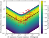 |
Fig. 7 As in Figure 5, except for our simulation after 1 Myr of evolution. |
| In the text | |
|
Fig. 8 One-point (Ψ, blue points) and two-point (ξ, grey points) correlation functions computed from our model at 1 Myr. The red line shows the Ψ ∝ ∆R−1.5 relationship for ∆R < 0.2° and the two dashed black lines enclose the region of inhibition (where Ψ < 1), as inferred by Joncour et al. (2017, see their Figure 4). |
| In the text | |
|
Fig. 9 Spatial distribution of stars (mass > 0.08 M⊙) at 1 Myr and contemporary disc-truncating encounters in our simulation. We show as coloured star or square symbols the location of all stars that underwent encounters yielding a fractional truncation −∆Rout/Rout > 0.01 over the age range 1 ± 0.2 Myr. Encounters that yielded −∆Rout/Rout > 0.1 are highlighted with red circles. In the panels along the top we show the separation between specific stars and their stellar neighbours over the first 1.5 Myr of the simulation. Each line represents the distance to a single stellar neighbour, linearly interpolated between snapshots, where neighbours that are one of the two closest stars at any given time step are included (if they pass within 104 au). In each plot, we mark the location of a logged ‘closest approach’ as a cross (inferred analytically from the closest time step – see Section 3.10). |
| In the text | |
|
Fig. 10 Disc outer radius Rout evolution for the population of stars with m* > 0.08 M⊙ in our simulation. The colour bar shows the time at which the distribution is measured. The initial outer radius distribution is shown in red. |
| In the text | |
|
Fig. 11 Global rate of disc-truncating encounters for discs around stars with mass m* > 0.08 M⊙ throughout the evolution of our dynamical model. The top panel shows the rate of all truncating encounters that decrease the disc radius by at least 0.1 percent (light grey), 1 percent (grey) and 10 percent (black) of the pre-encounter radius. The colour scale of the bottom panel shows the encounter rates binned into both the time of the encounter (x-axis) and the degree of truncation (y-axis). Each logged encounter is shown by a pink square, and subsequent encounters for the same disc (if any) are connected by faint red lines. |
| In the text | |
|
Fig. 12 Cumulative distribution function for the masses m* of stars with m* > 0.08 M⊙ in our simulation (black line), compared with those that underwent a truncating encounter −∆Rout/Rout > 0.01 (red line). The distributions are not significantly different, with KS test probability pKS = 0.87. We also show mass estimates for the stars with discs that are responsible for the observed external structure. We do not show uncertainties in these estimates for clarity, but errors quoted are typically approximately ±0.3 M⊙. The distribution of masses of stars that have been inferred to have experienced recent truncating encounters are significantly different from those in our simulation, with pKS = 0.023. |
| In the text | |
|
Fig. 13 Critical density at which the ISM is bound against turbulent pressure (black line, left-hand-side y-axis) and the resultant Bondi-Hoyle-Lyttleto (BHL) accretion rate for a solar mass star (red dashed line, right-hand-side y-axis). Both are shown as a function of spatial scale λ. |
| In the text | |
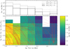 |
Fig. A.1 As in Figure 11, but for a factor ten higher output frequency. |
| In the text | |
|
Fig. A.2 Example of a chaotic multiple interaction in our fiducial model. We show the separation of two neighbouring stars from a third star as a function of time. Crosses mark the location where the closest encounter is recorded by our post-processing analysis. |
| In the text | |
|
Fig. A.3 As in Figure A.2, but for the same stars but with a factor ten higher output frequency. |
| In the text | |
|
Fig. A.4 As in Figure A.2, but with a factor five smaller time step between the adjustment of simulation paramaters (DTADJ parameter in NBODY6 ++). |
| In the text | |
|
Fig. B.1 Stochastic variation of the encounter rate between different simulations (shown by different line styles). The colour of the lines refers to the threshold truncation used to define the encounter (as in Figure 11). |
| In the text | |
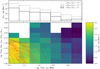 |
Fig. B.2 As in Figure 11 but for a second random drawing of the stellar and binary population. |
| In the text | |
|
Fig. B.3 As in Figure B.2 but for a third random drawing of the stellar and binary population. |
| In the text | |
Current usage metrics show cumulative count of Article Views (full-text article views including HTML views, PDF and ePub downloads, according to the available data) and Abstracts Views on Vision4Press platform.
Data correspond to usage on the plateform after 2015. The current usage metrics is available 48-96 hours after online publication and is updated daily on week days.
Initial download of the metrics may take a while.