A Virgo Environmental Survey Tracing Ionised Gas Emission (VESTIGE)

C. R. Morgan; M. L. Balogh; A. Boselli; M. Fossati; C. Lawlor-Forsyth; E. Sazonova; P. Amram; M. Boquien; J. Braine; L. Cortese; P. Côté; J. C. Cuillandre; L. Ferrarese; S. Gwyn; G. Hensler; Junais Junais; J. Roediger

doi:10.1051/0004-6361/202449225

Home

All issues

Volume 691 (November 2024)

A&A, 691 (2024) A20

Full HTML

Open Access

Issue		A&A Volume 691, November 2024


Article Number		A20
Number of page(s)		22
Section		Extragalactic astronomy
DOI		https://doi.org/10.1051/0004-6361/202449225
Published online		28 October 2024

A&A, 691, A20 (2024)

XVI. The ubiquity of truncated star-forming discs across the Virgo cluster environment

C. R. Morgan¹^,2^⋆, M. L. Balogh¹^,2, A. Boselli³^,4, M. Fossati⁵^,6, C. Lawlor-Forsyth¹^,2, E. Sazonova¹^,2, P. Amram³, M. Boquien⁷, J. Braine⁸, L. Cortese⁹^,10, P. Côté¹¹, J. C. Cuillandre¹², L. Ferrarese¹¹, S. Gwyn¹¹, G. Hensler¹³, Junais¹⁴ and J. Roediger¹¹

¹ Waterloo Centre for Astrophysics, University of Waterloo, Waterloo, ON N2L 3G1, Canada
² Department of Physics and Astronomy, University of Waterloo, Waterloo, ON N2L 3G1, Canada
³ Aix-Marseille Univ., CNRS, CNES, LAM, Marseille, France
⁴ INAF – Osservatorio Astronomico di Cagliari, Via della Scienza 5, 09047 Selargius, Italy
⁵ Universitá di Milano-Bicocca, Piazza della Scienza 3, 20100 Milano, Italy
⁶ INAF – Osservatorio Astronomico di Brera, Via Brera 28, 21021 Milano, Italy
⁷ Université Côte d’Azur, Observatoire de la Côte d’Azur, CNRS, Laboratoire Lagrange, 06000 Nice, France
⁸ Laboratoire d’Astrophysique de Bordeaux, Univ. Bordeaux, CNRS, B18N, Allée Geoffroy Saint-Hilaire, 33615 Pessac, France
⁹ International Centre for Radio Astronomy Research (ICRAR), University of Western Australia, Crawley, WA 6009, Australia
¹⁰ Australian Research Council, Centre of Excellence for All Sky Astrophysics in 3 Dimensions (ASTRO 3D), Australia
¹¹ National Research Council of Canada, Herzberg Astronomy and Astrophysics Research Centre, Victoria, BC V9E 2E7, Canada
¹² AIM, CEA, CNRS, Université Paris-Saclay, Université de Paris, 91191 Gif-sur-Yvette, France
¹³ Department of Astrophysics, University of Vienna, Türkenschanzstrasse 17, 1180 Vienna, Austria
¹⁴ National Centre for Nuclear Research, Pasteura 7, 02-093 Warsaw, Poland

^⋆ Corresponding author; crmorgan@uwaterloo.ca

Received: 12 January 2024
Accepted: 11 September 2024

Abstract

We examine the prevalence of truncated star-forming discs in the Virgo cluster down to M_* ≃ 10⁷ M_⊙. This work makes use of deep, high-resolution imaging in the Hα+[N II] narrow-band from the Virgo Environmental Survey Tracing Ionised Gas Emission (VESTIGE) and optical imaging from the Next Generation Virgo Survey (NGVS). To aid in the understanding of the effects of the cluster environment on star formation in Virgo galaxies, we take a physically motivated approach to define the edge of the star-forming disc via a drop-off in the radial specific star formation rate profile. A comparison with the expected sizes of normal galactic discs provides a measure of how truncated star-forming discs are in the cluster. We find that truncated star-forming discs are nearly ubiquitous across all regions of the Virgo cluster, including beyond the virial radius (0.974 Mpc). The majority of truncated discs at large cluster-centric radii are of galaxies likely on their first infall. As the intra-cluster medium density is low in this region, it is difficult to explain this population with solely ram-pressure stripping. A plausible explanation is that these galaxies are undergoing starvation of their gas supply before ram-pressure stripping becomes the dominant quenching mechanism. A simple model of starvation shows that this mechanism can produce moderate disc truncations within 1−2 Gyr. This model is consistent with ‘slow-then-rapid’ or ‘delayed-then-rapid’ quenching, whereby the early starvation mode drives disc truncations without significant change to the integrated star formation rate, and the later ram-pressure stripping mode rapidly quenches the galaxy. The origin of starvation may be in the group structures that exist around the main Virgo cluster, which indicates the importance of understanding pre-processing of galaxies beyond the cluster virial radius.

Key words: galaxies: evolution / galaxies: fundamental parameters / galaxies: clusters: individual: Virgo / galaxies: star formation

© The Authors 2024

Open Access article, published by EDP Sciences, under the terms of the Creative Commons Attribution License (https://creativecommons.org/licenses/by/4.0), which permits unrestricted use, distribution, and reproduction in any medium, provided the original work is properly cited.

This article is published in open access under the Subscribe to Open model. Subscribe to A&A to support open access publication.

1. Introduction

Galaxies in the local Universe exhibit a bimodality in terms of their colour and star formation rate (SFR). Star-forming (SF) galaxies are blue in colour and are dominated by a disc shape and features such as spiral arms where ongoing star formation occurs. Conversely, ‘quiescent’ galaxies are typically ellipsoidal and red in colour, containing evolved stellar populations with little ongoing star formation. Measurements of the redshift evolution of the stellar mass function (SMF) have shown that the population of quiescent galaxies has built up over time, indicating that galaxies transition or ‘quench’ from actively SF to quiescent (e.g. Faber et al. 2007). Galaxy quenching is known to be a function of mass, as the quiescent fraction is greater at the high end of the SMF in all environments and at all redshifts (Peng et al. 2010; Muzzin et al. 2013; Lin et al. 2014; Balogh et al. 2016).

Galaxies are also known to evolve as a function of their environment (Oemler 1974; Dressler 1980; Butcher & Oemler 1984). Galaxies in clusters, particularly those at low redshift, exhibit lower rates of star formation (Balogh et al. 1997, 1998; Lewis et al. 2002; Gómez et al. 2003; Kauffmann et al. 2004; Baldry et al. 2006; Weinmann et al. 2006; Wetzel et al. 2012; Gavazzi et al. 2013a; Boselli et al. 2023a) and are more gas-deficient (Giovanelli & Haynes 1985; Cayatte et al. 1990; Gavazzi et al. 2005; Cortese et al. 2011; Boselli et al. 2014a; Alberts et al. 2022) than galaxies in the field. The observed morphology of galaxies also varies by environment, with the fraction of quiescent elliptical galaxies increasing as a function of density (Dressler 1980; Huchra et al. 1983; Goto et al. 2003). Measurements of this morphology-density relation (e.g. Dressler et al. 1997; Sazonova et al. 2020) and the SFR-density relation (e.g. Quadri et al. 2012; Cooke et al. 2016; Kawinwanichakij et al. 2017; Strazzullo et al. 2019; van der Burg et al. 2020) up to z ∼ 2 indicate that the drivers of environmental quenching in clusters were in place at earlier epochs.

A variety of different environmentally driven mechanisms are known to quench galaxies in clusters (e.g. Boselli & Gavazzi 2006, 2014). Galaxies can interact with each other through direct mergers, which can induce starbursts in the resulting system, alter the morphology of the merged galaxy, and drive active galactic nucleus (AGN) feedback (Barnes 2004; Saitoh et al. 2009; Rich et al. 2011; Kelkar et al. 2020; Lotz et al. 2021). Close encounters can strip material to form tidal arms, and can cause gas to lose angular momentum and fall to the centre of the galaxy where a nuclear starburst is induced (‘harassment’; Moore et al. 1996, 1998). Galaxies falling into clusters will also interact with the hot intra-cluster medium (ICM), during which ram-pressure stripping (RPS) serves to actively strip gas from the disc of the galaxy, removing the fuel necessary for sustained star formation (Gunn & Gott 1972; Boselli et al. 2022). Additionally, infalling galaxies can undergo ‘starvation’ or ‘strangulation’ as the potential of the galactic dark matter halo becomes subdominant to the cluster potential, preventing the accretion of fresh gas (Larson et al. 1980). The existing hot gas contained within the subhalo of the galaxy may also be stripped off via ram-pressure and/or tidal forces (Balogh et al. 2000; McCarthy et al. 2008; Kawata & Mulchaey 2008; Bekki 2009), or prevented from cooling due to feedback. Starved galaxies passively quench as they exhaust their remaining cold gas supply.

Each quenching mechanism produces signatures that can be observed and measured to find trends with mass and environment. For example, RPS can produce elaborate tails of stripped gas that extend beyond the optical disc (e.g. Gavazzi et al. 2001; Kenney et al. 2004; Chung et al. 2007). In some cases, star formation can occur in the stripped material, producing stars in the tails that can result in a ‘jellyfish’ appearance in the optical (e.g. Smith et al. 2010; Ebeling et al. 2014; Poggianti et al. 2016). Over time, RPS will lead to a truncated SF disc as all the gas is stripped from the outside in (see Boselli et al. 2022 for a comprehensive review on the effects of RPS).

In many cases, multiple mechanisms could be quenching galaxies at the same time, or in sequence (e.g. Cortese et al. 2021). Understanding the interplay of various mechanisms in the overall evolutionary picture is an area of ongoing research. For example, while the morphological signatures of RPS may be present in many galaxies, that does not necessarily imply that RPS has been solely responsible for reducing the gas content of the galaxy. A galaxy that has been pre-processed may become even more susceptible to RPS if its gas has been initially displaced by tidal interactions (e.g. Serra et al. 2023) or its gas content has been reduced by starvation.

Hα emission is a powerful tool with which to observe morphological signatures of environmental quenching mechanisms, since it traces star formation on 10 Myr timescales (e.g. Kennicutt 1998). Early studies such as Moss & Whittle (1993, 2000) undertook Hα surveys of local rich clusters, observing concentrated Hα emission that suggested induced star formation due to tidal interactions, particularly for galaxies in denser environments. Gavazzi et al. (2006, 2013b) showed that Hα emission is correlated with H I gas content in galaxies, and that the specific star formation rate (sSFR) is correlated with Hubble type morphology. Koopmann & Kenney (2004) and Fossati et al. (2013) compared the sizes of SF discs measured in Hα with optical bands to show truncations in the Virgo cluster. More recently, integral field unit (IFU) spectroscopy has become a powerful tool for observing Hα emission on a spatially resolved scale across the planes of galaxies. The GASP survey (Gas Stripping Phenomena in galaxies with MUSE; Poggianti et al. 2017) is a programme that has targeted more than 100 nearby jellyfish galaxy candidates to study the kinematics and physical properties of the ionised gas being stripped from the galactic discs. With the advent of IFU spectroscopy and deep, high-resolution imaging with surveys like VESTIGE (the Virgo Environmental Survey Tracing Ionised Gas Emission; Boselli et al. 2018a), detailed Hα maps can now be observed for nearby galaxies, allowing star formation and quenching mechanisms to be studied on a spatially resolved scale.

The Virgo cluster is of particular interest to the study of environmentally driven quenching mechanisms due in part to its proximity. At a distance of 16.5 Mpc (Mei et al. 2007), Virgo is the closest massive galaxy cluster, and has been imaged on sub-kiloparsec scales with many recent surveys, including in the UV (GUViCS; Boselli et al. 2011), optical (NGVS; Ferrarese et al. 2012), and Hα (VESTIGE; Boselli et al. 2018a). Indeed, RPS has been identified as a likely driver of environmental quenching in Virgo through many studies of individual objects and small samples of galaxies (Koopmann & Kenney 2004; Koopmann et al. 2006; Cortese et al. 2012; Fossati et al. 2013; Chung et al. 2009; Boselli et al. 2016; Junais et al. 2022; see Boselli et al. 2022 for a review). These studies have identified tails of stripped gas and truncated discs associated with RPS. The majority of SF galaxies in Virgo are also known to be H I-deficient (Chamaraux et al. 1980; Giovanelli & Haynes 1983; Gavazzi et al. 2005; Boselli et al. 2023a) with truncated gas discs (Cayatte et al. 1990, 1994; Chung et al. 2009; Boselli et al. 2014a; Zabel et al. 2022), indicating the presence of mechanisms to either remove gas or prevent a fresh supply of hot gas from cooling onto galactic discs.

Measuring the size of the SF disc (for example with UV, Hα, or 24 μm imaging) provides information on the radial extent of star formation, and can be compared to the disc size measured in optical bands to allow a measurement of disc truncation. This is a common method in the literature to determine the presence of an outside in quenching mechanism (e.g. Koopmann & Kenney 2004; Cortese et al. 2012; Fossati et al. 2013; Finn et al. 2018). A popular measurement of the size of the galactic disc is the effective radius, or half-light radius¹. The total light of the galaxy can be measured through extrapolation of the flux growth curve, or by using a low-surface brightness isophote. However, the effective radius is sensitive to the concentration of light in the galaxy; this value may be different between the SF and optical discs (e.g. Trujillo et al. 2020; Chamba et al. 2020). Taking the ratio of isophotal radii in SF and optical bands is another method to quantify truncation (e.g. Cortese et al. 2012), where the isophotal radii provide a more meaningful representation of the extent of the disc. In using a Sérsic fit to define the radial profile of a galaxy, the effective or isophotal radius are well-defined measures of size, but neither correspond to an actual edge of the disc.

Chamba et al. (2022, hereafter C22) identified the edges of galaxies (R_edge) based on visual identification of turn-off points in their stellar mass surface density and optical colour profiles. They showed that this visually identified edge corresponds to a critical stellar mass surface density that depends weakly on the integrated stellar mass of the galaxy. For massive disc galaxies (M_* ≳ 10⁹ M_⊙), this turn-off corresponds with the edge of the SF disc, as is indicated by a sudden change in the slope of the UV surface brightness profiles. As such, the edge of the stellar disc should correspond with the edge of the SF disc for normal, SF galaxies. A follow-up work, (Chamba et al. 2024) found that galaxies in the Fornax cluster have edges that occur at higher stellar mass surface density, giving rise to smaller measured disc sizes.

In addition to physical disc edges, various studies have observed other features that represent deviations from a single exponential fit to a surface brightness profile. Since the work of Freeman (1970), it has been shown that galaxy discs are often best fit by two exponential components, separated by a break, where the outer part of the disc may have a steeper (Type II) or shallower (Type III) slope than the inner part (e.g. Pohlen & Trujillo 2006; Hunter & Elmegreen 2006; Erwin et al. 2008; Herrmann et al. 2013, 2016; Watkins et al. 2019). These breaks are often identified in optical bands, though comparisons with SF bands (UV and Hα) show that in some cases, the breaks are more even more significant in these bands than in the optical (e.g. Herrmann et al. 2016), suggesting that these breaks may correspond to the edge of the SF disc.

In this work we look to quantify, in the Virgo cluster, the presence of galactic discs with a truncated SF component relative to the underlying optical disc. Boselli et al. (2020) identified truncated SF discs in a subset of VESTIGE galaxies through the decline in the number density of H II regions. Other previous studies of truncated SF discs in Virgo were limited to massive galaxies (e.g. Koopmann & Kenney 2004; Boselli et al. 2022) or used size measurements such as the effective radius that do not explicitly trace the edge of the SF disc (e.g. Fossati et al. 2013). In our approach, we take advantage of the unique NGVS and VESTIGE data to analyse sSFR profiles and identify a physically meaningful edge to the SF disc. By comparing the edge of the SF disc to the expected disc size based on a comparable field sample, we can quantify how truncated the SF discs are in the Virgo cluster. With our cluster-wide sample that includes all SF galaxies within the cluster virial radius and a sample beyond, we look to provide insights into the different possible quenching pathways that may produce the observed distribution of truncated discs.

A description of the data used in this work is outlined in Section 2. In Section 3 we outline the methods used to measure SF disc edges. Section 4 presents the main results of this paper, which are discussed in context in Section 5. We summarise and conclude in Section 6. Where necessary, such as in the modelling of Section 5, we adopt a flat ΛCDM cosmology with H₀ = 70 km s⁻¹ Mpc⁻¹ and Ω_m = 0.3.

2. Observations and data reduction

This study focusses on the Virgo cluster, the nearest massive cluster at a distance of 16.5 Mpc (Mei et al. 2007). The main cluster of Virgo (Cluster A) is a virialised system comprised of mostly early-type quiescent galaxies (including dwarfs and massive ellipticals), while several smaller substructures merging into the cluster contain more SF systems (Binggeli et al. 1987; Gavazzi et al. 1999; Solanes et al. 2002; Boselli et al. 2014b). Early studies of the dynamics of Virgo derived a mass profile for the cluster with R₂₀₀ = 1.55 Mpc (e.g. McLaughlin 1999). However, recent work deriving the mass profile from X-ray observations have measured a Navarro-Frenk-White (NFW; Navarro et al. 1996) profile with R₂₀₀ = 0.974 Mpc and M₂₀₀ = 1.05 × 10¹⁴ M_⊙ (Simionescu et al. 2017). These latter values will be adopted throughout this work.

2.1. NGVS imaging

The Next Generation Virgo Survey (NGVS) is an optical survey of the entire Virgo cluster out to 1.55 Mpc (Ferrarese et al. 2012). Using MegaCam on the Canada-France-Hawaii Telescope (CFHT), NGVS imaged a 104 deg² footprint of the Virgo cluster in the u^*, g, i and z bands (and partially in the r band). In this work, we make use of the g-band images from NGVS to determine radial g − r colour profiles for galaxies observed with the VESTIGE survey (with r-band imaging coming from VESTIGE). Total integration times of 3170 s were used to reach point source depths of 25.9 mag (10σ) and surface brightness (SB) depths of 29 mag arcsec⁻² in the g-band.

CFHT MegaCam consists of an array of 40 CCDs with pixel scale of 0.187″ pixel⁻¹, and observations were carried out under seeing conditions of < 1″ (FWHM). The NGVS images used in this work were processed using Elixir-LSB, a pipeline designed for NGVS that employs specific methods for detection of low surface brightness features (Ferrarese et al. 2012). Photometric calibration and astrometric correction of the data follows the MegaCam procedures detailed in Gwyn (2008).

2.2. VESTIGE imaging

In addition to g-band images from NGVS, this work makes use of images obtained for the VESTIGE survey. VESTIGE is a blind, narrow-band (NB) Hα survey covering 104 deg² of the Virgo cluster following closely the footprint defined by NGVS. Imaging was carried out with MegaCam on CFHT using the NB MP9603 filter (λ_c = 6591 Å; Δλ = 106 Å) as well as the broadband r filter. At the low redshift of Virgo (−300 ≤ v_hel ≤ 3000 km s⁻¹), the NB filter contains the Hα Balmer line at λ = 6563 Å as well as the two [N II] lines at λ = 6548, 6583 Å. Integration times of 2 hours in the NB filter have been used to achieve depths of f(Hα)≃4 × 10⁻¹⁷ erg s⁻¹ cm⁻² at 5σ for point sources and Σ(Hα)≃2 × 10⁻¹⁸ erg s⁻¹ cm⁻² arcsec⁻² (1σ after smoothing the data to ∼3″ resolution) for extended sources. r-band exposures are 12 minutes, achieving a point source depth of 24.5 mag (5σ) and a SB limit of 25.8 mag arcsec⁻² (1σ for scales comparable to the size of structures in target galaxies, ∼30 arcsec). At the time of writing, the survey is 76% complete, with observations having been taken in excellent seeing conditions (FWHM = 0.76″ ± 0.07″). At the distance of Virgo, 1″ is equal to 80 pc. The full observing strategy is discussed in detail in Boselli et al. (2018a).

Stellar continuum subtraction of the NB images is described in Boselli et al. (2019) and is done using a combination of the r-band images and g − r colours.

2.3. Galaxy identification

Hα emitting sources in VESTIGE images were identified as described in Boselli et al. (2023a). We summarise the method here:

Counterparts to galaxies in the Virgo Cluster Catalogue (VCC; Binggeli et al. 1985) with redshifts in the range of Virgo (307 objects).
Counterparts of the H I detections from the ALFALFA survey (Giovanelli et al. 2005) with redshifts in the range of Virgo (37 more objects).
Counterparts of galaxies identified as Virgo members based on the scaling relations determined using NGVS data in Ferrarese et al. (2012, 2020) and Lim et al. (2020) (31 more objects).
Four bright galaxies outside the VCC and NGVS footprints with extended Hα emission.
Five additional line emitter objects not previously identified, but whose extended emission suggests they are local bright compact dwarfs.

Thus, the total number of Virgo members with Hα emission in the VESTIGE survey is 384. spanning a stellar mass range 10⁶ M_⊙ < M_* < 10¹² M_⊙. The morphology distribution of the sample is 61% late-type spirals, 5% early-type/lenticular, 20% late-type dwarf (including blue-compact dwarfs), 9% early-type dwarf, and 5% with unclassified morphologies.

2.4. Galaxy membership in subcluster regions

The Virgo cluster is made up of several subclusters and clouds currently in the process of merging into Cluster A, which features M87 at its centre. We make use of the most recent information of the Virgo substructures as in Boselli et al. (2023b), which we summarise in Table 1. The distances to the substructures are based on measurements from Gavazzi et al. (1999) who employed Fundamental Plane and Tully–Fisher relations for redshift-independent distance determination. However, for consistency with Boselli et al. (2023b) and other works from the VESTIGE collaboration, we use a distance of 16.5 Mpc (Mei et al. 2007) for Clusters A and C and the Low-Velocity cloud instead of 17 Mpc which was used in previous studies (Gavazzi et al. 1999). Additionally, a sole galaxy (VCC 357) has a measured velocity of 3008 km s⁻¹, which places it outside the Virgo range of −300 km s⁻¹ ≤ v_hel ≤ 3000 km s⁻¹. However, we consider VCC 357 to be a Virgo member, following Boselli et al. (2023b).

Table 1.

Properties of Virgo cluster substructures (taken from Boselli et al. 2023b).

The radii in Table 1 for Clusters A and B are R₂₀₀ values derived in McLaughlin (1999) and Ferrarese et al. (2012); we consider these values upper limits on the virial radii and use them only to assign galaxies to their likely subclusters. Galaxies are assigned potential membership to substructures based on 2D position and radial velocity information following the argument of Boselli et al. (2014b) and in consistency with Boselli et al. (2023b). In overlapping regions, galaxies are assigned to the smaller substructure, except in the overlap between Clusters A and B where galaxies are assigned based on proximity to the centres of the subclusters.

2.5. Supplementary data

2.5.1. Stellar masses

Stellar masses were also derived in Boselli et al. (2023a), and we briefly highlight the process here. Spectral energy distributions (SEDs) were fit using the Code Investigating GALaxy Emission (CIGALE; Boquien et al. 2019). A delayed star formation history (SFH) with a recent burst or quench was used, along with Bruzual & Charlot (2003) stellar population synthesis (SPS) models and a Chabrier (2003) initial mass function (IMF). SEDs were fit to multi-frequency observations including (where available) GALEX far-UV and near-UV bands, NGVS u, g, r, i and z bands (or SDSS magnitudes where needed; Kim et al. 2014), WISE 22 μm and Herschel at 100, 160, 250, 350 and 500 μm. The resulting stellar masses have uncertainties < 0.15 dex, with a mean uncertainty of 0.07 dex. Results were compared with SED fitting done on NGVS data using PROSPECTOR (Johnson et al. 2021), with excellent agreement found.

2.5.2. H I-deficiency

H I-deficiency is defined as the logarithmic difference between the observed mass of H I gas in a galaxy compared to the expected H I mass for isolated galaxies of similar size and morphology. The process for determining the H I-deficiency parameter is detailed in Boselli et al. (2023a). The calibration used is from a local sample of ∼8000 galaxies from the work of Cattorini et al. (2023). Where available, deep observations from the GOLDMine database (Gavazzi et al. 2003) were used to determine H I mass, and otherwise ALFALFA (Haynes et al. 2018) data was used. The scatter in the calibration corresponds to ∼0.26 dex, and galaxies with H I-deficiency ≥0.4 (∼1.5σ) are considered with high probability to be gas deficient, perturbed systems.

3. Methods

The pipeline used for measuring SF discs in VESTIGE galaxies is outlined in the following. Throughout this section, we use VCC 865 (NGC 4396) as a case study and refer back to Fig. 1 to exemplify each step of the pipeline. VCC 865 has a stellar mass of 10^9.4 M_⊙. It has a SFR that places it on the SFMS, yet appears to be somewhat gas deficient, and is likely on first infall into the cluster based on its location in phase space. For these reasons, we use VCC 865 as an illustrative example of a galaxy that is most relevant to our analysis, as further discussed in Sects. 4 and 5.

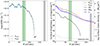Fig. 1.

Radial profiles for VCC 865 (NGC 4396). Left: sSFR profile (blue data points) with a smoothed profile shown as a black curve. The next five upper limits (where no Hα is detected but stellar mass is) are shown as blue arrows, connected by a dot-dashed line. Right: Surface brightness profiles for Hα NB (black) and r-band emission (red), along with the Σ_* profile (blue). The dashed black profile shows the detection limit for the Hα profile. In both panels, the green vertical line shows the median SF disc edge, R_sSFR, and the shaded green band the uncertainty range based on the 16^th and 84^th percentiles computed using a Monte Carlo simulation with 1000 iterations. The vertical black line shows the expected edge, R_norm, of the galaxy and the shaded grey band uncertainty range based on the 16^th and 84^th percentiles of the Monte Carlo simulation.

3.1. Extraction of radial profiles

Our analysis relies on using radial sSFR profiles to determine the edge of the SF disc. The sSFR is determined using SFR and stellar mass surface density (Σ_SFR and Σ_*) profiles, which we obtained using g, r, and Hα surface brightness profiles.

3.1.1. Creating object masks

In order to properly extract SB profiles of our target galaxies, we needed to mask any contaminating stars or background galaxies. For each galaxy in VESTIGE, we cut a postage stamp around the object with a size of 10 r_e, i on each axis, where r_e, i are i-band effective radii coming from Sérsic profile and growth curve fitting performed on NGVS images (in the few case where r_e, i is unavailable from NGVS, we use r_e, i = 60″). We used the Python package PHOTUTILS (Bradley et al. 2021) to create object masks for our postage stamps. Since our galaxies span a wide range of sizes and luminosities and our data quality and depth pick up small structures and low-SB features, we found a single masking run would not suffice.

We chose to employ a ‘hot, cool, cold’ masking routine based on Galametz et al. (2013) and Sazonova et al. (2021). First, the images were passed through a 2D top-hat smoothing kernel with a size equal to 0.2R_e, i. For the ‘hot’ run, we used a very high detection threshold, small minimum area and a small amount of deblending to identify the brightest peaks in the image. The ‘cool’ run followed, where we used a low detection threshold, large area and strong deblending. Using these first two runs, we masked ‘cool’ regions that are far from the galaxy centre, and masked nearby ‘cool’ regions where a ‘hot’ peak was identified (this attempts to mask areas around saturated stars, for example), except for the central hot peak associated with the galaxy. Finally, we performed the ‘cold’ run, where we used the mask created in the previous step and performed one more detection run using a low threshold, no deblending and a minimum area of 20 pixels.

We found that this routine worked well based on a visual inspection of all masks. In certain cases where over- or under-deblending occurred, we re-ran the masking routine, altering certain parameters as necessary until a good mask was produced. We show a table of the PHOTUTILS parameters used in each run in Appendix A. For a more detailed explanation of the ‘hot, cool, cold’ masking technique, we refer the reader to Sazonova et al. (2021).

3.1.2. Radial surface brightness extraction

The next step in our analysis was to extract surface brightness profiles of VESTIGE galaxies in the g, r and Hα bands (μ_r, μ_g and μ_Hα). We used the non-parametric surface brightness extraction pipeline AUTOPROF (Stone et al. 2021). AUTOPROF is based on the work of Jedrzejewski (1987) but with addition of machine learning regularisation techniques. The software provides a full pipeline for background fitting, centroid finding, masking and surface brightness extraction, and is proven to be proficient is extraction of low-surface brightness features. We used the deep g-band images in our initial AUTOPROF run, and set the object centre to be the same as the optical positions used in Boselli et al. (2023a), determined with NGVS (Ferrarese et al. 2012). We ran AUTOPROF with a fixed isoband width of 10 pixels (1.87″); full width of band) and sampled linearly in increments of 10 pixels, applying the masks created, as is described in Sect. 3.1.1. AUTOPROF varies the ellipticity and position angles of the isophotes with each radial step as the shape of the galaxy changes. Since the structure of SF galaxies is complex, especially with high-resolution data, varying the ellipticity and position angle in this way provides a more accurate measure of the galaxy shape in each radial bin. We then used the AUTOPROF forced photometry method to force the extracted g-band profile onto the r-band and Hα images in order to obtain the same radial sampling, ellipticities and position angles in all three bands.

In the right panel of Fig. 1 we show radial SB profiles for the r-band in red and the NB Hα in black. The dotted black line shows the Hα detection limit based on the noise in the image and the size of our sampled annuli. Uncertainties on surface brightness values are computed by AUTOPROF dividing the inter-percentile range (between the 16^th and 84^th percentiles) by $2 \sqrt{N}$ $2\sqrt{N}$ where N is the number of pixels contributing to the SB measurement.

3.1.3. Stellar-mass surface density profiles

To obtain Σ_* profiles, we turned to the mass-to-light versus colour relations (MLCRs) calibrated in Roediger & Courteau (2015). These calibrations provide linear relations between colour and mass-to-light ratio (M_*/L)_λ for a given waveband, λ, based on either Bruzual & Charlot (2003) or Conroy et al. (2009) (FSPS) stellar population synthesis (SPS) models. It follows that

$\begin{matrix} log {(M_{*} / L)}_{λ} = m_{λ} \times (colour) + b_{λ} . \end{matrix}$ $\begin{aligned} \log {(M_*/L)_{\lambda }} = m_{\lambda } \times (\mathrm{colour}) + b_{\lambda }. \end{aligned}$ (1)

We chose to use λ = r, g − r colour and the Bruzual & Charlot (2003) SPS models with a Chabrier (2003) IMF, so m_λ = 1.629 and b_λ = −0.792 (see Table A.1 of Roediger & Courteau 2015). After calculating log(M_*/L)_r at each radial step from the g, and r-band SB profiles, we transformed our r-band SB profile into Σ_* using

$\begin{matrix} log Σ_{*} = log {(M_{*} / L)}_{r} + 0.4 (m_{abs, ⊙, r} - μ_{r}) + 8.63, \end{matrix}$ $\begin{aligned} \log {\Sigma _*} = \log {(M_*/L)_{r}} + 0.4\left(m_{\rm abs, \odot , r} - \mu _{r}\right) + 8.63, \end{aligned}$ (2)

where m_{abs, ⊙, r} = 4.64 (Willmer 2018) and Σ_* has units of M_⊙/pc². The right panel of Fig. 1 shows the Σ_* profile for VCC 865 in blue, using the secondary y axis on the right.

While Eq. (2) provides a convenient measure of stellar mass, it does not account for variations in dust content amongst individual galaxies. Larger-than-average dust leads to an underestimated luminosity, biasing the mass low. This is partially mitigated by the fact that the larger dust content also reddens the light, and therefore increases the mass-to-light ratio inferred from observed colours. The net effect is that there is a small, systematic uncertainty in our stellar mass profiles. Based on radial dust attenuation profiles from the Calar Alto Legacy Integral Field Area (CALIFA; Sánchez et al. 2012; González Delgado et al. 2015) and Mapping Nearby Galaxies at Apache Point (MaNGA; e.g. Bundy et al. 2015; Goddard et al. 2017; Greener et al. 2020), we expect that, in the most extreme cases, the radial variation in a dust profile is ±0.5 mag from the weighted average. Propagating this effect through Eqs. (1) and (2) shows that the attributed uncertainty on log(Σ_*) is ≲0.3 dex.

As a consistency check of our Σ_* profiles, we numerically integrated the Σ_* profiles out to R_norm (as defined in Sect. 3.2.2) to obtain the total stellar mass for the galaxy, and compared the results to the stellar masses obtained from SED fitting by Boselli et al. (2023a), finding good agreement, as is shown in Fig. 2. The mean difference in log-log space between our recovered stellar mass value and that measured in Boselli et al. (2023a) is 0.02 with a scatter of 0.21 after removing 3σ outliers. Our Σ_* profiles are corrected for inclination such that each profile describes a face-on galaxy, allowing consistent determination of galaxy edges based on critical Σ_* value. We describe the inclination correction in Appendix B.

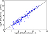Fig. 2.

Recovered total stellar masses obtained by numerically integrating Σ_* profiles up to R_norm compared to stellar masses obtained by Boselli et al. (2023a) through SED fitting.

3.1.4. Star formation rate profiles

To transform Hα SB profiles into SFR surface density (Σ_SFR) profiles, we used the calibration of Calzetti et al. (2010) (which assumes solar metallicity and constant SFR) modified to include a Chabrier IMF (Chabrier 2003), as in Boselli et al. (2023a). This model produces the relation

$\begin{matrix} SFR [M_{⊙} {yr}^{- 1}] = 5.01 \times 10^{- 42} L (H α) [erg s^{- 1}] . \end{matrix}$ $\begin{aligned} \mathrm{SFR}\,[\mathrm{M_{\odot }\,yr^{-1}}] = 5.01 \times 10^{-42} L (\mathrm{H\alpha })[\mathrm{erg\,s^{-1}}]. \end{aligned}$ (3)

Hα luminosities were determined based on the distance to the subcluster regions to which each galaxy belongs, based on the classifications in Section 2.4. We did not apply corrections for internal dust attenuation or [N II] contamination. Global corrections would not alter the shape of the radial profiles being studied, and deriving spatially resolved dust attenuation curves is beyond the scope of this work. As a check that dust corrections are not necessary for our results, we applied spatially resolved attenuation corrections (A_Hα as a function of radius) from CALIFA (Sánchez et al. 2012; González Delgado et al. 2015) and MaNGA (e.g. Bundy et al. 2015; Goddard et al. 2017; Greener et al. 2020) to a subset of our galaxies and re-ran our algorithm for finding R_sSFR. We found no changes in our measured R_sSFR, showing that typical dust gradients would have no effect on our measured values.

3.2. Quantifying the degree of truncation

We measured the edges of the SF discs of VESTIGE galaxies by identifying a turn-off point in their sSFR profiles, as is described in detail below (Sect. 3.2.1). In order to determine how truncated VESTIGE SF discs are relative to the field, we would ideally measure the edges of SF discs from an isolated field sample matched on colour and stellar mass. However, the VESTIGE sample does not extend beyond the Virgo cluster environment, and existing large Hα field samples have comparatively shallow depths. Instead, we compared our SF disc sizes to the expected sizes of discs based on the field sample of C22. At least for massive galaxies on the SFMS, C22 show that the optical edge corresponds to the edge of the SF disc, evidenced by breaks in the UV profile. We describe this process in more detail in Sect. 3.2.2.

3.2.1. Measuring the edge of the star-forming disc

We take inspiration from the methods of C22 who determined the edges of galactic discs by looking for breaks in surface brightness and optical colour profiles. Combining our constructed SFR and stellar mass density profiles, we calculated specific star formation rate (sSFR) profiles determined by

$\begin{matrix} sSFR (r) = \frac{SFR (r)}{Σ_{*} (r)} \cdot \end{matrix}$ $\begin{aligned} {\mathrm{sSFR} }(r) = \frac{\mathrm{SFR}(r)}{\Sigma _*(r)}\cdot \end{aligned}$ (4)

Uncertainties on the sSFR profiles were determined by compounding the uncertainties associate with the SFR and Σ_* profiles. Because the Σ_* profiles are so precisely defined, the uncertainties on the sSFR values are typically small relative to even local variations in the sSFR profile.

For disc galaxies on the SF main sequence (SFMS), sSFR profiles are shown to be flat for galaxies with M_* < 10^10.5 M_⊙ (the majority of our sample), with central suppressions in massive SF galaxies (e.g. Belfiore et al. 2018). This makes it straightforward to identify a drastic change in the shape of the profile, which signifies a change in the SFR distribution relative to the underlying stellar mass distribution. This means that features such as inner disc breaks will not be captured unless they correspond to a SF disc edge, as desired.

We then defined R_sSFR as the last local maximum in the sSFR profile before it drops off, ignoring small peaks that may occur while the sSFR profile is dropping off. Because VESTIGE imaging has high-resolution, our profiles are sensitive to small structures across the galaxy. We chose to smooth our profiles with a 1D Gaussian filter with σ = 1 to reduce the risk that a peak due to small-scale structure is determined to be the turn-off point. In certain extreme cases, galaxies were found to have centralised star formation when visually inspected. This observation results in a very truncated disc according to our criteria, though the sSFR profile may not have any detectable local maxima. Thus, we added a condition in our algorithm to check if the sSFR profile falls by at least 1 dex over the range of radii for which sSFR values are measured. If this is the case, we identified the smallest radial value as the edge of the SF disc (R_sSFR = 2.805″).

In Fig. 1, R_sSFR is shown with its associated uncertainty range (Sect. 3.2.3) as a green band and dashed green line. In this example, R_sSFR clearly corresponds to a the location where a sharp decline in the sSFR profile begins. While there is still non-negligible star formation beyond this radius, the large change in slope represents a well-defined edge. We show the equivalent of Fig. 1 for eight total galaxies of varying stellar mass in Fig. E.1. In some galaxies (e.g. first example in Fig. E.1) the drop in sSFR is even more severe, with no detectable star formation beyond R_sSFR.

There exists in the literature many different methods for detecting features such as disc breaks that in some cases may correspond with the SF disc edges that we measure (e.g. Hunter & Elmegreen 2006; Herrmann et al. 2013, 2016). While beyond the scope of this paper, a study comparing the features identified by these different methods and the physical interpretations of each would be an interesting future work.

3.2.2. Determining the expected edges of galaxies

We wished to define an ‘expected’ edge for isolated counterparts to our cluster galaxies. We wanted to define this edge in a way that is insensitive to properties of the Virgo galaxies, such as colour profiles, which may be affected by environment. Therefore, we defined R_norm, the edge of the optical disc for an unperturbed galaxy of a given stellar mass, by first fitting a piecewise function to the Σ_*(R_edge) versus M_* relation from C22 to find the critical Σ_* value for a galaxy of a given stellar mass. This function is

$\begin{matrix} Σ_{*} (R_{edge}) = {\begin{matrix} 0.6, & log (M_{*}) < 9.6 M_{⊙} \\ 10^{(0.3 log (M_{*}) - 3.1)}, & log (M_{*}) \geq 9.6 M_{⊙} \end{matrix}, \end{matrix}$ $\begin{aligned} \Sigma _*(R_{\rm edge}) = \left\{ \begin{array}{ll} 0.6,&\log {(M_*)} < 9.6\,\mathrm{M_{\odot }}\\ 10^{\left(0.3\log {(M_*)} - 3.1\right)},&\log {(M_*)} \ge 9.6\,\mathrm{M_{\odot }} \end{array},\right. \end{aligned}$ (5)

where Σ_* has units of M_⊙ pc⁻². Using inclination-corrected Σ_* profiles, we determined R_norm by finding the point at which the profile drops below the threshold Σ_* value. In Fig. 1 we show R_norm as a black line with a grey band for its uncertainty. Figure 9 of Chamba et al. (2022) shows the ratio between R_edge to the effective radius as a function of stellar mass. The ratio is ∼4 for all stellar masses but contains significant scatter, stemming from the tighter size-mass relation that is produced when using R_edge.

3.2.3. Quantifying uncertainties

The measurement of R_sSFR is sensitive to the noise in the sSFR profile, the radial bin size, and the presence of small local maxima in the sSFR profile. Similarly, R_norm is sensitive to the noise in the Σ_* profile and the radial bin size. To quantify the uncertainties in these measurements, we performed a Monte Carlo simulation with 1000 iterations for each galaxy. During each iteration, we drew sSFR values for each radial bin from a Gaussian centred on the calculated values with a scale equal to the measured noise. We then ran the algorithm for finding the turn-off point, as is described in Sect. 3.2.1, and drew the final value for R_sSFR from a uniform distribution spanning the width of the radial bin. For each iteration, we also drew the Σ_* values in each radial bin from a Gaussian centred on the measured value and with a width equal to the noise. The Σ_* threshold value has an associated uncertainty from our piecewise fit to the C22 relation, so we also drew that value from a Gaussian distribution centred at the measured value with a width equal to the uncertainty. We then determined R_norm, which we again drew from a uniform distribution equal to the width of the radial bin. With 1000 values for both R_sSFR and R_norm, we had 1000 values for the ratio between the two and chose the accepted value to be the median and used the 16^th and 84^th percentile values as the upper and lower limits on the error.

Fig. 3 shows Hα and r-band imaging for VCC 865, with ellipses outlining R_sSFR and R_norm. We show eight total galaxies spanning a range of stellar masses in Fig. F.1. The ellipticities and position angles used for these ellipses are the local values determined by AUTOPROF at those radial points. On the right-hand side of the postage stamps are the sSFR profiles for these galaxies, again highlighting R_sSFR and R_norm. On the sSFR plots, we have included the upper limits of sSFR (based on Hα detection limits) for the next five radial bins in which Hα is not detected (but stellar mass is). This helps to highlight cases where, even in the absence of an obvious local peak to define R_sSFR, an edge is still clearly present.

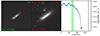Fig. 3.

Continuum-subtracted Hα emission (left), r-band optical emission (centre), and sSFR profile (right) for VCC 865 (NGC 4396). In the left and centre postage stamps, the green ellipse outlines R_sSFR while the red ellipse outlines R_norm. On the sSFR plots (right), we show R_sSFR and its associated uncertainty range as a green vertical line and band, and R_norm and its uncertainty range as a grey vertical line and band. Also included are the upper limits (down arrows) in the next five radial bins in which Hα is not detected (but stellar mass is); this represents the upper limit to the sSFR based on the Hα detection limits.

Figs. E.1 and F.1 display the variety of shapes that sSFR profiles exhibit due to local peaks of star formation or off-centre star formation, and show the success of our algorithm at detecting a physical R_sSFR in each of these cases. This success is validated by the green ellipses on the continuum-subtracted Hα images, which capture the Hα emission of the galaxies very well.

3.3. Final sample of galaxies

The full VESTIGE sample consists of 384 Virgo galaxies with Hα emission. We have removed a subset of galaxies from our sample based on the following criteria:

Three massive elliptical galaxies with Hα emission (M84, M86, M87).
Six additional faint galaxies for which the AUTOPROF routine did not produce good surface brightness profiles.
22 additional galaxies with fewer than three data points in their measured sSFR profile.
18 additional galaxies for which R_sSFR is clearly unphysical based on inspection of radial profiles (Appendix C).

In total, we have removed 49 galaxies, leaving us with a sample size of 335 down to M_* ≃ 10⁷ M_⊙.

4. Results

4.1. Galaxy size as a function of stellar mass

We first consider the size-stellar mass relation of our sample using R_norm and R_sSFR as our measurements of size, shown in Fig. 4. This puts our R_norm measurements in context with the results of C22. Fitting a linear relation to the log-log size-stellar mass relation, we find a slope of 0.33 ± 0.01 with a scatter of 0.16. This is similar to the fits of C22 who found slopes of 0.31 ± 0.01, 0.27 ± 0.02 and 0.32 ± 0.03 (with scatter of ∼0.1) when fitting their whole sample, giant spirals and dwarf SF galaxies, respectively. We find that our R_norm measurements are systematically smaller than the C22 R_edge values by ∼10%. In contrast, Chamba et al. (2024) found that Fornax cluster galaxies are ∼50% smaller than isolated galaxies, as R_edge (defined in the same way as C22) occurs at a higher stellar mass surface density. This is expected in the case where cluster galaxies have had their SF discs truncated. This justifies our use of the field-derived critical mass density for determining R_norm.

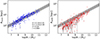Fig. 4.

Size-stellar mass relations. Left: Size-stellar mass relation for galaxies with identified R_norm. We fit a linear relation to the data and show that a slope of m = 0.34 ± 0.01 is measured, consistent with C22. The shaded grey region shows the 1σ scatter in the linear relation. Right: Size-stellar mass relation using R_sSFR, showing the linear fit to the R_norm-mass relation.

The relationship between R_sSFR and stellar mass does not follow a clear linear relation and has much more scatter than the size-mass relation with R_norm. This is expected in the case where galaxies with R_sSFR < R_norm are undergoing quenching mechanisms that may be mass-dependent.

We plot R_sSFR/R_norm against stellar mass in Fig. 5. Galaxies of all masses tend to have R_sSFR/R_norm < 1. There is a trend whereby galaxies with lower stellar masses have smaller values of R_sSFR/R_norm on average, though there is much scatter. Shown in grey bands are the detection limits based on our methods. The first results from our removal of any galaxies whose sSFR profiles contained fewer than three data points (R_sSFR = 6.545″). The second detection limit is at the radius for the first data point in the profiles, R_sSFR = 2.805″, since any galaxy could have a measured edge at the first data point.

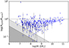Fig. 5.

R_sSFR/R_norm as a function of stellar mass. The two shaded grey regions show limits on the measurements of R_sSFR/R_norm. We have excluded any galaxies where the sSFR profile spans fewer than three data points, so the dashed black line has R_sSFR = 6.545″. In principle, any sSFR profile with more than three data points could still have a truncation at the first data point, so the dash-dotted line has R_sSFR = 2.805″. In both cases, R_norm is determined from the size mass relation in Fig. 4 at a distance of 16.5 Mpc.

4.2. R_sSFR/R_norm as a function of environmental indicators

In Fig. 6 we plot R_sSFR/R_norm as a function of both H I-deficiency and distance from the SFMS (determined in Boselli et al. 2023a). On the H I-deficiency plot we indicate which galaxies are on/above the SFMS and which are below. Similarly on the SFMS plot we indicate which galaxies are H I-normal and which are H I-deficient. While most H I-normal galaxies are on the SFMS, the converse is not true: many galaxies on the SFMS are H I-deficient. We observe that most galaxies have R_sSFR/R_norm < 1 regardless of H I content or SFR. Galaxies that are more H I-deficient or that are below the SFMS have more substantially truncated discs. Even for many galaxies on the SFMS, however, we find that R_sSFR/R_norm < 1. We interpret the ubiquity of truncated discs across the range of H I-deficiency and distance from the SFMS as evidence that nearly all Virgo galaxies are truncated relative to the field. For galaxies on the SFMS with normal gas content, the data points scatter around R_sSFR/R_norm ∼ 0.8. While we expect that even the most normal galaxies in our sample may be somewhat affected by the Virgo environment, without a direct field comparison we cannot say for certain that galaxies with 0.8 < R_sSFR/R_norm < 1 are truncated with respect to the field. Being mindful of this caveat, in further analysis we focus on galaxies with R_sSFR/R_norm < 0.8 We shall further discuss these results in context in Sect. 5.

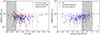Fig. 6.

R_sSFR/R_norm against star formation indicators. Left: R_sSFR/R_norm as a function of H I-deficiency, with galaxies located on or above the SFMS shown in red and galaxies below the SFMS shown in blue. The range of H I-normal galaxies is shaded. Right: R_sSFR/R_norm as a function of distance from the SFMS, with H I-normal galaxies shown in red and H I-deficient galaxies shown in blue. The SFMS is shown as a shaded region.

A peculiar feature in Fig. 6 is the handful of galaxies that are extremely H I-deficient (H I-def > 2.5) and well below the SFMS with only mildly truncated discs. Upon inspection, some of these galaxies appear to be starbursts and feature low-SB ionised gas emission stemming from a central burst of star formation. Our measure of disc truncation is not able to pick these galaxies out, however they do not really have SF discs anymore at all. We show an example in Appendix C.

4.3. R_sSFR/R_norm across the Virgo environment

The Virgo cluster is made up of a main cluster (Cluster A), along with another large structure (Cluster B) and several smaller substructures outlined in Table 1. Throughout our discussion of the main cluster structure, we adopt the NFW model of Simionescu et al. (2017) to describe the mass profile of the cluster. This fit infers R₂₀₀ = 0.974 Mpc.

The footprint of the Virgo cluster with its substructures is shown in Fig. 7. Each galaxy is shown at its 2D position in the cluster region, with the data points sized according to the stellar mass of the galaxy and coloured according to the value of R_sSFR/R_norm The radii of the circles depicting different substructures are those listed in Table 1. We use a discrete colour mapping on Fig. 7 to separate galaxies into three categories based on their values of R_sSFR/R_norm. Blue data points have R_sSFR/R_norm > 0.8 and are considered at most mildly truncated. Since we have not used a control sample to directly determine the scatter in R_sSFR/R_norm for normal SF galaxies, we do not focus on these mildly truncated galaxies in our analysis. Yellow data points (0.3 < R_sSFR/R_norm ≤ 0.8) are considered moderately truncated and red points (R_sSFR/R_norm ≤ 0.3) are considered extremely truncated. We can see from Fig. 7 that there are groupings of galaxies with at least moderately truncated discs in the M and Low-Velocity clouds, as well as in and around the W and W′ cloud regions. If these galaxies are truly a part of these substructures, this result indicates the possible importance of pre-processing in group structures beginning to perturb galaxies before they fall into the main cluster. We assign galaxies to their most likely substructure as outlined in Sect. 2.4. In Fig. 8 we show a box-and-whisker plot displaying the median and interquartile range of R_sSFR/R_norm for five groupings of Virgo substructures: all regions, Cluster A alone, Cluster B alone, the W and W′ clouds together, and the M cloud, low-velocity cloud and Cluster C together. In each grouping, the median value of R_sSFR/R_norm is less than unity, with the scatter varying across the groupings.

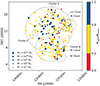Fig. 7.

Right ascension and declination footprint of VESTIGE galaxies with measured values of R_sSFR/R_norm. Overplotted are the seven identified regions associated with the Virgo cluster: Clusters A, B and C, the W and W′ clouds, the M cloud and the Low-Velocity cloud, with the radii noted in Table 1. Data points are sized proportionally to the stellar mass of the galaxy, and coloured based on the value of R_sSFR/R_norm.

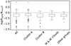Fig. 8.

Box-and-whisker plot showing the median and first and third quartiles of the distributions of R_sSFR/R_norm in the entire sample and four groupings of Virgo cluster substructures. ‘Other groups’ covers the M and low-velocity clouds as well as Cluster C.

We also look at the distribution of galaxies in projected phase-space (PPS) in Fig. 9. To do so, we plot the radial velocities of galaxies (as collected in Boselli et al. 2023a) relative to the cluster against the 2D distance from the cluster centre (M87). While PPS diagrams often normalise the x axis by R₂₀₀ and the y axis by the velocity dispersion (σ), we use physical (unnormalised) coordinates to ensure our interpretation of the results is not sensitive to the assumed value of R₂₀₀ and σ. The data points are colour-coded according to R_sSFR/R_norm, as in Fig. 7. Evidence of truncations can be found throughout the cluster, including in the area beyond the virial radius of 0.974 Mpc. Interestingly, we do not find a strong trend between degree of truncation (based on the colours of the data points) and location in PPS. This contrasts sharply with the distribution of quenched galaxies relative to star forming galaxies, illustrated as the background greyscale shading. This is created by comparing the 2D kernel density estimation (KDE) of the VESTIGE Hα sample distribution to that of the full NGVS sample, for the mass range M_* > 10⁸ M_⊙ where NGVS is mostly redshift complete.

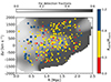Fig. 9.

PPS diagram of VESTIGE galaxies with VESTIGE Hα detection fractions computed using the ratio of 2D Gaussian KDEs of the VESTIGE and NGVS distributions. Data points are sized proportionally to the stellar mass of the galaxy, and coloured based on the value of R_sSFR/R_norm. While the detection fractions show the expected structure, truncated discs exist across the cluster environment.

As was expected, the VESTIGE detection fractions are lower in regions of phase space near the centre of the cluster and with lower velocities, corresponding to ancient infall regions where galaxies have interacted with the cluster environment likely on multiple passes through the centre. If these ancient infallers have quenched, we would not expect detectable Hα emission and thus they are absent from the VESTIGE sample. On the contrary, the VESTIGE detection fractions are highest in the infall regions of the cluster, at higher relative velocities and far from the centre.

5. Discussion

5.1. Modelling the radial profiles of galaxies

In this section we model the radial stellar and gaseous components of a normal SF galaxy (prior to any quenching) and explore how they change under two different simple quenching models. Starting with a chosen stellar mass, we use the scaling relations of Huang et al. (2012) to obtain an H I mass and integrated SFR for our galaxy. With the relations from Sect. 3, we obtain the critical Σ_* value and edge radius (R_norm; R_sSFR at t = 0) of our galaxy. This allows us to determine the scale radius for an exponential Σ_* profile. For simplicity, we assume that the SFR profile will have the same scale radius, though in practice the scale radii for the two components could differ. Following the sub-kiloparsec Kennicutt-Schmidt law of Bigiel et al. (2008), the SFR profile of the model galaxy is proportional to the H₂ profile. The H I profile is flat at 8 M_⊙ pc⁻², which is a good approximation based on the observations of Bigiel et al. (2008).

Observations comparing gas density profiles and Hα profiles have identified that breaks in Hα profiles correspond to a critical gas density for star formation (e.g. Kennicutt 1989), which can signify the edge of the SF disc. Additionally, through our analysis we have used R_norm to define the expected edge of the SF disc for a normal, isolated galaxy. By incorporating the critical gas threshold for star formation, our SFR (and therefore H₂) profiles drop off abruptly at R_norm, where R_sSFR = R_norm at t = 0 and the threshold gas density is the value of the total gas density at R_norm at t = 0. The stellar mass surface density profile also has a break at R_norm. However, unlike R_sSFR, the location of this break will not change as we evolve the model.

In our simple model, the break at the gas density threshold is abrupt, with no star formation occurring beyond this radius; in reality, galaxy disc edges are less drastic due (for example) to localised peaks of dense gas fuelling small amounts of star formation in the outer disc. This simplification does not change our results as our goal is to explore how R_sSFR changes with time in different quenching scenarios. As gas is consumed and/or removed from the galaxy, the total gas density will decrease, causing the position of R_sSFR to change.

5.2. Ram-pressure stripping

The effects of RPS are known to be present in the Virgo cluster based on studies of individual or small samples of galaxies that display evidence of stripped H I gas through direct observations of the H I (e.g. Gavazzi et al. 2001; Kenney et al. 2004; Chung et al. 2007; Sorgho et al. 2017; Minchin et al. 2019; Boselli et al. 2023c) or observations of radio emission (e.g. Vollmer et al. 2004, 2010, 2013; Vollmer & Huchtmeier 2007; Crowl et al. 2005; Chyży et al. 2007; Kantharia et al. 2008) or ionised gas (e.g. Yoshida et al. 2002; Boselli et al. 2016, 2018b, 2021; Fossati et al. 2018) in the stripped material. A multitude of simulation studies have shown that RPS can deplete the gas reservoir of a galaxy on timescales of < 1 Gyr (e.g. Vollmer et al. 2001; Boselli et al. 2006, 2016; Steinhauser et al. 2016; Fossati et al. 2018; Junais et al. 2022). However, substantial removal of SF gas may not occur until the galaxy approaches first pericentre as the combination of a dense ICM and high relative speeds are necessary to remove gas from a deep galactic potential well. Other high-resolution simulations have shown that while removal of the SF gas is rapid, removal of the entire gas reservoir may require timescales of > 1 Gyr (e.g. Tonnesen et al. 2007).

Additionally, the multi-phase nature of gas plays a role in the efficiency of stripping, with denser gas being harder to strip (e.g. Tonnesen & Bryan 2009). Our simple model below neglects any direct stripping of the molecular gas and assumes that H₂ depletion occurs only through star formation. Once the H I gas is entirely removed after a stripping event, the H₂ gas cannot be replenished. In fact, stripping of molecular gas has been shown to occur in Virgo (Watts et al. 2023). Factoring this into our model would only serve to speed up the RPS timescales, which will not affect the interpretation of this model since the RPS timescales are much faster than starvation-only models.

To explore the range of effectiveness of RPS throughout the cluster, we invoke a simple model to determine where the combined ICM density and galaxy velocity becomes large enough to overcome the gravitational restoring force holding the gas in the galactic disc. Using a M_* = 10^9.5 M_⊙ model galaxy, we can calculate the restoring force from each component. While previous works have considered only the stellar disc component of the restoring force acting to hold the H I gas (e.g. Yoon et al. 2017; Boselli et al. 2022), we loosely follow Roberts et al. (2019) and consider the force from the stellar disc, dark matter halo, and the self-gravity of the gas itself². Therefore, the restoring force is given as

$\begin{matrix} f = [g_{*} (r) + g_{H i} (r) + g_{H_{2}} (r) + g_{DM} (r)] Σ_{H i} (r), \end{matrix}$ $\begin{aligned} f = \left[g_*(r) + g_{\mathrm{H}i }(r) + g_{\rm H_{2}}(r) + g_{\rm DM}(r)\right]\,\Sigma _{\mathrm{H}i }(r), \end{aligned}$ (6)

where g_*(r), $g_{H I} (r)$ $g_{\mathrm{H}\textsc{i}}(r)$ , g_H₂(r) and g_DM(r) are the contributions to the gravitational acceleration from the different galactic components (stars, H I, H₂ and dark matter) and $Σ_{H I} (r)$ $\Sigma_{\mathrm{H}\textsc{i}}(r)$ is the surface density of H I gas. We leave further details of the model to Appendix D.

Ram-pressure is determined by ρ_ICMv², where ρ_ICM is the density of the ICM and v is the relative velocity of the galaxy within the cluster. We can then calculate the strength of the ram-pressure at any point in phase space. We assume that a galaxy with some observed radial velocity, v_r, has a three-dimensional velocity $v = \sqrt{3} v_{r}$ $v = \sqrt{3}v_{\mathrm{r}}$ , since the ram-pressure depends on this three-dimensional velocity through the ICM. While this factor is statistically sound for a population of galaxies on isotropic orbits, the orbits of individual galaxies may vary. A more realistic analysis of the ram-pressure experienced by infalling Virgo galaxies was reviewed by Boselli et al. (2022), using a simulation to characterise accurate orbital parameters.

With this model, we can calculate whether the ram-pressure at a given 2D point in projected phase space is sufficient to overcome the restoring force of the galaxy at a given galactocentric radius. We show a second PPS diagram in Fig. 10, where the x- and y-axes are the same as in Fig. 9. The two dashed black curves on the plot indicate the escape velocity of the cluster based on the potential from the Simionescu et al. (2017) NFW profile. Also plotted are, for a M_* = 10^9.5 M_⊙ galaxy modelled as in Section 5.1, the lines in phase space where the ram-pressure from the ICM can strip gas from the optical edge (R_norm) of the galaxy (red), from 0.5 R_norm (amber) and from the centre (0.01 R_norm; green). The data points on Fig. 10 are galaxies previously identified to be undergoing RPS (Boselli et al. 2022 and references therein). These galaxies have a wide range of H I-deficiencies and are located across the cluster environment; however, the most perturbed galaxies are preferentially located closer to the cluster centre, and at high relative velocities, near the contours where we expect a significant fraction of gas to be stripped from galaxies on typical orbits. There are also several galaxies undergoing RPS that are located beyond the red contours, where our model predicts ram pressure is typically not effective. This is unsurprising, as the strength of RPS on individual objects depends on the shapes of orbits and the exact radial profiles of the galactic components, which can differ significantly from our statistical model assumptions.

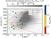Fig. 10.

PPS diagram showing the region within the escape velocity of the cluster as the region between the two dashed black lines. The escape velocity is determined based on the NFW profile of Simionescu et al. (2017). The green, yellow, and red lines show the contours where a M_* = 10^9.5 M_⊙ galaxy could have its gas removed by RPS from 0.01, 0.5, and 1 R_norm, respectively, assuming isotropic orbits. Data points are sized proportionally to the stellar mass of the galaxy, and coloured based on the value of R_sSFR/R_norm. The background greyscale shows the phase-space number density of galaxies with 0.3 < R_sSFR/R_norm < 0.7 determined using a 2D Gaussian KDE.

The background greyscale of Fig. 10 shows the phase space number density of galaxies with moderate truncations (0.3 < R_sSFR/R_norm < 0.8), determined using a 2D Gaussian KDE. A dense region of truncated discs is located just outside the virial radius (between 1 and 1.5 Mpc) and with relative velocities between 0 and 1500 km s⁻¹. Statistically, many of these galaxies are likely to be on their first infall based on their location in phase space (Rhee et al. 2017). This region of phase space can also contain backsplash galaxies. However, if the galaxies in our sample had already passed through the densest region of the ICM in the cluster centre they likely would have been completely stripped due to RPS. In fact, we find the quenched fractions to be lower in these regions (Fig. 9), again supporting that many of these galaxies are likely on their first infall into the cluster. While RPS may still be effective for some galaxies in this region of PPS, depending on their precise orbital geometries and restoring forces, the ubiquity of truncated discs in these regions suggests other effects may also be at play.

5.3. Starvation

In a simplified steady-state scenario, a galaxy forms stars from molecular gas that is replenished by atomic gas, which is in turn replenished by hot gas that has accreted from the cosmic web onto the galactic halo. If accretion of gas ceases (e.g. Larson et al. 1980) or halo gas is removed via stripping (‘harassment’: Moore et al. 1996, 1998) when the galaxy becomes a satellite of a more dominant system, the galaxy will eventually exhaust its reservoir of both atomic and molecular gas through star formation and become quenched. As such, starvation is typically thought of as a process that uniformly lowers the gas density and suppresses star formation across the galactic disc, producing an anaemic, but not necessarily truncated, disc (e.g. Boselli et al. 2006). However, starvation models typically do not account for observations that suggest that there is a critical total gas density threshold required to fuel local star formation. We show below that a simple starvation model that factors in a gas density threshold for star formation will, in time, produce a galaxy with a truncated disc.

We demonstrate this with a simple toy model: At t < 0 (where t = 0 is the time at which starvation begins) a galaxy is in a ‘steady state’ of gas accretion where the radial gas density profiles of atomic and molecular gas remain constant over time due to accretion of hot halo gas; this in turn fuels a constant Σ_SFR profile. The radial profiles for the galactic components are determined as outlined in Sect. 5.1. We then allow our model to evolve from t = 0. At this point, we assume the galaxy is completely unable to accrete fresh gas, and thus the H I reservoir cannot be replenished as it converts into H₂. The model assumes that as long as there is H I in the galaxy then the H₂ profile (and thus the SFR profile) will remain constant³. At each timestep, stars form from the H₂ gas and the H₂ is replenished by the H I. Once the H I has been used up, subsequent star formation will deplete the remaining molecular gas, which will in turn reduce the SFR, moving the galaxy off of the main sequence.

In Fig. 11 we show the evolution of the total gas density profile in this model, for a M_* = 10^9.5 M_⊙ galaxy over 8 Gyr of starvation. Also plotted is the threshold gas density for star formation. Therefore, the points where the red line crosses each black curve are the points where the galaxy would be truncated at each timestep. In this model, while starvation takes a long time to move a galaxy off the SFMS and completely deplete its gas reservoir (as is shown in Appendix D), moderate truncation can still happen after just 1−2 Gyr. While this model is based on oversimplified assumptions about the gas distribution, consumption, and redistribution, as a toy model it effectively illustrates that any model of starvation that globally reduces the total gas density profile will also truncate the SF disc, if a critical gas threshold for star formation is included.

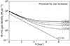Fig. 11.

Evolution of total gas density (Σ_HI + Σ_H2) over 8 Gyr for a $M_{*} = 10^{9.5} M_{⊙}$ $M_* = 10^{9.5}\,\mathrm{M}_{\odot}$ galaxy undergoing simple starvation. The threshold gas density for star formation (explained in Appendix D) is shown as a dashed red line. By the t = 8 Gyr curve, all H I gas has been consumed and as such the H₂ is not being replenished, causing the total gas density to decrease at all radii.

Quantitatively, these results will depend on the treatment of starvation in the model, and also on the stellar mass of the galaxy, but qualitatively the behaviour would remain the same. In future work a gas threshold for star formation should be incorporated into a more sophisticated model, like the chemo-spectophotometric model of Boselli et al. (2006). Such a model should then be tested in order to see if it can also re-produce observed colour and metallicity gradients in galaxies.

5.4. Ram-pressure stripping and starvation in context

In Fig. 12 we show a representation of the effects on R_sSFR and H I content of our starvation model compared to our RPS+starvation model for a galaxy falling radially into the cluster. Previous studies have indicated that starvation and removal of hot halo gas can be efficient as far out as 5R₂₀₀ in clusters (e.g. Bahé et al. 2013). While we have not directly modelled the halo gas removal here, we assume for simplicity that starvation begins at 2R₂₀₀, at which point the galaxy can no longer accrete fresh gas from the cosmic web. This choice of starting point is not meant to predict exactly where or how starvation begins for individual galaxies, but rather to show how starvation onset beyond R₂₀₀ produces galaxies with truncated discs before ram-pressure is sufficient to strip gas directly from the galactic disc.

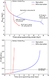Fig. 12.

Evolution through time of R_sSFR (top) and H I-deficiency (bottom), for a M_* = 10^9.5 M_⊙ galaxy undergoing a simple starvation model (blue curves) and a galaxy falling into Virgo radially and experiencing RPS along with starvation (red curves). The horizontal dashed black line at H I-def = 0.4 represents the point above which a galaxy is considered H I-deficient.

For a M_* = 10^9.5 M_⊙ galaxy in our model, it takes ∼1.3 Gyr for the galaxy to fall radially from 2R₂₀₀ to R₂₀₀, during which time the size of the SF disc shrinks significantly, by a factor of ∼2. In the absence of any ram pressure stripping or other effects, the disc would continue to shrink gradually for several gigayears, as shown by the blue line. However, for this galaxy on a radial orbit our model predicts RPS begins at t ∼ 1.8 Gyr, when the galaxy is at ∼0.5R₂₀₀, and is the dominant quenching force until t ∼ 1.95 Gyr. This rapid timescale (∼150 Myr) for RPS is broadly consistent with the findings of other recent studies (e.g. Boselli et al. 2006, 2021; Fossati et al. 2018). At this point, when R_trunc = 3.1 kpc, the H₂ gas becomes dominant in the gas profile, and shortly after the remaining H I gas from the galactic centre is removed by RPS. Once the galaxy is completely H I-deficient, the consumption of H₂ takes over and slowly truncates the disc further, moving it off the main sequence as the SFR decreases with decreasing H₂ content⁴.

This shows that there is the potential for a galaxy to become completely stripped of H I by its first pericentre approach in the cluster. The removal of H I by RPS is most pronounced near the cluster centre, however, which makes our starvation model a natural choice to explain galaxies near and beyond R₂₀₀ that appear to be on first infall with already-truncated discs.

Our toy model indicates that, while starvation has a long timescale to completely quench a galaxy, it may contribute to considerable disc truncation in only 1−2 Gyr. This means a galaxy can already have a truncated disc before RPS becomes dominant, especially if starvation begins early, when the galaxy is well beyond the virial radius. This implies a ‘slow-then-rapid’ quenching sequence, whereby galaxies begin slow quenching via starvation and, at a critical point during first infall, RPS becomes dominant and rapidly quenches the galaxy. These findings are consistent with those of Roberts et al. (2019), who found that the quenched fraction of galaxies in nearby clusters increases sharply at a threshold ICM density corresponding to the point where galaxies are susceptible to having the majority of their gas removed by RPS.

We argue that this slow-then-rapid quenching scenario is also consistent with the ‘delayed-then-rapid’ scenario of Wetzel et al. (2012). In our case, the early starvation quenching mode is the ‘delayed’ phase because it does not rapidly quench star formation in the galaxy. The global SFR and H I content of the galaxy do decrease during the time that starvation is dominant (∼1.8 Gyr), but slowly enough that the integrated SFR drops by only ∼10% (∼0.07 M_⊙ yr⁻¹ for the modelled galaxy in Fig. 12). This means the galaxy would remain on the SFMS during the starvation phase, according to the main sequence fit defined in Boselli et al. (2023a).

We find this to be an attractive model to explain the dense region of moderately truncated discs beyond the virial radius of the main cluster as is seen in Fig. 10. The galaxies in this region have a range of H I-deficiencies and SFRs. The precise effects of starvation on the global gas content and SFR will depend on the details of the starvation mechanism and the time since starvation onset. Galaxies of different stellar masses will experience qualitatively the same effects, though the timescales may vary due to differences in gas content and SFR. While reproducing the parameters of individual galaxies is beyond the scope of this work, the peculiar trends seen in Fig. 6 can be qualitatively explained with this model. In Fig. 6, galaxies with moderate truncations can be seen with only mild H I-deficiencies and on the SFMS. Additionally, while SFMS galaxies are scattered across the range of H I-deficiencies, most H I-normal galaxies are on the SFMS. A slower process such as starvation truncating a disc, removing H I gas and then moving a galaxy of the main sequence successively over long timescales explains these trends since there is a high chance of observing a given galaxy in one of these three stages. Starvation before R₂₀₀ could occur when a galaxy is a part of a smaller substructure, providing an explanation for the large number of truncated discs seen in the cloud structures of Virgo (Fig. 7). Other pre-processing mechanisms such as gravitational effects and even RPS (shown to be present in some groups and smaller clusters: Roberts et al. 2021; Serra et al. 2023) could occur in these regions as well, and should be explored further with dedicated studies of pre-processing in Virgo substructures.

6. Summary and conclusions

We have used spatially resolved Hα imaging from VESTIGE, coupled with optical data from NGVS, to measure the edge of SF discs of galaxies across the entire footprint of the Virgo cluster, for M_* > 10⁷ M_⊙. To quantify the expected sizes of discs for isolated counterparts (R_norm), we have developed a methodology inspired by the physically motivated definition for the edge of a galactic disc outlined by Chamba et al. (2022). We have used AUTOPROF to measure surface brightness profiles in Hα, as well as the r and g bands, allowing us to construct Σ_* profiles and sSFR profiles. From our sSFR profiles, we have identified the turn-off point (R_sSFR) based on the derivative of the profiles. We summarise our key results below:

Disc truncations, where R_sSFR/R_norm < 1, appear ubiquitous across the Virgo cluster and as a function of stellar mass, H I-deficiency, and distance from the SFMS. However, we are cautious to assume that galaxies with minor disc truncations (R_sSFR/R_norm > 0.8) are truly truncated due to the lack of a control sample and the presence of SF, gas-normal galaxies with minor truncations (Sect. 3.2).
We find that moderate disc truncations are more common at lower stellar mass, greater H I-deficiency, and for galaxies that have fallen off the SFMS. However, these trends are not strong and contain considerable scatter (Figs. 5, 6). Chamba et al. (2024) measured the edges of galaxies using a method analogous to Chamba et al. (2022) and found that galaxies in the Fornax cluster are systematically smaller than field counterparts, with a similar trend in stellar mass to our findings.
Disc truncations occur to varying degrees across the entire cluster footprint, including in areas outside of the main cluster where galaxies may be infalling in groups (Fig. 7). The ubiquity of truncated discs across the cluster environment was also noted for the Fornax cluster by Chamba et al. (2024). We note as well that our sample consists only of galaxies with detectable Hα emission, most of which are therefore SF systems. This means that galaxies that are entirely quenched and would therefore have no measurable R_sSFR are not shown in our results. A comparison with galaxy densities from NGVS shows that the quenched fraction does indeed increases close to the cluster centre, so the truncated discs we measure are not representative of all galaxies in these regions (Fig. 9). This is consistent with results from Boselli et al. (2014b).
The high number of galaxies with moderately truncated discs in regions with low quenched fractions and low ICM density implies additional drivers giving a head-start to quenching before RPS becomes the dominant gas removal mechanism.
Galaxies on first infall may experience starvation before RPS, whether only in the main cluster or in smaller structures prior to cluster infall. We have shown that a starvation model can produce disc truncations when including a threshold gas density for star formation. Starvation beginning early, followed by a dominant RPS phase suggests a slow-then-rapid quenching sequence, consistent with the findings of Roberts et al. (2019). The nature of this quenching sequence is also broadly consistent with the delayed-then-rapid mechanism described in Wetzel et al. (2012), since the early starvation phase only mildly affects the integrated SFR of the galaxy before the RPS phase rapidly quenches it. Our results show that galaxies in the W and W′ Cloud regions have truncated discs, and a further study of group pre-processing prior to infall into the main Virgo cluster is critical to understanding the full evolutionary sequence of galaxies in these dense environments.

¹

The measurement is often termed as the ‘effective radius’ when determined with a Sérsic fit to a galaxy (de Vaucouleurs 1948; Sérsic 1963), while ‘half-light radii’ typically is used when the total flux of the galaxy has been determined and used to find the radius that contains half the flux.

²

Roberts et al. (2019) also factored in a bulge component of the stellar mass based on bulge-disc decomposition, but we model the stellar component of our galaxies as a disc only.

³

This prescription is likely an oversimplification as H I-deficient galaxies have been shown to have reduced star formation efficiency; (e.g. Villanueva et al. 2022; Brown et al. 2023).

⁴

We have not considered the effects of RPS on the H₂ in our model; if RPS also removed H₂ then the quenching of the galaxy in this final stage would be even more rapid.

Acknowledgments

We thank the anonymous referee for their constructive feedback that has helped us to greatly improve this manuscript. We are grateful to the whole CFHT team who assisted us in the preparation and in the execution of the observations and in the calibration and data reduction: Todd Burdullis, Daniel Devost, Bill Mahoney, Nadine Manset, Andreea Petric, Simon Prunet, Kanoa Withington. This research was supported by an NSERC Discovery grant to MLB. MB acknowledges support by the ANID BASAL project FB210003. J is grateful to the Polish National Science Centre grant UMO-2018/30/E/ST9/00082 and the Polish National Agency for Academic Exchange POLONIUM grant BPN/BFR/2022/1/00005. The preparation of this manuscript and much of the research behind it took place at the University of Waterloo, on the traditional territory of the Neutral, Anishinaabeg and Haudenosaunee peoples. The campus is located on the Haldimand Tract, the land granted to the Six Nations that includes six miles on each side of the Grand River. The authors from the University of Waterloo community acknowledge the privilege to work on these traditional lands. We also acknowledge that the data for this research was collected at CFHT on the summit of Mauna Kea, a location with great cultural significance to the Native Hawaiian community. Software. ASTROPY (Astropy Collaboration 2013, 2018, 2022), AUTOPROF (Stone et al. 2021), IPYTHON (Pérez & Granger 2007), MATPLOTLIB (Hunter 2007), NUMPY (van der Walt et al. 2011), PANDAS (McKinney 2010; Reback et al. 2020), PHOTUTILS (Bradley et al. 2021), SCIPY (Virtanen et al. 2020), TOPCAT (Taylor 2005).

References

Alberts, S., Adams, J., Gregg, B., et al. 2022, ApJ, 927, 235 [NASA ADS] [CrossRef] [Google Scholar]
Astropy Collaboration (Robitaille, T. P., et al.) 2013, A&A, 558, A33 [NASA ADS] [CrossRef] [EDP Sciences] [Google Scholar]
Astropy Collaboration (Price-Whelan, A. M., et al.) 2018, AJ, 156, 123 [Google Scholar]
Astropy Collaboration (Price-Whelan, A. M., et al.) 2022, ApJ, 935, 167 [NASA ADS] [CrossRef] [Google Scholar]
Bahé, Y. M., McCarthy, I. G., Balogh, M. L., & Font, A. S. 2013, MNRAS, 430, 3017 [Google Scholar]
Baldry, I. K., Balogh, M. L., Bower, R. G., et al. 2006, MNRAS, 373, 469 [Google Scholar]
Balogh, M. L., Morris, S. L., Yee, H. K. C., Carlberg, R. G., & Ellingson, E. 1997, ApJ, 488, L75 [NASA ADS] [CrossRef] [Google Scholar]
Balogh, M. L., Schade, D., Morris, S. L., et al. 1998, ApJ, 504, L75 [NASA ADS] [CrossRef] [Google Scholar]
Balogh, M. L., Navarro, J. F., & Morris, S. L. 2000, ApJ, 540, 113 [Google Scholar]
Balogh, M. L., McGee, S. L., Mok, A., et al. 2016, MNRAS, 456, 4364 [NASA ADS] [CrossRef] [Google Scholar]
Barnes, J. E. 2004, MNRAS, 350, 798 [NASA ADS] [CrossRef] [Google Scholar]
Bekki, K. 2009, MNRAS, 399, 2221 [Google Scholar]
Belfiore, F., Maiolino, R., Bundy, K., et al. 2018, MNRAS, 477, 3014 [Google Scholar]
Bigiel, F., Leroy, A., Walter, F., et al. 2008, AJ, 136, 2846 [NASA ADS] [CrossRef] [Google Scholar]
Binggeli, B., Sandage, A., & Tammann, G. A. 1985, AJ, 90, 1681 [Google Scholar]
Binggeli, B., Tammann, G. A., & Sandage, A. 1987, AJ, 94, 251 [Google Scholar]
Boquien, M., Burgarella, D., Roehlly, Y., et al. 2019, A&A, 622, A103 [NASA ADS] [CrossRef] [EDP Sciences] [Google Scholar]
Boselli, A., & Gavazzi, G. 2006, PASP, 118, 517 [Google Scholar]
Boselli, A., & Gavazzi, G. 2014, A&ARv, 22, 74 [Google Scholar]
Boselli, A., Boissier, S., Cortese, L., et al. 2006, ApJ, 651, 811 [Google Scholar]
Boselli, A., Boissier, S., Heinis, S., et al. 2011, A&A, 528, A107 [NASA ADS] [CrossRef] [EDP Sciences] [Google Scholar]
Boselli, A., Cortese, L., Boquien, M., et al. 2014a, A&A, 564, A67 [NASA ADS] [CrossRef] [EDP Sciences] [Google Scholar]
Boselli, A., Voyer, E., Boissier, S., et al. 2014b, A&A, 570, A69 [NASA ADS] [CrossRef] [EDP Sciences] [Google Scholar]
Boselli, A., Cuillandre, J. C., Fossati, M., et al. 2016, A&A, 587, A68 [NASA ADS] [CrossRef] [EDP Sciences] [Google Scholar]
Boselli, A., Fossati, M., Ferrarese, L., et al. 2018a, A&A, 614, A56 [NASA ADS] [CrossRef] [EDP Sciences] [Google Scholar]
Boselli, A., Fossati, M., Consolandi, G., et al. 2018b, A&A, 620, A164 [NASA ADS] [CrossRef] [EDP Sciences] [Google Scholar]
Boselli, A., Fossati, M., Longobardi, A., et al. 2019, A&A, 623, A52 [NASA ADS] [CrossRef] [EDP Sciences] [Google Scholar]
Boselli, A., Fossati, M., Longobardi, A., et al. 2020, A&A, 634, L1 [NASA ADS] [CrossRef] [EDP Sciences] [Google Scholar]
Boselli, A., Lupi, A., Epinat, B., et al. 2021, A&A, 646, A139 [NASA ADS] [CrossRef] [EDP Sciences] [Google Scholar]
Boselli, A., Fossati, M., & Sun, M. 2022, A&ARv, 30, 3 [NASA ADS] [CrossRef] [Google Scholar]
Boselli, A., Fossati, M., Roediger, J., et al. 2023a, A&A, 669, A73 [NASA ADS] [CrossRef] [EDP Sciences] [Google Scholar]
Boselli, A., Fossati, M., Côté, P., et al. 2023b, A&A, 675, A123 [NASA ADS] [CrossRef] [EDP Sciences] [Google Scholar]
Boselli, A., Serra, P., de Gasperin, F., et al. 2023c, A&A, 676, A92 [NASA ADS] [CrossRef] [EDP Sciences] [Google Scholar]
Bradley, L., Sipőcz, B., Robitaille, T., et al. 2021, https://doi.org/10.5281/zenodo.4453725 [Google Scholar]
Brown, T., Roberts, I. D., Thorp, M., et al. 2023, ApJ, 956, 37 [NASA ADS] [CrossRef] [Google Scholar]
Bruzual, G., & Charlot, S. 2003, MNRAS, 344, 1000 [NASA ADS] [CrossRef] [Google Scholar]
Bundy, K., Bershady, M. A., Law, D. R., et al. 2015, ApJ, 798, 7 [Google Scholar]
Butcher, H., & Oemler, A. 1984, ApJ, 285, 426 [NASA ADS] [CrossRef] [Google Scholar]
Calzetti, D., Wu, S. Y., Hong, S., et al. 2010, ApJ, 714, 1256 [NASA ADS] [CrossRef] [Google Scholar]
Cattorini, F., Gavazzi, G., Boselli, A., & Fossati, M. 2023, A&A, 671, A118 [NASA ADS] [CrossRef] [EDP Sciences] [Google Scholar]
Cayatte, V., van Gorkom, J. H., Balkowski, C., & Kotanyi, C. 1990, AJ, 100, 604 [NASA ADS] [CrossRef] [Google Scholar]
Cayatte, V., Kotanyi, C., Balkowski, C., & van Gorkom, J. H. 1994, AJ, 107, 1003 [Google Scholar]
Chabrier, G. 2003, PASP, 115, 763 [Google Scholar]
Chamaraux, P., Balkowski, C., & Gerard, E. 1980, A&A, 83, 38 [NASA ADS] [Google Scholar]
Chamba, N., Trujillo, I., & Knapen, J. H. 2020, A&A, 633, L3 [NASA ADS] [CrossRef] [EDP Sciences] [Google Scholar]
Chamba, N., Trujillo, I., & Knapen, J. H. 2022, A&A, 667, A87 [NASA ADS] [CrossRef] [EDP Sciences] [Google Scholar]
Chung, A., van Gorkom, J. H., Kenney, J. D. P., & Vollmer, B. 2007, ApJ, 659, L115 [Google Scholar]
Chung, A., van Gorkom, J. H., Kenney, J. D. P., Crowl, H., & Vollmer, B. 2009, AJ, 138, 1741 [Google Scholar]
Chyży, K. T., Ehle, M., & Beck, R. 2007, A&A, 474, 415 [NASA ADS] [CrossRef] [EDP Sciences] [Google Scholar]
Conroy, C., Gunn, J. E., & White, M. 2009, ApJ, 699, 486 [Google Scholar]
Cooke, E. A., Hatch, N. A., Stern, D., et al. 2016, ApJ, 816, 83 [NASA ADS] [CrossRef] [Google Scholar]
Cortese, L., Catinella, B., Boissier, S., Boselli, A., & Heinis, S. 2011, MNRAS, 415, 1797 [Google Scholar]
Cortese, L., Boissier, S., Boselli, A., et al. 2012, A&A, 544, A101 [NASA ADS] [CrossRef] [EDP Sciences] [Google Scholar]
Cortese, L., Catinella, B., & Smith, R. 2021, PASA, 38, e035 [NASA ADS] [CrossRef] [Google Scholar]
Crowl, H. H., Kenney, J. D. P., van Gorkom, J. H., & Vollmer, B. 2005, AJ, 130, 65 [Google Scholar]
de Vaucouleurs, G. 1948, Ann. Astrophys., 11, 247 [Google Scholar]
Diemer, B., & Kravtsov, A. V. 2015, ApJ, 799, 108 [Google Scholar]
Dressler, A. 1980, ApJ, 236, 351 [Google Scholar]
Dressler, A., Oemler, A., Couch, W. J., et al. 1997, ApJ, 490, 577 [NASA ADS] [CrossRef] [Google Scholar]
Ebeling, H., Stephenson, L. N., & Edge, A. C. 2014, ApJ, 781, L40 [Google Scholar]
Erwin, P., Pohlen, M., & Beckman, J. E. 2008, AJ, 135, 20 [Google Scholar]
Faber, S. M., Willmer, C. N. A., Wolf, C., et al. 2007, ApJ, 665, 265 [Google Scholar]
Ferrarese, L., Côté, P., Cuillandre, J.-C., et al. 2012, ApJS, 200, 4 [Google Scholar]
Ferrarese, L., Côté, P., MacArthur, L. A., et al. 2020, ApJ, 890, 128 [Google Scholar]
Finn, R. A., Desai, V., Rudnick, G., et al. 2018, ApJ, 862, 149 [NASA ADS] [CrossRef] [Google Scholar]
Fossati, M., Gavazzi, G., Savorgnan, G., et al. 2013, A&A, 553, A91 [NASA ADS] [CrossRef] [EDP Sciences] [Google Scholar]
Fossati, M., Mendel, J. T., Boselli, A., et al. 2018, A&A, 614, A57 [NASA ADS] [CrossRef] [EDP Sciences] [Google Scholar]
Freeman, K. C. 1970, ApJ, 160, 811 [Google Scholar]
Galametz, A., Grazian, A., Fontana, A., et al. 2013, ApJS, 206, 10 [Google Scholar]
Gavazzi, G., Boselli, A., Scodeggio, M., Pierini, D., & Belsole, E. 1999, MNRAS, 304, 595 [Google Scholar]
Gavazzi, G., Boselli, A., Mayer, L., et al. 2001, ApJ, 563, L23 [Google Scholar]
Gavazzi, G., Boselli, A., Donati, A., Franzetti, P., & Scodeggio, M. 2003, A&A, 400, 451 [NASA ADS] [CrossRef] [EDP Sciences] [Google Scholar]
Gavazzi, G., Boselli, A., van Driel, W., & O’Neil, K. 2005, A&A, 429, 439 [NASA ADS] [CrossRef] [EDP Sciences] [Google Scholar]
Gavazzi, G., Boselli, A., Cortese, L., et al. 2006, A&A, 446, 839 [NASA ADS] [CrossRef] [EDP Sciences] [Google Scholar]
Gavazzi, G., Savorgnan, G., Fossati, M., et al. 2013a, A&A, 553, A90 [NASA ADS] [CrossRef] [EDP Sciences] [Google Scholar]
Gavazzi, G., Fumagalli, M., Fossati, M., et al. 2013b, A&A, 553, A89 [NASA ADS] [CrossRef] [EDP Sciences] [Google Scholar]
Giovanelli, R., & Haynes, M. P. 1983, AJ, 88, 881 [Google Scholar]
Giovanelli, R., & Haynes, M. P. 1985, ApJ, 292, 404 [CrossRef] [Google Scholar]
Giovanelli, R., Haynes, M. P., Kent, B. R., et al. 2005, AJ, 130, 2598 [Google Scholar]
Girelli, G., Pozzetti, L., Bolzonella, M., et al. 2020, A&A, 634, A135 [NASA ADS] [CrossRef] [EDP Sciences] [Google Scholar]
Goddard, D., Thomas, D., Maraston, C., et al. 2017, MNRAS, 465, 688 [Google Scholar]
Gómez, P. L., Nichol, R. C., Miller, C. J., et al. 2003, ApJ, 584, 210 [Google Scholar]
González Delgado, R. M., García-Benito, R., Pérez, E., et al. 2015, A&A, 581, A103 [Google Scholar]
Goto, T., Yamauchi, C., Fujita, Y., et al. 2003, MNRAS, 346, 601 [NASA ADS] [CrossRef] [Google Scholar]
Greener, M. J., Aragón-Salamanca, A., Merrifield, M. R., et al. 2020, MNRAS, 495, 2305 [CrossRef] [Google Scholar]
Gunn, J. E., & Gott, J. R. 1972, ApJ, 176, 1 [NASA ADS] [CrossRef] [Google Scholar]
Gwyn, S. D. J. 2008, PASP, 120, 212 [Google Scholar]
Haynes, M. P., Giovanelli, R., Kent, B. R., et al. 2018, ApJ, 861, 49 [Google Scholar]
Hernquist, L. 1990, ApJ, 356, 359 [Google Scholar]
Herrmann, K. A., Hunter, D. A., & Elmegreen, B. G. 2013, AJ, 146, 104 [NASA ADS] [CrossRef] [Google Scholar]
Herrmann, K. A., Hunter, D. A., & Elmegreen, B. G. 2016, AJ, 151, 145 [NASA ADS] [CrossRef] [Google Scholar]
Huang, S., Haynes, M. P., Giovanelli, R., & Brinchmann, J. 2012, ApJ, 756, 113 [Google Scholar]
Huchra, J., Davis, M., Latham, D., & Tonry, J. 1983, ApJS, 52, 89 [NASA ADS] [CrossRef] [Google Scholar]
Hunter, J. D. 2007, Comput. Sci. Eng., 9, 90 [NASA ADS] [CrossRef] [Google Scholar]
Hunter, D. A., & Elmegreen, B. G. 2006, ApJS, 162, 49 [NASA ADS] [CrossRef] [Google Scholar]
Jedrzejewski, R. I. 1987, MNRAS, 226, 747 [Google Scholar]
Johnson, B. D., Leja, J., Conroy, C., & Speagle, J. S. 2021, ApJS, 254, 22 [NASA ADS] [CrossRef] [Google Scholar]
Junais, Boissier, S., Boselli, A., et al. 2022, A&A, 667, A76 [NASA ADS] [CrossRef] [EDP Sciences] [Google Scholar]
Kantharia, N. G., Rao, A. P., & Sirothia, S. K. 2008, MNRAS, 383, 173 [Google Scholar]
Kauffmann, G., White, S. D. M., Heckman, T. M., et al. 2004, MNRAS, 353, 713 [Google Scholar]
Kawata, D., & Mulchaey, J. S. 2008, ApJ, 672, L103 [NASA ADS] [CrossRef] [Google Scholar]
Kawinwanichakij, L., Papovich, C., Quadri, R. F., et al. 2017, ApJ, 847, 134 [NASA ADS] [CrossRef] [Google Scholar]
Kelkar, K., Dwarakanath, K. S., Poggianti, B. M., et al. 2020, MNRAS, 496, 442 [NASA ADS] [CrossRef] [Google Scholar]
Kenney, J. D. P., van Gorkom, J. H., & Vollmer, B. 2004, AJ, 127, 3361 [Google Scholar]
Kennicutt, R. C. 1989, ApJ, 344, 685 [Google Scholar]
Kennicutt, R. C. 1998, ARA&A, 36, 189 [NASA ADS] [CrossRef] [Google Scholar]
Kim, S., Rey, S.-C., Jerjen, H., et al. 2014, ApJS, 215, 22 [Google Scholar]
Koopmann, R. A., & Kenney, J. D. P. 2004, ApJ, 613, 866 [Google Scholar]
Koopmann, R. A., Haynes, M. P., & Catinella, B. 2006, AJ, 131, 716 [NASA ADS] [CrossRef] [Google Scholar]
Larson, R. B., Tinsley, B. M., & Caldwell, C. N. 1980, ApJ, 237, 692 [Google Scholar]
Lewis, I., Balogh, M., De Propris, R., et al. 2002, MNRAS, 334, 673 [NASA ADS] [CrossRef] [Google Scholar]
Lim, S., Côté, P., Peng, E. W., et al. 2020, ApJ, 899, 69 [CrossRef] [Google Scholar]
Lin, L., Jian, H.-Y., Foucaud, S., et al. 2014, ApJ, 782, 33 [NASA ADS] [CrossRef] [Google Scholar]
Lotz, M., Dolag, K., Remus, R.-S., & Burkert, A. 2021, MNRAS, 506, 4516 [NASA ADS] [CrossRef] [Google Scholar]
Chamba, N., Hayes, M. J., & LSST Dark Energy Science Collaboration 2024, A&A, 689, A28 [NASA ADS] [CrossRef] [EDP Sciences] [Google Scholar]
McCarthy, I. G., Frenk, C. S., Font, A. S., et al. 2008, MNRAS, 383, 593 [NASA ADS] [CrossRef] [Google Scholar]
McKinney, W. 2010, Proceedings of the 9th Python in Science Conference, Austin, 445, 51 [Google Scholar]
McLaughlin, D. E. 1999, ApJ, 512, L9 [Google Scholar]
Mei, S., Blakeslee, J. P., Côté, P., et al. 2007, ApJ, 655, 144 [Google Scholar]
Minchin, R. F., Taylor, R., Köppen, J., et al. 2019, AJ, 158, 121 [NASA ADS] [CrossRef] [Google Scholar]
Moore, B., Katz, N., Lake, G., Dressler, A., & Oemler, A. 1996, Nature, 379, 613 [Google Scholar]
Moore, B., Lake, G., & Katz, N. 1998, ApJ, 495, 139 [Google Scholar]
Moss, C., & Whittle, M. 1993, ApJ, 407, L17 [NASA ADS] [CrossRef] [Google Scholar]
Moss, C., & Whittle, M. 2000, MNRAS, 317, 667 [NASA ADS] [CrossRef] [Google Scholar]
Muzzin, A., Marchesini, D., Stefanon, M., et al. 2013, ApJ, 777, 18 [NASA ADS] [CrossRef] [Google Scholar]
Navarro, J. F., Frenk, C. S., & White, S. D. M. 1996, ApJ, 462, 563 [Google Scholar]
Oemler, A. 1974, ApJ, 194, 1 [Google Scholar]
Peng, Y.-J., Lilly, S. J., Kovač, K., et al. 2010, ApJ, 721, 193 [Google Scholar]
Pérez, F., & Granger, B. E. 2007, Comput. Sci. Eng., 9, 21 [Google Scholar]
Poggianti, B. M., Fasano, G., Omizzolo, A., et al. 2016, AJ, 151, 78 [Google Scholar]
Poggianti, B. M., Moretti, A., Gullieuszik, M., et al. 2017, ApJ, 844, 48 [Google Scholar]
Pohlen, M., & Trujillo, I. 2006, A&A, 454, 759 [NASA ADS] [CrossRef] [EDP Sciences] [Google Scholar]
Quadri, R. F., Williams, R. J., Franx, M., & Hildebrandt, H. 2012, ApJ, 744, 88 [NASA ADS] [CrossRef] [Google Scholar]
Reback, J., McKinney, W., Van den Bossche, J., et al. 2020, https://doi.org/10.5281/zenodo.3993412 [Google Scholar]
Rhee, J., Smith, R., Choi, H., et al. 2017, ApJ, 843, 128 [Google Scholar]
Rich, J. A., Kewley, L. J., & Dopita, M. A. 2011, ApJ, 734, 87 [NASA ADS] [CrossRef] [Google Scholar]
Roberts, I. D., Parker, L. C., Brown, T., et al. 2019, ApJ, 873, 42 [CrossRef] [Google Scholar]
Roberts, I. D., van Weeren, R. J., McGee, S. L., et al. 2021, A&A, 652, A153 [NASA ADS] [CrossRef] [EDP Sciences] [Google Scholar]
Roediger, E., & Brüggen, M. 2006, MNRAS, 369, 567 [NASA ADS] [CrossRef] [Google Scholar]
Roediger, J. C., & Courteau, S. 2015, MNRAS, 452, 3209 [NASA ADS] [CrossRef] [Google Scholar]
Saitoh, T. R., Daisaka, H., Kokubo, E., et al. 2009, PASJ, 61, 481 [NASA ADS] [Google Scholar]
Sánchez, S. F., Kennicutt, R. C., Gil de Paz, A., et al. 2012, A&A, 538, A8 [Google Scholar]
Sazonova, E., Alatalo, K., Lotz, J., et al. 2020, ApJ, 899, 85 [Google Scholar]
Sazonova, E., Alatalo, K., Rowlands, K., et al. 2021, ApJ, 919, 134 [NASA ADS] [CrossRef] [Google Scholar]
Schindler, S., Binggeli, B., & Böhringer, H. 1999, A&A, 343, 420 [Google Scholar]
Serra, P., Maccagni, F. M., Kleiner, D., et al. 2023, A&A, 673, A146 [NASA ADS] [CrossRef] [EDP Sciences] [Google Scholar]
Sérsic, J. L. 1963, Boletin de la Asociacion Argentina de Astronomia La Plata Argentina, 6, 41 [Google Scholar]
Simionescu, A., Werner, N., Mantz, A., Allen, S. W., & Urban, O. 2017, MNRAS, 469, 1476 [Google Scholar]
Smith, R. J., Lucey, J. R., Hammer, D., et al. 2010, MNRAS, 408, 1417 [Google Scholar]
Solanes, J. M., Sanchis, T., Salvador-Solé, E., Giovanelli, R., & Haynes, M. P. 2002, AJ, 124, 2440 [Google Scholar]
Sorgho, A., Hess, K., Carignan, C., & Oosterloo, T. A. 2017, MNRAS, 464, 530 [NASA ADS] [CrossRef] [Google Scholar]
Steinhauser, D., Schindler, S., & Springel, V. 2016, A&A, 591, A51 [NASA ADS] [CrossRef] [EDP Sciences] [Google Scholar]
Stone, C. J., Arora, N., Courteau, S., & Cuillandre, J.-C. 2021, MNRAS, 508, 1870 [NASA ADS] [CrossRef] [Google Scholar]
Strazzullo, V., Pannella, M., Mohr, J. J., et al. 2019, A&A, 622, A117 [NASA ADS] [CrossRef] [EDP Sciences] [Google Scholar]
Taylor, M. B. 2005, ASP Conf. Ser., 347, 29 [Google Scholar]
Tonnesen, S., & Bryan, G. L. 2009, ApJ, 694, 789 [NASA ADS] [CrossRef] [Google Scholar]
Tonnesen, S., Bryan, G. L., & van Gorkom, J. H. 2007, ApJ, 671, 1434 [Google Scholar]
Trujillo, I., Chamba, N., & Knapen, J. H. 2020, MNRAS, 493, 87 [NASA ADS] [CrossRef] [Google Scholar]
van der Burg, R. F. J., Rudnick, G., Balogh, M. L., et al. 2020, A&A, 638, A112 [NASA ADS] [CrossRef] [EDP Sciences] [Google Scholar]
van der Walt, S., Colbert, S. C., & Varoquaux, G. 2011, Comput. Sci. Eng., 13, 22 [Google Scholar]
Villanueva, V., Bolatto, A. D., Vogel, S., et al. 2022, ApJ, 940, 176 [NASA ADS] [CrossRef] [Google Scholar]
Virtanen, P., Gommers, R., Oliphant, T. E., et al. 2020, Nat. Meth., 17, 261 [Google Scholar]
Vollmer, B., & Huchtmeier, W. 2007, A&A, 462, 93 [NASA ADS] [CrossRef] [EDP Sciences] [Google Scholar]
Vollmer, B., Cayatte, V., Balkowski, C., & Duschl, W. J. 2001, ApJ, 561, 708 [NASA ADS] [CrossRef] [Google Scholar]
Vollmer, B., Beck, R., Kenney, J. D. P., & van Gorkom, J. H. 2004, AJ, 127, 3375 [NASA ADS] [CrossRef] [Google Scholar]
Vollmer, B., Soida, M., Chung, A., et al. 2010, A&A, 512, A36 [NASA ADS] [CrossRef] [EDP Sciences] [Google Scholar]
Vollmer, B., Soida, M., Beck, R., et al. 2013, A&A, 553, A116 [NASA ADS] [CrossRef] [EDP Sciences] [Google Scholar]
Watkins, A. E., Laine, J., Comerón, S., Janz, J., & Salo, H. 2019, A&A, 625, A36 [NASA ADS] [CrossRef] [EDP Sciences] [Google Scholar]
Watts, A. B., Cortese, L., Catinella, B., et al. 2023, PASA, 40, e017 [NASA ADS] [CrossRef] [Google Scholar]
Weinmann, S. M., van den Bosch, F. C., Yang, X., & Mo, H. J. 2006, MNRAS, 366, 2 [NASA ADS] [CrossRef] [Google Scholar]
Wetzel, A. R., Tinker, J. L., & Conroy, C. 2012, MNRAS, 424, 232 [NASA ADS] [CrossRef] [Google Scholar]
Willmer, C. N. A. 2018, ApJS, 236, 47 [Google Scholar]
Yoon, H., Chung, A., Smith, R., & Jaffé, Y. L. 2017, ApJ, 838, 81 [Google Scholar]
Yoshida, M., Yagi, M., Okamura, S., et al. 2002, ApJ, 567, 118 [NASA ADS] [CrossRef] [Google Scholar]
Zabel, N., Brown, T., Wilson, C. D., et al. 2022, ApJ, 933, 10 [NASA ADS] [CrossRef] [Google Scholar]

Appendix A: Masking of contaminating sources

We show in Table A.1 the default PHOTUTILS parameters used in each step of the masking run. We note that in certain cases, parameters were changed from these defaults after visual inspection and identification of over- or under-deblending.

Table A.1.

PHOTUTILS parameters used in object masking routine

To help visualise the masking process, we show in Fig. A.1 an example of the masking process on VCC 483, which has a close neighbour, VCC 497. The first panel shows the r-band postage stamp centred around VCC 483. In the second panel, we show regions detected in the ‘hot’ run in red and the ‘cool’ run in blue. These two runs create an object mask, with any blue regions beyond 4r_e, i from the centre being masked, as well as any blue regions containing a red region (except for the central red region pertaining to the target galaxy). Using this mask, the segmentation map and mask are created in the final ‘cold’ run and are shown in the third and fourth panel.

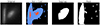Fig. A.1.

Masking routine for VCC 483. From left to right: original r-band postage stamp, hot (red) and cool (blue) runs, final segmentation map and final mask. The red (hot) regions are bright peaks in the images, whereas the blue (cool) regions are extended surfaces with a low surface brightness threshold.

Appendix B: Correcting profiles for inclination effects

The majority of galaxies in the VESTIGE sample have moderate axis ratios between 0.5 and 0.8 – however there are a number of galaxies that are more substantially inclined. Radially averaged profiles of disc galaxies will vary depending on the inclination of the galaxy. The simplest model to correct for inclination effect is to consider the change in projected area for a galaxy with i = 0° to i > 0°. Since the projected area of a disc galaxy with i = 0° is a circle with area A = πa², where a is the semi-major axis then the annulus used to measure surface brightness would have area of A = π(a_out²−a_in²), where a_out and a_in represent the semi major axis (radius) of the outer and inner rings of the annulus, respectively. A galaxy with non-zero inclination will have a projected area of A = πab where b is the semi-minor axis and b = asec(i). Thus, the annuli used to measure the surface brightness will have area A = π(a_outb_out−a_inb_in) = π(a_out²−a_in²)sec(i). The line-of-sight flux measured within the annulus is constant (neglecting inclination effects on extinction), and the surface brightness is measured as μ = −2.5log(F/A) + ZP = m + 2.5log(A) + ZP. Therefore, the difference in surface brightness μ as a function of inclination angle is simply:

$\begin{matrix} μ_{i = 0^{°}} - μ_{i = i^{'}}^{°} & = 2.5 log (\frac{A_{i = 0}^{°}}{A_{i = i^{'}}^{°}}) \\ = 2.5 log (\frac{π (a_{out}^{2} - a_{in}^{2})}{π (a_{out}^{2} - a_{in}^{2}) sec (i)}) \\ = 2.5 log (\frac{1}{sec (i)}) \\ = 2.5 log (\frac{a}{b}) . \end{matrix}$ $\begin{aligned} \mu _{i = 0 ^{\circ }} - \mu _{i=i^{\prime }} ^{\circ }&= 2.5 \log {\left(\frac{A_{i = 0}^{\circ }}{A_{i=i^{\prime }}^{\circ }}\right)}\nonumber \\&= 2.5 \log {\left(\frac{\pi \left(a_{out}^2 - a_{in}^2\right)}{\pi \left(a_{out}^2 - a_{in}^2\right)\sec {(i)}}\right)}\nonumber \\&= 2.5 \log {\left(\frac{1}{\sec {(i)}}\right)}\nonumber \\&= 2.5 \log {\left(\frac{a}{b}\right)}. \end{aligned}$ (B.1)

This simple correction assumes a disc with negligible height and also assumes that internal dust extinction is not a function of inclination. For the purposes of this analysis, we expect that both of these assumptions suffice for b/a > 0.3. After removing these highly inclined objects from our analysis, we find negligible differences in the overall results, so we choose to leave them in our sample.

Appendix C: Examples of peculiar galaxies

C.1. Starburst galaxies with Hα filaments

Starburst galaxies with Hα filaments were not excluded from our sample. The detection of Hα-emitting filaments extending beyond the central starburst give these galaxies R_sSFR/R_norm values close to unity; however, these galaxies do not have an intact SF disc. Fig. C.1 shows VCC 1190 as an example, in the Hα (left) and r-band (right). This galaxy is massive, extremely gas-deficient and yet has R_sSFR/R_norm ∼ 0.9.

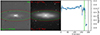Fig. C.1.

Hα NB emission (left), r-band optical emission (centre), and sSFR profile (right) for VCC 1190. In the left and centre postage stamps, the green ellipse outlines R_sSFR while the red ellipse outlines R_norm. On the sSFR plots, we show R_sSFR and its associated uncertainty range as a green vertical line and band, and R_norm and its uncertainty range as a grey vertical line and band.

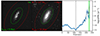Fig. C.2.

Same as Fig. C.1 but for VCC 465. The value shown for R_sSFR is visually a poor representation of the last valid local maximum on the sSFR plot, and drastically overestimates the extent of the Hα emission.

C.2. Galaxies with unphysical R_sSFR

In a small number of cases (18), visual inspection of the sSFR profiles showed features that caused the measured R_sSFR value to be unphysical. Typically this was due to a spike in the sSFR values at large galactocentric radii. This could be due to local background variations or artefacts such as bright star halos that were not entirely masked. Additionally, local variation in the continuum subtraction could bias the Hα flux in low-SB regions to be higher than the true value. All of these galaxies were removed from our sample. We show an example of VCC 497 in Fig. C.2, with the Hα image on the left with an ellipse showing the unphysical R_sSFR and the sSFR profile on the right. Clearly the green ellipse outlining R_sSFR radius extends well beyond the Hα emission.

Appendix D: Galaxy and quenching models

To define the radial profiles of the gas and SFR, we use the sub-kiloparsec Kennicutt-Schmidt law defined by Bigiel et al. (2008) along with the gas density threshold concept used throughout this work. Choosing an example galaxy to have $M_{*} = 10^{9.5} M_{⊙}$ $M_* = 10^{9.5}\,\mathrm{M}_{\odot}$ , our fits to the Σ_*(R_edge)−M_* and R_edge − M_* relations from C22 give a threshold Σ_*(R_edge) = 0.6 M_⊙ pc⁻² and R_edge = 8.1 kpc. Calculating the scale radius of the exponential profile from the critical Σ_* value and the total stellar mass, we land on a scale radius r_s = 1.3 kpc.

From Huang et al. (2012), we have scaling relations for H I and SFR as a function of stellar mass:

$\begin{matrix} log (M_{H} i) = {\begin{matrix} 0.712 log (M_{*}) + 3.117, & log (M_{*}) \leq 9 M_{⊙} \\ 0.276 log (M_{*}) + 7.042, & log (M_{*}) > 9 M_{⊙} \end{matrix}, \end{matrix}$ $\begin{aligned}&\log {(M_{\rm H}{i })} = \left\{ \begin{array}{ll} 0.712\log {(M_{*})} + 3.117,&\log {(M_{*})} \le 9\,\mathrm{M}_{\odot } \\ 0.276\log {(M_{*})} + 7.042,&\log {(M_{*})} > 9\,\mathrm{M}_{\odot } \end{array},\right. \end{aligned}$ (D.1)

$\begin{matrix} log (s S F R) = {\begin{matrix} - 0.149 log (M_{*}) - 8.207, & log (M_{*}) \leq 9.5 M_{⊙} \\ - 0.759 log (M_{*}) - 2.402, & log (M_{*}) > 9.5 M_{⊙} \end{matrix} . \end{matrix}$ $\begin{aligned}&\log {(sSFR)} = \left\{ \begin{array}{ll} -0.149\log {(M_{*})} - 8.207,&\log {(M_{*})} \le 9.5\,\mathrm{M}_{\odot } \\ -0.759\log {(M_{*})} - 2.402,&\log {(M_{*})} > 9.5\,\mathrm{M}_{\odot } \end{array}.\right. \end{aligned}$ (D.2)

For the example galaxy, $M_{*} = 10^{9.5} M_{⊙}$ $M_{*} = 10^{9.5}\,\mathrm{M}_{\odot}$ gives $log (M_{H I}) = 9.7 M_{⊙}$ $\log{(M_{\mathrm{H}\textsc{i}})} = 9.7\,\mathrm{M}_{\odot}$ and SFR = 0.75 M_⊙ yr⁻¹. We can then build a Σ_SFR profile with the same shape as the Σ_* profile if we assume a flat sSFR profile. Following Bigiel et al. (2008), Σ_SFR = 10^−3.1Σ_H₂ (with Σ_SFR in M_⊙ kpc⁻² and Σ_H₂ in M_⊙ pc⁻²) and galaxies have relatively flat H I profiles with a value around 8 M_⊙ pc⁻². This allows us to determine an H₂ profile that also has an edge at 8.1 kpc, and an H I profile that extends beyond the SF disc to 13.5 kpc (assuming the total H I content follows the scaling relations in Huang et al. 2012, our galaxy has $M_{H} I = 10^{9.7} M_{⊙}$ $M_{\mathrm{H}}{\textsc{i}} = 10^{9.7}\,\mathrm{M}_{\odot}$ ). The initial gas and SFR density profiles for the galaxy are shown in Fig. D.1. Since the edge of the galaxy occurs at 8.1 kpc and beyond this point there is only H I gas, the total gas density threshold for star formation is determined by this value of H I, which is 8 M_⊙ pc⁻².

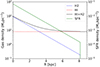Fig. D.1.

Initial SFR (green), H I (red), H₂ (blue) and total gas (black) density profiles for a $10^{9.5} M_{⊙}$ $10^{9.5}\,\mathrm{M}_{\odot}$ galaxy.

We assume that there is no radial dependence of the H I to H₂ conversion, and that the global H I content just drops by whatever amount necessary to replenish the H₂ at each timestep. As such, the H I profile drops but remains constant at all radii. In Fig. D.2, we show the gas and SFR density profiles in the first and second rows, respectively. Each column shows a different timestep (2, 5 and 8 Gyr after infall). On the SFR density plots, we show the R_sSFR determined by where the total gas density falls below the threshold value of 8 M_⊙ pc⁻². In the bottom row, we show the evolution of the global SFR, gas deficiency and R_sSFR. We see that in this model, truncations occur early as the H I begins to deplete; however it takes several gigayears for the global SFR to drop significantly; by this time, the galaxy is completely anaemic in terms of its H I gas content.

Our RPS model assumes a galaxy falling into the cluster radially and face-on, such that the direction of the ram-pressure force is orthogonal to the plane of the disc. The efficiency of RPS can vary moderately as a function of inclination angle (e.g. Roediger & Brüggen 2006; Steinhauser et al. 2016). The restoring force holding the gas to the galactic disc is given by

$\begin{matrix} f = [g_{*} (r) + g_{H i} (r) + g_{H_{2}} (r) + g_{DM} (r)] Σ_{H i} (r), \end{matrix}$ $\begin{aligned} f = \left[g_{*}(\mathrm{r}) + g_{\mathrm{H}i }(r) + g_{\mathrm{{H}}_{2}}(r) + g_{\rm DM}(r)\right] \,\Sigma _{\mathrm{H}i }(r), \end{aligned}$ (D.3)

where g_*(r), $g_{H I} (r)$ $g_{\mathrm{H}\textsc{i}}(r)$ , g_H₂(r) and g_DM(r) are the contributions to the gravitational acceleration from the different galactic components (stars, H I, H₂ and dark matter), and $Σ_{H I} (r)$ $\Sigma_{\mathrm{H}\textsc{i}}(r)$ is the surface density of H I gas. Since our stellar component is simply an exponential disc, it follows that

$\begin{matrix} g_{*} (r) = 2 π G Σ_{*} (r) = 2 π G Σ_{0, *} e^{- r / r_{s}}, \end{matrix}$ $\begin{aligned} g_*(r) = 2\pi G \Sigma _*(r) = 2\pi G \Sigma _{0,*} e^\mathrm{-r/r_s}, \end{aligned}$ (D.4)

where Σ_0, * is the central stellar mass surface density and r_s is the scale radius. Our H₂ profile is also an exponential so it will take the same form. Our H I profile is flat and as such $Σ_{H I} (r) = Σ_{0, HI}$ $\Sigma_{\mathrm{H}\textsc{i}}(r) = \Sigma_{\mathrm{0,HI}}$ . For the dark matter halo, we deviate from Roberts et al. (2019) only in that we use a Navarro-Frenk-White (NFW; Navarro et al. 1996) profile instead of a Hernquist profile (Hernquist 1990), with

$\begin{matrix} Φ (r, z) = \frac{4 π G ρ_{0} a^{3}}{\sqrt{r^{2} + z^{2}}} ln (1 + \frac{\sqrt{r^{2} + z^{2}}}{a}), \end{matrix}$ $\begin{aligned} \Phi (r, \, z) = \frac{4\pi G \rho _0 a^3}{\sqrt{r^2 + z^2}} \ln {\left(1 + \frac{\sqrt{r^2 + z^2}}{a}\right)}, \end{aligned}$ (D.5)

where we determine the halo mass, M_h, from the stellar-to-halo mass relation of Girelli et al. (2020), which allows the determination of R₂₀₀. The scale radius, a = R₂₀₀/c, where c is the concentration determined from the concentration-halo mass relation from Diemer & Kravtsov (2015). ρ₀ is the central density of the NFW profile which can be be determined from M_h, R₂₀₀ and a. We calculate the gravitational acceleration of the dark matter profile by taking the maximum of the derivative along the z axis, where z is the direction perpendicular to the disc:

$\begin{matrix} \begin{matrix} g_{DM} (r) & = max_{z} \frac{\partial Φ (r, z)}{\partial z} \\ = max_{z} 4 π G ρ_{0} a^{3} z [\frac{ln (a + \sqrt{r^{2} + z^{2}}) - ln (a)}{{(r^{2} + z^{2})}^{3 / 2}} \\ - \frac{1}{(r^{2} + z^{2}) (a + \sqrt{r^{2} + z^{2}})}] . \end{matrix} \end{matrix}$ $\begin{aligned} \begin{aligned} g_{\rm DM}(r)&= \max _{\rm z} \frac{\partial \Phi (r,\,z)}{\partial z} \\&= \max _{\rm z} 4 \pi G \rho _{0} a^{3} z \left[\frac{\ln {\left(a + \sqrt{r^2 + z^2}\right)} - \ln (a)}{\left(r^2 + z^2\right)^{3/2}}\right. \\&\left. -\frac{1}{\left(r^2 + z^2\right) \left(a + \sqrt{r^2 + z^2}\right)}\right]. \end{aligned} \end{aligned}$ (D.6)

To determine the ram-pressure at a given point in phase space, we use the beta profile fit from Schindler et al. (1999), with r_c = 12.9 kpc and β = 0.47, and determine the central ICM density from Simionescu et al. (2017) to be n₀ = 2.33 × 10⁻² cm⁻³. We then can determine the ICM mass density based on this relation from Boselli et al. (2022):

$\begin{matrix} ρ_{ICM} (r) = 1.92 μ n_{e} (r) m_{p} = 1.15 n_{e} (r) m_{p}, \end{matrix}$ $\begin{aligned} \rho _{\rm ICM}(r) = 1.92 \, \mu \, n_{\rm e}(r) \, m_{\rm p} = 1.15 \, n_{\rm e}(r) \, m_{\rm p}, \end{aligned}$ (D.7)

where μ = 0.6.

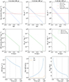Fig. D.2.

Top: Gas density profiles at three timesteps for starvation model. Initial profiles for H I and H₂ are shown in red and blue, respectively while evolved profiles are shown in pink and light blue, respectively. Evolved total gas density profile is shown in black. Middle: SFR density profiles at three timesteps, where the initial profile is shown in green and the evolved profile in light green. The grey vertical line shows R_sSFR. Bottom: Time evolution of global SFR, gas deficiency and R_sSFR.

Appendix E: Additional radial profile plots

We show in Fig. E.1 the equivalent of Fig. 1 for eight galaxies spanning a range of stellar masses.

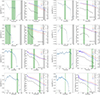Fig. E.1.

Same as Fig. 1 but for all galaxies shown in Fig. F.1. From top to bottom and left to right: VCC 304, VCC 2037, VCC 865 (NGC 4396), VCC 157 (NGC 4208), VCC 1605, VCC 565, VCC 1868 (NGC 4607) and VCC 596 (NGC 4321).

Appendix F: Additional postage stamps

In Fig. F.1, we show postage stamps alongside radial sSFR profiles (same as Fig. 3) for eight galaxies spanning a range of stellar masses.

Fig. F.1.

Same as Fig. 3 for VCC 304, VCC 2037, VCC 865 (NGC 4396), and VCC 157 (NGC 4208).

Fig. F.2.

(Cont.). Same as Fig. 3 for VCC 1605, VCC 565, VCC 1868 (NGC 4607) and VCC 596 (NGC 4321).

All Tables

Table 1.

Properties of Virgo cluster substructures (taken from Boselli et al. 2023b).

In the text

Table A.1.

PHOTUTILS parameters used in object masking routine

In the text

All Figures

Fig. 1.

Radial profiles for VCC 865 (NGC 4396). Left: sSFR profile (blue data points) with a smoothed profile shown as a black curve. The next five upper limits (where no Hα is detected but stellar mass is) are shown as blue arrows, connected by a dot-dashed line. Right: Surface brightness profiles for Hα NB (black) and r-band emission (red), along with the Σ_* profile (blue). The dashed black profile shows the detection limit for the Hα profile. In both panels, the green vertical line shows the median SF disc edge, R_sSFR, and the shaded green band the uncertainty range based on the 16^th and 84^th percentiles computed using a Monte Carlo simulation with 1000 iterations. The vertical black line shows the expected edge, R_norm, of the galaxy and the shaded grey band uncertainty range based on the 16^th and 84^th percentiles of the Monte Carlo simulation.

In the text

	Fig. 2. Recovered total stellar masses obtained by numerically integrating Σ_* profiles up to R_norm compared to stellar masses obtained by Boselli et al. (2023a) through SED fitting.
In the text

Fig. 3.

Continuum-subtracted Hα emission (left), r-band optical emission (centre), and sSFR profile (right) for VCC 865 (NGC 4396). In the left and centre postage stamps, the green ellipse outlines R_sSFR while the red ellipse outlines R_norm. On the sSFR plots (right), we show R_sSFR and its associated uncertainty range as a green vertical line and band, and R_norm and its uncertainty range as a grey vertical line and band. Also included are the upper limits (down arrows) in the next five radial bins in which Hα is not detected (but stellar mass is); this represents the upper limit to the sSFR based on the Hα detection limits.

In the text

	Fig. 4. Size-stellar mass relations. Left: Size-stellar mass relation for galaxies with identified R_norm. We fit a linear relation to the data and show that a slope of m = 0.34 ± 0.01 is measured, consistent with C22. The shaded grey region shows the 1σ scatter in the linear relation. Right: Size-stellar mass relation using R_sSFR, showing the linear fit to the R_norm-mass relation.
In the text

Fig. 5.

R_sSFR/R_norm as a function of stellar mass. The two shaded grey regions show limits on the measurements of R_sSFR/R_norm. We have excluded any galaxies where the sSFR profile spans fewer than three data points, so the dashed black line has R_sSFR = 6.545″. In principle, any sSFR profile with more than three data points could still have a truncation at the first data point, so the dash-dotted line has R_sSFR = 2.805″. In both cases, R_norm is determined from the size mass relation in Fig. 4 at a distance of 16.5 Mpc.

In the text

Fig. 6.

R_sSFR/R_norm against star formation indicators. Left: R_sSFR/R_norm as a function of H I-deficiency, with galaxies located on or above the SFMS shown in red and galaxies below the SFMS shown in blue. The range of H I-normal galaxies is shaded. Right: R_sSFR/R_norm as a function of distance from the SFMS, with H I-normal galaxies shown in red and H I-deficient galaxies shown in blue. The SFMS is shown as a shaded region.

In the text

Fig. 7.

Right ascension and declination footprint of VESTIGE galaxies with measured values of R_sSFR/R_norm. Overplotted are the seven identified regions associated with the Virgo cluster: Clusters A, B and C, the W and W′ clouds, the M cloud and the Low-Velocity cloud, with the radii noted in Table 1. Data points are sized proportionally to the stellar mass of the galaxy, and coloured based on the value of R_sSFR/R_norm.

In the text

	Fig. 8. Box-and-whisker plot showing the median and first and third quartiles of the distributions of R_sSFR/R_norm in the entire sample and four groupings of Virgo cluster substructures. ‘Other groups’ covers the M and low-velocity clouds as well as Cluster C.
In the text

	Fig. 9. PPS diagram of VESTIGE galaxies with VESTIGE Hα detection fractions computed using the ratio of 2D Gaussian KDEs of the VESTIGE and NGVS distributions. Data points are sized proportionally to the stellar mass of the galaxy, and coloured based on the value of R_sSFR/R_norm. While the detection fractions show the expected structure, truncated discs exist across the cluster environment.
In the text

Fig. 10.

PPS diagram showing the region within the escape velocity of the cluster as the region between the two dashed black lines. The escape velocity is determined based on the NFW profile of Simionescu et al. (2017). The green, yellow, and red lines show the contours where a M_* = 10^9.5 M_⊙ galaxy could have its gas removed by RPS from 0.01, 0.5, and 1 R_norm, respectively, assuming isotropic orbits. Data points are sized proportionally to the stellar mass of the galaxy, and coloured based on the value of R_sSFR/R_norm. The background greyscale shows the phase-space number density of galaxies with 0.3 < R_sSFR/R_norm < 0.7 determined using a 2D Gaussian KDE.

In the text

Fig. 11.

Evolution of total gas density (Σ_HI + Σ_H2) over 8 Gyr for a $M_{*} = 10^{9.5} M_{⊙}$ $M_* = 10^{9.5}\,\mathrm{M}_{\odot}$ galaxy undergoing simple starvation. The threshold gas density for star formation (explained in Appendix D) is shown as a dashed red line. By the t = 8 Gyr curve, all H I gas has been consumed and as such the H₂ is not being replenished, causing the total gas density to decrease at all radii.

In the text

	Fig. 12. Evolution through time of R_sSFR (top) and H I-deficiency (bottom), for a M_* = 10^9.5 M_⊙ galaxy undergoing a simple starvation model (blue curves) and a galaxy falling into Virgo radially and experiencing RPS along with starvation (red curves). The horizontal dashed black line at H I-def = 0.4 represents the point above which a galaxy is considered H I-deficient.
In the text

	Fig. A.1. Masking routine for VCC 483. From left to right: original r-band postage stamp, hot (red) and cool (blue) runs, final segmentation map and final mask. The red (hot) regions are bright peaks in the images, whereas the blue (cool) regions are extended surfaces with a low surface brightness threshold.
In the text

Fig. C.1.

Hα NB emission (left), r-band optical emission (centre), and sSFR profile (right) for VCC 1190. In the left and centre postage stamps, the green ellipse outlines R_sSFR while the red ellipse outlines R_norm. On the sSFR plots, we show R_sSFR and its associated uncertainty range as a green vertical line and band, and R_norm and its uncertainty range as a grey vertical line and band.

In the text

	Fig. C.2. Same as Fig. C.1 but for VCC 465. The value shown for R_sSFR is visually a poor representation of the last valid local maximum on the sSFR plot, and drastically overestimates the extent of the Hα emission.
In the text

	Fig. D.1. Initial SFR (green), H I (red), H₂ (blue) and total gas (black) density profiles for a $10^{9.5} M_{⊙}$ $10^{9.5}\,\mathrm{M}_{\odot}$ galaxy.
In the text

Fig. D.2.

Top: Gas density profiles at three timesteps for starvation model. Initial profiles for H I and H₂ are shown in red and blue, respectively while evolved profiles are shown in pink and light blue, respectively. Evolved total gas density profile is shown in black. Middle: SFR density profiles at three timesteps, where the initial profile is shown in green and the evolved profile in light green. The grey vertical line shows R_sSFR. Bottom: Time evolution of global SFR, gas deficiency and R_sSFR.

In the text

	Fig. E.1. Same as Fig. 1 but for all galaxies shown in Fig. F.1. From top to bottom and left to right: VCC 304, VCC 2037, VCC 865 (NGC 4396), VCC 157 (NGC 4208), VCC 1605, VCC 565, VCC 1868 (NGC 4607) and VCC 596 (NGC 4321).
In the text

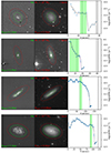	Fig. F.1. Same as Fig. 3 for VCC 304, VCC 2037, VCC 865 (NGC 4396), and VCC 157 (NGC 4208).
In the text

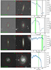	Fig. F.2. (Cont.). Same as Fig. 3 for VCC 1605, VCC 565, VCC 1868 (NGC 4607) and VCC 596 (NGC 4321).
In the text

Current usage metrics show cumulative count of Article Views (full-text article views including HTML views, PDF and ePub downloads, according to the available data) and Abstracts Views on Vision4Press platform.

Data correspond to usage on the plateform after 2015. The current usage metrics is available 48-96 hours after online publication and is updated daily on week days.

Initial download of the metrics may take a while.

[1] Alberts, S., Adams, J., Gregg, B., et al. 2022, ApJ, 927, 235 [NASA ADS] [CrossRef] [Google Scholar]

[2] Astropy Collaboration (Robitaille, T. P., et al.) 2013, A&A, 558, A33 [NASA ADS] [CrossRef] [EDP Sciences] [Google Scholar]

[3] Astropy Collaboration (Price-Whelan, A. M., et al.) 2018, AJ, 156, 123 [Google Scholar]

[4] Astropy Collaboration (Price-Whelan, A. M., et al.) 2022, ApJ, 935, 167 [NASA ADS] [CrossRef] [Google Scholar]

[5] Bahé, Y. M., McCarthy, I. G., Balogh, M. L., & Font, A. S. 2013, MNRAS, 430, 3017 [Google Scholar]

[6] Baldry, I. K., Balogh, M. L., Bower, R. G., et al. 2006, MNRAS, 373, 469 [Google Scholar]

[7] Balogh, M. L., Morris, S. L., Yee, H. K. C., Carlberg, R. G., & Ellingson, E. 1997, ApJ, 488, L75 [NASA ADS] [CrossRef] [Google Scholar]

[8] Balogh, M. L., Schade, D., Morris, S. L., et al. 1998, ApJ, 504, L75 [NASA ADS] [CrossRef] [Google Scholar]

[9] Balogh, M. L., Navarro, J. F., & Morris, S. L. 2000, ApJ, 540, 113 [Google Scholar]

[10] Balogh, M. L., McGee, S. L., Mok, A., et al. 2016, MNRAS, 456, 4364 [NASA ADS] [CrossRef] [Google Scholar]

[11] Barnes, J. E. 2004, MNRAS, 350, 798 [NASA ADS] [CrossRef] [Google Scholar]

[12] Bekki, K. 2009, MNRAS, 399, 2221 [Google Scholar]

[13] Belfiore, F., Maiolino, R., Bundy, K., et al. 2018, MNRAS, 477, 3014 [Google Scholar]

[14] Bigiel, F., Leroy, A., Walter, F., et al. 2008, AJ, 136, 2846 [NASA ADS] [CrossRef] [Google Scholar]

[15] Binggeli, B., Sandage, A., & Tammann, G. A. 1985, AJ, 90, 1681 [Google Scholar]

[16] Binggeli, B., Tammann, G. A., & Sandage, A. 1987, AJ, 94, 251 [Google Scholar]

[17] Boquien, M., Burgarella, D., Roehlly, Y., et al. 2019, A&A, 622, A103 [NASA ADS] [CrossRef] [EDP Sciences] [Google Scholar]

[18] Boselli, A., & Gavazzi, G. 2006, PASP, 118, 517 [Google Scholar]

[19] Boselli, A., & Gavazzi, G. 2014, A&ARv, 22, 74 [Google Scholar]

[20] Boselli, A., Boissier, S., Cortese, L., et al. 2006, ApJ, 651, 811 [Google Scholar]

[21] Boselli, A., Boissier, S., Heinis, S., et al. 2011, A&A, 528, A107 [NASA ADS] [CrossRef] [EDP Sciences] [Google Scholar]

[22] Boselli, A., Cortese, L., Boquien, M., et al. 2014a, A&A, 564, A67 [NASA ADS] [CrossRef] [EDP Sciences] [Google Scholar]

[23] Boselli, A., Voyer, E., Boissier, S., et al. 2014b, A&A, 570, A69 [NASA ADS] [CrossRef] [EDP Sciences] [Google Scholar]

[24] Boselli, A., Cuillandre, J. C., Fossati, M., et al. 2016, A&A, 587, A68 [NASA ADS] [CrossRef] [EDP Sciences] [Google Scholar]

[25] Boselli, A., Fossati, M., Ferrarese, L., et al. 2018a, A&A, 614, A56 [NASA ADS] [CrossRef] [EDP Sciences] [Google Scholar]

[26] Boselli, A., Fossati, M., Consolandi, G., et al. 2018b, A&A, 620, A164 [NASA ADS] [CrossRef] [EDP Sciences] [Google Scholar]

[27] Boselli, A., Fossati, M., Longobardi, A., et al. 2019, A&A, 623, A52 [NASA ADS] [CrossRef] [EDP Sciences] [Google Scholar]

[28] Boselli, A., Fossati, M., Longobardi, A., et al. 2020, A&A, 634, L1 [NASA ADS] [CrossRef] [EDP Sciences] [Google Scholar]

[29] Boselli, A., Lupi, A., Epinat, B., et al. 2021, A&A, 646, A139 [NASA ADS] [CrossRef] [EDP Sciences] [Google Scholar]

[30] Boselli, A., Fossati, M., & Sun, M. 2022, A&ARv, 30, 3 [NASA ADS] [CrossRef] [Google Scholar]

[31] Boselli, A., Fossati, M., Roediger, J., et al. 2023a, A&A, 669, A73 [NASA ADS] [CrossRef] [EDP Sciences] [Google Scholar]

[32] Boselli, A., Fossati, M., Côté, P., et al. 2023b, A&A, 675, A123 [NASA ADS] [CrossRef] [EDP Sciences] [Google Scholar]

[33] Boselli, A., Serra, P., de Gasperin, F., et al. 2023c, A&A, 676, A92 [NASA ADS] [CrossRef] [EDP Sciences] [Google Scholar]

[34] Bradley, L., Sipőcz, B., Robitaille, T., et al. 2021, https://doi.org/10.5281/zenodo.4453725 [Google Scholar]

[35] Brown, T., Roberts, I. D., Thorp, M., et al. 2023, ApJ, 956, 37 [NASA ADS] [CrossRef] [Google Scholar]

[36] Bruzual, G., & Charlot, S. 2003, MNRAS, 344, 1000 [NASA ADS] [CrossRef] [Google Scholar]

[37] Bundy, K., Bershady, M. A., Law, D. R., et al. 2015, ApJ, 798, 7 [Google Scholar]

[38] Butcher, H., & Oemler, A. 1984, ApJ, 285, 426 [NASA ADS] [CrossRef] [Google Scholar]

[39] Calzetti, D., Wu, S. Y., Hong, S., et al. 2010, ApJ, 714, 1256 [NASA ADS] [CrossRef] [Google Scholar]

[40] Cattorini, F., Gavazzi, G., Boselli, A., & Fossati, M. 2023, A&A, 671, A118 [NASA ADS] [CrossRef] [EDP Sciences] [Google Scholar]

[41] Cayatte, V., van Gorkom, J. H., Balkowski, C., & Kotanyi, C. 1990, AJ, 100, 604 [NASA ADS] [CrossRef] [Google Scholar]

[42] Cayatte, V., Kotanyi, C., Balkowski, C., & van Gorkom, J. H. 1994, AJ, 107, 1003 [Google Scholar]

[43] Chabrier, G. 2003, PASP, 115, 763 [Google Scholar]

[44] Chamaraux, P., Balkowski, C., & Gerard, E. 1980, A&A, 83, 38 [NASA ADS] [Google Scholar]

[45] Chamba, N., Trujillo, I., & Knapen, J. H. 2020, A&A, 633, L3 [NASA ADS] [CrossRef] [EDP Sciences] [Google Scholar]

[46] Chamba, N., Trujillo, I., & Knapen, J. H. 2022, A&A, 667, A87 [NASA ADS] [CrossRef] [EDP Sciences] [Google Scholar]

[47] Chung, A., van Gorkom, J. H., Kenney, J. D. P., & Vollmer, B. 2007, ApJ, 659, L115 [Google Scholar]

[48] Chung, A., van Gorkom, J. H., Kenney, J. D. P., Crowl, H., & Vollmer, B. 2009, AJ, 138, 1741 [Google Scholar]

[49] Chyży, K. T., Ehle, M., & Beck, R. 2007, A&A, 474, 415 [NASA ADS] [CrossRef] [EDP Sciences] [Google Scholar]

[50] Conroy, C., Gunn, J. E., & White, M. 2009, ApJ, 699, 486 [Google Scholar]

[51] Cooke, E. A., Hatch, N. A., Stern, D., et al. 2016, ApJ, 816, 83 [NASA ADS] [CrossRef] [Google Scholar]

[52] Cortese, L., Catinella, B., Boissier, S., Boselli, A., & Heinis, S. 2011, MNRAS, 415, 1797 [Google Scholar]

[53] Cortese, L., Boissier, S., Boselli, A., et al. 2012, A&A, 544, A101 [NASA ADS] [CrossRef] [EDP Sciences] [Google Scholar]

[54] Cortese, L., Catinella, B., & Smith, R. 2021, PASA, 38, e035 [NASA ADS] [CrossRef] [Google Scholar]

[55] Crowl, H. H., Kenney, J. D. P., van Gorkom, J. H., & Vollmer, B. 2005, AJ, 130, 65 [Google Scholar]

[56] de Vaucouleurs, G. 1948, Ann. Astrophys., 11, 247 [Google Scholar]

[57] Diemer, B., & Kravtsov, A. V. 2015, ApJ, 799, 108 [Google Scholar]

[58] Dressler, A. 1980, ApJ, 236, 351 [Google Scholar]

[59] Dressler, A., Oemler, A., Couch, W. J., et al. 1997, ApJ, 490, 577 [NASA ADS] [CrossRef] [Google Scholar]

[60] Ebeling, H., Stephenson, L. N., & Edge, A. C. 2014, ApJ, 781, L40 [Google Scholar]

[61] Erwin, P., Pohlen, M., & Beckman, J. E. 2008, AJ, 135, 20 [Google Scholar]

[62] Faber, S. M., Willmer, C. N. A., Wolf, C., et al. 2007, ApJ, 665, 265 [Google Scholar]

[63] Ferrarese, L., Côté, P., Cuillandre, J.-C., et al. 2012, ApJS, 200, 4 [Google Scholar]

[64] Ferrarese, L., Côté, P., MacArthur, L. A., et al. 2020, ApJ, 890, 128 [Google Scholar]

[65] Finn, R. A., Desai, V., Rudnick, G., et al. 2018, ApJ, 862, 149 [NASA ADS] [CrossRef] [Google Scholar]

[66] Fossati, M., Gavazzi, G., Savorgnan, G., et al. 2013, A&A, 553, A91 [NASA ADS] [CrossRef] [EDP Sciences] [Google Scholar]

[67] Fossati, M., Mendel, J. T., Boselli, A., et al. 2018, A&A, 614, A57 [NASA ADS] [CrossRef] [EDP Sciences] [Google Scholar]

[68] Freeman, K. C. 1970, ApJ, 160, 811 [Google Scholar]

[69] Galametz, A., Grazian, A., Fontana, A., et al. 2013, ApJS, 206, 10 [Google Scholar]

[70] Gavazzi, G., Boselli, A., Scodeggio, M., Pierini, D., & Belsole, E. 1999, MNRAS, 304, 595 [Google Scholar]

[71] Gavazzi, G., Boselli, A., Mayer, L., et al. 2001, ApJ, 563, L23 [Google Scholar]

[72] Gavazzi, G., Boselli, A., Donati, A., Franzetti, P., & Scodeggio, M. 2003, A&A, 400, 451 [NASA ADS] [CrossRef] [EDP Sciences] [Google Scholar]

[73] Gavazzi, G., Boselli, A., van Driel, W., & O’Neil, K. 2005, A&A, 429, 439 [NASA ADS] [CrossRef] [EDP Sciences] [Google Scholar]

[74] Gavazzi, G., Boselli, A., Cortese, L., et al. 2006, A&A, 446, 839 [NASA ADS] [CrossRef] [EDP Sciences] [Google Scholar]

[75] Gavazzi, G., Savorgnan, G., Fossati, M., et al. 2013a, A&A, 553, A90 [NASA ADS] [CrossRef] [EDP Sciences] [Google Scholar]

[76] Gavazzi, G., Fumagalli, M., Fossati, M., et al. 2013b, A&A, 553, A89 [NASA ADS] [CrossRef] [EDP Sciences] [Google Scholar]

[77] Giovanelli, R., & Haynes, M. P. 1983, AJ, 88, 881 [Google Scholar]

[78] Giovanelli, R., & Haynes, M. P. 1985, ApJ, 292, 404 [CrossRef] [Google Scholar]

[79] Giovanelli, R., Haynes, M. P., Kent, B. R., et al. 2005, AJ, 130, 2598 [Google Scholar]

[80] Girelli, G., Pozzetti, L., Bolzonella, M., et al. 2020, A&A, 634, A135 [NASA ADS] [CrossRef] [EDP Sciences] [Google Scholar]

[81] Goddard, D., Thomas, D., Maraston, C., et al. 2017, MNRAS, 465, 688 [Google Scholar]

[82] Gómez, P. L., Nichol, R. C., Miller, C. J., et al. 2003, ApJ, 584, 210 [Google Scholar]

[83] González Delgado, R. M., García-Benito, R., Pérez, E., et al. 2015, A&A, 581, A103 [Google Scholar]

[84] Goto, T., Yamauchi, C., Fujita, Y., et al. 2003, MNRAS, 346, 601 [NASA ADS] [CrossRef] [Google Scholar]

[85] Greener, M. J., Aragón-Salamanca, A., Merrifield, M. R., et al. 2020, MNRAS, 495, 2305 [CrossRef] [Google Scholar]

[86] Gunn, J. E., & Gott, J. R. 1972, ApJ, 176, 1 [NASA ADS] [CrossRef] [Google Scholar]

[87] Gwyn, S. D. J. 2008, PASP, 120, 212 [Google Scholar]

[88] Haynes, M. P., Giovanelli, R., Kent, B. R., et al. 2018, ApJ, 861, 49 [Google Scholar]

[89] Hernquist, L. 1990, ApJ, 356, 359 [Google Scholar]

[90] Herrmann, K. A., Hunter, D. A., & Elmegreen, B. G. 2013, AJ, 146, 104 [NASA ADS] [CrossRef] [Google Scholar]

[91] Herrmann, K. A., Hunter, D. A., & Elmegreen, B. G. 2016, AJ, 151, 145 [NASA ADS] [CrossRef] [Google Scholar]

[92] Huang, S., Haynes, M. P., Giovanelli, R., & Brinchmann, J. 2012, ApJ, 756, 113 [Google Scholar]

[93] Huchra, J., Davis, M., Latham, D., & Tonry, J. 1983, ApJS, 52, 89 [NASA ADS] [CrossRef] [Google Scholar]

[94] Hunter, J. D. 2007, Comput. Sci. Eng., 9, 90 [NASA ADS] [CrossRef] [Google Scholar]

[95] Hunter, D. A., & Elmegreen, B. G. 2006, ApJS, 162, 49 [NASA ADS] [CrossRef] [Google Scholar]

[96] Jedrzejewski, R. I. 1987, MNRAS, 226, 747 [Google Scholar]

[97] Johnson, B. D., Leja, J., Conroy, C., & Speagle, J. S. 2021, ApJS, 254, 22 [NASA ADS] [CrossRef] [Google Scholar]

[98] Junais, Boissier, S., Boselli, A., et al. 2022, A&A, 667, A76 [NASA ADS] [CrossRef] [EDP Sciences] [Google Scholar]

[99] Kantharia, N. G., Rao, A. P., & Sirothia, S. K. 2008, MNRAS, 383, 173 [Google Scholar]

[100] Kauffmann, G., White, S. D. M., Heckman, T. M., et al. 2004, MNRAS, 353, 713 [Google Scholar]

[101] Kawata, D., & Mulchaey, J. S. 2008, ApJ, 672, L103 [NASA ADS] [CrossRef] [Google Scholar]

[102] Kawinwanichakij, L., Papovich, C., Quadri, R. F., et al. 2017, ApJ, 847, 134 [NASA ADS] [CrossRef] [Google Scholar]

[103] Kelkar, K., Dwarakanath, K. S., Poggianti, B. M., et al. 2020, MNRAS, 496, 442 [NASA ADS] [CrossRef] [Google Scholar]

[104] Kenney, J. D. P., van Gorkom, J. H., & Vollmer, B. 2004, AJ, 127, 3361 [Google Scholar]

[105] Kennicutt, R. C. 1989, ApJ, 344, 685 [Google Scholar]

[106] Kennicutt, R. C. 1998, ARA&A, 36, 189 [NASA ADS] [CrossRef] [Google Scholar]

[107] Kim, S., Rey, S.-C., Jerjen, H., et al. 2014, ApJS, 215, 22 [Google Scholar]

[108] Koopmann, R. A., & Kenney, J. D. P. 2004, ApJ, 613, 866 [Google Scholar]

[109] Koopmann, R. A., Haynes, M. P., & Catinella, B. 2006, AJ, 131, 716 [NASA ADS] [CrossRef] [Google Scholar]

[110] Larson, R. B., Tinsley, B. M., & Caldwell, C. N. 1980, ApJ, 237, 692 [Google Scholar]

[111] Lewis, I., Balogh, M., De Propris, R., et al. 2002, MNRAS, 334, 673 [NASA ADS] [CrossRef] [Google Scholar]

[112] Lim, S., Côté, P., Peng, E. W., et al. 2020, ApJ, 899, 69 [CrossRef] [Google Scholar]

[113] Lin, L., Jian, H.-Y., Foucaud, S., et al. 2014, ApJ, 782, 33 [NASA ADS] [CrossRef] [Google Scholar]

[114] Lotz, M., Dolag, K., Remus, R.-S., & Burkert, A. 2021, MNRAS, 506, 4516 [NASA ADS] [CrossRef] [Google Scholar]

[115] Chamba, N., Hayes, M. J., & LSST Dark Energy Science Collaboration 2024, A&A, 689, A28 [NASA ADS] [CrossRef] [EDP Sciences] [Google Scholar]

[116] McCarthy, I. G., Frenk, C. S., Font, A. S., et al. 2008, MNRAS, 383, 593 [NASA ADS] [CrossRef] [Google Scholar]

[117] McKinney, W. 2010, Proceedings of the 9th Python in Science Conference, Austin, 445, 51 [Google Scholar]

[118] McLaughlin, D. E. 1999, ApJ, 512, L9 [Google Scholar]

[119] Mei, S., Blakeslee, J. P., Côté, P., et al. 2007, ApJ, 655, 144 [Google Scholar]

[120] Minchin, R. F., Taylor, R., Köppen, J., et al. 2019, AJ, 158, 121 [NASA ADS] [CrossRef] [Google Scholar]

[121] Moore, B., Katz, N., Lake, G., Dressler, A., & Oemler, A. 1996, Nature, 379, 613 [Google Scholar]

[122] Moore, B., Lake, G., & Katz, N. 1998, ApJ, 495, 139 [Google Scholar]

[123] Moss, C., & Whittle, M. 1993, ApJ, 407, L17 [NASA ADS] [CrossRef] [Google Scholar]

[124] Moss, C., & Whittle, M. 2000, MNRAS, 317, 667 [NASA ADS] [CrossRef] [Google Scholar]

[125] Muzzin, A., Marchesini, D., Stefanon, M., et al. 2013, ApJ, 777, 18 [NASA ADS] [CrossRef] [Google Scholar]

[126] Navarro, J. F., Frenk, C. S., & White, S. D. M. 1996, ApJ, 462, 563 [Google Scholar]

[127] Oemler, A. 1974, ApJ, 194, 1 [Google Scholar]

[128] Peng, Y.-J., Lilly, S. J., Kovač, K., et al. 2010, ApJ, 721, 193 [Google Scholar]

[129] Pérez, F., & Granger, B. E. 2007, Comput. Sci. Eng., 9, 21 [Google Scholar]

[130] Poggianti, B. M., Fasano, G., Omizzolo, A., et al. 2016, AJ, 151, 78 [Google Scholar]

[131] Poggianti, B. M., Moretti, A., Gullieuszik, M., et al. 2017, ApJ, 844, 48 [Google Scholar]

[132] Pohlen, M., & Trujillo, I. 2006, A&A, 454, 759 [NASA ADS] [CrossRef] [EDP Sciences] [Google Scholar]

[133] Quadri, R. F., Williams, R. J., Franx, M., & Hildebrandt, H. 2012, ApJ, 744, 88 [NASA ADS] [CrossRef] [Google Scholar]

[134] Reback, J., McKinney, W., Van den Bossche, J., et al. 2020, https://doi.org/10.5281/zenodo.3993412 [Google Scholar]

[135] Rhee, J., Smith, R., Choi, H., et al. 2017, ApJ, 843, 128 [Google Scholar]

[136] Rich, J. A., Kewley, L. J., & Dopita, M. A. 2011, ApJ, 734, 87 [NASA ADS] [CrossRef] [Google Scholar]

[137] Roberts, I. D., Parker, L. C., Brown, T., et al. 2019, ApJ, 873, 42 [CrossRef] [Google Scholar]

[138] Roberts, I. D., van Weeren, R. J., McGee, S. L., et al. 2021, A&A, 652, A153 [NASA ADS] [CrossRef] [EDP Sciences] [Google Scholar]

[139] Roediger, E., & Brüggen, M. 2006, MNRAS, 369, 567 [NASA ADS] [CrossRef] [Google Scholar]

[140] Roediger, J. C., & Courteau, S. 2015, MNRAS, 452, 3209 [NASA ADS] [CrossRef] [Google Scholar]

[141] Saitoh, T. R., Daisaka, H., Kokubo, E., et al. 2009, PASJ, 61, 481 [NASA ADS] [Google Scholar]

[142] Sánchez, S. F., Kennicutt, R. C., Gil de Paz, A., et al. 2012, A&A, 538, A8 [Google Scholar]

[143] Sazonova, E., Alatalo, K., Lotz, J., et al. 2020, ApJ, 899, 85 [Google Scholar]

[144] Sazonova, E., Alatalo, K., Rowlands, K., et al. 2021, ApJ, 919, 134 [NASA ADS] [CrossRef] [Google Scholar]

[145] Schindler, S., Binggeli, B., & Böhringer, H. 1999, A&A, 343, 420 [Google Scholar]

[146] Serra, P., Maccagni, F. M., Kleiner, D., et al. 2023, A&A, 673, A146 [NASA ADS] [CrossRef] [EDP Sciences] [Google Scholar]

[147] Sérsic, J. L. 1963, Boletin de la Asociacion Argentina de Astronomia La Plata Argentina, 6, 41 [Google Scholar]

[148] Simionescu, A., Werner, N., Mantz, A., Allen, S. W., & Urban, O. 2017, MNRAS, 469, 1476 [Google Scholar]

[149] Smith, R. J., Lucey, J. R., Hammer, D., et al. 2010, MNRAS, 408, 1417 [Google Scholar]

[150] Solanes, J. M., Sanchis, T., Salvador-Solé, E., Giovanelli, R., & Haynes, M. P. 2002, AJ, 124, 2440 [Google Scholar]

[151] Sorgho, A., Hess, K., Carignan, C., & Oosterloo, T. A. 2017, MNRAS, 464, 530 [NASA ADS] [CrossRef] [Google Scholar]

[152] Steinhauser, D., Schindler, S., & Springel, V. 2016, A&A, 591, A51 [NASA ADS] [CrossRef] [EDP Sciences] [Google Scholar]

[153] Stone, C. J., Arora, N., Courteau, S., & Cuillandre, J.-C. 2021, MNRAS, 508, 1870 [NASA ADS] [CrossRef] [Google Scholar]

[154] Strazzullo, V., Pannella, M., Mohr, J. J., et al. 2019, A&A, 622, A117 [NASA ADS] [CrossRef] [EDP Sciences] [Google Scholar]

[155] Taylor, M. B. 2005, ASP Conf. Ser., 347, 29 [Google Scholar]

[156] Tonnesen, S., & Bryan, G. L. 2009, ApJ, 694, 789 [NASA ADS] [CrossRef] [Google Scholar]

[157] Tonnesen, S., Bryan, G. L., & van Gorkom, J. H. 2007, ApJ, 671, 1434 [Google Scholar]

[158] Trujillo, I., Chamba, N., & Knapen, J. H. 2020, MNRAS, 493, 87 [NASA ADS] [CrossRef] [Google Scholar]

[159] van der Burg, R. F. J., Rudnick, G., Balogh, M. L., et al. 2020, A&A, 638, A112 [NASA ADS] [CrossRef] [EDP Sciences] [Google Scholar]

[160] van der Walt, S., Colbert, S. C., & Varoquaux, G. 2011, Comput. Sci. Eng., 13, 22 [Google Scholar]

[161] Villanueva, V., Bolatto, A. D., Vogel, S., et al. 2022, ApJ, 940, 176 [NASA ADS] [CrossRef] [Google Scholar]

[162] Virtanen, P., Gommers, R., Oliphant, T. E., et al. 2020, Nat. Meth., 17, 261 [Google Scholar]

[163] Vollmer, B., & Huchtmeier, W. 2007, A&A, 462, 93 [NASA ADS] [CrossRef] [EDP Sciences] [Google Scholar]

[164] Vollmer, B., Cayatte, V., Balkowski, C., & Duschl, W. J. 2001, ApJ, 561, 708 [NASA ADS] [CrossRef] [Google Scholar]

[165] Vollmer, B., Beck, R., Kenney, J. D. P., & van Gorkom, J. H. 2004, AJ, 127, 3375 [NASA ADS] [CrossRef] [Google Scholar]

[166] Vollmer, B., Soida, M., Chung, A., et al. 2010, A&A, 512, A36 [NASA ADS] [CrossRef] [EDP Sciences] [Google Scholar]

[167] Vollmer, B., Soida, M., Beck, R., et al. 2013, A&A, 553, A116 [NASA ADS] [CrossRef] [EDP Sciences] [Google Scholar]

[168] Watkins, A. E., Laine, J., Comerón, S., Janz, J., & Salo, H. 2019, A&A, 625, A36 [NASA ADS] [CrossRef] [EDP Sciences] [Google Scholar]

[169] Watts, A. B., Cortese, L., Catinella, B., et al. 2023, PASA, 40, e017 [NASA ADS] [CrossRef] [Google Scholar]

[170] Weinmann, S. M., van den Bosch, F. C., Yang, X., & Mo, H. J. 2006, MNRAS, 366, 2 [NASA ADS] [CrossRef] [Google Scholar]

[171] Wetzel, A. R., Tinker, J. L., & Conroy, C. 2012, MNRAS, 424, 232 [NASA ADS] [CrossRef] [Google Scholar]

[172] Willmer, C. N. A. 2018, ApJS, 236, 47 [Google Scholar]