| Issue |
A&A
Volume 690, October 2024
|
|
|---|---|---|
| Article Number | A61 | |
| Number of page(s) | 13 | |
| Section | Galactic structure, stellar clusters and populations | |
| DOI | https://doi.org/10.1051/0004-6361/202451335 | |
| Published online | 27 September 2024 | |
Tidal mass loss in the Fornax dwarf spheroidal galaxy through N-body simulations with Gaia DR3-based orbits
1
Consiglio Nazionale delle Ricerche – Istituto dei Sistemi Complessi,
Via Madonna del piano 10,
50019
Sesto Fiorentino,
Italy
2
INFN – Firenze,
via G. Sansone 1,
50019
Sesto Fiorentino,
Italy
3
Dipartimento di Fisica e Astronomia, sezione di Astrofisica e Scienze dello Spazio, Università di Firenze,
Piazzale E. Fermi 2,
50125
Firenze,
Italy
4
INAF – Firenze,
Piazzale E. Fermi 5,
50125
Firenze,
Italy
5
Dipartimento di Fisica e Astronomia Galileo Galilei, Università di Padova,
Vicolo dell’Osservatorio 3,
35122
Padova,
Italy
6
INFN – Padova,
Via Marzolo 8,
35131
Padova,
Italy
7
INAF – Padova,
Vicolo dell’Osservatorio 5,
35122
Padova,
Italy
8
INAF – Bologna,
via Gobetti 93/3,
40129
Bologna,
Italy
9
Dipartimento di Fisica e Astronomia “Augusto Righi”, Alma Mater Studiorum - Università di Bologna,
via Gobetti 93/2,
40129
Bologna,
Italy
★ Corresponding author; This email address is being protected from spambots. You need JavaScript enabled to view it.
Received:
1
July
2024
Accepted:
9
August
2024
Abstract
Aims. The Fornax dwarf spheroidal galaxy (dSph) represents a challenge for some globular cluster (GC) formation models, because an exceptionally high fraction of its stellar mass is locked in its GC system. In order to shed light on our understanding of GC formation, we aim to constrain the amount of stellar mass that Fornax has lost via tidal interaction with the Milky Way (MW).
Methods. Exploiting the flexibility of effective multi-component N-body simulations and relying on state-of-the-art estimates of Fornax’s orbital parameters, we study the evolution of the mass distribution of the Fornax dSph in observationally justified orbits in the gravitational potential of the MW over 12 Gyr.
Results. We find that, though the dark-matter mass loss can be substantial, the fraction of stellar mass lost by Fornax to the MW is always negligible, even in the most eccentric orbit considered.
Conclusions. We conclude that stellar-mass loss due to tidal stripping is not a plausible explanation for the unexpectedly high stellar mass of the GC system of the Fornax dSph and we discuss quantitatively the implications for GC formation scenarios.
Key words: globular clusters: general / galaxies: dwarf / galaxies: individual: Fornax / galaxies: kinematics and dynamics / galaxies: structure
© The Authors 2024
 Open Access article, published by EDP Sciences, under the terms of the Creative Commons Attribution License (https://creativecommons.org/licenses/by/4.0), which permits unrestricted use, distribution, and reproduction in any medium, provided the original work is properly cited.
This article is published in open access under the Subscribe to Open model. This email address is being protected from spambots. You need JavaScript enabled to view it. to support open access publication.
1 Introduction
Recent progress in astronomical observations and new instrumentation technology have driven a significant improvement in our understanding of composite stellar populations in local galaxies. In particular, the Gaia satellite allowed us to access some of their most fundamental properties, enabling a detailed reconstruction of their phase-space information, possible thanks to the measurement of the Gaia proper motions of several Milky Way (hereafter, MW) satellites (e.g. see Darragh-Ford et al. 2021). These new results unveil the kinematic complexity of various components of our Galaxy and are leading to a detailed characterisation of the assembly history of the halo (e.g., Kruijssen et al. 2019; Elias et al. 2020; Bird et al. 2021; Mucciarelli & Massari 2023; Massari et al. 2023).
Despite the large wealth of new information, several major questions are still open, including the reasons for the present diversity of local dwarf satellites. A few of these pending issues include the mechanisms that led to significant differences in their properties, such as, for example, their gas content, age of the dominant stellar populations and presence of globular clusters (GCs).
With regard to this particular point, besides the largest satellites, namely the Large and Small Magellanic clouds, also other, smaller satellites are known to contain old GCs (Huang & Koposov 2021). In particular, the Fornax dwarf spheroidal galaxy (dSph) is known to host (at least) six GCs (e.g. see Wang et al. 2019; Pace et al. 2021 and references therein), a number remarkably high with respect to that of other MW satellites.
One peculiar feature of Fornax is its high GC specific frequency (defined as the number of GCs per unit galaxy luminosity, normalized to a galaxy with an absolute V magnitude of −15; e.g. Elmegreen 1999) SN ~ 261, which is exceptionally high for satellite galaxies and comparable with the ones of cD galaxies at the centres of galaxy clusters, typically showing SN > 10. Like most GCs, Fornax’ GCs also have multiple stellar populations (Letarte et al. 2006); moreover, as in MW GCs, even in Fornax GCs there is evidence of ‘anomalous’ stars that are enriched in helium, nitrogen and sodium, and depleted in carbon and oxygen, compared to field stars with a more standard abundance pattern (Letarte et al. 2006; Larsen et al. 2018). This pattern can be produced by invoking p-capture reactions at high temperatures (60–100 million K) occurring in first-generation (FG) stellar polluters. For such stars, various possibilities have been proposed, including asymptotic giant branch (AGB) stars (D’Ercole et al. 2008; D’Antona et al. 2016; Calura et al. 2019) and fast rotating massive stars (Decressin et al. 2007, 2008).
An issue affecting each of these scenarios is the so-called ‘Mass Budget’ problem. At present the mass fraction of FG stars does not exceed 30–40% (Milone et al. 2015). Considering the stellar mass return from a stellar population (e.g, Calura et al. 2014) and a standard Initial Mass Function (IMF, Salpeter 1955; Kroupa 2001), it would be impossible to account for GCs dominated by anomalous stars as the present-day ones from the mass of FG stars only. On the other hand, within the AGB scenario, it has been shown that, assuming an initial FG mass that is between 2 and ~13 times the one of SG stars, it is possible to accommodate the FG-to-SG mass observed in GCs (D’Antona et al. 2016; Calura et al. 2019).
In this context, important information was obtained from the study of Fornax and its GCs. In particular, Larsen et al. (2012) showed that the mass of field stars can be at most 4–5 times larger than that of its GCs. If the GCs were originally more massive than today, and if the field stars have all been lost from them, this result imposes an upper limit on their initial total mass that is lower than the factors required by the AGB scenario.
An important quantity that is currently unconstrained is the stellar mass of Fornax, that in the past could have been greater than today. In principle, a fraction of this mass could have been lost as a result of the tidal interaction with the MW. This possibility was considered by Battaglia et al. (2015) through a series of N-body simulations, in which the dynamical evolution of Fornax in the gravitational potential of the MW was modelled, considering orbits characterized by different eccentricities. Their study showed how the tidal effects influence the dark matter (DM) content of the dSph, leading to an amount of DM mass loss up to ≈40%, if measured within a sphere of radius 1.6 kpc. Moreover, in a study based on cosmological simulations, Wang et al. (2016) found indications that the peak mass reached by the DM halo of Fornax during its evolution was at least 10 times higher than its present-day mass. In this scenario, Fornax must have suffered a significant mass loss, with a peak around 9 Gyr ago, that would coincide with the fall into the Galactic halo.
These works, however, where not tailored to study in detail the evolution of the stellar mass of Fornax, that is of fundamental importance for providing information on the evolution of its GCs. The aim of this work is to study, through N-body simulations, the evolution of the stellar and DM distribution of the Fornax dSph orbiting in the MW gravitational potential. We adopt here the method described in Nipoti et al. (2021) that allows us to represent the dSph with a single component, including both DM and stars, and to study the stellar component and the mass loss of the satellite galaxy by means of an a posteriori approach, thus drastically reducing the number of simulations to carry out.
The paper is structured as follows. In Sec. 2, we introduce the scheme used to generate multi-component stellar systems from a single species simulation particle and we present the initial density distribution and the Galactic model assumed for the numerical experiments. We then give some details on the structure of the code used for the simulations and show some numerical tests. In Sec. 3, we present the Fornax-like orbits used in this work and the results of our numerical simulations. In Sect. 4, we discuss our results and compare them with previous work. Finally, in Sec. 5 we summarize and draw our conclusions.
2 Models and methods
2.1 Effective N-body models of two-component systems
Following Nipoti et al. (2021, see also Bullock & Johnston 2005; Errani et al. 2015; Shchelkanova et al. 2021; Borukhovetskaya et al. 2022), in the N-body simulations of the dynamics of the Fornax dSph presented in this work we evolve the satellite as a one-component system (representing the total phase-space distribution), that can be interpreted as an effective two-component system by assigning part of the mass of each particle to the stellar component and the remaining part to the DM component, provided that such mass fractions are conserved throughout the simulation.
In practice, we first generate a spherical and isotropic N-body realization of the stellar system representing the progenitor of Fornax, and we define a stellar portion function 𝒫⋆(ε) that depends on the initial relative specific energy of the particle ε = −E > 0 (where E is the particle energy per unit mass). As discussed in Nipoti et al. (2021), given that ε is an integral of motion for the stationary equilibrium stellar system, in a non-stationary simulation (i.e. the parent model interacting with an external gravitational potential), 𝒫⋆(ε) can be used at any time to assign a stellar mass fraction to each particle, provided that ε is computed when the model is set up in equilibrium as an isolated stellar system. The relative energy ε is a tracer of the region in which the particle is located: the higher ε the more likely it is to find the particle in the central regions of the satellite, closer to the centre of its potential well. Once the stellar mass fraction is defined for a given particle, its associated DM mass fraction is easily obtained as 𝒫DM(ε) = 1 − 𝒫⋆(ε), so in the simulated N-body system a particle of mass m will have stellar mass m⋆ = m𝒫⋆(ε) and mDM = m𝒫DM(ε).
In this framework, all the properties of each of the two components of the N-body system, such as for instance the density and velocity distributions, can be computed at any time of the simulation using 𝒫⋆ and 𝒫DM. The advantage of this approach is that 𝒫⋆(ε), and thus 𝒫DM(ε), can be chosen a posteriori. Therefore, a given N-body experiment can be reinterpreted in potentially infinite different ways without rerunning the simulation.
In the present work, we use as stellar portion function the generalized Schechter (1976) function proposed by Nipoti et al. (2021)
![Mathematical equation: $\[\mathcal{P}_{\star}(\mathcal{E})=\gamma\left(\frac{\mathcal{E}}{\mathcal{E}_0}\right)^\alpha \exp \left[-\left(\frac{\mathcal{E}}{\mathcal{E}_0}\right)^\beta\right]\]$](/articles/aa/full_html/2024/10/aa51335-24/aa51335-24-eq24.png) (1)
(1)
where α, β and γ are dimensionless parameters, and ε0 is a scale specific energy. As discussed by Nipoti et al. (2021), where the individual effects of varying α, β, γ and ε0 are illustrated, the portion function (1) turns out to be quite flexible, and allows one to produce systems with a wide variety of relative stellar and DM density distributions, for a given total density distribution.
2.2 N-body models of Fornax’s progenitor
In this work, we present simulations of a satellite galaxy, representing the Fornax dSph, in orbit around the MW from an initial time 12 Gyr in the past up to the present day. For this purpose, we require that the total final density profile of the satellite is consistent with the present-day estimated total mass distribution of Fornax. During the dynamical evolution in the MW potential, the satellite is expected to lose mass via tidal stripping. It is therefore natural to consider as initial condition a stellar system that is more massive than the present-day Fornax dSph, but with a total density profile with a similar shape in the central parts.
We assume as reference present-day total density distribution of Fornax the best-fit model obtained with dynamical modelling by Pascale et al. (2018, hereafter P18). Such model is a spherical two-component system constructed from analytic distribution functions, whose stellar and DM profiles are then evaluated numerically. The total density profile ρtot,P18(r) is the sum of the best-fitting stellar and DM density profiles shown in figure 3 of P18.
The total density profile of Fornax’s progenitor is obtained by modifying the density profile ρtot,P18 as
![Mathematical equation: $\[\rho_{\mathrm{tot}}(r)=A \rho_{\mathrm{tot}, \mathrm{P} 18}(r) \exp \left[-\left(\frac{r}{r_{\mathrm{t}}}\right)^2\right],\]$](/articles/aa/full_html/2024/10/aa51335-24/aa51335-24-eq27.png) (2)
(2)
where A is a dimensionless scale factor and rt is a truncation radius. In particular, we consider two models for the progenitor: model M1, with A = 1.45 and rt = 10 kpc (and thus total mass Mtot = 7.18 × 10⁹ M⊙), and model M2, with A = 2.3 and rt = 10 kpc (and thus total mass Mtot = 1.13 × 10¹⁰ M⊙). Both models have half-mass radius rhalf ≃ 4.3 kpc. In Fig. 1, we show the total density and mass profiles of M1 and M2, together with the best-fitting present-day Fornax total density and mass profiles of P18, while in Table 1, we tabulate the density profiles of models M1 and M2.
In the simulations, we use as initial conditions isotropic N-body realizations of the models M1 and M2 produced using the Python module OPOPGADGET2 developed by G. Iorio. The total density profile ρtot,P18 is formally untruncated, but it must be stressed that beyond ≈3 kpc the stellar mass of Fornax is negligible (e.g. P18), and the DM distribution is poorly constrained, because there is no luminous tracer to probe the mass distribution at r ≳ 3 kpc. Thus, provided that the truncation radius rt is sufficiently larger than ≈3 kpc, the evolution of the stellar component of the satellite is expected to be independent of the specific value of rt adopted in the N-body realization. In practice, the exponential cut-off (Eq. (2)) with rt = 10 kpc is applied to avoid to sample with particles regions very far from the bulk of the stellar distribution that cannot be probed observationally. As far as the DM mass loss is concerned, we will consistently consider only the mass within 3 kpc from the satellite’s centre, whose evolution is essentially unaffected by the specific choice of rt.
Initial density.
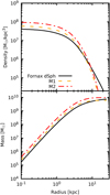 |
Fig. 1 Total density (upper panel) and total mass (lower panel) profiles of our models of the Fornax dSph progenitor M1 (dashed lines) and M2 (dot-dashed lines), and of the Fornax dSph (black solid lines) as estimated by P18. |
2.3 The Milky Way gravitational potential model
In our simulations we model the MW as a frozen gravitational potential, adopting in particular the Johnston et al. (1995, J95) axisymmetric model. Compared to other MW models (e.g. Battaglia et al. 2005; Gibbons et al. 2014; Piffl et al. 2014; Contigiani et al. 2019 and references therein), the J95 model can be considered as a “heavy” MW, having mass of ≃5 × 10¹¹ M⊙ within 50 kpc and ≃2.3 × 10¹² M⊙ within 300 kpc (see Iorio et al. 2019). Thus, adopting the J95 potential, in our simulations we tend to maximize the effects of tidal stripping on Fornax.
The J95 MW model consists of three components (disk, bulge and halo) with total gravitational potential ΦMW,tot(R, z) = Φdisk + Φbulge + Φhalo, where
![Mathematical equation: $\[\Phi_{\text {disk }}(R, z)=-\frac{G M_{\text {disk }}}{\sqrt{R^2+\left(a+\sqrt{z^2+b^2}\right)^2}}\]$](/articles/aa/full_html/2024/10/aa51335-24/aa51335-24-eq28.png) (3)
(3)
for a Miyamoto & Nagai (1975) disk,
![Mathematical equation: $\[\Phi_{\text {bulge }}\left(r_{\mathrm{Gc}}\right)=-\frac{G M_{\text {bulge }}}{r_{\mathrm{Gc}}+c}\]$](/articles/aa/full_html/2024/10/aa51335-24/aa51335-24-eq29.png) (4)
(4)
for a spherical Hernquist (1990) bulge, and
![Mathematical equation: $\[\Phi_{\text {halo }}\left(r_{\mathrm{Gc}}\right)=v_{\text {halo }}^2 \ln \left(r_{\mathrm{Gc}}^2+d^2\right)\]$](/articles/aa/full_html/2024/10/aa51335-24/aa51335-24-eq30.png) (5)
(5)
for a spherical Binney (1981) logarithmic halo. In Equations (3), (4) and (5), ![Mathematical equation: $\[R=\sqrt{x^2+y^2}\]$](/articles/aa/full_html/2024/10/aa51335-24/aa51335-24-eq31.png) and z are Galactocentric cylindrical coordinates, and
and z are Galactocentric cylindrical coordinates, and ![Mathematical equation: $\[r_{\mathrm{Gc}}=\sqrt{R^2+z^2}\]$](/articles/aa/full_html/2024/10/aa51335-24/aa51335-24-eq32.png) is the Galactocentric distance, while the scale and mass parameters are a = 6.5 kpc, b = 0.26 kpc, c = 0.7 kpc, d = 12 kpc, Mbulge = 3.4 × 10¹⁰ M⊙, Mdisk = 1011 M⊙ and vhalo = 128 km/s.
is the Galactocentric distance, while the scale and mass parameters are a = 6.5 kpc, b = 0.26 kpc, c = 0.7 kpc, d = 12 kpc, Mbulge = 3.4 × 10¹⁰ M⊙, Mdisk = 1011 M⊙ and vhalo = 128 km/s.
At variance with some recent works (e.g. Vasiliev et al. 2021; Battaglia et al. 2022; Lilleengen et al. 2023; Koposov et al. 2023), we do not account for the contribution of the Large Magellanic Cloud (LMC) to the Galactic potential (see also Garavito-Camargo et al. 2021). However, as shown in figure D1 of Battaglia et al. (2022), the perturbations induced by the LMC can affect the orbit of Fornax for different initial conditions, but on average its pericentric radius rperi is only slightly altered. Given that the mass loss via tidal stripping is expected to be maximal around rperi, we can safely assume that neglecting the LMC in a heavier MW model does not influence significantly the mass loss of the Fornax dSph with respect to more realistic models including the effect of the LMC (Vasiliev 2024 and references therein).
2.4 N-body code and numerical tests
The simulations presented in this work were performed with the collisionless N-body code FVFPS (FORTRAN version of a fast Poisson solver, Londrillo et al. 2003; Nipoti et al. 2003), based on Dehnen (2002) Poisson solver. As a rule, we adopt a softening length ϵ = 3.1 × 10⁻² kpc. We set the minimum value of the opening parameter θmin, used to control the accuracy of the force evaluation within the tree scheme, to 0.5.
The contribution of the MW is implemented adding the gravitational field derived from the potential ΦMW,tot (Sec. 2.3) to the self-consistent N-body gravitational field −∇Φself. The equations of motion
![Mathematical equation: $\[\ddot{\mathbf{r}}_i=-\nabla\left[\Phi_{\text {self }}\left(\mathbf{r}_i\right)+\Phi_{\text {MW,tot }}\left(\mathbf{r}_i\right)\right]\]$](/articles/aa/full_html/2024/10/aa51335-24/aa51335-24-eq33.png) (6)
(6)
of a particle with position vector ri are propagated with a second order leapfrog scheme using a fixed time-step that we set to 0.01tdyn, where
![Mathematical equation: $\[t_{\mathrm{dyn}} \equiv \sqrt{\frac{8 \pi r_{\text {half }}^3}{3 G M_{\mathrm{tot}}}}\]$](/articles/aa/full_html/2024/10/aa51335-24/aa51335-24-eq34.png) (7)
(7)
is the half-mass dynamical time of the satellite in the initial conditions.
As preliminary tests, we ran simulations of the N-body realizations of models M1 and M2 evolved in isolation for 12 Gyr. For both models we used different resolutions with N spanning a range between 104 and 3 × 10⁶. We found that the isolated N-body systems maintain very well their equilibrium, when simulated with N ≳ 105. The simulations discussed in this work have been performed with N = 106, that gives a good balance between computational time and mass resolution. As an example, in Fig. 2 we show the total density profiles of the initial conditions and of three representative snapshots of the simulation of the isolated M1 model with N = 106. The density profile of the simulated stellar system remains close to the initial profile for the entire time span of the simulation. Small fluctuations below r ≲ 10−1 kpc ≈ 3ϵ are a consequence of shot noise due the poorer sampling in the inner regions, as shown also by the wider Poissonian error bars. Based on these tests, we can robustly ascribe to tidal effects any significant variation of the mass distribution of the N-body systems evolved in the presence of the MW potential.
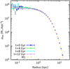 |
Fig. 2 Total density profiles of representative snapshots of the N-body simulation in which an N-body realization of model M1 is evolved in isolation. The dashed line marks the reference initial profile (Eq. (2) with the parameters of model M1). The error bars are computed considering the Poissonian uncertainty on particle counts. |
2.5 Limitations of the models
Our models of the evolution of the Fornax dSph in the MW are simplified in some aspects, which we summarize and discuss here.
As mentioned in Sect. 2.3, it is likely that the adopted MW model is unrealistically heavy. Fornax’s orbit and its tidal stripping history would be different in more realistic, lighter MW models. The gravitational potential of the MW is also assumed to remain the same over the last 12 Gyr, while in the standard hierarchical scenario of structure formation we expect that its mass gradually grows over time via accretion and merging. Moreover, as in our simulations the MW is not represented with particles, the dynamical friction it exerts on the satellite is neglected, so the apocentric distances of the simulated Fornax are underestimated (see Appendix A). All the aforementioned features of the MW model are expected to have the effect of increasing the tidal stripping, because in a more realistic situation (lighter MW and/or operative dynamical friction) the satellite would tend to orbit in regions with weaker tidal forces.
Fornax is modelled as a collisionless system for 12 Gyrs, even if this dwarf galaxy is known to have had a prolonged star formation history that ceased only less than 1 Gyr ago (e.g. de Boer et al. 2012). It follows that Fornax must have had, over most of its lifetime, a gaseous component, that is not included in our models. Though gas behaves differently from the collisionless components during the satellite’s orbit around the MW (for instance, because it suffers also ram-pressure stripping), its presence should not affect significantly our results, because we are interested in the evolution of the stellar mass and not of all the baryonic mass. It is also the case that, in our approach, we do not follow the build-up of the stellar component of Fornax over cosmic time, but, de facto, we assume that all the stars are in place since 12 Gyr ago. Doing so, we tend to enhance the chance that the stars are tidally stripped, because they are exposed to the tidal field of the MW for longer time.
A limitation of the energy-based effective two-component N-body model is that the stellar and DM component share the same isotropic velocity distribution. The effectiveness of tidal stripping is known to depend on the orbits of the stars within the satellite (Kazantzidis et al. 2004; Read et al. 2006), so the fractions of stellar and DM mass lost by Fornax could be different if the two components were allowed to have different velocity distributions. However, at least for the stellar component, the assumption of isotropic distribution function should not be too restrictive, because in the present-day stellar component of Fornax there is no evidence that the velocity distribution deviates from isotropy (P18, Kowalczyk et al. 2019).
The aforementioned simplifying assumptions are justified because the main aim of our study is addressing the specific question of how much stellar mass, at most, Fornax can have lost ceding stars to the MW. Our results are thus robust if they are used to address this question, but cannot provide information on other aspects of the evolution of the Fornax dSph, such as, for instance the star formation history or even the precise stellar mass content at given look-back time. In the following we will thus focus primarily on the question of the fraction of stellar mass lost, for which we can robustly estimate an upper limit. We take advantage of our simulations also to gain insight on some aspects of the evolution of the DM halo of Fornax. In Section 3.3, we quantify the fraction of DM mass lost, but limiting ourselves only to the DM contained within the region in which the dynamical mass can be probed observationally. In Section 3.4, we consider the evolution of the central DM density of the satellite: however, in this respect, our purpose is limited to studying the effect of the pericentric passages on the DM density distribution, with no attempt to include the complex effects of baryon physics on the inner DM distribution in dwarf galaxies (e.g. Nipoti & Binney 2015; Muni et al. 2024, and references therein).
3 Dynamical evolution of Fornax orbiting the Milky Way
3.1 Orbital parameters and N-body simulations
To study the dynamical evolution of the Fornax-like satellite in the MW, we consider two initial conditions for the satellite’s centre of mass, corresponding to two different orbits in the J95 MW gravitational potential, which we will refer to as orbits O1 and O2. In order to define these two orbits, we take the Fornax Gaia-DR3 proper motions, heliocentric distance and sky position from Battaglia et al. (2022), μα = 0.381 ± 0.001 mas yr−1, μδ = −0.358 ± 0.002 mas yr−1, D⊙ = 139.3 ± 2.6 kpc, α(RA) = 39.96667° and δ(DEC) = −34.51361° (assumed without errors), and the systemic line-of-sight velocity from Battaglia et al. (2006), vsys = 54.1 ± 0.4 km s−1. We retrieve the intrinsic position and velocity of Fornax in the Galaxy, defining the Galactic frame of reference as described in Iorio et al. (2019), by assuming that the Sun is at a distance R⊙ = 8.13 ± 0.3 kpc from the Galactic centre (GRAVITY Collaboration 2018), the velocity of the local standard of rest (lsr) is vlsr = 238 ± 9 km s−1 (Schönrich 2012) and the Sun peculiar motion with respect to the lsr is (U⊙, V⊙, W⊙) = (−11.1 ± 1.3, 12.2 ± 2.1, 7.25 ± 0.6) km s−1 (Schönrich et al. 2010). To estimate the effect of the parameter uncertainties on the orbit estimate, we sampled 10 millions orbits randomly drawing the values of the aforementioned parameters, assuming that the associated errors are Gaussian and adding a systematic proper-motion error of 0.017 mas yr−1 (Battaglia et al. 2022). In Fig. 3 we show the resulting distribution of pericentric (rperi) and apocentric (rapo) radii. The orbit O1, that can be considered the “fiducial” orbit of Fornax, has rperi and rapo corresponding to the peak of the distribution shown in Fig. 3. As representative of an extreme orbit, the O2 is chosen among those with the smallest pericentres considering the orbits within 2-σ of the fiducial value in the joint distribution of rperi and rapo (see Fig. 3). Both O1 and O2 are rather eccentric with, respectively, e ≃ 0.5 and e ≃ 0.6, where the eccentricity e is defined in the standard way as
![Mathematical equation: $\[e=\frac{r_{\text {apo }}-r_{\text {peri }}}{r_{\text {apo }}+r_{\text {peri }}}.\]$](/articles/aa/full_html/2024/10/aa51335-24/aa51335-24-eq35.png) (8)
(8)
The initial conditions for the orbits O1 and O2, summarized in Table 2 are recovered by integrating backwards in time, using the PYTHON package GALPY (Bovy 2015) for 12 Gyr in the J95 gravitational potential, starting from the corresponding sets of present-day phase-space coordinates, also given in Table 2.
We present here the results of two simulations, dubbed S1 and S2, in which we have followed for 12 Gyr the evolution of N-body realizations of the models M1 and M2, starting from the initial conditions of orbits O1 and O2, respectively. To compare the simulated trajectory of the Fornax dSph progenitor with the corresponding reference orbits, in each run we evaluated as a function of time the position of the density peak3 of the N-body system, which, hereafter, we will refer to as the centre of the satellite. The latter is determined following the iterative method of Power et al. (2003). In Fig. 4, we plot the trajectories of the N-body satellite’s centre in simulations S1 and S2, against the corresponding point-mass orbits O1 and O2 in the x-y, z-y and x-z planes. The orbit of the Fornax progenitor in the simulation S1 appears to follow closely the corresponding point-mass trajectory O1 for the whole 12 Gyr-integration. The present-day position of the centre of the density distribution (marked in the figure with the purple pentagon) falls very close to its parent position in O1 (indicated by the green cross). The orbit of the (initially) heavier model M2 in simulation S2 starts to show significant discrepancies with respect to its reference orbit O2 at later stages of the evolution (say at around ~7 Gyr), due to the so-called dynamical self-friction4 (Miller et al. 2020) exerted by the tidal tails. The Galactocentric distance (i.e. the distance from the Galactic centre of the satellite’s centre) as a function of time is shown in Fig. 5 for simulations S1 and S2. While in simulation S1 (left panel) no appreciable decay of the apocentre is observable, in simulation S2 (right panel) the apocentre of the orbit has decayed of about 5 kpc after 7 Gyr.
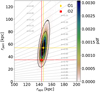 |
Fig. 3 Distribution of Fornax apocentric and pericentric radii from the orbit integration (colour map). The contour levels (thick solid lines) show the area containing the 39%, 86% and 99% of the distribution (corresponding to 2-σ and 3-σ of a 2D Gaussian). The oblique grey lines indicate orbits of a given eccentricity ranging from e = 0 to e = 0.95 with a step δe = 0.05. |
Orbits’ initial conditions.
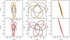 |
Fig. 4 x-y, z-y and x-z projections of Fornax-like O1 (upper panels) and O2 (lower panels) orbits of a point-like mass in the J95 potential (solid lines), and of the trajectories of the satellite’s centre in the corresponding S1 and S2 simulations (yellow and red dots, respectively). The phase-space coordinates of the initial conditions (blue squares) are given in Table 2. The green crosses indicate the observationally determined present-day position of Fornax, which coincides, by construction, with the end point of the reference point-mass orbits. The purple pentagons mark the present-day position of the centre of the satellite in the N-body simulations. |
3.2 Evolution of the satellite total mass distribution
In Figs. 6 and 7, we show snapshots of the particle distributions in the x − y and z − y planes at different times (t = 4, 8 and 12 Gyr) in the simulations S1 and S2, respectively, as well as the trajectories up to said times, as indicated by the yellow and red dotted lines. In each panel, to guide the eye, we superimpose a circle of radius 10 kpc centred in the satellite’s centre at the time of the snapshot. In both simulations, already through the first 4 Gyr of integration the N-body systems have developed long tidal tails. We recall that the particles shown in these figures trace the total mass distribution, with no distinction between stars and DM.
In Fig. 8, we show the evolution of the total density profiles of the satellite in simulations S1 and S2. As a reference, we added in both panels the initial distribution of the parent smooth model (Eq. (2)) and its N-body realization, as well as the profile estimated by P18 as the present-day total density distribution of the Fornax dSph with its 1-σ uncertainty.
The final angle-averaged5 total density profiles of the simulation end-products at 12 Gyr appear compatible with ρP18 below 3 kpc, that is the radius within which we have luminous kinematic tracers. The values of the density in simulation S1 are within 1-σ, while in simulation S2 are slightly above 1-σ of the estimate of P18.
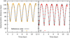 |
Fig. 5 Galactocentric distance of the satellite’s centre as function of time for simulations S1 (left) and S2 (right), respectively. The solid lines mark the trajectory of a point-mass particle with the same initial conditions as the c.o.m. of the satellite in the two simulations. |
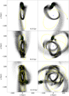 |
Fig. 6 Spatial distribution of the particles of the satellite in the x-y and z-y planes at t = 4, 8 and 12 Gyr for the S1 simulation. Green star: initial position of the satellite’s centre. Dotted lines: trajectory of the satellite’s centre. Blue dot: centre of the MW model. Green circle: 10 kpc radius circumference centred in the satellite’s centre at the time of the snapshot. Here the particles represent the total (stars plus DM) mass distribution. |
3.3 Evolution of the satellite stellar and dark-matter density distributions and mass loss
As discussed in Section 2, we inferred the final stellar and DM distributions of the simulations by tuning the values of the parameters of the portion function (1), so that the final stellar density distribution matches as far as possible the present-day stellar mass distribution of Fornax. In particular, we take as reference the 3D stellar density profile of the best-fitting P18 model.
For each simulation, we found empirically a combination of values of the parameters α, β, γ and ε0 of the portion function (1) such that the final stellar density profile of the simulated satellite is consistent with that estimated for Fornax. The values of the parameters are given in Table 3. The resulting final stellar and DM density profiles are shown in Fig. 9 (lower panels). For the simulation S1, the final stellar density profile matches rather well that of P18 within its error bars (blue shaded area) out to ~2.3 kpc. In S2, the stellar density profile falls within the error bars of the reference density only out to ~1 kpc, while at larger radii the final simulated system has stellar density profiles truncated slightly more sharply than in P18 model (lower right panel). As noted for the total density (see Sect. 3.2), in both cases, the DM profile is slightly higher than that of the reference model (red shaded area) out to about 4 kpc, to fall considerably below it at larger radii. We recall, however, that the comparison with P18 is meaningful only out to ≈3 kpc. In the upper panels of Fig. 9 we also show the initial density profiles of stars and DM. We observe that, in particular for S1, the initial stellar density is characterized by a steeper cusp than its counterpart after 12 Gyr of evolution. As it happens for to the total density profiles, the inner profile, below 10−1 kpc (≈3ϵ) is more noisy and has wider error bars6 due to the poorer sampling.
The tidal forces caused by the interaction with the MW gravitational field strip mass from the Fornax dSph (Choi et al. 2007; Battaglia et al. 2015). To quantify the fractions of stellar and DM mass lost by the simulated satellite while orbiting the Galaxy, we evaluate as a function of time the respective mass content within two control spheres centred on the satellite’s centre: in particular, as in Battaglia et al. (2015), we choose spheres with radii r3 = 3 kpc and r1.6 = 1.6 kpc. In Fig. 10, we present the time evolution of the mass fraction within r3 and r1.6 in simulations S1 and S2 for the stellar and DM components. Our results suggest that Fornax underwent significant DM mass loss, confirming the results obtained by other authors (Battaglia et al. 2015; Genina et al. 2022). However, in both simulations, only the DM mass is significantly affected by the tidal stripping, while the stellar mass remains essentially constant over 12 Gyr of evolution. In simulation S1 there is a flux of stellar mass moving outward from the inner 1.6 kpc zone, but not leaving the sphere of radius r3, the mass within which remains almost constant (see Fig. 10). However, the fraction of stellar mass lost in S1 within 1.6 kpc is only ≈ 4.8%; corresponding to roughly 5 × 10⁵ M⊙. In simulation S2, we observe a more evident loss of mass. DM is heavily stripped away, and at the end of the simulation only 52% of the DM mass is still bound to the galaxy (see Fig. 10). However, as in simulation S1, also in simulation S2 the stellar component is hardly touched; only after 8.5 Gyr there is a non-negligible variation of the stars within 1.6 kpc, which however does not lead to stellar mass loss beyond 3 kpc: the stellar mass within 3 kpc remains constant throughout the simulation. Remarkably, even though the MW model considered here is rather heavy and fixed across the 12 Gyr of simulation, the stellar mass loss remains negligible. The data on the mass loss are reported in Table 4.
From the evolution of the enclosed mass function of DM it is evident that mass loss happens, as expected, mostly when the system approaches the pericentre (the corresponding times are indicated in Fig. 10 by the vertical dotted lines). The increase of the enclosed mass fraction in correspondence of the dotted lines, in particular for S2, might be related to the system encountering mass lost at the previous pericentre passages.
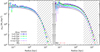 |
Fig. 8 Evolution of the total density profile over 12 Gyr in simulations S1 (left) and S2 (right). The symbols have the same meaning as in Fig. 2. The red and yellow dashed lines mark the initial profiles (models M1 and M2). The gray shaded area is the present-day total density profile of the Fornax dSph estimated by Pascale et al. (2018) with its 1-σ uncertainty. The hatched parts of the graphs indicate regions where the total mass distribution of the Fornax dSph is poorly constrained, because there are no luminous tracers of the gravitational potential. |
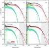 |
Fig. 9 DM (black diamonds) and stellar (green squares) density profiles of the S1 (left) and S2 (right) simulations at t = 0 (upper panels) and 12 Gyr (lower panels). In all panels the cyan and red shaded areas represent, respectively, the stellar and DM density profiles of the Fornax dSph within 1-σ uncertainty, as estimated by P18. The hatched region has the same meaning as in Fig. 8 |
Parameters of the portion function (1).
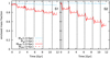 |
Fig. 10 Evolution of the stellar (red lines) and DM (cyan lines) mass fractions of the satellite enclosed within spheres of radius of 1.6 (solid lines) and 3 kpc (dashed lines) for the simulations S1 (left) and S2 (right). The vertical dashed lines mark the times of the passages at the pericentre. |
3.4 Evolution of the satellite central dark matter density ρ150 for different pericentric radii
In the classical dSphs satellites of the MW, the DM density at 150 pc from the centre of the dwarf galaxy (see e.g. Read et al. 2019), ρ150, is found to anticorrelate with the pericentric radius rperi of the dwarf’s orbit (Kaplinghat et al. 2019). Though the robustness (Cardona-Barrero et al. 2023) and interpretation (Andrade et al. 2024) of this anticorrelation is debated, there is general agreement that the dynamical interaction between the dwarf satellites and the MW can contribute to determine the relationship between DM density and orbital properties of the present-day dSphs. For instance, it has been suggested (e.g. Kaplinghat et al. 2019) that an anticorrelation might be produced by the so-called survivor bias: among the dwarfs with small-rperi orbits, only those with high central DM density manage to survive while the others are completely disrupted.
Assuming the parameters of the portion function 𝒫⋆ as given in Table 3, for both simulations S1 and S2 we measured ρ150 and monitored its value as a function of time. The simulations presented in this work, in which the satellite always survives, cannot provide information on the survivor bias scenario. However, given that simulations S1 and S2 are characterized by significantly different rperi (see Table 2), but are designed to have similar final DM density distributions, when interpreted in the context of the ρ150-rperi anticorrelation, they can be used to illustrate, with a clean quantitative example, two important features to be considered when studying the origin the relationship between ρ150 and rperi.
Two MW dSphs with very similar present-day ρ150 can have very different orbits (and values of rperi). In both simulation S1 (with rperi ≈ 54 kpc) and simulation S2 (with rperi ≈ 35 kpc) the final (i.e. present-day) central DM density is ρ150 ≈ 4 × 10⁷ M⊙/pc3 (see Fig. 9).
If the satellites are not completely disrupted, the tidal field of the MW might also have the effect of inducing a correlation between ρ150 and rperi (see also Kaplinghat et al. 2019). This is illustrated by Fig. 11, showing for both simulations S1 and S2, as a function of time, ρ150 normalized to its initial value. In both cases ρ150 decreases with time, but it is apparent that ρ150 decreases at a faster rate in the simulation with lower rperi. Given that the ratio between the pericentric radii is ≈1.6 and the ratio of ρ150 variation is ≈0.7, this effect is opposite, but quantitatively similar, to the empirical anticorrelation (see Cardona-Barrero et al. 2023).
Initial and final mass fractions of stars and DM.
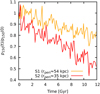 |
Fig. 11 Evolution of the satellite central DM density ρ150, normalized to its value at t = 0, in simulations S1 (yellow line) and S2 (red line). |
4 Discussion
We have dedicated attention to the evolution of the total stellar mass of the Fornax dSph induced by the tidal field of the MW, which provides important constraints for scenarios for the origin of multiple populations (MPs) in GCs. We showed that, during its evolution, Fornax underwent very modest stellar mass loss, thus confirming the results of the simulations of Battaglia et al. (2015). However, it must be stressed that, for the purpose of constraining the stellar mass loss of Fornax, our result is more general than that of Battaglia et al. (2015), who in their simulations (set up in the standard way with a two component N-body model using stellar and DM particles) assumed an initial stellar density distribution of the satellite similar to that observed in Fornax. In our effective two-component simulations, we fix the initial total density distribution of the satellite, but there is no a priori assumption on the stellar density distribution, apart from the relatively weak condition that ρ⋆ cannot exceed ρtot. Thus, though solutions (i.e. choices of the function 𝒫⋆) in which the initial stellar mass of Fornax was significantly higher than its present-day stellar mass would be possible outcomes of our simulations, it turns out that these solutions are excluded when we impose that the end-product of the simulation must have stellar density distribution consistent with the observations. We can thus robustly conclude that the Fornax dSph has retained most of its original stellar content.
In the light of these findings, it remains open the question of explaining both the very high GC specific frequency and the possibility of accommodating the origin of the MPs in GCs in the framework of self-enrichment scenarios, such as the AGB and fast rotating massive stars ones, which assume that, originally, GCs were much more massive than today. At this stage, it is important to stress that caution must be taken when analysing the properties of the GCs and field stars of Fornax. To estimate the amount of this component, Larsen et al. (2012, 2018) assumed an average mass-to-light ratio M/LV = 3.5 (Dubath et al. 1992) to show that about 1/2 of the mass in metal-poor field stars is in GCs, and that the present-day GCs could at most have been by a factor ~4–5 more massive initially then they are now. These data are particularly impressive if compared to the ratio between the total mass in MW GCs and the stellar halo, of the order of a few per cent only. However, the total stellar mass of Fornax is still significantly affected by uncertainties, in particular regarding the assumed M/LV ratio, for which SSP models for a standard IMF predict lower values, M/LV = 2 (e.g. Strader et al. 2011).
By means of up-to-date photometric data of Galactic GCs, the recent estimate of Baumgardt et al. (2020) indicates an average mass-to-light ratio of M/LV=1.83. Still, this value is subject to various uncertainties, such as stellar age, metallicity and the impact of internal dynamical processes, such as mass segregation (Baumgardt et al. 2020 and references therein). However, if the properties of Galactic GCs were similar to the ones of their Fornax homologous, this M/LV value would imply a 1.9 increase in the ratio between field stars and GCs and an upper limit of 9.6 between the total GC mass and field stars, bringing it in better agreement with the values expected in the MPs formation scenarios discussed above.
In the future, it will be important to develop new models to study the mass of such clusters throughout their history and, starting from a set of different initial conditions, which evolutionary path led to the current configuration. These models need to take into account the influence of the cosmological environment, to compute how the time-varying tidal field emerging from the past merging history has contributed to cause the dynamical evolution of the Fornax clusters, as already performed for MW GCs by Rodriguez et al. (2022). A significant result in this field is the recent one by Moreno-Hilario et al. (2024), who show how the disruption processes of GCs are sensitive to the mass and density of the host galaxy and supporting larger GC specific frequencies in dwarf galaxies. Moreover, future models should also include the effects of stellar evolution on the (baryonic) mass loss.
Khalaj & Baumgardt (2016) conjecture that few hypervelocity stars escaping the GCs of Fornax might be accelerated by other evolutionary processes such as gas expulsion from GCs (the latter also contributing to the total mass loss). Indeed, other studies have indicated that intense stellar feedback may lead to significant loss of residual gas from GCs (e.g. Baumgardt & Kroupa 2007; Calura et al. 2015; Silich & Tenorio-Tagle 2018). In the case of Fornax, to achieve the large velocities necessary for stellar expulsion, gas loss has to be significant and rapid, i.e. to occur on timescales ≤ 105 yr. Assessing this possibility requires dedicated simulations to explore a wide parameter space, including stellar feedback prescriptions, star formation efficiency and some GCs structural properties. Moreover, a further, necessary condition for the mechanism proposed by Khalaj & Baumgardt (2016) to be effective is that the Fornax dark halo is cuspy (or with a small core), which is not favoured by some recent dynamical models (Pascale et al. 2018; Battaglia & Nipoti 2022, and references therein).
5 Summary and conclusions
We have studied the dynamical evolution of the Fornax dSph with effective multi-component N–body simulations. Using two different orbits in the MW potential, based on state-of-the art estimates of Fornax’s orbital parameters, we find for both orbits considerable DM mass loss along 12 Gyr integration time, and rather mild orbital decay induced by dynamical self-friction.
At the end of the simulations, the simulated Fornax-like satellite is located in a position consistent with the present-day observed position of Fornax. The final stellar density profile of the simulated satellite is (at least in one case) well within the error bars of the model of P18. The DM component suffers substantial depletion due to tidal stripping in the Galactic potential, losing a fraction of between the 20 and the 50% within a 3 kpc radius. The central DM density of the simulated satellite ρ150, measured at 150 pc from the centre, decreases more in the orbit with the smaller pericentric radius rperi. Thus, our simulations provide further indications that an ρ150-rperi anticorrelation is not a straightforward consequence of the dynamical interaction of the dwarf satellites with the tidal field of the MW.
The main result of this work is that, though our initial conditions would permit a wide variety of initial stellar mass distributions for Fornax, for the final stellar and DM density distributions to be consistent with the ones observed at the present day, the stellar mass loss must have been very low (≲3%). Thus, it appears rather unlikely that loss of mass from Fornax to the MW could be the explanation of the anomalously high fraction of stellar mass that in Fornax resides in GCs, which remains a problem (despite the significant uncertainty in the adopted GC mass-to-light ratio) for GC formation scenarios that postulate that GCs were originally much more massive.
Acknowledgements
PFDC wishes to acknowledge funding by “Fondazione Cassa di Risparmio di Firenze” under the project HIPERCRHEL for the use of high performance computing resources at the University of Firenze. The research activities described in this paper have been co-funded by the European Union – NextGenerationEU within PRIN 2022 project no. 20229YBSAN – Globular clusters in cosmological simulations and in lensed fields: from their birth to the present epoch. G.I. acknowledges financial support under the National Recovery and Resilience Plan (NRRP), Mission 4, Component 2, Investment 1.4, – Call for tender No. 3138 of 18/12/2021 of Italian Ministry of University and Research funded by the European Union -– NextGenerationEU.
Appendix A Dynamical friction tests
To test the possible influence of dynamical friction on the orbit of the Fornax dSph, we performed additional single particle integrations using GALPY, where a test mass Mtot orbits according to the equations of motion
![Mathematical equation: $\[\ddot{\mathbf{r}}=-\nabla \Phi_{\mathrm{MW}, \text { tot }}(\mathbf{r})+\mathbf{a}_{D F},\]$](/articles/aa/full_html/2024/10/aa51335-24/aa51335-24-eq40.png) (A.1)
(A.1)
where
![Mathematical equation: $\[\mathbf{a}_{\mathrm{DF}}=-2 \pi G^2 M_{\mathrm{tot}} \rho(\mathbf{r}) \ln \left(1+\Lambda^2\right)\left[\operatorname{erf}(X)-\frac{2 X^2}{\sqrt{\pi}} \exp \left(-X^2\right)\right] \frac{\mathbf{v}}{v^3}\]$](/articles/aa/full_html/2024/10/aa51335-24/aa51335-24-eq41.png) (A.2)
(A.2)
is the deceleration produced by dynamical friction (Petts et al. 2016). Here ρ(r) is the total mass density of the MW at r, v = ![Mathematical equation: $\[\dot{\mathbf{r}}\]$](/articles/aa/full_html/2024/10/aa51335-24/aa51335-24-eq42.png) and
and ![Mathematical equation: $\[X=v /(\sqrt{2} \sigma)\]$](/articles/aa/full_html/2024/10/aa51335-24/aa51335-24-eq43.png) , with σ(r) the velocity dispersion at r (i.e. the local Maxwellian approximation is assumed) evaluated solving the Jeans equations for the MW potential and density (see Bovy 2015 and references therein). In Equation (A.2), in order to take into account that the satellite is extended7, Λ is defined as
, with σ(r) the velocity dispersion at r (i.e. the local Maxwellian approximation is assumed) evaluated solving the Jeans equations for the MW potential and density (see Bovy 2015 and references therein). In Equation (A.2), in order to take into account that the satellite is extended7, Λ is defined as
![Mathematical equation: $\[\Lambda=\frac{r_{\mathrm{Gal}}}{\max \left[r_{\mathrm{sat}}, \frac{G M_{\mathrm{tot}}}{v^2}\right]},\]$](/articles/aa/full_html/2024/10/aa51335-24/aa51335-24-eq44.png) (A.3)
(A.3)
where rGal and rsat are the scale radii of the Galaxy and the satellite, which we take to be 12 kpc and 4.3 kpc, respectively.
In the left panel of Fig. A.1 we show the Galactocentric distance as a function of time for the orbit O1 and for a particle of mass Mtot = 7.2 × 10⁹ M⊙ (the total mass of model M1; Section 2.2) orbiting in the same gravitational potential and having the same phase-space coordinates at 12 Gyr, but under the effect of dynamical friction (Eq. A.1). The analogous comparison for the orbit O2 is shown in the right panel of Fig. A.1, where the orbit with dynamical friction is for a particle of mass Mtot = 1.13 × 10¹⁰ M⊙ (the total mass of model M2; Section 2.2). The Galactocentric distances for both models match rather well the parent trajectories without dynamical friction for, at least, the last 3 Gyr. At earlier times the orbits with and without dynamical friction differ significantly: the initial apocentre is larger in the presence than in the absence of dynamical friction, of about a factor 1.25 in the case of O1 and a factor 1.5 in the case of O2.
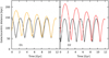 |
Fig. A.1 Orbital decay with dynamical friction. Left panel. Galacto-centric distance as a function of time for the orbit O1 (black curve) and for a particle of mass Mtot = 7.2 × 10⁹ M⊙ orbiting in the same gravitational potential and having the same phase-space coordinates at 12 Gyr, but under the effect of dynamical friction (yellow curve). Right panel: same as left panel, but for the orbit O2 (black curve) and the corresponding orbit with dynamical friction (red curve) for a particle of mass Mtot = 1.13 × 10¹⁰ M⊙. |
As expected (Miller et al. 2020), in the single particle orbital integration including dynamical friction, the orbital decay of the Fornax dSph is significantly larger than that in the N-body experiments including only dynamical self-friction (see Fig. 5). However, the pericentre, where most of the mass stripping happens, is almost unaffected by dynamical friction. We should also note that, since in our experiments the point mass Mtot, representing the total mass of the satellite, is kept constant, the strength of the dynamical friction is systematically overestimated. To explore this processes more in detail one should run full N-body simulations where the MW is also modelled using particles, in the same spirit as, for example, Mori et al. (2024).
References
- Andrade, K. E., Kaplinghat, M., & Valli, M. 2024, MNRAS, 532, 4157 [NASA ADS] [CrossRef] [Google Scholar]
- Battaglia, G., & Nipoti, C. 2022, Nat. Astron., 6, 659 [NASA ADS] [CrossRef] [Google Scholar]
- Battaglia, G., Helmi, A., Morrison, H., et al. 2005, MNRAS, 364, 433 [NASA ADS] [CrossRef] [Google Scholar]
- Battaglia, G., Tolstoy, E., Helmi, A., et al. 2006, A&A, 459, 423 [NASA ADS] [CrossRef] [EDP Sciences] [Google Scholar]
- Battaglia, G., Sollima, A., & Nipoti, C. 2015, MNRAS, 454, 2401 [NASA ADS] [CrossRef] [Google Scholar]
- Battaglia, G., Taibi, S., Thomas, G. F., & Fritz, T. K. 2022, A&A, 657, A54 [NASA ADS] [CrossRef] [EDP Sciences] [Google Scholar]
- Baumgardt, H., & Kroupa, P. 2007, MNRAS, 380, 1589 [NASA ADS] [CrossRef] [Google Scholar]
- Baumgardt, H., Sollima, A., & Hilker, M. 2020, PASA, 37, e046 [Google Scholar]
- Binney, J. 1981, MNRAS, 196, 455 [NASA ADS] [Google Scholar]
- Bird, S. A., Xue, X.-X., Liu, C., et al. 2021, ApJ, 919, 66 [NASA ADS] [CrossRef] [Google Scholar]
- Borukhovetskaya, A., Errani, R., Navarro, J. F., Fattahi, A., & Santos-Santos, I. 2022, MNRAS, 509, 5330 [Google Scholar]
- Bovy, J. 2015, ApJS, 216, 29 [NASA ADS] [CrossRef] [Google Scholar]
- Bullock, J. S., & Johnston, K. V. 2005, ApJ, 635, 931 [Google Scholar]
- Calura, F., Ciotti, L., & Nipoti, C. 2014, MNRAS, 440, 3341 [NASA ADS] [CrossRef] [Google Scholar]
- Calura, F., Few, C. G., Romano, D., & D’Ercole, A. 2015, ApJ, 814, L14 [NASA ADS] [CrossRef] [Google Scholar]
- Calura, F., D’Ercole, A., Vesperini, E., Vanzella, E., & Sollima, A. 2019, MNRAS, 489, 3269 [Google Scholar]
- Cardona-Barrero, S., Battaglia, G., Nipoti, C., & Di Cintio, A. 2023, MNRAS, 522, 3058 [CrossRef] [Google Scholar]
- Choi, J.-H., Weinberg, M. D., & Katz, N. 2007, MNRAS, 381, 987 [NASA ADS] [CrossRef] [Google Scholar]
- Contigiani, O., Rossi, E. M., & Marchetti, T. 2019, MNRAS, 487, 4025 [NASA ADS] [CrossRef] [Google Scholar]
- D’Antona, F., Vesperini, E., D’Ercole, A., et al. 2016, MNRAS, 458, 2122 [Google Scholar]
- Darragh-Ford, E., Nadler, E. O., McLaughlin, S., & Wechsler, R. H. 2021, ApJ, 915, 48 [CrossRef] [Google Scholar]
- de Boer, T. J. L., Tolstoy, E., Hill, V., et al. 2012, A&A, 544, A73 [NASA ADS] [CrossRef] [EDP Sciences] [Google Scholar]
- Decressin, T., Meynet, G., Charbonnel, C., Prantzos, N., & Ekström, S. 2007, A&A, 464, 1029 [NASA ADS] [CrossRef] [EDP Sciences] [Google Scholar]
- Decressin, T., Baumgardt, H., & Kroupa, P. 2008, A&A, 492, 101 [NASA ADS] [CrossRef] [EDP Sciences] [Google Scholar]
- Dehnen, W. 2002, J. Computat. Phys., 179, 27 [CrossRef] [Google Scholar]
- D’Ercole, A., Vesperini, E., D’Antona, F., McMillan, S. L. W., & Recchi, S. 2008, MNRAS, 391, 825 [CrossRef] [Google Scholar]
- Dubath, P., Meylan, G., & Mayor, M. 1992, ApJ, 400, 510 [NASA ADS] [CrossRef] [Google Scholar]
- Elias, L. M., Sales, L. V., Helmi, A., & Hernquist, L. 2020, MNRAS, 495, 29 [NASA ADS] [CrossRef] [Google Scholar]
- Elmegreen, B. G. 1999, Ap&SS, 269, 469 [NASA ADS] [CrossRef] [Google Scholar]
- Errani, R., Penarrubia, J., & Tormen, G. 2015, MNRAS, 449, L46 [Google Scholar]
- Garavito-Camargo, N., Besla, G., Laporte, C. F. P., et al. 2021, ApJ, 919, 109 [NASA ADS] [CrossRef] [Google Scholar]
- Genina, A., Read, J. I., Fattahi, A., & Frenk, C. S. 2022, MNRAS, 510, 2186 [Google Scholar]
- Gibbons, S. L. J., Belokurov, V., & Evans, N. W. 2014, MNRAS, 445, 3788 [NASA ADS] [CrossRef] [Google Scholar]
- GRAVITY Collaboration (Abuter, R., et al.) 2018, A&A, 615, L15 [NASA ADS] [CrossRef] [EDP Sciences] [Google Scholar]
- Hernquist, L. 1990, ApJ, 356, 359 [Google Scholar]
- Huang, K.-W., & Koposov, S. E. 2021, MNRAS, 500, 986 [Google Scholar]
- Iorio, G., Nipoti, C., Battaglia, G., & Sollima, A. 2019, MNRAS, 487, 5692 [CrossRef] [Google Scholar]
- Johnston, K. V., Spergel, D. N., & Hernquist, L. 1995, ApJ, 451, 598 [NASA ADS] [CrossRef] [Google Scholar]
- Kaplinghat, M., Valli, M., & Yu, H.-B. 2019, MNRAS, 490, 231 [NASA ADS] [CrossRef] [Google Scholar]
- Kazantzidis, S., Magorrian, J., & Moore, B. 2004, ApJ, 601, 37 [NASA ADS] [CrossRef] [Google Scholar]
- Khalaj, P., & Baumgardt, H. 2016, MNRAS, 457, 479 [NASA ADS] [CrossRef] [Google Scholar]
- Koposov, S. E., Erkal, D., Li, T. S., et al. 2023, MNRAS, 521, 4936 [NASA ADS] [CrossRef] [Google Scholar]
- Kowalczyk, K., del Pino, A., Łokas, E. L., & Valluri, M. 2019, MNRAS, 482, 5241 [NASA ADS] [CrossRef] [Google Scholar]
- Kroupa, P. 2001, MNRAS, 322, 231 [NASA ADS] [CrossRef] [Google Scholar]
- Kruijssen, J. M. D., Pfeffer, J. L., Reina-Campos, M., Crain, R. A., & Bastian, N. 2019, MNRAS, 486, 3180 [Google Scholar]
- Larsen, S. S., Strader, J., & Brodie, J. P. 2012, A&A, 544, L14 [NASA ADS] [CrossRef] [EDP Sciences] [Google Scholar]
- Larsen, S. S., Brodie, J. P., Wasserman, A., & Strader, J. 2018, A&A, 613, A56 [NASA ADS] [CrossRef] [EDP Sciences] [Google Scholar]
- Letarte, B., Hill, V., Jablonka, P., et al. 2006, A&A, 453, 547 [NASA ADS] [CrossRef] [EDP Sciences] [Google Scholar]
- Lilleengen, S., Petersen, M. S., Erkal, D., et al. 2023, MNRAS, 518, 774 [Google Scholar]
- Londrillo, P., Nipoti, C., & Ciotti, L. 2003, Mem. Soc. Astron. Ital. Suppl., 1, 18 [Google Scholar]
- Massari, D., Aguado-Agelet, F., Monelli, M., et al. 2023, A&A, 680, A20 [NASA ADS] [CrossRef] [EDP Sciences] [Google Scholar]
- Miller, T. B., van den Bosch, F. C., Green, S. B., & Ogiya, G. 2020, MNRAS, 495, 4496 [Google Scholar]
- Milone, A. P., Marino, A. F., Piotto, G., et al. 2015, MNRAS, 447, 927 [NASA ADS] [CrossRef] [Google Scholar]
- Miyamoto, M., & Nagai, R. 1975, PASJ, 27, 533 [NASA ADS] [Google Scholar]
- Moreno-Hilario, E., Martinez-Medina, L. A., Li, H., Souza, S. O., & Pérez-Villegas, A. 2024, MNRAS, 527, 2765 [Google Scholar]
- Mori, A., Di Matteo, P., Salvadori, S., et al. 2024, A&A, in press, https://doi.org/10.1051/0004-6361/202449291 [Google Scholar]
- Mucciarelli, A., & Massari, D. 2023, Mem. Soc. Astron. Ital., 94, 173 [NASA ADS] [Google Scholar]
- Mulder, W. A. 1983, A&A, 117, 9 [NASA ADS] [Google Scholar]
- Muni, C., Pontzen, A., Read, J. I., et al. 2024, arXiv e-prints [arXiv:2407.14579] [Google Scholar]
- Nipoti, C., & Binney, J. 2015, MNRAS, 446, 1820 [NASA ADS] [CrossRef] [Google Scholar]
- Nipoti, C., Londrillo, P., & Ciotti, L. 2003, MNRAS, 342, 501 [Google Scholar]
- Nipoti, C., Londrillo, P., & Ciotti, L. 2006, MNRAS, 370, 681 [NASA ADS] [CrossRef] [Google Scholar]
- Nipoti, C., Cherchi, G., Iorio, G., & Calura, F. 2021, MNRAS, 503, 4221 [NASA ADS] [CrossRef] [Google Scholar]
- Pace, A. B., Walker, M. G., Koposov, S. E., et al. 2021, ApJ, 923, 77 [NASA ADS] [CrossRef] [Google Scholar]
- Pascale, R., Posti, L., Nipoti, C., & Binney, J. 2018, MNRAS, 480, 927 [Google Scholar]
- Petts, J. A., Read, J. I., & Gualandris, A. 2016, MNRAS, 463, 858 [NASA ADS] [CrossRef] [Google Scholar]
- Piffl, T., Binney, J., McMillan, P. J., et al. 2014, MNRAS, 445, 3133 [CrossRef] [Google Scholar]
- Power, C., Navarro, J. F., Jenkins, A., et al. 2003, MNRAS, 338, 14 [Google Scholar]
- Read, J. I., Wilkinson, M. I., Evans, N. W., Gilmore, G., & Kleyna, J. T. 2006, MNRAS, 366, 429 [NASA ADS] [CrossRef] [Google Scholar]
- Read, J. I., Walker, M. G., & Steger, P. 2019, MNRAS, 484, 1401 [NASA ADS] [CrossRef] [Google Scholar]
- Rodriguez, C. L., Weatherford, N. C., Coughlin, S. C., et al. 2022, ApJS, 258, 22 [NASA ADS] [CrossRef] [Google Scholar]
- Salpeter, E. E. 1955, ApJ, 121, 161 [Google Scholar]
- Schechter, P. 1976, ApJ, 203, 297 [Google Scholar]
- Schönrich, R. 2012, MNRAS, 427, 274 [Google Scholar]
- Schönrich, R., Binney, J., & Dehnen, W. 2010, MNRAS, 403, 1829 [NASA ADS] [CrossRef] [Google Scholar]
- Shchelkanova, G., Hayashi, K., & Blinnikov, S. 2021, ApJ, 909, 147 [NASA ADS] [CrossRef] [Google Scholar]
- Silich, S., & Tenorio-Tagle, G. 2018, MNRAS, 478, 5112 [NASA ADS] [CrossRef] [Google Scholar]
- Strader, J., Caldwell, N., & Seth, A. C. 2011, AJ, 142, 8 [NASA ADS] [CrossRef] [Google Scholar]
- Vasiliev, E. 2024, MNRAS, 527, 437 [Google Scholar]
- Vasiliev, E., Belokurov, V., & Erkal, D. 2021, MNRAS, 501, 2279 [NASA ADS] [CrossRef] [Google Scholar]
- Wang, M.-Y., Strigari, L. E., Lovell, M. R., Frenk, C. S., & Zentner, A. R. 2016, MNRAS, 457, 4248 [NASA ADS] [CrossRef] [Google Scholar]
- Wang, M. Y., Koposov, S., Drlica-Wagner, A., et al. 2019, ApJ, 875, L13 [Google Scholar]
Local spiral galaxies typically have SN ≤ 1, whereas ellipticals, dwarf ellipticals and S0 galaxies show GC specific frequencies in the range 2 ≤ SN ≤ 6.
As it is usual in simulations with substantial tidal stripping, the centre of mass cannot be used as centre of the satellite, because of its dependence on the geometry of the tidal tails.
The effect of the dynamical friction exerted by the host galaxy on the satellite is absent by construction in our simulations in which the host system is modelled as a fixed gravitational potential (see Appendix A for a discussion).
The density profiles have been evaluated within spherical shells, which is justified because the final axial ratios within a sphere enclosing the 80% of the total initial mass (see Nipoti et al. 2006 for the numerical procedure) are c/a = b/a = 0.99 for S1 and c/a = 0.99 and b/a = 0.98 for S2, where c ≤ b ≤ a are the principal axes of the inertia tensor.
The errors on the stellar and DM density are computed, respectively, as Δρ⋆ = (ρ*/ρtot)Δρtot and ΔρDM = (ρDM/ρtot)Δρtot, where Δρtot is the error on the total density.
A more refined way to evaluate the dynamical friction on an extended object is given by the model of Mulder (1983), in which the satellite suffers a drag force that is augmented by the interaction between its density profile and the trailing wake. The satellite deformation and possibly the mass stripping induced by the background density of the parent galaxy are also accounted for, leading to a contribution to the slowing down that is however considerably lower than that of the pure dynamical friction.
All Tables
All Figures
|
Fig. 1 Total density (upper panel) and total mass (lower panel) profiles of our models of the Fornax dSph progenitor M1 (dashed lines) and M2 (dot-dashed lines), and of the Fornax dSph (black solid lines) as estimated by P18. |
| In the text | |
|
Fig. 2 Total density profiles of representative snapshots of the N-body simulation in which an N-body realization of model M1 is evolved in isolation. The dashed line marks the reference initial profile (Eq. (2) with the parameters of model M1). The error bars are computed considering the Poissonian uncertainty on particle counts. |
| In the text | |
|
Fig. 3 Distribution of Fornax apocentric and pericentric radii from the orbit integration (colour map). The contour levels (thick solid lines) show the area containing the 39%, 86% and 99% of the distribution (corresponding to 2-σ and 3-σ of a 2D Gaussian). The oblique grey lines indicate orbits of a given eccentricity ranging from e = 0 to e = 0.95 with a step δe = 0.05. |
| In the text | |
|
Fig. 4 x-y, z-y and x-z projections of Fornax-like O1 (upper panels) and O2 (lower panels) orbits of a point-like mass in the J95 potential (solid lines), and of the trajectories of the satellite’s centre in the corresponding S1 and S2 simulations (yellow and red dots, respectively). The phase-space coordinates of the initial conditions (blue squares) are given in Table 2. The green crosses indicate the observationally determined present-day position of Fornax, which coincides, by construction, with the end point of the reference point-mass orbits. The purple pentagons mark the present-day position of the centre of the satellite in the N-body simulations. |
| In the text | |
|
Fig. 5 Galactocentric distance of the satellite’s centre as function of time for simulations S1 (left) and S2 (right), respectively. The solid lines mark the trajectory of a point-mass particle with the same initial conditions as the c.o.m. of the satellite in the two simulations. |
| In the text | |
|
Fig. 6 Spatial distribution of the particles of the satellite in the x-y and z-y planes at t = 4, 8 and 12 Gyr for the S1 simulation. Green star: initial position of the satellite’s centre. Dotted lines: trajectory of the satellite’s centre. Blue dot: centre of the MW model. Green circle: 10 kpc radius circumference centred in the satellite’s centre at the time of the snapshot. Here the particles represent the total (stars plus DM) mass distribution. |
| In the text | |
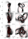 |
Fig. 7 Same as in Fig. 6, but for the simulation S2. |
| In the text | |
|
Fig. 8 Evolution of the total density profile over 12 Gyr in simulations S1 (left) and S2 (right). The symbols have the same meaning as in Fig. 2. The red and yellow dashed lines mark the initial profiles (models M1 and M2). The gray shaded area is the present-day total density profile of the Fornax dSph estimated by Pascale et al. (2018) with its 1-σ uncertainty. The hatched parts of the graphs indicate regions where the total mass distribution of the Fornax dSph is poorly constrained, because there are no luminous tracers of the gravitational potential. |
| In the text | |
|
Fig. 9 DM (black diamonds) and stellar (green squares) density profiles of the S1 (left) and S2 (right) simulations at t = 0 (upper panels) and 12 Gyr (lower panels). In all panels the cyan and red shaded areas represent, respectively, the stellar and DM density profiles of the Fornax dSph within 1-σ uncertainty, as estimated by P18. The hatched region has the same meaning as in Fig. 8 |
| In the text | |
|
Fig. 10 Evolution of the stellar (red lines) and DM (cyan lines) mass fractions of the satellite enclosed within spheres of radius of 1.6 (solid lines) and 3 kpc (dashed lines) for the simulations S1 (left) and S2 (right). The vertical dashed lines mark the times of the passages at the pericentre. |
| In the text | |
|
Fig. 11 Evolution of the satellite central DM density ρ150, normalized to its value at t = 0, in simulations S1 (yellow line) and S2 (red line). |
| In the text | |
|
Fig. A.1 Orbital decay with dynamical friction. Left panel. Galacto-centric distance as a function of time for the orbit O1 (black curve) and for a particle of mass Mtot = 7.2 × 10⁹ M⊙ orbiting in the same gravitational potential and having the same phase-space coordinates at 12 Gyr, but under the effect of dynamical friction (yellow curve). Right panel: same as left panel, but for the orbit O2 (black curve) and the corresponding orbit with dynamical friction (red curve) for a particle of mass Mtot = 1.13 × 10¹⁰ M⊙. |
| In the text | |
Current usage metrics show cumulative count of Article Views (full-text article views including HTML views, PDF and ePub downloads, according to the available data) and Abstracts Views on Vision4Press platform.
Data correspond to usage on the plateform after 2015. The current usage metrics is available 48-96 hours after online publication and is updated daily on week days.
Initial download of the metrics may take a while.