| Issue |
A&A
Volume 699, July 2025
|
|
|---|---|---|
| Article Number | A347 | |
| Number of page(s) | 21 | |
| Section | Galactic structure, stellar clusters and populations | |
| DOI | https://doi.org/10.1051/0004-6361/202554826 | |
| Published online | 22 July 2025 | |
Chemo-dynamics of the stellar component of the Sculptor dwarf galaxy
II. Dynamical properties and dark matter halo density
1
Instituto de Astrofísica de Canarias,
Calle Vía Láctea s/n, 38206 La Laguna,
Santa Cruz de Tenerife,
Spain
2
Universidad de La Laguna,
Avda. Astrofísico Francisco Sánchez 38205 La Laguna,
Santa Cruz de Tenerife,
Spain
3
INAF – Osservatorio di Astrofisica e Scienza dello Spazio di Bologna,
Via Piero Gobetti 93/3,
40129
Bologna,
Italy
4
Dipartimento di Fisica e Astronomia “Augusto Righi” – DIFA, Alma Mater Studiorum – Universita‘ di Bologna,
via Gobetti 93/2,
40129
Bologna,
Italy
5
University of Surrey,
Guildford GU2 7XH,
UK
6
Kapteyn Astronomical Institute, University of Groningen,
PO Box 800,
9700
AV Groningen,
The Netherlands
★ Corresponding author: This email address is being protected from spambots. You need JavaScript enabled to view it.
Received:
28
March
2025
Accepted:
10
June
2025
Abstract
Dwarf galaxy satellites of the Milky Way are excellent laboratories for testing dark matter (DM) models and baryonic feedback implementation in simulations. The Sculptor “classical” dwarf spheroidal galaxy, a system with two distinct stellar populations and high-quality data, offers a remarkable opportunity to study DM distributions in these galaxies. However, inferences from dynamical modeling in the literature have led to discrepant results. In this work, we infer the DM halo density distribution of Sculptor, applying a method based on spherically symmetric distribution functions depending on actions to fit the stellar structural and kinematic properties of Sculptor. The galaxy is represented via four components: two distinct stellar populations based on distribution functions, tracers within a fixed and dominant DM potential, and the contribution of a third stellar component that accounts for possible sources of contamination. The model-data comparison accounts for the kinematics and metallicities of individual stars rather than relying on binned profiles, allowing us to assign probabilities of membership to each star. This is the most general approach employed to date to model Sculptor, and we applied it on the largest available set of spectroscopic data, which have not been previously analyzed with this objective. We find the DM distribution of Sculptor to have a logarithmic inner slope of γ = 0.39−0.26+0.23 and a scale radius of rs = 0.79−0.17+0.38kpc at a 1σ confidence level. Our results show that the Sculptor DM density profile deviates from predictions of DM-only simulations at a 3σ level over a large range of radii. The dynamical-to-luminous mass ratio is around 13 at the 3D half-light radius and 154 at 2 kpc, the outermost radius with observed stars in our dataset. Our analysis suggests that the velocity distribution of Sculptor’s two main stellar components is isotropic in the center and becomes radially anisotropic in the outskirts. Additionally, we provide predictions for the projected radial and tangential velocity dispersion profiles. We also present updated DM annihilation and decay J – and D-factors, for which we find J = 18.15−0.12+0.11 and D = 18.07−0.10+0.10 for an angular aperture of 0.5 degrees.
Key words: galaxies: dwarf / galaxies: halos / galaxies: individual: Sculptor / galaxies: kinematics and dynamics / Local Group / dark matter
© The Authors 2025
 Open Access article, published by EDP Sciences, under the terms of the Creative Commons Attribution License (https://creativecommons.org/licenses/by/4.0), which permits unrestricted use, distribution, and reproduction in any medium, provided the original work is properly cited.
This article is published in open access under the Subscribe to Open model. This email address is being protected from spambots. You need JavaScript enabled to view it. to support open access publication.
1 Introduction
In the current Λ cold dark matter (Λ CDM) cosmological model, pure N-body cosmological simulations predict that dark matter (DM) forms halos characterized by cuspy Navarro et al. (1997, NFW) density profiles. However, this prediction stands in contrast to a wealth of observational evidence indicating the presence of constant-density cores in the central regions of many low surface brightness galaxies (Gentile et al. 2004; Simon et al. 2005; de Blok et al. 2008; Walker & Peñarrubia 2011; Pascale et al. 2018; Leung et al. 2021, among others). This is known as the cusp-core problem. To address this tension, as well as others not discussed in this article, modifications to the Λ CDM model have been proposed, including self-interacting DM (SIDM) (Carlson et al. 1992) and fuzzy DM (Hu et al. 2000), among others (see Bullock & Boylan-Kolchin 2017, and references therein). Real galaxies, however, are not merely collections of collisionless DM particles, as they also contain stars, dust, and gas. In the past years, two main mechanisms have been identified through which the baryonic component can influence the distribution of DM in the inner regions of a halo: via violent and rapid variations of the gravitational potential due to gas expulsion as a consequence of supernova feedback (e.g., Mashchenko et al. 2006; Pontzen & Governato 2014) or via dynamical friction with fragmented gas clouds even before stellar feedback takes place (e.g., El-Zant et al. 2001; Nipoti & Binney 2015). Dynamical friction between massive gas clouds and DM is efficient enough to form cores in galaxies with a gas mass of Mgas=107 M⊙ and a DM halo virial mass of Mhalo=109 M⊙, i.e. in the regime of dwarf spheroidals (dSphs), as shown by adiabatic non-cosmological simulations (Nipoti & Binney 2015). As for the impact of stellar feedback, typically some degree of core formation occurs in simulations that resolve and model star formation in high-density gas, such as NIHAO (Wang et al. 2015) and FIRE (Hopkins et al. 2014). The process is particularly efficient in galaxies where the ratio of stellar-tohalo mass is 10−3 < M⋆/Mhalo < 10−2 (Di Cintio et al. 2014b; Oñorbe et al. 2015). However, the scales of the smallest and most DM dominated galaxies, for example “classical” dSphs and ultra-faint dwarfs (UFDs), are particularly tricky as this regime of masses and sizes approaches the mass and spatial resolution limits of simulations (see discussion by Sales et al. 2022). In fact, higher-resolution non-cosmological hydrodynamical simulations are able to form cores in the regime of faint galaxies down to M⋆/Mhalo ≈ 10−4 at log (M⋆[M⊙])=4 (Read et al. 2016; Pascale et al. 2023), but only in systems with bursty and prolonged star formation histories (SFHs) up to the present. Hence, several aspects remain debated, such as the expected core sizes, the minimum mass to form a core and how core formation relates to the galaxy’s SFH. In summary, while the inclusion of baryons in the simulations offers a promising solution to the cusp-core problem, it remains unclear whether they can fully reconcile all observations with the Λ CDM model predictions. Therefore, accurate and precise inferences of the DM density profiles of galaxies over a range of stellar masses and SFHs are clearly essential to effectively constrain these models.
Local Group (LG) dwarf galaxies are thus precious laboratories in this context. These galaxies lie in the M⋆/Mhalo regime (Battaglia & Nipoti 2022, and references therein) in which the efficacy of stellar feedback in turning cusps into cores varies from extremely low to strong, depending on the exact correspondence between M⋆ and Mhalo. Furthermore, they display a variety of SFHs (Gallart et al. 2015), in particular when considering M31 and isolated LG dwarfs. The classical dSphs satellites of the Milky Way are the best studied among the LG dwarf galaxies due to the amount of observational data that can be gathered for these systems with current facilities. However, they lack gas, leaving stars as the only tracers of the gravitational potential. This poses a significant complication, as the anisotropy of stellar motions is degenerate with the underlying mass distribution. Nevertheless, these systems have been extensively studied over the years, particularly Draco, Sculptor, and Fornax, thanks to the availability of rich spectroscopic datasets. Previous studies have typically found cores in Fornax (Walker & Peñarrubia 2011; Pascale et al. 2018; Read et al. 2019) and cusps in Draco (Read et al. 2019; Hayashi et al. 2020; Vitral et al. 2024) but with large uncertainties and scatter among the results. In the context of feedback-induced modifications to the DM halo properties, this might be considered in line with the lower stellar mass M⋆=2.9 × 10⁵ M⊙ (McConnachie 2012) and the much shorter SFH of Draco, with 90% of the stars being formed more than 10 Gyrs ago (Aparicio et al. 2001), with respect to the case of Fornax, which has a stellar mass M⋆=2 × 10⁷ M⊙ (McConnachie 2012) and is dominated by stars younger than 10 Gyr (de Boer et al. 2012).
As for Sculptor, most studies find that it formed most of its stars in the first two to three gigayears of evolution and that it has been passive since then (Gallart et al. 2015; Bettinelli et al. 2019; de los Reyes et al. 2022), but there are some works with slightly different results (de Boer et al. 2012). This dSph has a stellar mass of M⋆=2.3 × 10⁶ M⊙ (McConnachie 2012)1 and a DM halo mass within 3 kpc of around Mhalo=3 × 10⁸ M⊙ (Hayashi et al. 2020). This would yield an upper limit to M⋆/Mhalo of ≈ 7.7 × 10⁻³ in the regime where the initial DM cusp could be softened by stellar feedback. However, most works cannot differentiate between a core and a cusp (Breddels et al. 2013; Breddels & Helmi 2013; Richardson & Fairbairn 2014; Zhu et al. 2016; Strigari et al. 2017; Hayashi et al. 2020) (B13a; B13b; R14; Z16; S17; H20, hereafter). Some studies show preference for a cored DM halo (Battaglia et al. 2008; Walker & Peñarrubia 2011; Amorisco & Evans 2012; Kaplinghat et al. 2019) (B08; W11; AE12; K19), and others infer a cuspy DM halo (Read et al. 2019; Expósito-Márquez et al. 2023) (R19; E23). In general, obtaining more accurate measurements of the DM distribution in dSphs would impose stringent observational constraints on DM models and significantly advance our understanding of the nature of DM.
An advantageous characteristic of Sculptor is that it is known for having at least two distinct stellar components (Tolstoy et al. 2004), a metal-rich (MR) central component with a velocity dispersion of around 6 km s−1 and a more extended metal-poor (MP) population with a velocity dispersion around 11 km s−1 (Battaglia et al. 2008; Walker & Peñarrubia 2011; Arroyo-Polonio et al. 2024). These two populations also occupy different locations in the energy versus angular momentum plane according to the Schwarzschild modeling (Schwarzschild 1979) performed by Breddels et al. (2013). Using these two different populations as independent tracers of the underlying potential has shown to be a very powerful tool to constrain the DM density profile (Battaglia et al. 2008; Walker & Peñarrubia 2011), as it allows one to alleviate the known mass-velocity anisotropy degeneracy (Binney & Mamon 1982).
The determination of DM density profiles in dSphs mostly relies on the dynamical modeling techniques applied to reproduce the structure and kinematics, provided that the galaxy is in dynamical equilibrium. In Iorio et al. (2019), the authors ran N-body simulations aimed at assessing the impact of tidal disturbances in Sculptor. They carefully reproduced Sculptor’s stellar structure and internal kinematic properties and used orbits based on the 3D motion derived by Gaia DR2 data. Even on orbits with repeated pericentric passages as internal as 35 kpc, they find that the stellar component was not significantly affected by the tidal field of the Milky Way and that the system remained in dynamical equilibrium in the past 2 Gyr. Hence, the observed stellar kinematics serve as a robust tracer of the internal dynamics. This condition should in principle be fulfilled also on the orbits inferred by the more recent Gaia eDR3 data when also accounting for the perturbation induced by the infall of the Large Magellanic Cloud (Battaglia et al. 2022), which suggests that Sculptor might have experienced its first pericenter passage around the Milky Way about 0.5 Gyr ago at a distance of around 50 kpc.
Under the assumption of dynamical equilibrium and describing the dSph as a combination of collisionless components, the system can be fully described in terms of distribution functions (DFs). In this work, we make use of DFs that depend on the action integrals to determine the internal structure of the DM density distribution of Sculptor. These DFs have been widely tested and used to describe the dynamics of a wide variety of systems, including dSphs, globular clusters, and the Milky Way (for example, Binney & Piffl 2015; Pascale et al. 2018, 2019; Vasiliev 2019b; Read et al. 2021; Binney & Vasiliev 2023; Della Croce et al. 2024; Pascale et al. 2025). For our analysis, we used the largest sample of homogeneously derived line-of-sight (l.o.s.) velocities and metallicities ([Fe/H]) available for this galaxy (Tolstoy et al. 2023). We employed an unsupervised and self-tuning classification scheme based on a mixture modeling approach in which stars are probabilistically assigned to different populations whose properties are determined by maximizing the likelihood of the entire observed dataset. Additionally, we include a component describing possible sources of contamination. By doing so, we tested the robustness of the presence of the third component found by Arroyo-Polonio et al. (2024, hereafter AP24), potentially serving as a confirmation of this component.
The paper is organized as follows: in Sect. 2 we present the main characteristics of the dataset. In Sect. 3, we present the models and the methods used to explore the parameter space and to assign a probability of membership to each star. In Sect. 4 we show our inferences for the DM density profile of Sculptor and the properties of Sculptor’s stellar components. In Sect. 5, we test our methodology on a mock galaxy with a cuspy DM halo. In Sect. 6, we compare our results with the literature. In Sect. 7, we discuss the physical implications of our results. Finally, in Sect. 8 we summarize the main results and conclusions of our work.
2 Data
In this work, we make use of the vlos and metallicity ([Fe/H]) measurements of individual stars presented in Tolstoy et al. (2023). Here, we summarize the main characteristics of the dataset, for further details about the data reduction process we refer the reader to Tolstoy et al. (2023). The dataset is a homogeneous collection of measurements acquired at the Very Large Telescope using the GIRAFFE spectrograph in Medusa mode and the FLAMES instrument. The LR8 grating was used, covering wavelengths between 820.6 and 940.0 nm with a spectral resolving power of 6500 (Pasquini et al. 2002). This region was used as it includes the near-IR Ca II triplet. This feature is a wellknown and tested indicator of the metallicity of red giant branch stars, also in composite stellar populations (Battaglia et al. 2008; Starkenburg et al. 2010; Carrera et al. 2013; Vásquez et al. 2015).
The dataset is composed of 67 independent observations of 44 pointings homogeneously reduced and analyzed. A zero-point calibration, based on a global shift applied to the spectra for each individual field, was made to ensure that there were no velocity offsets between different exposures. In total, there are 1604 stars that are highly likely members of Sculptor with reliable vlos. Of these stars, 1339 also have reliable [Fe/H]. In our analysis, we include only the subsample of stars with available metallicity measurements. The velocities have a mean error of ± 0.6 km s−1,2 while the mean metallicity error is ±0.1 dex. This is the largest and more extended homogeneous dataset used to compute the dark matter density profile of the Sculptor dwarf galaxy.
As we discuss in Sect. 3, the DF-based models used in this study assume spherical symmetry, whereas Sculptor appears flattened in the plane of the sky, with an ellipticity e = 1−b/a = 0.32 (Muñoz et al. 2018), where b is the length of the projected minor axis and a, the one of the projected major axis. It is common to compare dSph data to spherical models (Walker & Peñarrubia 2011; Read et al. 2019, for example). In this work, we investigate the impact of this assumption by exploring different mappings that translate the flattened stellar distribution of Sculptor into a spherical one. We let {x, y}i be the position on the plane of the sky of the i-th star, with the reference x-axis aligned with the galaxy major axis. We defined
 (1),
(1),
which we refer to as the “semi-major axis radius.” This is our reference parameter to compare with spherical models. In order to characterize the scatter in the results produced by this choice, we also repeated the analysis assuming a “circular radius,”
 (2)
(2)
and a “circularized” radius, i.e. the radius of the circle with the same area as the ellipse defined by the position of the i-th star and the ellipticity of Sculptor:
 (3).
(3).
In this article, we adopt the results based on the semi-major axis radius obtained using Eq. (1) as a reference. However, as we explore in Sect. 4.3 how the inference on the DM density distribution of Sculptor depends on this choice. We adopt the values of the center, ellipticity and position angle by Muñoz et al. (2018) and distance modulus by Martínez-Vázquez et al. (2015).
The large angular size of Sculptor causes the 3D systemic velocity of the galaxy to project differently over the lines-of-sight to different stars (Walker et al. 2008). We remove this perspective vlos gradient using the formulae presented in the appendix of Walker et al. (2008). To do so, we adopt the systemic proper motion of Sculptor (μα,*, μδ) = (0.1, −0.147) [mas yr−1], which are already corrected for the zero-point offsets measured with quasars located within 7 degrees from Sculptor (Battaglia et al. 2022). We adopt a systemic l.o.s. velocity of 111.2 km s−1 (AP24), which we keep fixed throughout the analysis.
Even though Sculptor is mostly pressure supported, some statistically significant l.o.s. velocity gradients have been detected in the past and ascribed to internal rotation (Battaglia et al. 2008; Zhu et al. 2016). However, the most recent works, which can now fully account for the artificial velocity gradient induced by the 3D relative motion of Sculptor and the Sun calculated on accurate and precise Gaia DR3 proper motions, and use more recent datasets, find either inconclusive or no signs of rotation (Martínez-García et al. 2023; Arroyo-Polonio et al. 2024).
3 Methodology
In this section, we present the chemo-dynamical models used, and the methodology applied to compare them with the observed data. In Sculptor, in past dynamical modeling works, the stellar mass have been found to be at least one order of magnitude lower than the dynamical one at all radii (see Battaglia & Nipoti 2022, and references therein). Therefore, we assumed that the gravitational potential is generated by the DM component only. The stellar component is modeled as a superposition of two distinct stellar populations that are tracers of the gravitational potential and that are represented by action-based DFs. We refer to these as the MR and MP populations. We use a model with multiple components as in AP24 the authors have shown that Sculptor is better described by such a model rather than by a single-population one with a metallicity gradient. In addition, we add a third stellar component aimed at modeling possible “contamination”. This choice is motivated by the fact that AP24, using the same dataset, found that Sculptor is best described by a model that includes, in addition to the dominant MR and MP populations, a third, much smaller component. This component, detected also in Tolstoy et al. (2023), consists of approximately 20 stars, exhibiting a systemic l.o.s. velocity shift of 15 km s−1 relative to the velocity of Sculptor. Such a systemic velocity shift is hard to explain as a component in equilibrium. Thus, we account for the possible presence of these stars in the model as a third population of stars that does not trace the total potential. We refer to these as pop-3.
In Sect. 3.1, we present the action-based models used to describe the stellar phase-space distribution and the model used for describing the DM component. In Sect. 3.2, we introduce the adopted posterior distribution, describe the priors, and provide details on the Bayesian inference used to estimate the models’ free parameters, as well as the methodology employed to compare the models with the data. Finally, in Sect. 3.3, we show how we assign the probability of membership of each star to each population. In Appendix A, we summarize the free parameters in our models and the specifics of the MCMC runs used to explore the parameter space.
3.1 Models
In Sect. 3.1.1, we describe the models we use for the DM component. In Sect. 3.1.2, we present the DF-based models for the MR and MP stellar populations of Sculptor, as well as the non-DF based distribution used for the third “contamination” component. Finally, in Sect. 3.2 we outline the Bayesian method used for parameter estimation.
3.1.1 DM component
Dark matter is described as a fixed component whose potential is generated by the density distribution
![Mathematical equation: $\rho(r)=\rho_{0}\left(\frac{r}{r_{s}}\right)^{-\gamma}\left[1+\left(\frac{r}{r_{s}}\right)^{\alpha}\right]^{\frac{\gamma-\eta}{\alpha}} \exp \left[-\left(\frac{r}{r_{\text {cut}}}\right)^{\xi}\right]$](/articles/aa/full_html/2025/07/aa54826-25/aa54826-25-eq8.png) (4).
(4).
The above density distribution is that of a double power-law model with an exponential truncation in the outer parts. rs is a scale radius and it indicates the location of the transition between the inner part (r < rs), where the power-law index is γ, and the outer part (rs < r < rcut), where the power-law index is η; α controls the steepness of the transition between those slopes; ρ0 is a characteristic density; rcut and ξ define the position and the strength of an exponential cut-off. We fix these two parameters to rcut=20 kpc and ξ=1. The only effect of the truncation is to ensure that the DM has finite mass when η≤ 3, rcut=20 kpc is chosen because it is approximately ten times greater than the distance of our outermost star, and therefore it does not have a significant impact on the inference. With a proper normalization, we substitute ρ0 by the total DM mass MDM3. We note that due to extrapolation and the arbitrary cutoff, this parameter by itself is not informative. In summary, the DM component is described by five free parameters {MDM, rs, α, η, γ}.
3.1.2 Stellar components
The phase-space distribution of the MP and MR populations of Sculptor is described by the action-based DFs (Vasiliev 2019a)
![Mathematical equation: $\begin{align*}f_{p}(\boldsymbol{J}) & =\frac{f_{0, p} M_{p}}{\left(2 \pi J_{p}\right)^{3}}\left[1+\left(\frac{J_{p}}{h_{p}(\boldsymbol{J})}\right)\right]^{\Gamma_{p}}\left[1+\left(\frac{g_{p}(\boldsymbol{J})}{J_{p}}\right)\right]^{-B_{p}},\\ g_{p}(\boldsymbol{J}) & \equiv g_{r, p} J_{r}+g_{z, p} J_{z}+g_{\phi, p}\left|J_{\phi}\right|,\\ h_{p}(\boldsymbol{J}) &\equiv h_{r, p} J_{r}+h_{z, p} J_{z}+h_{\phi, p}\left|J_{\phi}\right|.\end{align*}$](/articles/aa/full_html/2025/07/aa54826-25/aa54826-25-eq9.png) (5)
(5)
The DF in Eq. (5) is a generalization of the family of f(J) DFs introduced by Posti et al. (2015). When p=MP, Eq. (5) refers to the MP population DF and its parameters, while when p=MR it refers to the MR population DF and its associated parameters. In the DFs (5), Jr, Jz and Jϕ are the actions associated with the radial, vertical and azimuthal directions; f0, p is a factor that normalizes each DF to the corresponding total mass Mp; Jp is a characteristic action scale; Γp and Bp are dimensionless parameters setting the asymptotic behavior of the DF for |J| larger and smaller than Jp, respectively. When |J| ≫ Jp the DF of the p-th is a power-law of index −Bp, when |J| ≪ Jp is a power-law of index −Γp. These parameters produce similar effects on the density distribution for one-component systems; finally, the parameters hr, p, hz, p, hϕ, p, and gr, p, gz, p, gϕ, p in the hp(J) and gp(J) functions, mostly control the velocity anisotropy in the inner and outer parts of the model, respectively. We impose hr, p+hz, p+hϕ, p=3 and gr, p+gz, p+gϕ, p=3 (Binney 2014). In addition, due to spherical symmetry, we impose gz, p=gϕ, p and hz, p=hϕ, p, so that the DFs (5) depend only on the radial action Jr and the angular momentum L ≡ Jz+|Jϕ|. These choices leave us with only two free parameters, which we choose to be hz, p and gz, p. These conditions could be easily relaxed to allow for axisymmetry in our models. However, we consider that axisymmetric models have not been sufficiently tested to be robustly applied to observed data, as opposed to spherically symmetric modeling. We plan to perform axisymmetric modeling in a future contribution, once the methodology has been more extensively tested in this context, which is a work carried out in another study (Gherghinescu et al., in prep.).
We consider stars as mere tracers of the total potential, so we do not account for them when solving the Poisson equation. As a consequence, the masses Mp of the MR and MP components are not free parameters. Therefore, to describe the two main stellar components, we have ten free parameters: {JMP, ΓMP, BMP, gz, MP, hz, MP, JMR, ΓMR, BMR, gz, MR, hz, MR}.
The angle-action formalism, the implementation of the MR and MP DFs, and the computation of all relevant DF integrals are performed using the Action-based Galaxy Modeling Architecture (AGAMA) software library (Vasiliev 2018, 2019a). AGAMA is designed for the dynamical modeling of stellar systems and provides efficient algorithms for computing gravitational potentials, DFs, and orbit integrations. The library is particularly well-suited for action-based dynamical modeling, offering methods for computing actions and angles in gravitational potentials, as well as tools for constructing self-consistent equilibrium models of galaxies and star clusters.
We introduced  as the probability distribution describing the likelihood of a star to belong to the p-th population. This probability function encapsulates the complete structural and chemo-dynamical information of each population. Specifically, when p=MP or MR,
![Mathematical equation: $\mathcal{L}^{p} \equiv \frac{\mathcal{P}_{d}^{p}\left(R, v_{{los}}\right) \mathcal{P}_{\mathcal{M}}^{p}([\mathrm{Fe}/\mathrm{H}]) \omega(R, G)}{2 \pi \int \mathcal{P}_{d}^{p}\left(R, v_{{los}}\right) \omega(R, G) R \mathrm{~d} R \mathrm{~d} v_{{los}} \mathrm{d} G}$](/articles/aa/full_html/2025/07/aa54826-25/aa54826-25-eq11.png) (6),
(6),
where G is the apparent G-band magnitude and  is a marginalization of Eq. (5) over the l.o.s. z and v⊥ (i.e., the component of the velocity vector perpendicular to the plane of the sky). We refer to
  as projected DF, and it represents the probability of finding a star on the plane of the sky at a the position R from the galaxy center and with l.o.s. vlos. More explicitly,
 (7).
(7).
We computed this probability by using a marginalization by Monte Carlo integration approach implemented in AGAMA (see Gherghinescu et al., in prep. for details). In Eq. (6), ![Mathematical equation: $\mathcal{P}_{\mathcal{M}}^{p}([\mathrm{Fe}/\mathrm{H}])$](/articles/aa/full_html/2025/07/aa54826-25/aa54826-25-eq15.png) is the metallicity distribution of the p-th population, which we assumed follows a Gaussian distribution,
is the metallicity distribution of the p-th population, which we assumed follows a Gaussian distribution,
![Mathematical equation: $\mathcal{P}_{\mathcal{M}}^{p}([\mathrm{Fe}/\mathrm{H}])=\frac{1}{\sqrt{2 \pi} \sigma_{\mathcal{M}, p}} \exp \left(-\frac{\left(\mathcal{M}_{p}-[\mathrm{Fe}/\mathrm{H}]\right)^{2}}{2 \sigma_{\mathcal{M}, p}^{2}}\right)$](/articles/aa/full_html/2025/07/aa54826-25/aa54826-25-eq16.png) (8),
(8),
while ω(R, G) is the selection function, for which we adopted the one from Eq. (2) of AP24. In that work, the authors derived a continuous selection function using a Gaussian kernel smoothing approach, incorporating the same spectroscopic data used in this work, as well as a complete Gaia sample of confirmed astrometric members from Tolstoy et al. (2023), identified using only Gaia DR3 data. We note that in Eq. (6), since the metallicity distribution![Mathematical equation: $\mathcal{P}_{\mathcal{M}}([\mathrm{Fe}/\mathrm{H}])$](/articles/aa/full_html/2025/07/aa54826-25/aa54826-25-eq17.png) does not depend on R nor on vlos and it is a normalized Gaussian, we have neglected it in the denominator. Also, the denominator can be rearranged as
does not depend on R nor on vlos and it is a normalized Gaussian, we have neglected it in the denominator. Also, the denominator can be rearranged as  , where Ω(R)=∫ ω(R, G) d G. The metallicity distribution of the MP and MR populations add four more free parameters, namely
  .
.
When p labels the pop- 3 population (p=C),
![Mathematical equation: $\mathcal{L}^{\mathrm{C}}=\frac{\mathcal{P}_{v}^{\mathrm{C}}\left(v_{\text {los}}\right) \mathcal{P}_{\mathcal{M}}^{\mathrm{C}}([\mathrm{Fe}/\mathrm{H}]) \omega(R, G)}{2 \pi \int \Omega(R) R \mathrm{~d} R}$](/articles/aa/full_html/2025/07/aa54826-25/aa54826-25-eq20.png) (9),
(9),
where  and
and  are Gaussians describing the velocity and metallicity distributions of the third population. The metallicity distribution is the same as in Equation (8) but with p=C. For the l.o.s. velocity distribution of the third population, we assumed a Gaussian:
 (10),
(10),
adding four parameters more: the mean metallicity of the third population,  , and the standard deviation,
  , and the mean velocity of the velocity distribution,
  , along with its standard deviation,
  .
.
The denominators in Eqs. (6) and (9) ensure that the DFbased MR and MP populations, as well as the spatial distribution of the third component, are normalized to have a unit integral over the selected region. This region is defined as a circle with a radius of 2 kpc, corresponding to the distance of the farthest star from the galaxy center, centered on Sculptor nominal center.
3.2 Bayesian inference
We fit the data within a full Bayesian framework. We let θ be the vector of free parameters and defined the set of observables for the i-th star as ζi={Ri, vlos, i, Δ vlos, i,[Fe/H]i, Δ[Fe/H]i}, where i=1, …, nstar, with nstar=1339 (see Sect. 2). We defined the likelihood as follows:
 (11),
(11),
where * indicates the convolution with the error function  , which in our case is the product of two Gaussians with null mean and dispersions equal to Δvlos, i and Δ[Fe/H]i. The metallicity distribution is always Gaussian, so the resulting convolution is Gaussian as well. The velocity distribution is Gaussian only for the third population, whereas for the MP and MR populations, the integral is evaluated numerically and performed directly by AGAMA. In Eq. (11), the index p runs over all the populations (p=MP, MR, C) and the index i over all the stars in our sample; fp is the fraction of stars that belongs to population p, where {fMP, fMR} are free parameters, while fC=1−fMP−fMR. In total, we have 25 free parameters, specifically
 (12)
(12)
We adopted uniform priors on all the parameters explored in this work. Specifically, we sampled the parameters JMP, JMR, and MDM in logarithmic space, as they are expected to span several orders of magnitude. The remaining parameters were sampled in linear space, where the values are expected to vary within a more constrained range. The posterior distribution follows from Bayes’ theorem and is given by the product of the uniform priors and the likelihood function (Equation (11)). Further details on the MCMC fitting procedure are given in Appendix A, while the results of the fit and the priors used are summarized in Table 1.
3.3 Membership probabilities
Making use of the formalism presented above, we can assign a probability of each star to belong to a certain population. Following AP24, we define the probability of the i-th star to belong to the population p as
 (13)
(13)
In the above equation k runs over all the stellar components, so k=MR, MP, 3. In our Bayesian approach, we determine the probability of membership as follows: we select 5000 models based on the posterior probability distribution (PPD) and calculate the membership probability for each model. Then, we take the median of these probabilities and scale it so that the total probability for each star across all populations equals 1. This scaled median serves as the final indicator of the membership probability.
4 Results
After exploring the parameter space, we have constrained all 25 free parameters of the models, characterizing the three populations and the DM density distribution. The PPDs for the parameters of the stellar components and the DM, independently, are shown in Appendix B. The median values along with confidence intervals in are also listed in Table 1. From now on, when a parameter is quoted with errors the values indicate the median and the 1σ confidence interval. For reference, we also show some important parameters of these models in Table 2. In Sect. 4.1, we present the main properties of the stellar components and compare them with the literature; in Sect. 4.2, we analyze the DM density profile inferred for Sculptor; finally, in Sect. 4.3, we analyze the sensitivity of the method to different choices for the observational radius used to compare with the data. In Appendix C, we show the results of applying the methodology to each of the individual main populations independently.
Inference on the free parameters of the models for the fit to Sculptor dSph data.
Inference on other interesting parameters for the fit to Sculptor dSph data.
4.1 Properties of the stellar populations
In Sect. 4.1.1, we describe the properties of the two main DF-based stellar components. In Sect. 4.1.2, we describe the properties of the third non-DF-based stellar component.
4.1.1 MR and MP stellar components
According to our model results, the MR population has a mean metallicity of  dex and metallicity dispersion of
  , while the MP component has
  dex and
  dex. These values are in agreement, within 1σ, with those provided by Tolstoy et al. (2004) and AP24.
The upper panels of Fig. 1 shows the observed projected density4 (top left) and the l.o.s. velocity dispersion profiles (top right) computed from the dataset, alongside the median, 1σ, 2σ and 3σ bands on the corresponding quantities produced from the models, with the aim of evaluating how accurately the DFs reproduce the observed properties of the MR and MP components. We emphasize that we do not fit directly these binned profiles, rather we fit individual star velocity and metallicity. The profiles are only shown as a comparison. To compute the binned lo.s. velocity dispersion profiles, we have assumed probability membership from AP24, accounting for the uncertainties in vlos. From the top-left panel of Fig. 1, we note that the density profile of the MP population decreases in the inner region. This decline, however, is due to the selection function (Eq. (11)) rather than an intrinsic drop in density within the galaxy’s central parts. Even if it cannot be directly seen in this figure, if we compare the surface density profiles produced by our models to the Plummer profiles (Plummer 1911) obtained by AP24, we find that the MR component is more concentrated and does not follow a Plummer profile, while the MP component is more extended and similar to a Plummer profile.
The bottom-right panel of Fig. 1 shows the velocity anisotropy parameter profile of the MP and MR populations. It is defined as  , where
  and
and  indicate the radial and the tangential velocity dispersions in 3D, respectively. Our DF-based models allowed us to compute the velocity anisotropy profiles by integrating the second order velocity moments, as a natural output of the model. We find that both populations are isotropic in the central regions, and this is followed by a transition to radial anisotropy. This transition occurs more rapidly in the MR component, whereas in the MP population, the increase in radial anisotropy is more gradual, reaching a lower median value of β, but with large uncertainties. This is broadly consistent with the results of B08, AE12 and S17, but it is in tension with the results of Z16 who find that the MR component is isotropic (on average, β ≃ 0) and the MP component tangential (on average, β ≃ −0.5). If we focus on works that model Sculptor with one population only, H 20 find a velocity distribution radially biased at all radii (on average, β ≃ 0.4), as also R19 (on average, β ≃ 0.3), P20 isotropic velocity distribution (on average, β ∼ 0) and B13a tangentially biased velocity distribution (on average, β ≃−1). By analyzing the three-dimensional kinematics of a limited number of stars in Sculptor, Massari et al. (2018) find a preference for radial orbits in Sculptor beyond the core radius (
 ), and del Pino et al. (2022) find also radial orbits with large uncertainties (β=0.46 ± 0.44) along the major axis of Sculptor. In general, despite significant uncertainties, the literature shows no clear consensus on velocity anisotropy, although most studies tend to favor isotropic or radial orbits over tangential ones. The comparison of β with the literature is expanded in Sect. 6.
In the lower-left panel of Fig. 1, we present predictions for the radial and tangential velocity dispersions projected in the plane of the sky, defined as  and
and  , respectively. The figure shows that
  decreases while
  increases as R increases for both populations; this can serve as a prediction for future proper motion studies.
As we explained in Sect. 3.3, we can assign each star a membership probability for each population. In Fig. 2, we show the distribution of the stars in the vlos versus [Fe/H] and R versus vlos planes, and we leverage these probabilities to color-code stars according to the population to which they have the highest probability of belonging (see Equation (13)), alongside with the overall vlos and [Fe/H] distributions of our models. A comparison between Fig. 2 and Fig. 3 from AP24 reveals a generally consistent identification of the populations. Nevertheless, some minor differences are present. The model we find to describe the MR population (bottom-right panel) has a higher overall l.o.s. velocity dispersion,  with respect to the results of AP24,
  and it is more concentrated in the center. This can be seen also on the upper-right panel of Fig. 1 in which the models for the MR component show slightly larger σlos than the binned data. Therefore, we find that even though the simple distributions used in Walker & Peñarrubia (2011); Pace et al. (2020); Arroyo-Polonio et al. (2024) work well to distinguish between populations, they might introduce biases in the membership of the stars that could affect the dynamical modeling if the membership is not re-evaluated as we do in this work.
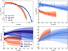 |
Fig. 1 Comparison between the median models of the MP and MR populations of Sculptor and the observed binned data from AP24. Points indicate the observed data with the bars indicating 1σ uncertainties, the solid lines the median models and the colored bands the 1σ, 2σ, and 3σ ranges. The MP and MR components are shown in blue and red, respectively, as indicated in the legend. Upper-left panel: observed surface density profiles. Upper-right panel: line-of-sight velocity dispersion profiles. Lower-left panel: radial and tangential projected velocity dispersion profiles. Only 1σ and 3σ bands are shown for simplicity. Lower-right panel: 3D velocity anisotropy profiles. |
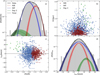 |
Fig. 2 Chemo-dynamical stellar populations of Sculptor. (a) and (d) panels: normalized metallicity and l.o.s. velocity distribution of the spectroscopically observed member stars of Sculptor alongside the median models (dashed colored lines) resulting from the fit of Sect. 4.1. Red, blue, and green indicate the MR, MP and third populations, respectively. Black shows the sum of the three components, as indicated in the legend. Bands indicate the 1σ confidence intervals. (b) and (c) panels: distribution of stars in the vlos versus [Fe/H]/R versus vlos planes. In each panel, the stars are color-coded by the population to which they have the highest probability of belonging, red for the MR, blue for the MP and green for the third population, as indicated in the legend. The systemic velocity of Sculptor is indicated with straight dashed lines. |
4.1.2 Third stellar component
We identified a third stellar component consistent with the one reported by AP24 and seen also in Tolstoy et al. (2023). Specifically, the mean metallicity of the metallicity distribution is  dex, with a dispersion
  dex. These values are in very good agreement with the ones from AP24 (
 dex and
  dex, respectively). Regarding the velocity distribution, we find a mean velocity offset with respect to Sculptor of
  and a velocity dispersion of
  , again consistent with those of AP24 (
 and
and  ).
).
The median fraction of stars expected to belong to this component is fC=0.016, which corresponds to a number of stars fC nstar=21, with a 3σ range fC=[0.006, 0.042] (corresponding to [8, 56] stars), in very good agreement with the values from AP24, a median of fC=0.017 and 3σ range fC=[0.007, 0.058]. According to the stars with larger probability of belonging to the third component than to the MP or MR ones (Eq. (13)), we find 19 stars out of the 24 initially found by AP24. Moreover, we have to consider that these DFs produce physically motivated models.
Modeling the metallicity distribution of a galaxy is challenging due to the complex chemical enrichment processes involved. As a result, Gaussian distributions may not adequately represent the metallicity distribution, potentially leading to asymmetric distributions, as commonly observed in dwarf galaxies (e.g., Kirby et al. 2011; Leaman 2012; Taibi et al. 2022). However, the case of Sculptor is somewhat peculiar. Indeed, the stars of the third population that exhibit low metallicity, representing the metal-poor tail of the MP population, also display a peculiar kinematic signature with a notably large velocity offset. This combination of low metallicity and peculiar kinematics suggests that it may represent a genuinely distinct third population. We refer the reader to AP24 for a discussion on the possible origin of this component.
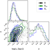 |
Fig. 3 Two-dimensional marginalized posterior distribution of rs and γ and the corresponding one-dimensional posterior distributions. The PPDs are shown when using the semi-major axis radius (black), circularized radius (green), and circular radius (blue), as indicated in the legend. |
4.2 Dark matter density profile
Fig. 3 presents the marginalized two-dimensional and onedimensional posterior distributions for the parameters γ and rs. The full marginalized posterior distributions for the remaining DM distribution parameters are shown in Fig. B.1. We first focus on the results obtained using the semi-major axis radius (represented by the black lines in Fig. 3), with a detailed discussion of other cases provided in Sect. 4.3. The PPD for γ is slightly skewed towards γ=0, suggesting a somewhat constant DM density (core) at the galaxy’s center, even though considering the entire PPD Sculptor does not have a clear constant-density region. We can also notice that rs is degenerate with γ; the larger rs, the steeper γ. The median values and 1σ confidence errors for the logarithmic inner slope and the scale radius are  and
and  kpc, more than twice the 3D half-light radius of the stellar component,
  (Muñoz et al. 2018).
In Fig. 4, we show the median cumulative DM halo mass and density profiles together with the 1σ and 3σ confidence intervals from our models, and we compare them to the ones in the literature. Our profiles are in good agreement with the ones from the literature at almost all radii. Nevertheless, as already anticipated, in the density profile we find a deficit of DM with respect to a NFW profile in the inner parts, which is more pronounced compared with other works. This could be partially because of the lower uncertainties presented in our work, the new highquality dataset and the inclusion of the discrete 2 population modeling with DFs. In Sect. 6, we compare our results with the literature ones in more detail. We also show the distributions for the stellar component, assumed to be the sum of the MR and the MP populations. To compute it, we assume the total stellar mass to be 2.3 × 10⁶ M⊙ (McConnachie 2012). It is important to note that this value is computed assuming a mass-to-light ratio of 1 M⊙/L⊙ in V-band5. The density of the stellar component decreases more rapidly than that of the DM, resulting in a DM-to-stellar mass ratio (Mhalo/M⋆) of approximately 6 at the center within 30 pc. This ratio increases to around 13 at the 3D half-light radius and reaches 154 at a distance of 2 kpc, where the farthest star in our dataset is located. Therefore, this system is highly DM dominated. However, its central regions are less DM dominated compared to previous studies.
As mentioned in the introduction, the inference of constant density cores in the DM density profile of some galaxies has motivated alternative DM models. For example, in SIDM, DM particles thermalize due to collisions in the central regions of halos, leading in some cases to the formation of constant-density cores (Sameie et al. 2020). In fuzzy DM, the DM particles are so light that they behave as waves, reaching equilibrium in a soliton configuration and forming cores (Tulin & Yu 2018). These profiles are more consistent with our findings than a pure NFW profile. However, based on our inference of the semi-major axis radius and the likelihood ratio test statistics, we can also reject a pure core (γ=0) larger than 0.7 kpc at the 99% confidence level, which is a useful constraint for these DM theories (see Chen et al. 2017).
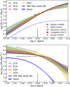 |
Fig. 4 Dark matter halo profiles inferred for Sculptor. Upper panel: Median enclosed halo mass profile together with 1σ confidence intervals (black bands). Mass indicators are shown with error bars, color-coded according to the legend. Lower panel: Dark matter halo density profile. For reference, the two inner lines indicate slopes of 1 (cusp) and 0 (core). In our dataset, there are 15 stars with log (R[kpc]) < −1.5, i.e. below the lowest radius plotted. The stellar mass profile is shown with a blue bands. The works highlighted in the legends are Z16, R19, P20 and H 20. |
4.3 Impact of different choices of radius
So far, we have compared the spherically symmetric models to the observed data by accounting for the flattened shape of Sculptor’s stellar component by labeling stars with the semi-major axis radius of the ellipse defined by the position of that star and the ellipticity of the galaxy (Eq. (1)). However, different works use different definitions (Eqs. (2) and (3)). Therefore, we have repeated the whole fitting procedure considering them.
Fig. 3 shows how the inference of Sculptor’ DM halo inner logarithm slope and scale radius are affected by these choices. The PPDs are fully consistent with each other, overlapping in the parameter space. This is reflected in the median values of γ and rs, which are  and
and  when using the circular radius, and
  and
and  for the circularized radius. Both results are in very good agreement with the inference for the semi-major axis radius, which is
  and
and  , but yielding a slightly steeper inner logarithmic slope. This result suggests that the assumption of sphericity does not significantly impact our findings, as accounting for the system’s ellipticity in different approaches or neglecting it – yields consistent results. However, this does not eliminate the need for comparisons with axisymmetric models, which can more accurately capture the effects of Sculptor’s flattening. In the literature, there have been attempts to apply axisymmetric models to real data, with methods based on Jeans modeling (Zhu et al. 2016; Hayashi et al. 2020); however, Jeans methods do not guarantee to provide physical solutions, as some of them could be generated by negative DFs, and have their own caveats. Perhaps the biggest difference between the assumptions is related to the log (ρ150) value quoted in Table 2. For the circular radius, it is
 ![Mathematical equation: $\log \left(\rho_{150}\left[M_{\odot}/\mathrm{kpc}^{-3}\right]\right)=8.14_{-0.04}^{+0.04}$](/articles/aa/full_html/2025/07/aa54826-25/aa54826-25-eq69.png) , while for the circularized radius, it is
, while for the circularized radius, it is ![Mathematical equation: $\log \left(\rho_{150}\left[M_{\odot}/\mathrm{kpc}^{-3}\right]\right)=8.07_{-0.05}^{+0.05}$](/articles/aa/full_html/2025/07/aa54826-25/aa54826-25-eq70.png) . It is also important to note that the semi-major axis radius is systematically larger than the circular and circularized ones. Therefore, the value quoted in this case is lower than in the other cases.
. It is also important to note that the semi-major axis radius is systematically larger than the circular and circularized ones. Therefore, the value quoted in this case is lower than in the other cases.
An interesting result that we obtained is that we can exclude a pure cusp in all the cases and, more generally, a NFW profile at a 3σ confidence level over a significant range of radii. This can be seen in Fig. 5, where we compare the logarithmic slope profile obtained in the three cases with the expectations for a NFW model assuming halo masses between 108 M⊙ to 1010 M⊙ consistent with the scatter in the stellar-to-halo mass relation (Sales et al. 2022) and the relation between the concentration of the NFW profile and its total mass for satellites from Moliné et al. (2023) at redshift z=0. The inconsistency with respect to a NFW profile arises not only from the value of γ but also from the steepness of the transition α. Our model predicts a median value for α of 3.6 and a 1σ confidence interval of [2.1, 5.8], whereas for a NFW α=1, meaning the transition between the two slopes occurs very rapidly. So, although we cannot confirm the existence of a core in this galaxy, we can robustly exclude a NFW DM density profile. This can possibly indicate an impact of baryonic effects in modifying the DM halo density profile of this galaxy. It is important to note that our prior on γ only allows physical models with γ ≥ 0, which could affect our inference as the prior is centered on cuspy profiles while the cored models lie on the borders (see Sect. 4.6 of Read et al. 2018). We expect that adopting a prior on γ more balanced between cored and cuspy profiles would only strengthen our conclusions.
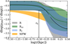 |
Fig. 5 Log-slope of the DM density profile for Sculptor. The gray, green, and blue bands show the inferred DM density according to our models for the R, Rcz and Rc cases for a 3σ confidence level. The orange band indicates the log slope profile of a pure NFW with mass and concentration as expected from cosmological consideration (see text for details), as indicated in the legend. The vertical line shows the 3-D halflight radius as reference. |
5 Test on a Sculptor-like mock
We applied our methodology to a mock dataset of R, vlos and [Fe/H] for a spherically symmetric two-component stellar system resembling Sculptor, embedding it in a cuspy spherical DM halo. The same test for a cored halo is presented in Appendix D. This experiment is meant to show that, with the quality of the dataset available, we would be able to find a cusp in Sculptor if it were there. However, as we use the same DFs to generate and analyze the mock, this test would not reveal systematic biases due to our choice of the DF. A similar experiment for a more comprehensive sets of mocks, was conducted by Read et al. (2021) using different DFs, but in the single-stellar component case.
We generated the mock dataset from the DF parameters listed in Table 3, which have been chosen so that the populations have different velocity dispersion profiles that resemble those of Sculptor. To assign metallicities to each stellar population, we use the metallicity distributions of the metal rich and metal-poor components of Sculptor reported in AP24. Following this, we extract the velocities, positions and metallicities for a set of 1339 stars. We extract them accounting for the same errors they have in our observational dataset, we do this by adding Gaussian noise to the quantities. Only the two stellar components used for the dynamical modeling are considered in this analysis, as we aim to test whether the information we have for these two components is sufficient to detect a cusp in Sculptor using our methodology.
The median and the 3σ range of the PPD for the inferred parameters after running our dynamical modeling are listed in Table 3. We can see that the inferred parameters are in very good agreement with the true values, which are very close to the median and always within 3σ. The DM density and anisotropy profiles of the mock dataset and the ones resulting from the fitting procedure are shown in Fig. 6. We recovered with high precision the true profiles, within the 1σ bands. Therefore, we conclude that, at least in this ideal case where we built our mock dataset with the same DF we are using to analyze it, our model is capable of recovering the cusp in a dSph-like galaxy with a dataset similar to the one of Sculptor. Furthermore, it can independently constrain the anisotropy profile of both populations. However, the uncertainties on the inner logarithm slope do not allow one to discard a cored DM distribution within 3σ.
When analyzing a cored halo mock dataset (see Appendix D), the inferred parameters also show very good agreement; the true values are always very close to the medians and lie within 3σ. Even though the inference of γ is consistent with 0 only within 3σ, it is something to expect, as we only allowed models with γ > 0, but the PPD is completely skewed towards 0. This same effect could explain why rs is also in the 3σ border, as it is degenerated with γ. Overall, the inferred profiles also match the true ones with high precision.
We also analyzed the cusped mock galaxy assuming that there is only one single population, resembling the observational scenario where the two independent populations are not considered. The results of the fit are listed in Table 3. The inferred parameters are offset from the true ones and not within 1σ. Notably, now we infer a distribution much closer to a core, but with large uncertainties and consistent with a cusp within 3σ.
Inference on the free parameters of the models for the cuspy mock.
6 Comparison with the literature
Here, we compare our results with those from the literature. Specifically, in Sect. 6.1, we compare the mass estimators used to compute the total mass within a given radius. In Sect. 6.2, we present the DM density profiles reported in previous works and compare them with ours.
6.1 Mass estimators
In the literature, many authors have managed to constrain the dynamical mass enclosed within a certain characteristic radius by using mass estimators of the form
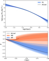 |
Fig. 6 Upper panel: dark matter density profile of the mock galaxy. In black, we show the underlying one, the median of the predicted profile is shown with a solid blue line and the blue bands indicate the 1σ, 2σ, and 3σ confidence intervals. Lower panel: Velocity anisotropy profile for the MP and MR stellar components. As solid lines, we show the values for the underlying model and in bands the best-fit for the MR and the MP component, indicating the 1σ, 2σ, and 3σ confidence intervals. The solid black line corresponding to the MR component become gray in the region in which we do not produce stars that belong to that component. |
 (14)
(14)
In the above equation, Mdyn(< xRh) is the dynamical mass within x times the projected half-light radius Rh (other formulations express it as a function of the 3-D half-light radius), K is a dimensionless constant, G the gravitational constant, and ⟨σl.o.s.⟩ the mean l.o.s. velocity dispersion of the stellar system. Different studies have derived different values for K and x, depending on their different assumptions. In the cumulative mass profile shown in the top panel of Fig. 4 one can compare our results with the ones obtained by using the estimators derived by Walker et al. (2009); Wolf et al. (2010); Amorisco & Evans (2012); Campbell et al. (2017); Errani et al. (2018). The estimators that provide a value of the enclosed mass beyond the projected half-light radius are in very good agreement with our results (Amorisco & Evans 2012; Campbell et al. 2017; Errani et al. 2018). On the other hand, estimators that provide a value of enclosed mass around the halflight radius (Walker et al. 2009; Wolf et al. 2010) deviate more from our findings.
In general, simple mass estimators also show lower errors than the dynamical modeling methods when computed via error propagation. However, this might be a problem of calibration, as different works testing mass estimators in simulations have shown that there is larger scatter in the results (González-Samaniego et al. 2017; Sarrato et al., in prep.) than uncertainties computed here by applying error propagation of Mdyn(< nRh) and Rh uncertainties.
6.2 Dynamical modeling
There are different techniques to estimate the DM density profile of a pressure-supported system (see, e.g., Battaglia & Nipoti 2022). Those that directly solve the Jeans equation are known as Jeans modeling (Read et al. 2019; Hayashi et al. 2020; Wardana et al. 2025, for example). Another method is Schwarzschild orbit-superposition modeling (Schwarzschild 1979), which is based on representing the target galaxy as the superposition of orbits (Breddels et al. 2013; Breddels & Helmi 2013). Each orbit type is assigned a weight that is optimized to match the observed data. Distribution function modeling techniques, such as the one used here, model the target phase-space distribution directly assuming an analytic form of the DF. This latter method has the advantage that all observables can be directly computed from the DF. These three methods have been applied to Sculptor in several works, and here we conduct a comprehensive comparison with all existing studies that have inferred the DM density of Sculptor. Table 4 lists all the works and their main characteristics and assumptions. In general, our results are consistent with the existing literature, even though the quoted uncertainties in the different methods are large. Overall, most of the studies favor a core over a cusp for Sculptor. Only R19 and E23 clearly favor cuspy solutions. Given the many differences between studies in terms of datasets, methods, and assumptions, it is challenging to identify the factors driving the discrepancies in the results. Nevertheless, in the following, we briefly describe each of them and compare their results with ours.
B08: in this study, the authors performed Jeans modeling, fitting both populations simultaneously using binned data and the semi-major axis radius to label the stars. The authors assume that the stellar populations are tracers that follow a Plummer density profile for the MP component and a Sersic profile for the MR. For the DM component, the authors test two different models, a NFW and a pseudo-isothermal sphere, and two different velocity anisotropy profiles, an Osipkov-Merritt (OM) (Osipkov 1979; Merritt 1985) and constant profiles, finding that the OM one was preferred to the others. They compare cuspy and cored models based on χ2 values, finding that the cored ones reproduce the data better than the cusped. In particular, the NFW model predicts larger velocity dispersion for the MR component than the observed one. Their best-fit model has a core of 0.5 kpc, in marginal agreement with the scale radius we find,  . We note that the scale radius of our profile is degenerate with the value of γ, see Fig. B.1. It is remarkable that, despite the differences in the methodology and dataset, the results are highly consistent.
W11: in this work, the authors used an estimator for the inner slope of the DM profile, which is a function of the ratios between the velocity dispersion and the half-light radii of two stellar populations. They show that this estimator is biased towards predicting cuspy profiles by applying it to a mock sample. Their analysis assumes a Gaussian velocity distribution, with the spatial distribution modeled by a Plummer profile. Data from Walker et al. (2009) is used, and incompleteness is taken into account. They excluded NFW or steeper profiles for Sculptor with a significance level of 99.8% when using circular radii and of 93.9% when using semi-major axis radii. Interestingly, they found more evidence of a core when using circular radii, contrary to our results. However, both results are in agreement with our inference, and this could be just an effect of the different datasets used.
AE12: in this work, the authors used energy and angular momentum based DFs to model the data from Battaglia et al. (2008), using semi-major axis radii. In particular, they used Michie-king DFs (King 1962; Michie 1963), assuming a positive-defined velocity anisotropy that can vary with the radius. They fit both populations simultaneously, treating them as independent tracers of the underlying potential, with the assumption that the stars are just dynamical tracers. For the DM component, they compared only two different models, a NFW and a cored NFW profile. The model selection is based on χ2 values. They found that a cored distribution fit the data better compared to a cusped configuration. The scale radius for the cored model is 0.36 kpc, slightly smaller than ours, but completely consistent given the errors and the degeneracy with γ.
B13a & B13b: in these works, the authors performed Schwarzschild modeling to fit the second and fourth velocity moments. They combined the data from both Battaglia et al. (2008) and Walker et al. (2009), and they fit binned data using circular radius (Eq. (2)) to label the stars. They assume that all the stars belong to a single population and are tracers of the underlying potential. In B13a, the inner slope of their DM potential is a free parameter, while in B13b the authors test different DM density profiles and compared them according to χ2 values. In Schwarzchild models, the velocity anisotropy is an output, so it is non-parametric and can vary with radius. In B13a, the authors find that the inner slope of the DM density profile remains unconstrained between 0 and 1.2, excluding very steep profiles γ > 1.5. However, they still find the maximum of their PPD at γ=0, as in our inference. In B13b the authors find that, according to χ2 values, a cusp is preferred. However, the evidence is “barely worth mentioning” according to the Jeffrey’s scale. In contrast with our results and with the measurements of Massari et al. (2018), they found that the overall population of Sculptor shows tangential orbits (β < 0).
R14: in this work, the authors performed spherically symmetric Jeans modeling using the virial shape parameter, which provide additional constraints on anisotropy through higherorder virial equations. They use the data from Walker et al. (2009) and bin them using circular radius. They assume that all the stars belong to a single population and model the stellar component with a Plummer model. For the DM, they explore two different approaches. First, they fix the profile to a NFW profile (cusped) and a Burkert profile (cored) (Burkert 1995). Second, they use a Zhao profile (Zhao 1996) with a free inner slope. The velocity anisotropy profile can vary freely with the radius. For the fixed DM density profile case, they found that, according to χ2, a cored DM profile fits the data better than the NFW one. However, when they let the inner and outer slopes free, there is a lot of degeneracy. Both a cusp with an outer slope >2.5 or a core with an outer slope of around 2 fit the data equally well. This could hint that comparing two DM density profiles according to the evidence of two different models, could be leading to false constrained results, and once should instead use a more general model. In contrast with this work we find a core with an outer slope larger than 2.5, but the differences could arise from the different datasets, models and method used.
Z16: in this work, the authors fit the data using axisymmetric Jeans modeling and including rotation in their models. They fit individual stars from the dataset of Walker et al. (2009). The study fits the two populations independently, using the metallicity to distinguish populations. The stellar density profiles are computed assuming a Gaussian expansion, and the stars are considered tracers. For the DM density profile, they use a generalized NFW distribution with a free inner slope. The velocity distribution is approximated as Gaussian with added rotation and a radially constant anisotropy. They find an inner slope of 0.5 ± 0.3(1σ). The PPD is slightly bimodal, with peaks at around 0.25 and 0.75, but in general the result is consistent with ours.
S17: this study uses dynamical modeling with energy and angular momentum DFs for the stars. They use the data from Battaglia et al. (2008) binned in semi-major axis radius and Walker et al. (2009) binned in circular radius, independently. They use two different potentials, a NFW profile (cusped) and a Burkert profile (cored). Two populations are fitted simultaneously, with a free anisotropy parameter allowing for a transition from radial to tangential orbits both at the center and at larger distances. The χ2 comparison shows a slightly better fit for a cored profile when analyzing the data from Battaglia et al. (2008). However, when analyzing the data from Walker et al. (2009) the preferred model is cusped.
K19: in this work, the authors performed Jeans modeling. They use binned data from Walker et al. (2009), assuming only one population. They assume a Plummer profile for the stellar component. For the DM component, they try two different models, a NFW and a cored isothermal profile (Kaplinghat et al. 2016). The velocity anisotropy can vary with the radius, allowing both radial and tangential orbits. They find moderate to strong evidence of the cored models being preferred according to the scale of Bauldry (2015).
R19: using the software GravSphere, the authors solved the Jeans equations by fitting binned data with two virial shape parameters. They use binned data from Walker et al. (2009). The stellar density is modeled using a sum of three Plummer spheres. The DM distribution follows a cored NFW profile with flexible γ. Anisotropy is free, and stars are treated as tracers. The authors find a logarithmic inner slope of  , marginally consistent with our inference. They also find a value of
  , while we infer a lower density
  . The key differences between the works are that we used discrete rather than binned data, we used both populations as independent tracers of the same potential, and we conducted DF-based modeling, while they used Jeans modeling.
H20: in this work, the authors applied axisymmetric Jeans modeling. They use the data from Walker et al. (2009), fitting individual stars and assuming only one population. For the stellar component, they fit an axisymmetric Plummer profile and assume that the stars are tracers. For the DM density, they use a double power-law density profile. They find a value of the logarithmic inner slope of  , which is within 1σ with our results.
E23: the authors used a probabilistic deep learning approach, trained on velocity maps of pressure supported galaxies from NIHAO simulations. This technique applied is applied to Walker et al. (2009) data, and it predicts a cusp for Sculptor. This suggests that cusped galaxies in these simulations resemble the observed characteristics of Sculptor better than those with cored profiles. However, it remains to be proven if these simulations accurately represent observed galaxies in this mass regime.
Literature results for the logarithm inner slope of the DM halo of Sculptor.
7 Discussion
In this section, we discuss the main results of this work. In Sect. 7.1, we review the implications of Sculptor having a DM halo density profile deviating from a pure-NFW in the context of feebdback-induced effects. In Sect. 7.2, we analyze how suitable Sculptor is as a candidate target for DM detection.
7.1 Sculptor’s DM halo properties accounting for stellar feedback
According to the studies in the literature with the most efficient transformations of cusps into core due to supernovae feedback, one would expect cores to be formed around M⋆/Mhalo=10−2 (Di Cintio et al. 2014b; Oñorbe et al. 2015) and cusps being preserved around M⋆/Mhalo=10−4. Assuming that LG dwarf galaxies follow the mass-dependent density profile proposed in Di Cintio et al. (2014a), Brook & Di Cintio (2015) estimate γ ∼ 0.6, in line with our determination. The possibility that Sculptor’s DM halo density profile has been affected by supernovae feedback is also aligned with the work by Bermejo-Climent et al. (2018), who, on the basis of the estimated amount of energy deposited by supernovae feedback based on SFHs from deep CMD predict that Sculptor and Fornax are the Milky Way dSphs most likely to host cored DM haloes.
Nonetheless, there is still significant uncertainty in the predictions. For example, some higher resolution simulations show that approximately constant density cores with core sizes of the order of the stellar half-light radius (e.g., Read et al. 2016) or up to 0.5−1 kpc (Oñorbe et al. 2015) can form even for M⋆/Mhalo ∼ 10−4; although, a condition for this to happen is substantial latetime star formation. In particular, recently, Muni et al. (2025) have found the central DM density (quantified through ρ150) to correlate strongly with (and to be a decreasing function of) the ratio between the stellar mass formed post- and before reionization. Observationally, it is hard to quantify the amount of stellar mass formed before and after re-ionization; an handier indicator could be the times in which 50 and 90 percent of the stellar mass formed. In any case, the latest results in the literature indicate that most star formation in Sculptor occurred in the first Gyr of evolution, with the stellar mass essentially in place at a lookback time of 10−11 Gyr (e.g., Bettinelli et al. 2019) or extending out to 4-6 Gyr ago but still with the great majority of star formation occurring early on, out to 8−9 Gyr ago (e.g., de Boer et al. 2012; Savino et al. 2018). In addition, our dynamical analysis suggests an almost constant inner slope out to a radius about twice the half-light radius. These are all interesting constraints that simulations can aim at reproducing.
Since, as highlighted in Muni et al. (2025), the potential to overcome for core creation is not that of the whole halo but rather that of the concentrated central regions, in Table 2 we also provide the DM mass within the half-light radius and 2 kpc.
7.2 Sculptor as a target for indirect DM searches
Dwarf galaxies are among the best targets to look for high energy emission due to DM particles annihilation or decay (Albert et al. 2020; Hu et al. 2024). This is because they are very DM dominated, close enough and with a size in the sky so that they can be almost fully observed with the aperture of the telescopes usually used for this task. Once the DM density profile of a dSph is known, it is straightforward to predict the gamma flux due to emission from annihilation or decay of DM particles as a function of the aperture observed. The γ-ray flux is proportional to the so-called J (annihilation) and D (decay) factors. They can be computed as
 (15)
(15)
and
 (16)
(16)
where θ=R/d is the angular distance from the center of the galaxy, z indicates the l.o.s. direction, d is the distance to the galaxy, and ρDM is the DM density. In Table 2 we provide the J – and D – factors computed for θ=0.5°, for the case of semimajor axis radius. The factors computed by H 20 are larger than ours, but within 2σ, because of the denser profile at the center. Interestingly, compared with Geringer-Sameth et al. (2015), we find a lower value for J(0.5°) but a considerably larger one for D(0.5°), this is explained by different shapes in the DM density profile. Very similar results were already quoted with these models in (Nipoti et al. 2024), the very minor differences are because of the use of a slightly different photometric center for Sculptor.
8 Conclusions
In this work, we have used dynamical models based on DFs depending on actions to fit state-of-the-art measurements of the kinematics and metallicities of Sculptor member stars with the aim of inferring the DM density distribution of the galaxy. In these models we fit discrete data in the form of individual l.o.s. velocities, metallicities, and positions. We relied on a full Bayesian framework to constrain the PPD of all model parameters. We identified the two main stellar populations of this galaxy, which have a median metallicity of around [Fe/H]=−1.4 and −2.0, and we confirmed the presence of a third population, in agreement with previous works. Probabilities of membership were computed based on these models. In the following, we report our main results:
We find a ratio of dark-to-stellar mass of
 , and
, and  at 0.03 kpc, 0.32 kpc(rh), and 2 kpc, with 2 kpc being our outermost measured point. The last value sets an upper limit of M⋆/Mhalo around 5−8 × 10⁻³, providing a constraint for abundance matching relations on small galactic scales and for models of stellar feedback-induced transformations of initially cuspy DM haloes;
We find that the DM density profile in the inner region of the galaxy has an inner logarithmic slope of
 and a PPD shifted towards zero. This slope extends to
  , a value that exceeds the half-light radius of the stellar component rh. The DM density profile also exhibits a rather steep transition between the inner and outer slopes. Such a profile in a faint dwarf galaxy with a short SFH as that of Sculptor can place constraints on DM models or feedback implementations in simulations;
We confirmed that the third stellar component found by AP24 did not arise due to the limitations of the velocity and position distributions used in that work. It still remains to be tested whether a more flexible metallicity distribution that considers the inclusion of tails would remove the existence of this population but still reproduce its velocity distribution shifted from Sculptor’s systemic velocity;
We tested the dynamical modeling technique presented here on two mock galaxies, one with a cuspy DM halo and one with a DM halo exhibiting a constant density core of a size similar to Sculptor’s half-light radius. These mock galaxies resemble the characteristics of Sculptor stellar populations and the spectroscopic dataset being analyzed. We find that the multi-population fitting is able to retrieve the presence of a cusp within 1σ. Hence, if a cusp were present, we would have been able to detect it. Similarly, the cored DM density profile is also well recovered by our methodology. Interestingly, we find that when treating the stellar component as a single population, we are not able to recover the cusped DM distribution within 1σ and barely within 3σ;
We also analyzed the effect of adopting different choices for labeling the radius of the stars (semi-major axis radius, circularized, and circular) to compare with the radius in the spherically symmetric models. We find that results are consistent with each other. Moreover, in all cases, the logarithmic slope of the DM halo density profile appears to be incompatible with an NFW profile at a 3 σ confidence level within the radial range below the half-light radius of the stellar component;
Our models predict a velocity anisotropy parameter profile that starts at β=0 in the center and gradually becomes radially biased for both the MR and MP components. Additionally, we predict that the projected radial and tangential velocity dispersions on the plane of the sky should increase and decrease with radius, respectively, in both populations.
Regarding our interpretation of DM density profiles of dwarf galaxies in the context of the nature of DM versus the impact of baryonic effects, a systematic study of a sample of dwarf galaxies with high-quality data and probing a range of stellar masses and SFHs would offer an invaluable opportunity to accurately characterize the relationships between DM density profiles and the properties of their stellar populations and provide constraints to the still uncertain model predictions. Ideally, one would extend the analysis to as large radii as possible to alleviate uncertainties in the stellar-to-halo mass relation. In the close future, wide field of view multi-object spectrographs such as WEAVE (Dalton et al. 2012), 4MOST (Skúladóttir et al. 2023), and PFS (Takada et al. 2014) will provide reliable l.o.s. velocities and metallicities for more as well as new members in the central regions and outskirts of Milky Way dSphs in a very efficient manner.
A higher precision in the determination of the DM halo slope at different radii and as close to the center as possible is something to be sought in order to exclude more of the parameter space of possible DM halo models. The inclusion of projected tangential velocities of individual stars from upcoming proper motion measurements, such as the ones already presented for some dwarfs (e.g., Draco from HST measurements (Vitral et al. 2024)) and upcoming measurements from Gaia DR5 and the Nancy Roman/WFIRST telescope (Spergel et al. 2015), will offer a valuable opportunity in this respect, particularly if they are available for of the order of 1000 stars per galaxy (e.g., Read et al. 2021). The methodology presented here has already been adapted to incorporate the proper motions of stars without a significant increase in computational time (e.g., Della Croce et al. 2024).
Acknowledgements
J. M. Arroyo acknowledges support from the Agencia Estatal de Investigación del Ministerio de Ciencia en Innovación (AEI-MICIN) and the European Social Fund (ESF+) under grant PRE2021-100638. J. M. Arroyo, G. Battaglia, G. Thomas acknowledge support from the Agencia Estatal de Investigación del Ministerio de Ciencia, Innovación y Universidades (MCIU/AEI) under grant “En La Frontera De La Arqueología Galáctica: Evolución De La Materia Luminosa Y Oscura De La Vía Láctea Y Las Galaxias Enanas Del Grupo Local En La Era De Gaia. (FOGALERA)”, the European Regional Development Fund (ERDF) with reference PID2023-150319NB-C21 and PID2020-118778GB-I00 and the AEI under grant number CEX2019-000920-S. E. Vasiliev acknowledges support from an STFC Ernest Rutherford fellowship (ST/X004066/1) and from the Severo Ochoa Centres of Excellence programme (CEX2019-000920-S). This paper is supported by the Italian Research Center on High Performance Computing Big Data and Quantum Computing (ICSC), project funded by European Union – NextGenerationEU and National Recovery and Resilience Plan (NRRP) – Mission 4 Component 2 within the activities of Spoke 3 (Astrophysics and Cosmos Observations). J.M. Arroyo-Polonio, G. Battaglia and G. Thomas acknowledge funding received from the European Union through the grant “UNDARK” of the Widening participation and spreading excellence programme (project number 101159929). The authors acknowledge the referee for the constructive report, which enhanced the quality of the manuscript.
Appendix A Markov chain Monte Carlo
We run our model with three populations (25 free parameters) using semi-major axis radius, circularized radius and circular radius. By doing so, we characterize the variations on the DM properties produced by this choice. We use a Markov chain Monte Carlo (MCMC) method and rely on the EMCEE package (Foreman-Mackey et al. 2013), a python implementation of the affine invariant MCMC ensemble sampler (Goodman & Weare 2010). For these runs we use 100 initial walkers. We also analyzed the galaxy using only the MR and MP populations, see Appendix C. In these cases, we have 10 free parameters, 5 for the stellar component and 5 for the DM density. For those cases, we used 60 walkers. Finally, we analyzed a cusped mock galaxy. In this case, we considered only a 2 populations model (20 free parameters) and a single population one (10 free parameters). We used 80 and 40 walkers, respectively. In all the cases the runs were long enough to obtain at least, 1000 steps after the burn-in for the 90 walkers, which we checked and ensures stability in the inference of the parameters. The specifications of all the runs can be seen in Table A.1. The median is computed as the 50th percentile of the PPD and the 1σ and 3σ confidence intervals are defined by the [16th, 84th] and the [0.15th. and the 99.85th] percentiles.
We show all the specifications for the EMCEE runs. Column 1 lists the models; Col. 2 shows the number of free parameters; Col. 3 indicates the final number of walkers used; Col. 4 lists number of steps; Col. 5 presents the number of burning steps; and finally, Col. 6 lists the value of the thinning. We checked that there are enough steps after the burning to ensure convergence and that the value of the thinning do not have a strong impact on the inference.
Appendix B Bayesian inference
In this section, we show the inference of all the 25 free parameters for the semi-major axis radius case split in different groups. In Fig. B.1 we show the inference for the DM, in Fig. B.2 for the MP component, in Fig. B.3 for the MR component and in Fig. B.4 for the third population.
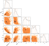 |
Fig. B.1 Corner-plot showing the PPD for the free parameters of the DM halo. The first parameter is the total mass MDM in M⊙, the second the scale-radius rs in kpc and the third one the steepness of the transition α between the outer slope (fourth parameter, η) and the inner slope (fifth parameter, γ). |
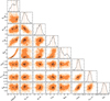 |
Fig. B.2 Corner-plot showing PPD of the free parameters of the MP component. The eight parameters shown |

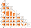 |
Fig. B.3 Corner-plot showing PPD of the free parameters of the MR component. The eight parameters shown |

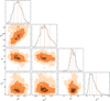 |
Fig. B.4 Corner-plot showing PPD of the free parameters of the third stellar component. The four parameters shown |

Appendix C Inference with individual populations
In this section, we compute the DM density profile of Sculptor using only the MR and MP populations independently. Assign membership to each star to the population it has the highest probability to belong, accourding to the probabilities of membership from AP24. In Fig. C.1 we show the results of the analysis. The results are consistent across all the range except in the outer part for the MR component. This could be explained by the lack of MR stars in that region. The main difference is that the profiles are considerably less constrained, and they have larger errors. As a result, the inference on γ of individual populations fitting is in marginal agreement with both, cusped and cored profiles. For only the MR population the median of γ is 0.50, while the 1σ and 3σ intervals are [0.19, 0.91] and [0.00, 1.51]. While for only the MP population the median of γ is 0.45, while the 1σ and 3σ intervals are [0.12, 0.94] and [0.00, 1.34] This highlights the importance of having two independent tracers of the potential and the statistics necessary to constrain the inner slopes.
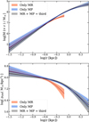 |
Fig. C.1 Upper panel: Cumulative DM halo mass distribution. Lower panel: DM halo density distribution. In different colors we show the inferred DM density profile obtained by using the two independent populations as tracers (black), only the MR population (red) and only the MP population (blue), as indicated in the legend. |
Appendix D Test on a Sculptor-like mock with a cored DM halo
Here, we repeat the experiment we described on Sect. 5, but using a cored DM halo. The core has a scale radius of 0.32 kpc, similar to the half-light radius of the stellar component in Sculptor (Muñoz et al. 2018). A comparison between the inferred parameters and their true values is presented in Table D.1, while the resulting DM density and β profiles are shown in Fig. D.1. Both the inferred parameters and the profiles are in very good agreement with the underlying ones, there are some minor tensions in rs and γ discussed in Sect. 5.
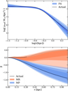 |
Fig. D.1 Upper panel: Dark matter density profile recovered for the cored mock galaxy. In black, we show the underlying one, the median of the predicted profile is shown with a solid blue line and the blue bands indicate the 1σ, 2σ and 3σ confidence intervals. Lower panel: Velocity anisotropy profile for the MP and MR stellar components. As solid lines, we show the values for the underlying model and in bands the best-fit for the MR and the MP component, indicating the 1σ, 2σ and 3σ confidence intervals. The solid black line corresponding to the MR component become gray in the region in which we do not produce stars that belong to that component. |
Inference on models free parameters for the cored mock.
References
- Albert, A., Alfaro, R., Alvarez, C., et al. 2020, Phys. Rev. D, 101, 103001 [Google Scholar]
- Amorisco, N. C., & Evans, N. W. 2012, MNRAS, 419, 184 [NASA ADS] [CrossRef] [Google Scholar]
- Aparicio, A., Carrera, R., & Martínez-Delgado, D., 2001, AJ, 122, 2524 [NASA ADS] [CrossRef] [Google Scholar]
- Arroyo-Polonio, J. M., Battaglia, G., Thomas, G. F., et al. 2024, A&A, 692, A195 [NASA ADS] [CrossRef] [EDP Sciences] [Google Scholar]
- Battaglia, G., & Nipoti, C., 2022, Nat. Astron., 6, 659 [NASA ADS] [CrossRef] [Google Scholar]
- Battaglia, G., Helmi, A., Tolstoy, E., et al. 2008, ApJ, 681, L13 [NASA ADS] [CrossRef] [Google Scholar]
- Battaglia, G., Taibi, S., Thomas, G. F., & Fritz, T. K., 2022, A&A, 657, A54 [NASA ADS] [CrossRef] [EDP Sciences] [Google Scholar]
- Bauldry, S., 2015, in International Encyclopedia of the Social & Behavioral Sciences, 2nd edn., ed. J. D. Wright (Oxford: Elsevier), 615 [Google Scholar]
- Bermejo-Climent, J. R., Battaglia, G., Gallart, C., et al. 2018, MNRAS, 479, 1514 [NASA ADS] [CrossRef] [Google Scholar]
- Bettinelli, M., Hidalgo, S. L., Cassisi, S., et al. 2019, MNRAS, 487, 5862 [NASA ADS] [CrossRef] [Google Scholar]
- Binney, J., 2014, MNRAS, 440, 787 [Google Scholar]
- Binney, J., & Mamon, G. A., 1982, MNRAS, 200, 361 [Google Scholar]
- Binney, J., & Piffl, T., 2015, MNRAS, 454, 3653 [NASA ADS] [CrossRef] [Google Scholar]
- Binney, J., & Vasiliev, E., 2023, MNRAS, 520, 1832 [NASA ADS] [CrossRef] [Google Scholar]
- Breddels, M. A., & Helmi, A., 2013, A&A, 558, A35 [NASA ADS] [CrossRef] [EDP Sciences] [Google Scholar]
- Breddels, M. A., Helmi, A., van den Bosch, R. C. E., van de Ven, G., & Battaglia, G., 2013, MNRAS, 433, 3173 [NASA ADS] [CrossRef] [Google Scholar]
- Brook, C. B., & Di Cintio, A., 2015, MNRAS, 450, 3920 [CrossRef] [Google Scholar]
- Bullock, J. S., & Boylan-Kolchin, M., 2017, ARA&A, 55, 343 [Google Scholar]
- Burkert, A., 1995, ApJ, 447, L25 [NASA ADS] [Google Scholar]
- Campbell, D. J. R., Frenk, C. S., Jenkins, A., et al. 2017, MNRAS, 469, 2335 [Google Scholar]
- Carlson, E. D., Machacek, M. E., & Hall, L. J., 1992, ApJ, 398, 43 [CrossRef] [Google Scholar]
- Carrera, R., Pancino, E., Gallart, C., & del Pino, A., 2013, MNRAS, 434, 1681 [NASA ADS] [CrossRef] [Google Scholar]
- Chen, S.-R., Schive, H.-Y., & Chiueh, T., 2017, MNRAS, 468, 1338 [NASA ADS] [CrossRef] [Google Scholar]
- Dalton, G., Trager, S. C., Abrams, D. C., et al. 2012, SPIE Conf. Ser., 8446, 84460P [Google Scholar]
- de Blok, W. J. G., Walter, F., Brinks, E., et al. 2008, AJ, 136, 2648 [NASA ADS] [CrossRef] [Google Scholar]
- de Boer, T. J. L., Tolstoy, E., Hill, V., et al. 2012, A&A, 544, A73 [NASA ADS] [CrossRef] [EDP Sciences] [Google Scholar]
- de los Reyes, M. A. C., Kirby, E. N., Ji, A. P., & Nuñez, E. H. 2022, ApJ, 925, 66 [NASA ADS] [CrossRef] [Google Scholar]
- del Pino, A., Libralato, M., van der Marel, R. P., et al. 2022, ApJ, 933, 76 [NASA ADS] [CrossRef] [Google Scholar]
- Della Croce, A., Pascale, R., Giunchi, E., et al. 2024, A&A, 682, A22 [NASA ADS] [CrossRef] [EDP Sciences] [Google Scholar]
- Di Cintio, A., Brook, C. B., Dutton, A. A., et al. 2014a, MNRAS, 441, 2986 [Google Scholar]
- Di Cintio, A., Brook, C. B., Macciò, A. V., et al. 2014b, MNRAS, 437, 415 [Google Scholar]
- El-Zant, A., Shlosman, I., & Hoffman, Y., 2001, ApJ, 560, 636 [NASA ADS] [CrossRef] [Google Scholar]
- Errani, R., Peñarrubia, J., & Walker, M. G., 2018, MNRAS, 481, 5073 [CrossRef] [Google Scholar]
- Expósito-Márquez, J., Brook, C. B., Huertas-Company, M., et al. 2023, MNRAS, 519, 4384 [CrossRef] [Google Scholar]
- Foreman-Mackey, D., Hogg, D. W., Lang, D., & Goodman, J., 2013, PASP, 125, 306 [Google Scholar]
- Gallart, C., Monelli, M., Mayer, L., et al. 2015, ApJ, 811, L18 [NASA ADS] [CrossRef] [Google Scholar]
- Gentile, G., Salucci, P., Klein, U., Vergani, D., & Kalberla, P., 2004, MNRAS, 351, 903 [Google Scholar]
- Geringer-Sameth, A., Koushiappas, S. M., & Walker, M., 2015, ApJ, 801, 74 [NASA ADS] [CrossRef] [Google Scholar]
- González-Samaniego, A., Bullock, J. S., Boylan-Kolchin, M., et al. 2017, MNRAS, 472, 4786 [CrossRef] [Google Scholar]
- Goodman, J., & Weare, J., 2010, Commun. Appl. Math. Computat. Sci., 5, 65 [Google Scholar]
- Hayashi, K., Chiba, M., & Ishiyama, T., 2020, ApJ, 904, 45 [NASA ADS] [CrossRef] [Google Scholar]
- Hopkins, P. F., Kereš, D., Oñorbe, J., et al. 2014, MNRAS, 445, 581 [NASA ADS] [CrossRef] [Google Scholar]
- Hu, W., Barkana, R., & Gruzinov, A., 2000, Phys. Rev. Lett., 85, 1158 [NASA ADS] [CrossRef] [Google Scholar]
- Hu, X.-S., Zhu, B.-Y., Liu, T.-C., & Liang, Y.-F. 2024, Phys. Rev. D, 109, 063036 [Google Scholar]
- Iorio, G., Nipoti, C., Battaglia, G., & Sollima, A., 2019, MNRAS, 487, 5692 [CrossRef] [Google Scholar]
- Kaplinghat, M., Tulin, S., & Yu, H.-B. 2016, Phys. Rev. Lett., 116, 041302 [NASA ADS] [CrossRef] [Google Scholar]
- Kaplinghat, M., Valli, M., & Yu, H.-B. 2019, MNRAS, 490, 231 [NASA ADS] [CrossRef] [Google Scholar]
- King, I., 1962, AJ, 67, 471 [Google Scholar]
- Kirby, E. N., Lanfranchi, G. A., Simon, J. D., Cohen, J. G., & Guhathakurta, P., 2011, ApJ, 727, 78 [Google Scholar]
- Leaman, R., 2012, AJ, 144, 183 [NASA ADS] [CrossRef] [Google Scholar]
- Leung, G. Y. C., Leaman, R., Battaglia, G., et al. 2021, MNRAS, 500, 410 [Google Scholar]
- Martínez-García, A. M., del Pino, A., & Aparicio, A., 2023, MNRAS, 518, 3083 [Google Scholar]
- Martínez-Vázquez, C. E., Monelli, M., Bono, G., et al. 2015, MNRAS, 454, 1509 [Google Scholar]
- Mashchenko, S., Couchman, H. M. P., & Wadsley, J., 2006, Nature, 442, 539 [NASA ADS] [CrossRef] [Google Scholar]
- Massari, D., Breddels, M. A., Helmi, A., et al. 2018, Nat. Astron., 2, 156 [Google Scholar]
- McConnachie, A. W., 2012, AJ, 144, 4 [Google Scholar]
- Merritt, D., 1985, AJ, 90, 1027 [Google Scholar]
- Michie, R. W., 1963, MNRAS, 125, 127 [Google Scholar]
- Moliné, Á., Sánchez-Conde, M. A., Aguirre-Santaella, A.,, et al. 2023, MNRAS, 518, 157 [Google Scholar]
- Muñoz, R. R., Côté, P., Santana, F. A., et al. 2018, ApJ, 860, 66 [CrossRef] [Google Scholar]
- Muni, C., Pontzen, A., Read, J. I., et al. 2025, MNRAS, 536, 314 [Google Scholar]
- Navarro, J. F., Frenk, C. S., & White, S. D. M., 1997, ApJ, 490, 493 [Google Scholar]
- Nipoti, C., & Binney, J., 2015, MNRAS, 446, 1820 [NASA ADS] [CrossRef] [Google Scholar]
- Nipoti, C., Pascale, R., & Arroyo-Polonio, J. M., 2024, arXiv e-prints, [arXiv:2411.05084] [Google Scholar]
- Oñorbe, J., Boylan-Kolchin, M., Bullock, J. S., et al. 2015, MNRAS, 454, 2092 [CrossRef] [Google Scholar]
- Osipkov, L. P., 1979, Pisma Astron. Z., 5, 77 [Google Scholar]
- Pace, A. B., Kaplinghat, M., Kirby, E., et al. 2020, MNRAS, 495, 3022 [NASA ADS] [CrossRef] [Google Scholar]
- Pascale, R., 2020, PhD thesis, alma [Google Scholar]
- Pascale, R., Posti, L., Nipoti, C., & Binney, J., 2018, MNRAS, 480, 927 [Google Scholar]
- Pascale, R., Binney, J., Nipoti, C., & Posti, L., 2019, MNRAS, 488, 2423 [NASA ADS] [CrossRef] [Google Scholar]
- Pascale, R., Calura, F., Lupi, A., et al. 2023, MNRAS, 526, 1428 [NASA ADS] [CrossRef] [Google Scholar]
- Pascale, R., Nipoti, C., Calura, F., & Croce, A. D., 2025, Leo I: the classical dwarf spheroidal galaxy with the highest dark-matter density [Google Scholar]
- Pasquini, L., Avila, G., Blecha, A., et al. 2002, The Messenger, 110, 1 [Google Scholar]
- Pietrinferni, A., Cassisi, S., Salaris, M., & Hidalgo, S., 2013, A&A, 558, A46 [NASA ADS] [CrossRef] [EDP Sciences] [Google Scholar]
- Plummer, H. C., 1911, MNRAS, 71, 460 [Google Scholar]
- Pontzen, A., & Governato, F., 2014, Nature, 506, 171 [NASA ADS] [CrossRef] [Google Scholar]
- Posti, L., Binney, J., Nipoti, C., & Ciotti, L., 2015, MNRAS, 447, 3060 [Google Scholar]
- Read, J. I., Agertz, O., & Collins, M. L. M., 2016, MNRAS, 459, 2573 [NASA ADS] [CrossRef] [Google Scholar]
- Read, J. I., Walker, M. G., & Steger, P., 2018, MNRAS, 481, 860 [NASA ADS] [CrossRef] [Google Scholar]
- Read, J. I., Walker, M. G., & Steger, P., 2019, MNRAS, 484, 1401 [NASA ADS] [CrossRef] [Google Scholar]
- Read, J. I., Mamon, G. A., Vasiliev, E., et al. 2021, MNRAS, 501, 978 [Google Scholar]
- Richardson, T., & Fairbairn, M., 2014, MNRAS, 441, 1584 [Google Scholar]
- Sales, L. V., Wetzel, A., & Fattahi, A., 2022, Nat. Astron., 6, 897 [NASA ADS] [CrossRef] [Google Scholar]
- Sameie, O., Yu, H.-B., Sales, L. V., Vogelsberger, M., & Zavala, J. 2020, Phys. Rev. Lett., 124, 141102 [Google Scholar]
- Savino, A., de Boer, T. J. L., Salaris, M., & Tolstoy, E., 2018, MNRAS, 480, 1587 [Google Scholar]
- Schwarzschild, M. 1979, ApJ, 232, 236 [NASA ADS] [CrossRef] [Google Scholar]
- Simon, J. D., Bolatto, A. D., Leroy, A., Blitz, L., & Gates, E. L., 2005, ApJ, 621, 757 [NASA ADS] [CrossRef] [Google Scholar]
- Skúladóttir, Á., Puls, A. A., Amarsi, A. M.,, et al. 2023, The Messenger, 190, 19 [Google Scholar]
- Spergel, D., Gehrels, N., Baltay, C., et al. 2015, arXiv e-prints, [arXiv:1503.03757] [Google Scholar]
- Starkenburg, E., Hill, V., Tolstoy, E., et al. 2010, A&A, 513, A34 [CrossRef] [EDP Sciences] [Google Scholar]
- Strigari, L. E., Frenk, C. S., & White, S. D. M., 2017, ApJ, 838, 123 [NASA ADS] [CrossRef] [Google Scholar]
- Taibi, S., Battaglia, G., Leaman, R., et al. 2022, A&A, 665, A92 [NASA ADS] [CrossRef] [EDP Sciences] [Google Scholar]
- Takada, M., Ellis, R. S., Chiba, M., et al. 2014, PASJ, 66, R1 [Google Scholar]
- Tolstoy, E., Irwin, M. J., Helmi, A., et al. 2004, ApJ, 617, L119 [Google Scholar]
- Tolstoy, E., Skúladóttir, Á., Battaglia, G.,, et al. 2023, A&A, 675, A49 [NASA ADS] [CrossRef] [EDP Sciences] [Google Scholar]
- Tulin, S., & Yu, H.-B. 2018, Phys. Rep., 730, 1 [Google Scholar]
- Vasiliev, E., 2018, MNRAS, 481, L100 [Google Scholar]
- Vasiliev, E., 2019a, MNRAS, 482, 1525 [Google Scholar]
- Vasiliev, E., 2019b, MNRAS, 484, 2832 [Google Scholar]
- Vásquez, S., Zoccali, M., Hill, V., et al. 2015, A&A, 580, A121 [NASA ADS] [CrossRef] [EDP Sciences] [Google Scholar]
- Vitral, E., van der Marel, R. P., Sohn, S. T., et al. 2024, ApJ, 970, 1 [Google Scholar]
- Walker, M. G., & Peñarrubia, J., 2011, ApJ, 742, 20 [CrossRef] [Google Scholar]
- Walker, M. G., Mateo, M., & Olszewski, E. W., 2008, ApJ, 688, L75 [Google Scholar]
- Walker, M. G., Mateo, M., Olszewski, E. W., et al. 2009, ApJ, 704, 1274 [Google Scholar]
- Wang, L., Dutton, A. A., Stinson, G. S., et al. 2015, MNRAS, 454, 83 [NASA ADS] [CrossRef] [Google Scholar]
- Wardana, D., Chiba, M., & Hayashi, K., 2025, ApJ, 982, 167 [Google Scholar]
- Wolf, J., Martinez, G. D., Bullock, J. S., et al. 2010, MNRAS, 406, 1220 [NASA ADS] [Google Scholar]
- Zhao, H., 1996, MNRAS, 278, 488 [Google Scholar]
- Zhu, L., van de Ven, G., Watkins, L. L., & Posti, L., 2016, MNRAS, 463, 1117 [Google Scholar]
We note that the stellar masses we quote assume a mass-to-light ratio of unity in the V-band (Vega magnitudes) independently of the galaxy stellar populations and should therefore be considered as approximate.
It has been shown that the velocity uncertainties of the single exposures must be slightly calibrated (AP24). However, this calibration affects very little the averaged velocities, and it has no effect on the global parameters of the galaxy.
The total DM mass can be computed as  .
.
Observed projected density means that for the models we show Ω(R) Σint(R), where Σint is the intrinsic-projected density, so that we fairly compare with the data.
However, this value could be different for Sculptor. For example, a synthetic population based on Basti (Pietrinferni et al. 2013) stellar evolutionary models and a Salpeter initial mass function for a constant SFH between 12−13 Gyr ago and a metallicity distribution centered in −2.3 with a spread of 0.5 dex result into a mass-to-light ratio around 1.68 in V-band. But a different choice of the initial mass function could lead to a distinct value.
All Tables
Inference on the free parameters of the models for the fit to Sculptor dSph data.
We show all the specifications for the EMCEE runs. Column 1 lists the models; Col. 2 shows the number of free parameters; Col. 3 indicates the final number of walkers used; Col. 4 lists number of steps; Col. 5 presents the number of burning steps; and finally, Col. 6 lists the value of the thinning. We checked that there are enough steps after the burning to ensure convergence and that the value of the thinning do not have a strong impact on the inference.
All Figures
|
Fig. 1 Comparison between the median models of the MP and MR populations of Sculptor and the observed binned data from AP24. Points indicate the observed data with the bars indicating 1σ uncertainties, the solid lines the median models and the colored bands the 1σ, 2σ, and 3σ ranges. The MP and MR components are shown in blue and red, respectively, as indicated in the legend. Upper-left panel: observed surface density profiles. Upper-right panel: line-of-sight velocity dispersion profiles. Lower-left panel: radial and tangential projected velocity dispersion profiles. Only 1σ and 3σ bands are shown for simplicity. Lower-right panel: 3D velocity anisotropy profiles. |
| In the text | |
|
Fig. 2 Chemo-dynamical stellar populations of Sculptor. (a) and (d) panels: normalized metallicity and l.o.s. velocity distribution of the spectroscopically observed member stars of Sculptor alongside the median models (dashed colored lines) resulting from the fit of Sect. 4.1. Red, blue, and green indicate the MR, MP and third populations, respectively. Black shows the sum of the three components, as indicated in the legend. Bands indicate the 1σ confidence intervals. (b) and (c) panels: distribution of stars in the vlos versus [Fe/H]/R versus vlos planes. In each panel, the stars are color-coded by the population to which they have the highest probability of belonging, red for the MR, blue for the MP and green for the third population, as indicated in the legend. The systemic velocity of Sculptor is indicated with straight dashed lines. |
| In the text | |
|
Fig. 3 Two-dimensional marginalized posterior distribution of rs and γ and the corresponding one-dimensional posterior distributions. The PPDs are shown when using the semi-major axis radius (black), circularized radius (green), and circular radius (blue), as indicated in the legend. |
| In the text | |
|
Fig. 4 Dark matter halo profiles inferred for Sculptor. Upper panel: Median enclosed halo mass profile together with 1σ confidence intervals (black bands). Mass indicators are shown with error bars, color-coded according to the legend. Lower panel: Dark matter halo density profile. For reference, the two inner lines indicate slopes of 1 (cusp) and 0 (core). In our dataset, there are 15 stars with log (R[kpc]) < −1.5, i.e. below the lowest radius plotted. The stellar mass profile is shown with a blue bands. The works highlighted in the legends are Z16, R19, P20 and H 20. |
| In the text | |
|
Fig. 5 Log-slope of the DM density profile for Sculptor. The gray, green, and blue bands show the inferred DM density according to our models for the R, Rcz and Rc cases for a 3σ confidence level. The orange band indicates the log slope profile of a pure NFW with mass and concentration as expected from cosmological consideration (see text for details), as indicated in the legend. The vertical line shows the 3-D halflight radius as reference. |
| In the text | |
|
Fig. 6 Upper panel: dark matter density profile of the mock galaxy. In black, we show the underlying one, the median of the predicted profile is shown with a solid blue line and the blue bands indicate the 1σ, 2σ, and 3σ confidence intervals. Lower panel: Velocity anisotropy profile for the MP and MR stellar components. As solid lines, we show the values for the underlying model and in bands the best-fit for the MR and the MP component, indicating the 1σ, 2σ, and 3σ confidence intervals. The solid black line corresponding to the MR component become gray in the region in which we do not produce stars that belong to that component. |
| In the text | |
|
Fig. B.1 Corner-plot showing the PPD for the free parameters of the DM halo. The first parameter is the total mass MDM in M⊙, the second the scale-radius rs in kpc and the third one the steepness of the transition α between the outer slope (fourth parameter, η) and the inner slope (fifth parameter, γ). |
| In the text | |
|
Fig. B.2 Corner-plot showing PPD of the free parameters of the MP component. The eight parameters shown |
| In the text | |
|
Fig. B.3 Corner-plot showing PPD of the free parameters of the MR component. The eight parameters shown |
| In the text | |
|
Fig. B.4 Corner-plot showing PPD of the free parameters of the third stellar component. The four parameters shown |
| In the text | |
|
Fig. C.1 Upper panel: Cumulative DM halo mass distribution. Lower panel: DM halo density distribution. In different colors we show the inferred DM density profile obtained by using the two independent populations as tracers (black), only the MR population (red) and only the MP population (blue), as indicated in the legend. |
| In the text | |
|
Fig. D.1 Upper panel: Dark matter density profile recovered for the cored mock galaxy. In black, we show the underlying one, the median of the predicted profile is shown with a solid blue line and the blue bands indicate the 1σ, 2σ and 3σ confidence intervals. Lower panel: Velocity anisotropy profile for the MP and MR stellar components. As solid lines, we show the values for the underlying model and in bands the best-fit for the MR and the MP component, indicating the 1σ, 2σ and 3σ confidence intervals. The solid black line corresponding to the MR component become gray in the region in which we do not produce stars that belong to that component. |
| In the text | |
Current usage metrics show cumulative count of Article Views (full-text article views including HTML views, PDF and ePub downloads, according to the available data) and Abstracts Views on Vision4Press platform.
Data correspond to usage on the plateform after 2015. The current usage metrics is available 48-96 hours after online publication and is updated daily on week days.
Initial download of the metrics may take a while.