| Issue |
A&A
Volume 690, October 2024
|
|
|---|---|---|
| Article Number | A63 | |
| Number of page(s) | 15 | |
| Section | Planets and planetary systems | |
| DOI | https://doi.org/10.1051/0004-6361/202450767 | |
| Published online | 27 September 2024 | |
Four HD 209458 b transits through CRIRES+: Detection of H2O and non-detections of C2H2, CH4, and HCN
1
Max-Planck-Institut für Astronomie,
Heidelberg,
Germany
2
Leiden Observatory, Leiden University,
Leiden,
The Netherlands
3
University of Florida,
Gainesville,
USA
★ Corresponding author; This email address is being protected from spambots. You need JavaScript enabled to view it.
Received:
17
May
2024
Accepted:
16
August
2024
Abstract
Context. HD 209458 b is one of the most studied exoplanets to date. Despite this, atmospheric characterisation studies yielded inconsistent species detections and abundances. Values reported for the C/O ratio range from ≈0.1 to 1.0. Of particular interest is the simultaneous detection of H2O and HCN reported by some studies using high-resolution ground-based observations, which would require the atmospheric C/O ratio to be fine-tuned to a narrow interval around 1. HCN has however not been detected from recent space-based observations.
Aims. We aim to provide an independent study of HD 209458 b’s atmosphere with high-resolution observations, in order to infer the presence of several species, including H2O and HCN.
Methods. We observed four primary transits of HD 209458 b at a high resolution (ℛ ≈ 92000) with CRIRES+ in the near infrared (band H, 1.431243–1.837253 μm). After reducing the data with pycrires, we prepared the data using the SysRem algorithm and performed a cross-correlation (CCF) analysis of the transmission spectra. We also compared the results with those obtained from simulated datasets constructed by combining the Exo-REM self-consistent model with the petitRADTRANS package.
Results. Combining the four transits, we detect H2O with a signal-to-noise CCF metric of 8.7σ. This corresponds to a signal emitted at Kp = 151.3−23.4+31.1 km s−1 and blueshifted by −6−2+1 km s−1, consistent with what is expected for HD 209458 b. We do not detect any other species among C2H2, CH4, CO, CO2, H2S, HCN, and NH3. Comparing this with our simulated datasets, this result is consistent with a C/O ratio of 0.1 and an opaque cloud top pressure of 50 Pa, at a 3 times solar metallicity. This would also be consistent with recent JWST observations. However, none of the simulated results obtained with a bulk C/O ratio of 0.8, a value suggested by previous studies using GIANO-B and CRIRES, are consistent with our observations.
Key words: methods: data analysis / techniques: spectroscopic / planets and satellites: atmospheres / planets and satellites: fundamental parameters / planets and satellites: individual: HD 209458 b / infrared: planetary systems
© The Authors 2024
 Open Access article, published by EDP Sciences, under the terms of the Creative Commons Attribution License (https://creativecommons.org/licenses/by/4.0), which permits unrestricted use, distribution, and reproduction in any medium, provided the original work is properly cited.
This article is published in open access under the Subscribe to Open model.
Open Access funding provided by Max Planck Society.
1 Introduction
Valuable information can be extracted from the characterisation of exoplanet atmospheres, such as dynamics, aerosol presence, and chemical composition. The latter can be a key element in the understanding of a planet’s history and formation process (e.g. Öberg et al. 2011; Madhusudhan et al. 2014a; Mordasini et al. 2016; Mollière et al. 2022).
One of the currently most studied parameters in planet’s atmospheres is the carbon-to-oxygen (C/O) ratio, which is of particular interest to understand planetary formation histories. For gas giants, a wide variety of formation scenarios are proposed to explain both potentially O-rich or C-rich bulk compositions compared to the solar C/O ratio (≈0.55, see Lodders 2019). For O-rich compositions (i.e. C/O ≲ stellar), scenarios include the accretion of silicates and water ice or clathrates through planetesimals or pebbbles, or the inward drift and evaporation of pebbles rich in O-dominated volatile ices (mostly water) (e.g. Gautier & Hersant 2005; Monga & Desch 2014; Mordasini et al. 2016; Booth et al. 2017). C-rich composition scenarios (i.e. C/O ≳ stellar) favour the involvement of tar, enrichment dominated by gas accretion, and evaporating pebbles that transport C-rich ices from the outer disk, or they could be explained by a high C/O ratio in the protostellar nebula (e.g. Lodders 2004; Öberg et al. 2011; Booth et al. 2017; Pekmezci et al. 2019). This variety of scenarios arises from the fact that the C/O ratios of the most studied gas giants, those in the Solar System, are difficult to estimate due to several factors, including the condensation of H2O clouds deep in the atmosphere of these objects (see e.g. Cavalié et al. 2024). Most of the currently detected exo-gas-giants have an equilibrium temperature too high for H2O condensation. Hence, in principle, the C/O ratio of these planet’s atmosphere should be easier to determine, making for an interesting comparative study with the Solar System’s gas giants.
With a radius ≈40% larger than that of Jupiter while having ≈30% less mass (see Fig. 1), its equilibrium temperature of 1450 K and its bright host star, HD 209458 b, is one of the best targets for atmospheric characterisation. These properties give this planet the highest transmission spectroscopy metric (TSM, Kempton et al. 2018) of all known planets, ≈900. Consequently, this exoplanet is one of the most studied to date.
Multiple species have been detected in HD 209458 b’s atmosphere. At wavelengths shorter than the infrared, several atomic and ionic species detections (e.g. Lyman-α and He I) or tentative detections (e.g. Ca I, Mn I, and Sc II) have been reported (e.g. recently, Alonso-Floriano et al. 2019b; Cubillos et al. 2020; Lira-Barria et al. 2022). In the infrared, in addition to CO (Brogi et al. 2017; Brogi & Line 2019; Gandhi et al. 2019) and H2O (Beaulieu et al. 2010; Deming et al. 2013; Madhusudhan et al. 2014b; Brogi et al. 2017; Gandhi et al. 2019; Sánchez-López et al. 2019), with the detection of HCN was reported by Hawker et al. (2018); Giacobbe et al. (2021), the latter study also reporting the detection of C2H2, CH4, HCN, and NH3. In contrast, Xue et al. (2024) detected only H2O and CO2>1, and provided upper limits for C2H2, CH4, HCN, and NH3. Other studies, such as Schwarz et al. (2015), reported a non-detection of H2O and CO.
Some of these detections are, however, conflicting. Xue et al. (2024) inferred a sub-solar C/O ratio (≈0.1), while the detection of HCN in HD 209458 b’s atmosphere would suggest instead a super-solar C/O ratio (≈1). Moreover, the simultaneous detection of HCN and H2O would only be allowed by a narrow range of C/O ratios, according to equilibrium chemistry. It could also be the sign of silicate clouds condensing on the nightside, and evaporating on the dayside, creating a chemical asymmetry between the morning and evening terminator, for which a wider range of bulk C/O ratios (~0.7–0.9) may be allowed (Sánchez-López et al. 2022). In this scenario the morning terminator could have a gas-phase C/O ≳ 1, due to the sequestration of oxygen into silicates, while the evening terminator would have a gas-phase C/O ≲ 1. Interestingly, both HCN detections for HD 209458b were claimed from high-resolution (ℛ ≈ 100000) ground-based observations, while the result from Xue et al. (2024) comes from low-resolution (ℛ ≈ 3000) space-based – James Webb Space Telescope, JWST – data.
This inconsistency is one of several currently involving exoplanet characterisation. For HD 209458 b, concurrent studies also claim incompatible H2O volume mixing ratios, from ≈10−6 to 10−2 (e.g. Madhusudhan et al. 2014b; Brogi et al. 2017; MacDonald & Madhusudhan 2017; Tsiaras et al. 2018; Gandhi et al. 2019; Xue et al. 2024), while studies on high-resolution datasets report inconsistent spectral feature Doppler-shifting, from ≈ −6 to 0 km·s−1 (e.g. Snellen et al. 2010; Gandhi et al. 2019; Sánchez-López et al. 2019; Giacobbe et al. 2021).
Given this context, the photometric band H (≈1.3–1.9 μm) is of high interest, as it contains spectral bands of H2O and HCN, but also C2H2, CH4, CO, H2S, and NH3. This makes this band an excellent candidate to infer the C/O ratio, but also the N/H and S/H ratios.
With this work, we propose an independent analysis of the atmosphere of HD 209458b, making use of four primary transits at a high-resolution in band H, supported by 1D self-consistent models of the atmosphere. We performed a cross-correlation function (CCF) analysis to provide detection significance of multiple species. We compared these results with those obtained from simulated data with different chemical compositions and cloud altitudes.
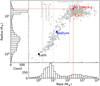 |
Fig. 1 Mass-radius distribution of the 5630 confirmed exoplanets to date (17 May 2024, Nasa Exoplanet Archive 2024). Not all the confirmed planets have a measured radius and/or mass, and thus the total count in the histograms is less than 5630. The scatter plot shows only the 596 planets for which the mass and radius are known within 15%. |
2 Observations
We observed four transits of HD 209458b in H-band with CRIRES+ (Follert et al. 2014) at the Very Large Telescope (VLT) as part of the ESO proposal 109.2376 (PI: Mollière). Obervations were taken in the nights of 29 June 2022, 6 July 2022, 12 October 2022, and 27 June 2023, called Night 1–4 in the following. We used a reference wavelength of 1567.099 nm and a slit width of 0.2″ for all nights, corresponding to spectral resolutions ≳100000. The observations were performed with the adaptive optics (AO) system MACAO (Arsenault et al. 2003), using the science target, HD 209458, as the AO star, allowing us to use the 0.2″ slit efficiently despite the larger seeing conditions. During nights 1–3, observations were taken in nodding mode with a 6″ nod throw. For Night 1 and 2 a detector integration time of DIT = 30 s was used, with six exposures per nodding position. For Night 3 this was changed to 3 exposures per nodding position. For Night 4 nodding was turned off, with a DIT of 20 s. Our observations were set up to avoid airmasses larger than 2, with total exposure times to cover the full transit, and to establish significant out-of-transit baseline observations. Typical execution times were of the order of 6 h. This results in 468, 600, 474, and 838 exposures taken for nights 1 to 4, respectively. The seeing was below 0.5″ during Night 1, between 0.5 and 1″ during Night 2, between 1 and 1.5″ during Night 3 and between 0.5 and 1.5″ during Night 4. The precipitable water vapors (PWV) were 1.5–1.6 mm, 1.5–2.5 mm, 1.5–1.7 mm, and 2.4–4.0 mm during nights 1 to 4, respectively.
The data were reduced using pycrires (Stolker & Landman 2023), which is a python wrapper for the official ESO CR2RES pipeline (Version 1.4.0)2. This pipeline includes the basic calibration steps, including dark and flat field correction, and optimally extracts the stellar spectrum. For the observations that were taken in nodding mode, we subtracted the background using an observation in the other nodding position. The Esorex pipeline by default combines all the exposures in the same nodding position, decreasing the temporal resolution. To avoid this, we run the pipeline on each nodding pair separately. We used each exposure only once, meaning that the first A exposure in a sequence was combined with the first B exposure, the second A exposure with the second B exposure, and so forth. In the spectral extraction we used an extraction height of 20 pixels, a swath width of 400 pixels, and an extraction oversampling of 10. Additionally, we turned off the subtract_no_light_rows, subtract_interorder_column and cosmic ray correction, as we found that these provided spurious values of certain spectral bins in the extracted spectrum. The wavelength solution was obtained using the Esorex pipeline and the calibration data from the Uranium-Neon lamp and the Fabry-Pérot etalon. However, we found slight inaccuracies in this wavelength solution by visually comparing it with a telluric model generated using SkyCalc. With CRIRES+, excellent seeing conditions (⪅1″) can lead the 0.2″ slit to receive a significantly non-uniform flux along its width, in an effect called ‘super-resolution’. In the case the position of the target on the slit changes with exposures, this can have a significant effect on the lines position (≈0.01 nm) and on the line spread function, while increasing the effective resolving power of the instrument. We therefore performed an additional correction on the wavelength solution using the correct_wavelengths method in pycrires, which is explained in Landman et al. (2024). An offset and linear correction to the wavelength solution from the Esorex pipeline were obtained by maximising the cross-correlation between the observed spectrum and a telluric model. We found that only small corrections to the original wavelength solution of <0.01 nm were required for this wavelength setting. The wavelength solution was subsequently verified through visual comparison with a telluric model.
3 Models
3.1 Self-consistent model
In order to have a robust first estimation of HD 209458 b’s atmospheric properties, we generate several self-consistent models using Exo-REM3. A summary of Exo-REM is provided in Blain et al. (2024), which is fully described by Baudino et al. (2015, 2017); Charnay et al. (2018); Blain et al. (2021).
Our HD 209458 b self-consistent models were parameterised following the same procedure described in Blain et al. (2021). The planet and star parameters used are displayed in Table 1.
HD 209458 b has a radius larger than expected by ‘baseline’ evolutionary models (e.g. Bodenheimer et al. 2001; Guillot & Showman 2002). As such, HD 209458 b falls into the category of ‘inflated’ planets. These larger radii has been attributed to hotter intrinsic temperatures than otherwise expected (Thorngren et al. 2020). Several mechanisms has been proposed to explain these hot interiors, including Ohmic dissipation (Batygin & Stevenson 2010; Laughlin et al. 2011), kinetic dissipation (Guillot & Showman 2002), or tidal dissipation (Bodenheimer et al. 2001). The latter however may be ruled out for HD 209458 b’s, due to the low eccentricity of the planet and apparent absence of another massive planet orbiting the star (Guillot & Showman 2002). In any case, because HD 209458 b is inflated, we use the model from Thorngren et al. (2020) to estimate its intrinsic temperature (Tp,int).
We include the radiative coupling of Fe, Mg2SiO4, and SiO2 clouds. We chose these condensates because their respective forming gases are the most abundant at the clouds pressures and temperatures of formation, according to our model. We use a cloud fraction of 0.8, which we estimate is reasonable, on average, in regard to 3-D simulations of the planet (e.g. Lines et al. 2018), and is also consistent with the value inferred by Xue et al. (2024). We use the wavelength- and particle radius-dependent optical constants (extinction coefficient, single-scattering albedo and asymmetry parameter) of Fe and Mg2SiO4 provided by Exo-REM. For SiO2, we use the refractive indices of Zeidler et al. (2013)4, and converted them to optical constants using the optpropgen code5. We use Exo-REM with the cloud model of Charnay et al. (2018) to self-consistently calculate the radius of the clouds particles, using a sticking efficiency of 1 and with a supersaturation parameter of 3 × 10⁻³.
We chose to use an atmospheric metallicity (Z) of 3 times the solar metallicity, which is the median value reported by Xue et al. (2024), and is consistent with the mass-metallicity trend observed in the Solar System and exoplanets in general (see e.g. Thorngren et al. 2016; Welbanks et al. 2019; Blain et al. 2021). We then compute three models with different C/O ratios, by varying the elemental abundance of C:
C/O = 0. 10: to match the median value reported by Xue et al. (2024),
C/O = 0.55: the solar C/O ratio (Lodders 2019),
C/O = 0.80: close to the C/O ratio reported by Giacobbe et al. (2021).
These C/O ratios above represent the bulk elemental abundances in the deep atmosphere, but due to cloud condensation, the effective C/O ratio in the upper atmosphere may be different. For example, our third model has an effective C/O ratio above the cloud condensation levels (≈103 Pa) of ≈1.
We were not able to obtain Exo-REM models at the same bulk C/O ratio as the best fit from Giacobbe et al. (2021) (≈0.95) due to the removal of H2O under these conditions. Since the Exo-REM chemical model base most of its calculations on the H2O abundance, its removal from the atmosphere makes it unstable. This low H2O abundance is due to a combination of factors. First, as the abundance of C increases, the atmospheric conditions of HD 209458 b favours the formation of CO at the detriment of H2O. At the same time, H2O is directly involved in the formation of Si-bearing condensates (Mg2SiO4, MgSiO3, SiO2). With a solar composition, silicon is ten times less abundant than oxygen (Lodders 2019). Hence, the condensations of Si-bearing species can efficiently remove H2O from the atmosphere if its abundance is sufficiently low. With most of the oxygen trapped in CO and Si-bearing condensates, the H2O volume mixing ratio can drop much below 10−10 above the SiO2 cloud formation level. On a side note, this might also prevent the complete removal of SiO from the upper atmosphere, making this species potentially detectable in that scenario.
The temperature profile and VMRs obtained are displayed in Figs. 2 and 3, respectively. The simulated spectra and absorber contributions for each model are displayed in Fig. 4.
3.2 Transmission spectrum model
3.2.1 Templates
We model the spectrum of HD 209458 b using the petitRADTRANS6 (pRT) package (Mollière et al. 2019). We follow the transmission spectrum construction method of Blain et al. (2024) to obtain our pressure grid, temperature profile (isothermal, with T = Teq), mass fractions (constant with pressure), and mean molar masses (their step 1). We also use their petitRADTRANS configuration (their step 3), and convolve the spectrum following their step 7 at the expected resolving power of CRIRES+ (ℛ = 92000). We also tested templates using ℛ = 100000, in order to take into account for the potential ‘super-resolution’ effect discussed in Sect. 2, but found no significant changes in our results. Their other steps, related to Doppler-shifting the lines, are skipped. The references for the line lists used are displayed in Table 2.
At first order, CCF analyses are sensitive to the line positions and shapes, but not to their absolute depth. Because of this, and because the template is not deformed in the same way as the observations by the preparing pipeline, this kind of analysis is reliable for species detection, but not for abundance estimation. Hence, the mass fractions of the species in the template model can be set to any value, as long as the lines of the tested species are prominent enough in the modelled spectrum.
We therefore use the same model basis in all of our templates: the mass fractions of all tested species are set to −3 log10(MMR), and H2 and He are added so that the sum of MMR is 1, with a He/H2 MMR ratio of 12/37, as in Blain et al. (2024). We also include the collision-induced absorptions of H2 and He, as well as their Rayleigh scattering effect. We do not include any cloud effect. Then, from this basis, we add the line-by-line (ℛ ≈ 106) opacities of only the tested species, which we down-sample by a factor of four to reduce memory usage. By cross-correlating these template spectra with the observations, we can thus test for the presence of individual species in the latter.
Parameters of HD 209458 b and its star.
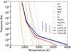 |
Fig. 2 Temperature profile and condensation curves obtained from our self-consistent model, for 3 times the solar metallicity. The blue, black, and red errorbars represent the pressure range concentrating 68% of the transmission contribution of our petitRADTRANS simulated data (see Sect. 3.2.2) over the data wavelength range, for a C/O ratio of 0.1, 0.55, and 0.8, respectively. |
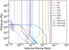 |
Fig. 3 Volume mixing ratios obtained from our self-consistent model, for 3 times the solar metallicity. Dotted: C/O = 0.1. Dashed: C/O = 0.55. Solid: C/O = 0.8. Only the most relevant absorbing species are represented. Na, K and PH3 are not represented due to their negligible contribution in our data wavelength coverage, while FeH, TiO and VO have VMRs lower than 10−10 at the pressure of maximum sensitivity. The blue, black, and red errorbars represent the pressure range concentrating 68% of the transmission contribution of our petitRADTRANS simulated data (see Sect. 3.2.2) over the data wavelength range, for a C/O ratio of 0.1, 0.55, and 0.8, respectively. |
 |
Fig. 4 HD 209458 b low-resolution (ℛ ≈ 500) transit depth and species contributions simulated with Exo-REM. The grey areas represent the wavelength range of the CRIRES+ orders. On top are indicated the orders index number. From top to bottom: models with a C/O ratio of 0.1, 0.55, and 0.8, respectively. Dotted: the combined contributions of the H2−H2 and H2−He collision-induced absorptions and the effect of Rayleigh scattering. Dashed: the total contribution of the SiO2, Mg2SiO3 and Fe clouds for a cloud coverage of 1.0. The contributions of CO2, FeH, K, Na, PH3, TiO and VO were negligible in this spectral region and thus are not represented. |
References of the line lists used for our high-resolution spectra.
3.2.2 Simulated data
We construct a total of nine different sets of simulated data, in a similar manner as the templates. We generate one set for each of our three Exo-REM models (see Sec. 3.1), in which we simulate the clouds by adding opaque layers down to the lowest pressure at which the sum of the cloud opacities reach 1 in the Exo-REM models (i.e. at 3.9, 4.4, and 4.1 log10(Pa), for a C/O ratio of 0.1, 0.55, and 0.8, respectively). We note that clouds form significantly deeper in our self-consistent Exo-REM models than inferred by Xue et al. (2024) with their free retrieval setup. Because of this, we generate three additional simulated data sets, where we fix the opaque layer lower pressure at 1.7 log10(Pa) (i.e. 50 Pa). For comparison, we also generate three models with no cloud coverage (opaque layer lower pressure fixed at 7 log10(Pa)). For the temperature profile, mass fractions7, and mean molar masses, we use the values obtained from our Exo-REM models, interpolated to the petitRADTRANS pressure grid. The species C2H2 is not implemented in Exo-REM, so we arbitrarily fix its abundance in all models to −8 log10(MMR).
We then modify the spectrum mostly following the simulated data construction procedure described in Blain et al. (2024), with Vrest = −5 km s−1. However, we skip their step 6 bis (the modelling of the telluric transmittances) and modify their step 9 (adding the instrumental deformations) as follows. We run the Polyfit (see Sec. 4.2) preparing pipeline on the real data, and retrieve the preparing matrix RF. This matrix is the element-wise multiplication of two second-order polynomial fits of the data. From Blain et al. (2024), if the time- and wavelength-dependent data F(t, λ) can be expressed as F = MΘ ∘ D + N, where the symbol ‘∘’ represents here the element-wise product (Million 2007), MΘ is an exact model of the planet’s spectrum with true parameters Θ, D is the deformation matrix, and N is the noise matrix, then the preparing matrix RF is proportional to 1 ⊘ D. Here the symbol ‘⊘’ represents the element-wise division (Wetzstein et al. 2012). We thus construct the simulated data Fsim as:
![Mathematical equation: $\[\mathbf{F}_{\mathrm{sim}}(t, \lambda)=\mathbf{M}_{\Theta}(t, \lambda) \oslash \mathbf{R}_{\mathbf{F}}(t, \lambda)+\mathbf{N}(t, \lambda),\]$](/articles/aa/full_html/2024/10/aa50767-24/aa50767-24-eq4.png) (1)
(1)
where here MΘ(t, λ) and N(t, λ) are obtained as in step 10 of Blain et al. (2024), using the same random seed (12345). The result is displayed in Fig. 5.
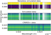 |
Fig. 5 Simulated data (Z = 3, C/O = 0.55, no cloud) and CRIRES+ data of night 3, for a section of order 14. Top row: simulated data with deformation matrix and noise matrix removed. The ‘well’ around orbital phase 0 is due to the modelled transitting effect. The spectral lines of the planet’s atmosphere can be seen within the ‘well’ as faint dark traces. Middle row: simulated data, including the approximated deformation matrix and the modelled noise matrix. Bottom row: real CRIRES+ data, for comparison. The white pixels are pixels masked during the Polyfit preparing pipeline and the trimming (see Sec. 4.2 of the observations). The spectra are represented in arbitrary units. |
4 Methods
4.1 Data selection
Order selection. The orders 0 to 2 (1.43–1.46 μm, see Fig. 4) of channel A are absent in channel B. For consistency, we remove these three orders from channel A. In addition, orders 3 to 5 (1.46–1.50 μm) are heavily contaminated by telluric lines, and we decided to discard these orders as well. As a result, we keep on both channel A and B orders 6 to 23, for a total of 18 orders.
Spectral pixel selection. Due to the bias subtraction as well as the loss of throughput at the edges of the orders, some spectral pixels on both sides of the orders present negative or near-zero values, that could affect our analysis. In order to avoid this, we discard the first ten and the last five spectral pixels of all orders, exposures, and nights. We thus keep 2033 spectral pixels on each order.
Bad pixels removal. After preparation (see Sec. 4.2), we note the presence of isolated ‘cold’ and ‘hot’ pixels, that might be caused by cosmic rays. We also note the presence of ‘dashed lines’, caused by spectral pixels presenting significantly more variations than their neighbours, at most but not all exposures, and inconsistent with the expected position of telluric or stellar lines (see Fig. 5, just after 1.622 μm). The origin of the latters might be instrumental, or created during the data reduction step. In order to avoid any bias caused by these pixels, we remove them by following the steps below:
We fit the observations with a second-order polynomial across wavelengths, for each exposure and each order, then divide the observations with the fit.
We mask the resulting spectra where their medians across exposures are greater than 1.2 and lower than 0.8, in each order and each wavelength.
We mask the 3σ outliers – determined from the mean and the standard deviation across all orders, exposures, and wavelengths – of the resulting masked spectra.
We fit the resulting masked spectra with a second-order polynomial across exposures, for each wavelength and each order, then divide them with the fit.
We mask the 3σ outliers – determined from the mean and the standard deviation across all orders, exposures, and wavelengths – of the resulting masked spectra.
In each order, we mask a spectral pixel in all the exposures if this spectral pixel was masked in at least 1 percent of the exposures with the previous treatment.
The resulting mask is then applied to the unaltered observations (i.e. the data before applying the steps above), before the preparing step (Sec. 4.2). The spectra resulting from the steps above are otherwise not used. Using this procedure, we increased the S/N metric of our H2O detection from 8.3 to 8.7σ (see Sec. 5.1). On average, considering only our 18 selected orders, and including the preparation step which masks the deepest telluric and stellar lines (see Sec. 4.2), we mask ≈20% of the pixels.
4.2 Preparing pipelines
As seen in Fig. 5, the observations (F) are dominated by telluric and stellar lines, as well as variation of observed flux level, pseudo-continuum, and blaze function (‘deformation matrix’). A crucial step of ground-based high-resolution data analysis is to remove as much as possible the deformation matrix in order to be left with only the planet’s signal. This is done with algorithms called ‘preparing pipelines’.
Polyfit. We use Polyfit (Blain et al. 2024) to generate mock observations, as described in Sect. 3.2.2. We follow Blain et al. (2024) and use second-order polynomials to fit both the instrumental deformations, and the telluric and stellar lines. We also mask the prepared data where the fit to the telluric and stellar lines is <0.8. The result of this preparing pipeline are the prepared data
![Mathematical equation: $\[P_{\mathbf{R}}(\mathbf{F}) \equiv \mathbf{F} \circ \mathbf{R}_{\mathbf{F}},\]$](/articles/aa/full_html/2024/10/aa50767-24/aa50767-24-eq5.png) (2)
(2)
where RF is the preparing matrix corresponding to F. The corresponding uncertainties are ![Mathematical equation: $\[\mathbf{U}_{\mathbf{R}} \equiv \mathbf{U} \circ\left|\mathbf{R}_{\mathbf{F}}\right| \circ \sqrt{n}\]$](/articles/aa/full_html/2024/10/aa50767-24/aa50767-24-eq6.png) , where U are the observations uncertainties, and n is the total variance correction factor of the two fits performed in Polyfit (see Blain et al. 2024).
, where U are the observations uncertainties, and n is the total variance correction factor of the two fits performed in Polyfit (see Blain et al. 2024).
SysRem. We use the SysRem (Tamuz et al. 2005) implementation described in Appendix B of Blain et al. (2024). We allow each passes to run 100 iterations until the convergence criterion (10−15) across all orders is reached. Thus, all orders are processed through the same number of iterations, and the same number of passes. The result of this preparing pipeline are the prepared data
![Mathematical equation: $\[P_{S, n}(\mathbf{F}) \equiv{ }^{(n)} \mathbf{F}_S={ }^{(n-1)} \mathbf{F}_S-\mathbf{a}_n \cdot \mathbf{c}_n,\]$](/articles/aa/full_html/2024/10/aa50767-24/aa50767-24-eq7.png) (3)
(3)
where n is the number of SysRem passes, ![Mathematical equation: $\[{ }^{(0)} \mathbf{F}_S \equiv \mathbf{F} \oslash \overline{\mathbf{X}}-\langle\mathbf{F} \oslash \overline{\mathbf{X}}\rangle_\lambda\]$](/articles/aa/full_html/2024/10/aa50767-24/aa50767-24-eq8.png) are the observations element-wise divided by their second-order polynomial fits along wavelength
are the observations element-wise divided by their second-order polynomial fits along wavelength ![Mathematical equation: $\[(\overline{\mathbf{X}})\]$](/articles/aa/full_html/2024/10/aa50767-24/aa50767-24-eq9.png) and mean-subtracted,
and mean-subtracted, ![Mathematical equation: $\[\langle\mathbf{F} \oslash \overline{\mathbf{X}}\rangle_\lambda\]$](/articles/aa/full_html/2024/10/aa50767-24/aa50767-24-eq10.png) is the mean of
is the mean of ![Mathematical equation: $\[\mathbf{F} \oslash \overline{\mathbf{X}}\]$](/articles/aa/full_html/2024/10/aa50767-24/aa50767-24-eq11.png) along wavelength, and an and cn are the vector along exposures and wavelengths, respectively, obtained by SysRem at pass n. The corresponding uncertainties are
along wavelength, and an and cn are the vector along exposures and wavelengths, respectively, obtained by SysRem at pass n. The corresponding uncertainties are ![Mathematical equation: $\[\mathbf{U}_S \equiv \mathbf{U} \oslash \overline{\mathbf{X}} \circ \sqrt{n_\lambda}\]$](/articles/aa/full_html/2024/10/aa50767-24/aa50767-24-eq12.png) , where nλ is the variance correction factor of the second-order polynomial fit along wavelength (see Blain et al. 2024).
, where nλ is the variance correction factor of the second-order polynomial fit along wavelength (see Blain et al. 2024).
4.3 Cross-correlation setup
In order to detect species in the atmosphere of HD 208458 b, we use the cross-correlation technique (e.g. Snellen et al. 2010; Brogi et al. 2018; Cabot et al. 2018; Hawker et al. 2018; Alonso-Floriano et al. 2019a; Sánchez-López et al. 2019, 2022), implemented in the redexo code8. After our data selection step described in Sec. 4.1, we prepare the data using SysRem as described in Sec. 4.2 to obtain the prepared data PS (F)(t, λ). We generate a template M as in Sect. 3.2.1. This template is then interpolated on Doppler-shifted wavelengths9, from a grid of rest velocities v between −200 and +200 km s−1 with a step of 1 km s−1 (for a total of 401 elements), to obtain the shifted templates Mshift(v, λ).
We then cross-correlate this grid of templates with the prepared data following
![Mathematical equation: $\[\operatorname{CCF}(t, v)=\sum_i \frac{P_{S, n}(\mathbf{F})\left(t, \lambda_i\right) \cdot\left(\mathbf{M}_{\text {shift }}\left(v, \lambda_i\right)-\left\langle\mathbf{M}_{\text {shift }}\right\rangle_\lambda(v)\right)}{\mathbf{U}_S^2\left(t, \lambda_i\right)},\]$](/articles/aa/full_html/2024/10/aa50767-24/aa50767-24-eq13.png) (4)
(4)
where i denotes the wavelength index, and ⟨Mshift⟩λ is the mean of Mshift along wavelength. The number of SysRem passes used n is discussed in Sec. 4.4. This process is repeated each night and channel10 for every order. Within a night/channel, we sum the CCFs of each order to obtain CCFo(t, v). An example of a CCFo map is displayed in Appendix A.
At this point we have one CCFo(t, v) per night and per channel. A good match between the template and the planet’s signal in the prepared data leaves a high correlation trace in CCFo(t, v), across exposures. However, this can be difficult to analyse, especially if the correlation with the signal is weak on individual exposure. We can use our knowledge on the expected planet’s radial velocity as seen by the observer (Vobs(t)) to ease the analysis. The velocity Vobs(t) can be written as (e.g. Blain et al. 2024)
![Mathematical equation: $\[V_{\text {obs }}(t)=v_0 \sin \left(i_p\right) ~\sin~ (2 \pi \phi(t))+V_{\text {sys }}+V_{\text {bary }}\]$](/articles/aa/full_html/2024/10/aa50767-24/aa50767-24-eq14.png) (5)
(5)
where v0 is the planet’s orbital velocity assuming a circular orbit, ip is the planet’s orbital inclination, ϕ is the orbital phase, Vsys is the systemic velocity, and Vbary is the barycentric velocity. We construct a grid of v0 from −50 to +250 km s−1 with a step of 1.3 km s−1 (for a total of 231 elements). This grid is translated into a grid of radial velocity semi-amplitudes (Kp = v0 sin(ip)) later, in post-processing. We then shift the rest frame of each CCFo at each exposure from v to v − Vobs(t), and sum the resulting map along exposures, ignoring out-of-transit exposures, to obtain a shifted cross-correlation map CCFshift(t, v) for each night and each channel.
To extract detection significance from CCFshift, two techniques are commonly used in the literature: the S/N metric (e.g. Brogi et al. 2018), and Welch’s t-test (Welch 1947). However, Cabot et al. (2018) reported that Welch’s t-test has a tendency to overestimate detection significance, due to oversampling11. Hence, we decided to use the more conservative S/N metric, while it also does not represent an accurate estimation of a species detection confidence (e.g. Cabot et al. 2018).
We first calculate the sum of CCFshift along exposures and nights/channels to obtain the co-added CCF map (CCFco). We then calculate the mean and the standard deviation of elements with a rest velocity outside the [−15, +15] km s−1 interval12, that is, the ‘out-of-trail’ elements of CCFco (CCFoot). The signal-to-noise ratio of the CCF is obtained via
![Mathematical equation: $\[\mathrm{S} / \mathrm{N}_{\mathrm{CCF}}\left(K_p, v\right)=\frac{\operatorname{CCF}_{\mathrm{co}}\left(K_p, v\right)-\left\langle\mathrm{CCF}_{\text {oot }}\left(K_p, v\right)\right\rangle_v}{\operatorname{std}_v\left(\mathrm{CCF}_{\text {oot }}\left(K_p, v\right)\right)},\]$](/articles/aa/full_html/2024/10/aa50767-24/aa50767-24-eq15.png) (6)
(6)
where stdv(x) represents the standard deviation of x along the rest velocities.
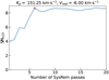 |
Fig. 6 S/NCCF (σ) combining the four nights from the H2O template at Kp = 151.25 km s−1 and Vrest = −6.00 km s−1, with respect to the number of SysRem passes. The red cross indicates the number of SysRem passes with which we chose to perform our analysis. |
4.4 Number of SysRem passes
As described in Sect. 4.2, the SysRem algorithm works by subtracting systematics from the data. Multiple passes can be applied, to remove ‘hidden’ linear trends. In principle, instrumental effects, telluric lines and stellar lines should create a limited number of linear trends. Applying too many passes may result in the removal of the planet’s signal (e.g. Blain et al. 2024). To estimate the optimal number of SysRem passes to apply, we follow Alonso-Floriano et al. (2019a) and calculate the S/N metric near the expected signal on our S/Nccf map for H2O, between 1 and 20 SysRem passes. The result is displayed in Fig. 6. The S/Nccf for H2O increases from approximately 4.0–8.7 when the number of SysRem passes is increased from 1 to 6. Further increases in SysRem passes does not significantly improves the S/Nccf. We decided to be conservative and chose to analyse the data prepared with six SysRem passes.
5 Results and discussion
We display the S/Nccf combining the four transits in Fig. 7. The value and location of the S/Nccf peak of each species is displayed in Table 3.
S/Nccf peak value and location for the tested species.
5.1 H2O and kinematics
Our H2O S/Nccf map is consistent with a planetary signal at ![Mathematical equation: $\[K_p=151.3_{-23.4}^{+31.1} \mathrm{~km} \mathrm{~s}^{-1}\]$](/articles/aa/full_html/2024/10/aa50767-24/aa50767-24-eq16.png) and
and ![Mathematical equation: $\[V_{\text {rest }}=-6_{-2}^{+1} \mathrm{~km} \mathrm{~s}^{-1}\]$](/articles/aa/full_html/2024/10/aa50767-24/aa50767-24-eq17.png) . The error bars of these values are obtained by taking the Kp and Vrest coordinates boundaries of the S/Nccf values greater or equal to the maximum S/Nccf (8.7), minus 1. The radial velocity semi-amplitude we obtain is consistent with the value expected from the literature (see Table 1): Kp = 149.4 ± 5.7 km s−1. Results using an alternative line list for water (HITEMP’s Rothman et al. 2010 instead of ExoMol’s Polyansky et al. 2018) are available in Appendix B.
. The error bars of these values are obtained by taking the Kp and Vrest coordinates boundaries of the S/Nccf values greater or equal to the maximum S/Nccf (8.7), minus 1. The radial velocity semi-amplitude we obtain is consistent with the value expected from the literature (see Table 1): Kp = 149.4 ± 5.7 km s−1. Results using an alternative line list for water (HITEMP’s Rothman et al. 2010 instead of ExoMol’s Polyansky et al. 2018) are available in Appendix B.
The blue-shifted rest velocity we obtain is consistent with the value reported by Gandhi et al. (2019) ![Mathematical equation: $\[\left(-3.0_{-1.6}^{+1.8} \mathrm{~km} \mathrm{~s}^{-1}\right)\]$](/articles/aa/full_html/2024/10/aa50767-24/aa50767-24-eq18.png) and Sánchez-López et al. (2019)
and Sánchez-López et al. (2019) ![Mathematical equation: $\[\left(-5.2_{-1.3}^{+1.6} \mathrm{~km} \mathrm{~s}^{-1}\right)\]$](/articles/aa/full_html/2024/10/aa50767-24/aa50767-24-eq19.png) , but not consistent with Snellen et al. (2010) (≈ −2 km s−1), and with Giacobbe et al. (2021), who did not report any significant Doppler-shift of the planet’s spectral features. Sánchez-López et al. (2019) discuss in details results from General Circulation Models (Rauscher & Menou 2012, 2013; Showman et al. 2012; Amundsen et al. 2016), concluding that their Vrest value is in good agreement with these models, except for the one presented in Rauscher & Menou (2013), which includes Ohmic dissipation that reduces wind speeds in the atmosphere. We note that a similar discrepancy in Vrest in the literature was highlighted for HD 189733 b by Blain et al. (2024), who suggested that inaccurate data timestamps could be a source of error when estimating this parameter.
, but not consistent with Snellen et al. (2010) (≈ −2 km s−1), and with Giacobbe et al. (2021), who did not report any significant Doppler-shift of the planet’s spectral features. Sánchez-López et al. (2019) discuss in details results from General Circulation Models (Rauscher & Menou 2012, 2013; Showman et al. 2012; Amundsen et al. 2016), concluding that their Vrest value is in good agreement with these models, except for the one presented in Rauscher & Menou (2013), which includes Ohmic dissipation that reduces wind speeds in the atmosphere. We note that a similar discrepancy in Vrest in the literature was highlighted for HD 189733 b by Blain et al. (2024), who suggested that inaccurate data timestamps could be a source of error when estimating this parameter.
5.2 Other species
We do not observe significant S/N metric peak for any of the other tested species. For C2H2, CH4, CO, CO2, HCN and NH3, the detected S/Nccf peak is ⪅4σ and situated at least more than 30 km s−1 from the expected planet signal in the Kp−Vrest space (see Table 3).
One species, H2S, show a ‘weak’ (⪅4σ) peak, but near the expected signal’s location. From Sect. 3.1, we expect H2S to be present in HD 209458 b’s atmosphere and to have a significant impact on its spectrum. While there is an informal convention in the literature to ignore ‘weak’ peaks, at face value, a spurious signal of 3.35σ or more still has a probability of only ≈4 × 10⁻⁴ to happen by chance.
To investigate if the peak we detect for H2S could arise from random fluctuations, we assume that our S/Nccf maps approximately follow a standard normal distribution, which can be expected from Eq. (6) if the observation noise is Gaussian. We then calculate the survivor function of the binomial distribution (the regularised incomplete beta function) for the number of S/NCCF values ≥3σ, Ip(k + 1, n − k), where p ≈ 1.35 × 10⁻³ is the probability to have S/NCCF values ≥3σ under our assumption, k is the number of S/NCCF values ≥3, and n = 92631 is the number of values in our S/NCCF maps. We finally translate the resulting probabilities into σ-significance. For H2S we have k = 115. For comparison, we obtain k = 2308 for H2O. The expected k in our case is ≈125.04, translating into a σ-significance of −0.85σ for H2S. In other words, the number of S/NCCF values ≥3σ for this species is slightly below what is expected for normally distributed samples of the size of our S/NCCF map. We conclude that the peak we observe for H2S is, similarly to the other species except H2O, not significant.
We note that the S/NCCF map of CH4 shows a significant anti-correlation peak of −5.3σ at Kp = 6 km s−1 and Vrest = 37 km s−1. This may be the result of remaining residuals. We performed an analysis using our CH4 template on the data prepared with 20 SysRem passes, but only managed to reduce the peak to −4.9σ, while the maximum remained both misplaced and <3.3σ. We conclude that, if this peak is caused by residuals, our SysRem implementation was not able to efficiently remove it. While it could be argued that this feature might hamper the detection of CH4 in our data, we note that, according to our results on simulated data, a simultaneous CH4 and H2O detection should be accompanied by at least a CO detection (see Table 4). We thus estimate that, even without this feature, it is unlikely that we would have been able to detect CH4.
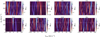 |
Fig. 7 CRIRES+ data: cross-correlation signal-to-noise ratio (S/NCCF) Kp−Vrest maps of all tested species. Negative values indicate an anti-correlation of the template with the data. The vertical and horizontal dashed lines show the expected Kp of the planet and the 0 km s−1 rest velocity, respectively. The red cross indicates the location of the maximum S/N. Rest velocities lower than −100 km s−1 and larger than +100 km s−1 are not shown for clarity. The maximum S/NCCF can be in this excluded region, hence the red cross is not on all figures. |
Simulated data: S/N metric peak value for the tested species in different atmospheric conditions.
5.3 Comparison with simulated data
5.3.1 Results
While a CCF analysis such as the one used in this work is inaccurate to estimate chemical abundances and other thermochemical properties (see Sect. 3.2.1), we can compare our results on the observations to those obtained with simulated datasets. This way, it is possible to check under which conditions detection or nondetection of a given species may be expected with our setup. We display the results for four of our nine simulated datasets in Fig. C.1, and for six of them in Table 4. We discuss the limits of this approach in Sect. 5.3.3. Hereafter we use the term ‘no detection’ when the maximum of a S/NCCF map is lower than 4σ.
The S/NCCF maps we obtain for our simulated data with C/O = 0.1 and Pc = 1.7 log10(Pa) are consistent with what we obtain with the observations: a significant H2O signal (11.9σ), and no detection otherwise. Results are similar when raising the C/O ratio to 0.55, but with a lower S/NCCF peak value (7.2σ) for H2O. There is no detection for any species with C/O = 0.8.
When using cloudless models (Pc = 7 log10(Pa)), we obtain, as expected, a stronger H2O S/Nccf peak with C/O = 0.1 and C/O = 0.55 (33.8σ and 32.2σ, respectively). By increasing the opaque cloud top pressure, we indeed lessen the cloud effect and increases the lines amplitude in the spectrum. However, H2O is still not detected with C/O = 0.8 (we obtain a peak of 4.4σ at Kp = 40.9 km s−1, but at the expected Kp the peak reaches only 2.8σ), mainly because of its low abundance, responsible for the low amplitude of its lines in the spectrum. Under these favourable cloud conditions, CH4 and HCN are detected only with C/O = 0.8 (12.2σ and 4.9σ, respectively), while NH3 is at the limit of detection (peak at 4.0σ). CO is detected only for C/O ≥ 0.55. H2S is detected at all the tested C/O ratios. On the other hand, C2H2 and CO2 are not detected in any simulated dataset. This result is expected for C2H2, given its artificially low abundance in our models, and for CO2, given its absence of significant spectral absorption in the CRIRES+ wavelength range observed in this study13.
Our results with the Exo-REM cloud models (Pc ≈ 4 log10(Pa)) show strong similarities with our results with the cloudless simulated data. The modelled opaque cloud layer is indeed located at too high pressures to significantly affect the spectrum. Similarly to the cloudless models, they do not reproduce the observations well. In addition, as mentioned in Sect. 3.2.2, this would also be inconsistent with the cloud pressure inferred by Xue et al. (2024). This suggests that the Exo-REM cloud model we used cannot accurately simulate cloud formation on HD 209458 b, or that different condensing species than the one implemented, or hazes, are involved.
These models also show that our non-detection of CO or CO2 in band H is not inconsistent with the detection of these species in other works (Snellen et al. 2010; Brogi & Line 2019; Gandhi et al. 2019; Xue et al. 2024). For CO, the reported detections were from band K (around 2.3 μm) observations, and the lowest reported abundance is from Brogi et al. (2017), with ![Mathematical equation: $\[-3.80_{-0.53}^{+0.51}\]$](/articles/aa/full_html/2024/10/aa50767-24/aa50767-24-eq20.png) log10(VMR), which is fully consistent with the log10(VMR) of our Exo-REM model with C/O = 0.1 and Z = 3 (≈ −3.6). For CO2, the detection (Xue et al. 2024) is inferred from its v3 band around 4.4 μm, and is consistent with a C/O ratio of 0.1.
log10(VMR), which is fully consistent with the log10(VMR) of our Exo-REM model with C/O = 0.1 and Z = 3 (≈ −3.6). For CO2, the detection (Xue et al. 2024) is inferred from its v3 band around 4.4 μm, and is consistent with a C/O ratio of 0.1.
It is worth noting that higher C/O ratios seem to favour H2S detection. While at constant metallicity, the abundance of H2S does not vary significantly with the C/O ratio (see Fig. 3, variations are caused by the slight changes in the temperature profile, affecting the chemical balance), the decrease in H2O abundance makes the H2S lines more prominent in the spectrum (see Fig. 4).
5.3.2 Possibility for a simultaneous detection of H2O and HCN in band H
Interestingly, even under the very favourable conditions of a cloudless atmosphere and a ‘perfect’ template, we are unable to detect both HCN and H2O with Z = 3 and a bulk C/O = 0.8 − effectively corresponding to C/O ≈ 1 above 103 Pa (see Sec. 3.1). HCN (and even more so NH3) are less than 1σ from the detection limit. Due to Exo-REM limitations, we did not investigate if the HCN (and NH3) S/NCCF would increase with a higher C/O ratio at this metallicity, but, in all cases, such an increase would make a H2O detection even less likely, due to its removal by Si-bearing condensates (as discussed in Sec. 3.1). We note that Giacobbe et al. (2021) reported that their chemical model does not take this effect into account. On the other hand, a lower Si/O ratio would allow for more H2O to remain above the cloud level, but to our knowledge there is no formation model considering this scenario in the literature. We also tested if increasing the metallicity to Z = 10 could allow for this simultaneous detection, but this was not the case (see Appendix D). In this scenario, only a 12% change in H2O abundance would have resulted in the complete removal (hence, undetectability) of this species. By staying in the upper atmosphere however, it seems to act as a screening for the HCN features, which as a consequence is no more detected.
Thus, it seems, according to our current knowledge and to our setup, that a simultaneous detection of HCN and H2O would indeed require a C/O ratio fine-tuned to an arguably extreme level, on top of requiring a cloudless (or an almost clear) atmosphere, which seems inconsistent with the observations (e.g, Sing et al. 2016; Pinhas et al. 2018; Giacobbe et al. 2021; Xue et al. 2024). However, an argument could be made that the terminator may have different C/O ratios: for example, one can imagine a hotter evening terminator where Si-bearing clouds did not condense, lowering in this region the effective (gas phase) C/O ratio, and increasing the H2O signal strength, while being at a high enough C/O in the gas phase at the colder morning terminator, due to nightside cloud condensation, such that carbon species such as CH4, HCN and C2H2 are at an increased abundance (see Sánchez-López et al. 2022, for more details on this scenario). We did not properly test this scenario in this work, but the 3-D model including cloud formation of HD 209458 b from Lines et al. (2018) do not predict an asymmetric cloud coverage along longitudes. According to a 2-D simulation, a relative chemical uniformity is expected across the planet (Tsai et al. 2024). A chemically asymmetric terminator scenario for HD 209458 b seems thus difficult to explain with current state-of-the-art models.
As previously mentioned, two previous works claimed a simultaneous detection of H2O and HCN in HD 209458b: Hawker et al. (2018) using VLT/CRIRES data and Giacobbe et al. (2021) using Telescopio Nazionale Galileo(TNG)/GIANO-B data, both at a high resolution. We note that Giacobbe et al. (2021) performed their CCF analysis only on the orders for which, for a given species, the detection of an injected signal was estimated sufficient. Several works (e.g. Debras et al. 2023; Blain et al. 2024), especially Cheverall et al. (2023), shown that this kind of procedure is likely to introduce biases in the analysis. Indeed, S/NCCF maps contains random fluctuations due to the cross-correlation of the template, mostly with noise. It is thus likely that this translates sometimes into positive correlations near the expected position in Kp−Vrest space. By selecting orders that favours the detection strength of an injected signal, there is a risk for a spurious signal to emerge from the combination of these favourable fluctuations. Hawker et al. (2018), instead, optimised the number of their Principal Component Analysis (PCA) preparing pipeline passes on each order for each species, as to maximise the detection of an injected signal. It is possible that this method also introduces biases by leaving in the prepared data systematics that would create spurious signals, although this specific case was not investigated in Cheverall et al. (2023). On the other hand, the wavelength range of Hawker et al. (2018) data (3.18–3.27 μm) is more favourable to HCN detection than ours (1.51–1.78 μm) and those of Giacobbe et al. (2021) (0.95–2.45 μm), due to the proximity of the strong HCN v1 fundamental band around 3.02 μm (e.g. Harris et al. 2006; Barber et al. 2014). In all cases, a re-analysis of these data without a data optimisation method would be useful to understand this discrepancy.
Comparison of this work with a selection of other HD 209458 b studies.
5.3.3 Summary
Our model with Z = 3, C/O = 0.1 and Pc = 1.7 log10(Pa) reproduces well our observations, although with a higher maximum S/NCCF. It appears clearly though that the strength of the H2O signal in the S/NCCF map can be decreased both by decreasing the pressure of the opaque cloud top layer, or by increasing the C/O ratio. We thus estimate that, according to our models, a higher C/O ratio and a higher opaque cloud top layer pressure are consistent with our observations, to a certain degree. With a C/O ratio of ≈0.8, we are not able to reproduce the observations, under any cloud condition. C/O ratios <0.1 and Pc < 1.7 log10(Pa) could also be possible. This is consistent with the results obtained by Xue et al. (2024), but not consistent with those inferred by Hawker et al. (2018) and Giacobbe et al. (2021). A comparison of our results with these studies is displayed in Table 5.
We note that a lower maximum S/NCCF than expected could also arise from imperfect line lists (see Appendix B), or residuals not captured by our simulated datasets. We note also that this conclusion comes from a limited parameter space exploration. Finally, these results are only valid for the unique noise realisation we tested. The S/N metric on those simulated data are expected to vary around their mean value with a standard deviation of 1, hence all species, especially those at the limit of detection, could be detected or undetected depending on whether or not the noise realisation is favourable.
6 Conclusion
We analysed CRIRES+ data of four HD 209458 b transits, covering wavelengths from 1.51 to 1.78 μm at a resolving power of ≈92000, and prepared with SysRem (Tamuz et al. 2005). Combining the four nights, our CCF analysis detects a H2O signal compatible with HD 209458 b at 8.68σ. We tested the data with C2H2, CH4, CO, CO2, H2S, HCN, and NH3, but did not detect any of these species.
In complement, we compared the above results with nine simulated datasets, using the temperature profiles and abundances from our self-consistent atmospheric model Exo-REM, spectra generated with petitRADTRANS, and deformations and uncertainties extracted from the observations. We found that our S/NCCF maps are consistent with a simulated dataset corresponding to Z = 3, C/O = 0.1 and Pc = 1.7 log10(Pa). However, the observations are also consistent, at this metallicity, with a combination of higher C/O ratios and higher opaque cloud top pressures, but not with cloudless atmospheres with a C/O ratio ≥ 0.55, and not under any cloud condition with a C/O ratio of 0.8. Indeed, increasing the C/O ratio decreases the strength of the H2O signal, due to chemical process favouring the formation of CO when more carbon is available, and due to the removal of H2O because of the condensation of Si-bearing species. In contrast, increasing the opaque cloud top pressure increases the signal of all species, due to the removal of the cloud’s spectral dampening effect.
With these models, we also show that a simultaneous detection of HCN and H2O in HD 209458 b’s atmosphere with CRIRES+ in band H, even when using a very specific C/O value, seems unlikely. This would require a different HCN chemical model – or a different cloud formation model – than the one we used, or strong regional chemical discrepancies in HD 209458 b, which does not seem to be expected (Lines et al. 2018; Tsai et al. 2024). Our non-detection of any species except H2O is not consistent with the detection of C2H2, CH4, HCN and NH3 by Giacobbe et al. (2021) from GIANO-B data. Instead, our results are consistent with those obtained by Xue et al. (2024), from JWST observations.
Acknowledgements
The authors thank A. Sánchez-López for his precious help with the observation setup. This research has made use of the NASA Exoplanet Archive, which is operated by the California Institute of Technology, under contract with the National Aeronautics and Space Administration under the Exoplanet Exploration Program. This research has made use of the Exoplanet Follow-up Observation Program (ExoFOP; DOI: 10.26134/ExoFOP5) website, which is operated by the California Institute of Technology, under contract with the National Aeronautics and Space Administration under the Exoplanet Exploration Program.
Appendix A Example of a CCFo map
In Fig. A.1 we represent the CCFo map obtained on the observations for night 3, channel B, using the H2O template. For comparison, we display the same map obtained with simulated data in Fig. A.2, assuming a cloudless atmosphere.
 |
Fig. A.1 CRIRES+ data: CCFo map for night 3, channel B, using the H2O template. The horizontal white lines represent the orbital phases of the HD 209458 b’s expected transit ingress (bottom) and egress (top). The slanted line represent HD 209458 b’s expected radial velocities, corrected from the barycentric velocities, with Vrest = 0 km s−1. Rest velocities lower than −25 km·s−1 and larger than +35 km·s−1 are not shown for clarity. |
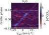 |
Fig. A.2 Simulated data: CCFo map for night 3, channel B, using the H2O template. The model has Z = 3, C/O = 0.1 and no cloud. The horizontal white lines represent the orbital phases of the HD 209458 b’s expected transit ingress (bottom) and egress (top). The slanted line represent HD 209458 b’s expected radial velocities, corrected from the barycentric velocities, with Vrest = 0 km·s−1. Rest velocities lower than −25 km·s−1 and larger than +35 km·s−1 are not shown for clarity. |
Appendix B Results using the H2O HITEMP line list
In addition to our main analysis using the POKAZATEL (Polyansky et al. 2018, see Table 2) H2O line list, we also performed an analysis using the H2O line list from the HITEMP database (Rothman et al. 2010). The S/Nccf maps for the observations and a selection of simulated data are displayed in Fig. B.1 and Fig. B.2, respectively.
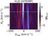 |
Fig. B.1 CRIRES+ data: cross-correlation signal-to-noise ratio (S/Nccf) Kp−Vrest maps using a H2O template with the HITEMP line list. Negative values indicate an anti-correlation of the template with the data. The vertical and horizontal dashed lines show the expected Kp of the planet and the 0 km·s−1 rest velocity, respectively. The red cross indicates the emplacement of the maximum S/N. Rest velocities lower than −100 km·s−1 and larger than +100 km·s−1 are not shown for clarity. |
 |
Fig. B.2 Simulated data: cross-correlation signal-to-noise ratio (S/NCCF) Kp−Vrest maps using a H2O template with the HITEMP line list for a selection of simulated datasets constructed with the POKAZATEL H2O line list. The leftmost column displays the results obtained with a C/O ratio of 0.1, and an opaque cloud top pressure of 1.7 log10(Pa). Going to the right, the columns display the results from cloudless (Pc = 7 log10(Pa)) simulated datasets, with C/O ratio of 0.1, 0.55, and 0.8, respectively. Negative values indicate an anti-correlation of the template with the data. The vertical and horizontal dashed lines show the expected Kp of the planet and the 0 km·s−1 rest velocity, respectively. The red cross indicates the location of the maximum S/N. Rest velocities lower than −100 km·s−1 and larger than +100 km·s−1 are not shown for clarity. |
We observe a S/Nccf peak of 7.3σ at ![Mathematical equation: $\[K_p=145.0_{-1}^{+103} \mathrm{~km} {\cdot} \mathrm{s}^{-1}\]$](/articles/aa/full_html/2024/10/aa50767-24/aa50767-24-eq24.png) and
and ![Mathematical equation: $\[V_{\text {rest }}=-6_{-1}^{+5} \mathrm{~km} {\cdot} \mathrm{s}^{-1}\]$](/articles/aa/full_html/2024/10/aa50767-24/aa50767-24-eq25.png) . The constraints and peak value are thus slightly less significant than using the POKAZATEL line list, but the results are otherwise similar.
. The constraints and peak value are thus slightly less significant than using the POKAZATEL line list, but the results are otherwise similar.
We performed the same analysis on our simulated data, using a H2O HITEMP template on a spectra generated with the POKAZATEL line list. This results as expected in a significantly decreased S/Nccf peak for the cloudless case (≈ −6σ compared to the POKAZTEL-on-POKAZATEL results). On the cloudy case, the effect is less impactful with a loss of only ≈ −2σ.
Appendix C Results on simulated data with Z = 3
In Fig. C.1 we display the S/Nccf maps of four of our nine simulated datasets.
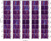 |
Fig. C.1 Simulated data: cross-correlation signal-to-noise ratio (S/NCCF) Kp−Vrest maps of all tested species. Each row displays the map corresponding to a different species. The leftmost column displays the results obtained with a C/O ratio of 0.1, and an opaque cloud top pressure of 1.7 log10(Pa). Going to the right, the columns display the results from cloudless (Pc = 7 log10(Pa)) simulated datasets, with C/O ratio of 0.1, 0.55, and 0.8, respectively. Negative values indicate an anti-correlation of the template with the data. The vertical and horizontal dashed lines show the expected Kp of the planet and the 0 km·s−1 rest velocity, respectively. The red cross indicates the location of the maximum S/N. Rest velocities lower than −100 km·s−1 and larger than +100 km·s−1 are not shown for clarity. The maximum S/NCCF can be in this excluded region, hence the red cross is not on all figures. All simulated data use the same noise seed, hence random features are the same on different models. |
Appendix D Results on simulated data with C/O = 0.8 and Z = 10
In complement to our simulated data at Z = 3, we also tested if a cloudless model at Z = 10 and C/O = 0.8 would allow for a simultaneous detection of H2O and HCN. The results are displayed in Fig. D.1.
The S/Nccf in this scenario are similar to those obtained with at C/O = 0.8 and Z = 3. HCN is this time undetected (the peak is misplaced and at 3.7σ), but H2O is detected with a peak at 13.5σ. NH3 is also undetected, with a misplaced peak at 3.8σ.
By increasing the metallicity, we increase the amount of absorbing gases in the atmosphere, hence the temperature, which rises at all layers by ≈ 50 K. This slightly shifts the H2O–SiO chemical balance so that H2O ends up slightly more abundant (≈ 12%) than SiO at the SiO2 condensation layer, preventing the complete removal of H2O from the atmosphere. The overall higher temperatures also favour the formation of CO and CO2 at the detriment of CH4. With less of the latter available, and despite a more metallic atmosphere and a more favourable kinematic balance, the HCN abundance only increases by ≈ 15% compared to the Z = 3 case, below the CH4/HCN quench pressure at ≈ 4.8 log10(Pa).
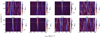 |
Fig. D.1 Simulated data: cross-correlation signal-to-noise ratio (S/NCCF) Kp−Vrest maps of all tested species, using a simulated dataset with C/O = 0.8 and Z = 10, and no cloud (Pc = 7 log10(Pa)). Negative values indicate an anti-correlation of the template with the data. The vertical and horizontal dashed lines show the expected Kp of the planet and the 0 km·s−1 rest velocity, respectively. The red cross indicates the location of the maximum S/N. Rest velocities lower than −100 km·s−1 and larger than +100 km·s−1 are not shown for clarity. The maximum S/NCCF can be in this excluded region, hence the red cross is not on all figures. |
References
- Alonso-Floriano, F., Sánchez-López, A., Snellen, I., et al. 2019a, A&A, 621, A74 [NASA ADS] [CrossRef] [EDP Sciences] [Google Scholar]
- Alonso-Floriano, F. J., Snellen, I. A. G., Czesla, S., et al. 2019b, A&A, 629, A110 [NASA ADS] [CrossRef] [EDP Sciences] [Google Scholar]
- Amundsen, D. S., Mayne, Nathan J., Baraffe, Isabelle, et al. 2016, A&A, 595, A36 [NASA ADS] [CrossRef] [EDP Sciences] [Google Scholar]
- Arsenault, R., Alonso, J., Bonnet, H., et al. 2003, SPIE, 4839, 174 [NASA ADS] [Google Scholar]
- Barber, R. J., Strange, J. K., Hill, C., et al. 2014, MNRAS, 437, 1828 [CrossRef] [Google Scholar]
- Batygin, K., & Stevenson, D. J. 2010, ApJ, 714, L238 [NASA ADS] [CrossRef] [Google Scholar]
- Baudino, J. L., Bézard, B., Boccaletti, A., et al. 2015, A&A, 582, A83 [NASA ADS] [CrossRef] [EDP Sciences] [Google Scholar]
- Baudino, J. L., Mollière, P., Venot, O., et al. 2017, ApJ, 850, 150 [NASA ADS] [CrossRef] [Google Scholar]
- Beaulieu, J. P., Kipping, D. M., Batista, V., et al. 2010, MNRAS, 409, 963 [Google Scholar]
- Blain, D., Charnay, B., & Bézard, B. 2021, A&A, 646, A15 [EDP Sciences] [Google Scholar]
- Blain, D., Sánchez-López, A., & Mollière, P. 2024, AJ 167, 179 [NASA ADS] [CrossRef] [Google Scholar]
- Bodenheimer, P., Lin, D. N. C., & Mardling, R. A. 2001, ApJ, 548, 466 [NASA ADS] [CrossRef] [Google Scholar]
- Bonomo, A. S., Desidera, S., Benatti, S., et al. 2017, A&A, 602, A107 [NASA ADS] [CrossRef] [EDP Sciences] [Google Scholar]
- Booth, R. A., Clarke, C. J., Madhusudhan, N., & Ilee, J. D. 2017, MNRAS, 469, 3994 [Google Scholar]
- Brogi, M., & Line, M. R. 2019, ApJ, 157, 114 [Google Scholar]
- Brogi, M., Line, M., Bean, J., Désert, J.-M., & Schwarz, H. 2017, ApJ, 839, L2 [NASA ADS] [CrossRef] [Google Scholar]
- Brogi, M., Giacobbe, P., Guilluy, G., et al. 2018, A&A, 615, A16 [NASA ADS] [CrossRef] [EDP Sciences] [Google Scholar]
- Cabot, S. H. C., Madhusudhan, N., Hawker, G. A., & Gandhi, S. 2018, MNRAS, 482, 4422 [Google Scholar]
- Cavalié, T., Lunine, J., Mousis, O., & Hueso, R. 2024, Space Sci. Rev., 220, 8 [CrossRef] [Google Scholar]
- Charnay, B., Bézard, B., Baudino, J. L., et al. 2018, ApJ, 854, 172 [Google Scholar]
- Cheverall, C. J., Madhusudhan, N., & Holmberg, M. 2023, MNRAS, 522, 661 [NASA ADS] [CrossRef] [Google Scholar]
- Coles, P. A., Yurchenko, S. N., & Tennyson, J. 2019, MNRAS, 490, 4638 [CrossRef] [Google Scholar]
- Cubillos, P. E., Fossati, L., Koskinen, T., et al. 2020, AJ, 159, 111 [Google Scholar]
- Database of Optical Constants for Cosmic Dust. 2024, Optical Constants of Crystalline Silicates, https://www.astro.uni-jena.de/Laboratory/OCDB/ [Online; accessed 08-March-2024] [Google Scholar]
- Debras, F., Klein, B., Donati, J.-F., et al. 2023, MNRAS, 527, 566 [NASA ADS] [CrossRef] [Google Scholar]
- del Burgo, C., & Allende Prieto, C. 2016, MNRAS, 463, 1400 [CrossRef] [Google Scholar]
- Deming, D., Wilkins, A., McCullough, P., et al. 2013, ApJ, 774, 95 [Google Scholar]
- ExoFOP website 2024, ExoFOP website, https://exofop.ipac.caltech.edu/tess/target.php?id=420814525 [Online; accessed 05-March-2024] [Google Scholar]
- Follert, R., Dorn, R. J., Oliva, E., et al. 2014, SPIE Conf. Ser., 9147, 914719 [Google Scholar]
- Gandhi, S., Madhusudhan, N., Hawker, G., & Piette, A. 2019, AJ, 158, 228 [NASA ADS] [CrossRef] [Google Scholar]
- Gautier, D., & Hersant, F. 2005, Space Sci. Rev., 116, 25 [NASA ADS] [CrossRef] [Google Scholar]
- Giacobbe, P., Brogi, M., Gandhi, S., et al. 2021, Nature, 592, 205 [NASA ADS] [CrossRef] [Google Scholar]
- Guillot, T., & Showman, A. P. 2002, A&A, 385, 156 [NASA ADS] [CrossRef] [EDP Sciences] [Google Scholar]
- Hargreaves, R. J., Gordon, I. E., Rey, M., et al. 2020, ApJS, 247, 55 [NASA ADS] [CrossRef] [Google Scholar]
- Harris, G. J., Tennyson, J., Kaminsky, B. M., Pavlenko, Y. V., & Jones, H. R. A. 2006, MNRAS, 367, 400 [Google Scholar]
- Hawker, G. A., Madhusudhan, N., Cabot, S. H. C., & Gandhi, S. 2018, ApJ, 863, L11 [NASA ADS] [CrossRef] [Google Scholar]
- Kempton, E. M.-R., Bean, J. L., Louie, D. R., et al. 2018, PASP, 130, 114401 [CrossRef] [Google Scholar]
- Landman, R., Stolker, T., Snellen, I. A. G., et al. 2024, A&A, 682, A48 [NASA ADS] [CrossRef] [EDP Sciences] [Google Scholar]
- Laughlin, G., Crismani, M., & Adams, F. C. 2011, ApJ, 729, L7 [NASA ADS] [CrossRef] [Google Scholar]
- Lines, S., Mayne, N. J., Boutle, I. A., et al. 2018, A&A, 615, A97 [NASA ADS] [CrossRef] [EDP Sciences] [Google Scholar]
- Lira-Barria, A., Rojo, P. M., & Mendez, R. A. 2022, A&A, 657, A36 [NASA ADS] [CrossRef] [EDP Sciences] [Google Scholar]
- Lodders, K. 2004, ApJ, 611, 587 [NASA ADS] [CrossRef] [Google Scholar]
- Lodders, K. 2019, Solar Elemental Abundances (Oxford: Oxford University Press) [Google Scholar]
- MacDonald, R. J., & Madhusudhan, N. 2017, MNRAS, 469, 1979 [Google Scholar]
- Madhusudhan, N., Amin, M. A., & Kennedy, G. M. 2014a, ApJ, 794, L12 [Google Scholar]
- Madhusudhan, N., Crouzet, N., McCullough, P. R., Deming, D., & Hedges, C. 2014b, ApJ, 791, L9 [Google Scholar]
- Million, E. 2007, in The Hadamard Product, 1 Introduction and Basic Results (Berlin: Springer) [Google Scholar]
- Mollière, P., van Boekel, R., Dullemond, C., Henning, T., & Mordasini, C. 2015, ApJ, 813, 47 [Google Scholar]
- Mollière, P., Wardenier, J. P., van Boekel, R., et al. 2019, A&A, 627, A67 [Google Scholar]
- Mollière, P., Molyarova, T., Bitsch, B., et al. 2022, ApJ, 934, 74 [CrossRef] [Google Scholar]
- Monga, N., & Desch, S. 2014, ApJ, 798, 9 [NASA ADS] [CrossRef] [Google Scholar]
- Mordasini, C., van Boekel, R., Mollière, P., Henning, T., & Benneke, B. 2016, ApJ, 832, 41 [Google Scholar]
- Naef, D., Mayor, M., Beuzit, J. L., et al. 2004, A&A, 414, 351 [NASA ADS] [CrossRef] [EDP Sciences] [Google Scholar]
- Nasa Exoplanet Archive 2024, Planetary Systems Table, https://exoplanetarchive.ipac.caltech.edu/cgi-bin/TblView/nph-tblView?app=ExoTbls&config=PS [Online; accessed 05-March-2024] [Google Scholar]
- Öberg, K. I., Murray-Clay, R., & Bergin, E. A. 2011, ApJ, 743, L16 [Google Scholar]
- Pekmezci, G. S., Johnson, T. V., Lunine, J. I., & Mousis, O. 2019, ApJ, 887, 3 [NASA ADS] [CrossRef] [Google Scholar]
- Pinhas, A., Madhusudhan, N., Gandhi, S., & MacDonald, R. 2018, MNRAS, 482, 1485 [Google Scholar]
- Polyansky, O. L., Kyuberis, A. A., Zobov, N. F., et al. 2018, MNRAS, 480, 2597 [NASA ADS] [CrossRef] [Google Scholar]
- Rauscher, E., & Menou, K. 2012, ApJ, 750, 96 [NASA ADS] [CrossRef] [Google Scholar]
- Rauscher, E., & Menou, K. 2013, ApJ, 764, 103 [NASA ADS] [CrossRef] [Google Scholar]
- Rothman, L. S., Gordon, I. E., Barber, R. J., et al. 2010, J. Quant. Spectr. Rad. Transf., 111, 2139 [Google Scholar]
- Rothman, L. S., Gordon, I. E., Babikov, Y., et al. 2013, J. Quant. Spectr. Rad. Transf., 130, 4 [Google Scholar]
- Schwarz, H., Brogi, M., de Kok, R., Birkby, J., & Snellen, I.. 2015, A&A, 576, A111 [NASA ADS] [CrossRef] [EDP Sciences] [Google Scholar]
- Showman, A. P., Fortney, J. J., Lewis, N. K., & Shabram, M. 2012, ApJ, 762, 24 [Google Scholar]
- Sing, D. K., Fortney, J. J., Nikolov, N., et al. 2016, Nature, 529, 59 [Google Scholar]
- Snellen, I. A., De Kok, R. J., De Mooij, E. J., & Albrecht, S. 2010, Nature, 465, 1049 [NASA ADS] [CrossRef] [Google Scholar]
- Stassun, K. G., Collins, K. A., & Gaudi, B. S. 2017, AJ, 153, 136 [Google Scholar]
- Stolker, T., & Landman, R. 2023, Astrophysics Source Code Library [record ascl:2307.040] [Google Scholar]
- Sánchez-López, A., Alonso-Floriano, F. J., López-Puertas, M., et al. 2019, A&A, 630, A53 [NASA ADS] [CrossRef] [EDP Sciences] [Google Scholar]
- Sánchez-López, A., Landman, R., Mollière, P., et al. 2022, A&A, 661, A78 [NASA ADS] [CrossRef] [EDP Sciences] [Google Scholar]
- Tamuz, O., Mazeh, T., & Zucker, S. 2005, MNRAS, 356, 1466 [Google Scholar]
- Thorngren, D. P., Fortney, J. J., Murray-Clay, R. A., & Lopez, E. D. 2016, ApJ, 831, 64 [NASA ADS] [CrossRef] [Google Scholar]
- Thorngren, D., Gao, P., & Fortney, J. J. 2020, ApJ, 889, L39 [NASA ADS] [CrossRef] [Google Scholar]
- Tsai, S.-M., Parmentier, V., Mendonça, J. M., et al. 2024, ApJ, 963, 41 [NASA ADS] [CrossRef] [Google Scholar]
- Tsiaras, A., Waldmann, I. P., Zingales, T., et al. 2018, AJ, 155, 156 [NASA ADS] [CrossRef] [Google Scholar]
- Welbanks, L., Madhusudhan, N., Allard, N. F., et al. 2019, ApJ, 887, L20 [NASA ADS] [CrossRef] [Google Scholar]
- Welch, B. L. 1947, Biometrika, 34, 28 [Google Scholar]
- Wetzstein, G., Lanman, D., Hirsch, M., & Raskar, R. 2012, ACM Trans. Graph., 31, 1 [CrossRef] [Google Scholar]
- Xue, Q., Bean, J. L., Zhang, M., et al. 2024, ApJ, 963, L5 [NASA ADS] [CrossRef] [Google Scholar]
- Yurchenko, S. N., Mellor, T. M., Freedman, R. S., & Tennyson, J. 2020, MNRAS, 496, 5282 [NASA ADS] [CrossRef] [Google Scholar]
- Zeidler, S., Posch, Th., & Mutschke, H. 2013, A&A, 553, A81 [NASA ADS] [CrossRef] [EDP Sciences] [Google Scholar]
The data taken by Xue et al. (2024) contain the strong CO2 v3 band at ≈4 μm (see e.g. Yurchenko et al. 2020). However, CO2 does not have significant spectral features in band H, hence it cannot be detected from our dataset (see Sects. 3.1 and 5.3.1).
Acquired from the Database of Optical Constants for Cosmic Dust (2024), SiO2 at 928 K, E || c.
Code developed by F. Montmessin and J.-B. Madeleine at LATMOS/LMD, and available on the Exo-REM reporitory.
For the conversion, ![Mathematical equation: $\[X_i=\frac{M_i}{M} V_i\]$](/articles/aa/full_html/2024/10/aa50767-24/aa50767-24-eq26.png) , where Xi, Mi, and Vi are the mass fraction, molar mass and volume mixing ratio of species i, respectively, and M is the mean molar mass of the atmosphere.
, where Xi, Mi, and Vi are the mass fraction, molar mass and volume mixing ratio of species i, respectively, and M is the mean molar mass of the atmosphere.
Using the non-relativistic approximation: λshift = λ(1 − v/c), where c is the speed of light in vacuum.
There are four nights, three nights have two channels, one night have one channel. Hence, there is a total of seven night/channel entities.
Welch’s t-test makes the assumption that the two samples are random drawn from normal distributions. In the context of a CCF analysis, this is approximately the case for the out-of-trail sample, but not for the in-trail sample, due to the high correlation of its values. See also Cheverall et al. (2023).
Excluding 15 elements centred on 0 km s−1, resulting in a sample of 370 (= 401–31) elements. The choice of this interval is arbitrary.
We note that assuming a bulk C/O ratio >1, C2H2 and HCN are expected to be the major C-bearing species behind CO, and above CH4, see e.g. Mollière et al. (2015). These species may thus be detectable in band H at these higher C/O ratios.
All Tables
Simulated data: S/N metric peak value for the tested species in different atmospheric conditions.
All Figures
|
Fig. 1 Mass-radius distribution of the 5630 confirmed exoplanets to date (17 May 2024, Nasa Exoplanet Archive 2024). Not all the confirmed planets have a measured radius and/or mass, and thus the total count in the histograms is less than 5630. The scatter plot shows only the 596 planets for which the mass and radius are known within 15%. |
| In the text | |
|
Fig. 2 Temperature profile and condensation curves obtained from our self-consistent model, for 3 times the solar metallicity. The blue, black, and red errorbars represent the pressure range concentrating 68% of the transmission contribution of our petitRADTRANS simulated data (see Sect. 3.2.2) over the data wavelength range, for a C/O ratio of 0.1, 0.55, and 0.8, respectively. |
| In the text | |
|
Fig. 3 Volume mixing ratios obtained from our self-consistent model, for 3 times the solar metallicity. Dotted: C/O = 0.1. Dashed: C/O = 0.55. Solid: C/O = 0.8. Only the most relevant absorbing species are represented. Na, K and PH3 are not represented due to their negligible contribution in our data wavelength coverage, while FeH, TiO and VO have VMRs lower than 10−10 at the pressure of maximum sensitivity. The blue, black, and red errorbars represent the pressure range concentrating 68% of the transmission contribution of our petitRADTRANS simulated data (see Sect. 3.2.2) over the data wavelength range, for a C/O ratio of 0.1, 0.55, and 0.8, respectively. |
| In the text | |
|
Fig. 4 HD 209458 b low-resolution (ℛ ≈ 500) transit depth and species contributions simulated with Exo-REM. The grey areas represent the wavelength range of the CRIRES+ orders. On top are indicated the orders index number. From top to bottom: models with a C/O ratio of 0.1, 0.55, and 0.8, respectively. Dotted: the combined contributions of the H2−H2 and H2−He collision-induced absorptions and the effect of Rayleigh scattering. Dashed: the total contribution of the SiO2, Mg2SiO3 and Fe clouds for a cloud coverage of 1.0. The contributions of CO2, FeH, K, Na, PH3, TiO and VO were negligible in this spectral region and thus are not represented. |
| In the text | |
|
Fig. 5 Simulated data (Z = 3, C/O = 0.55, no cloud) and CRIRES+ data of night 3, for a section of order 14. Top row: simulated data with deformation matrix and noise matrix removed. The ‘well’ around orbital phase 0 is due to the modelled transitting effect. The spectral lines of the planet’s atmosphere can be seen within the ‘well’ as faint dark traces. Middle row: simulated data, including the approximated deformation matrix and the modelled noise matrix. Bottom row: real CRIRES+ data, for comparison. The white pixels are pixels masked during the Polyfit preparing pipeline and the trimming (see Sec. 4.2 of the observations). The spectra are represented in arbitrary units. |
| In the text | |
|
Fig. 6 S/NCCF (σ) combining the four nights from the H2O template at Kp = 151.25 km s−1 and Vrest = −6.00 km s−1, with respect to the number of SysRem passes. The red cross indicates the number of SysRem passes with which we chose to perform our analysis. |
| In the text | |
|
Fig. 7 CRIRES+ data: cross-correlation signal-to-noise ratio (S/NCCF) Kp−Vrest maps of all tested species. Negative values indicate an anti-correlation of the template with the data. The vertical and horizontal dashed lines show the expected Kp of the planet and the 0 km s−1 rest velocity, respectively. The red cross indicates the location of the maximum S/N. Rest velocities lower than −100 km s−1 and larger than +100 km s−1 are not shown for clarity. The maximum S/NCCF can be in this excluded region, hence the red cross is not on all figures. |
| In the text | |
|
Fig. A.1 CRIRES+ data: CCFo map for night 3, channel B, using the H2O template. The horizontal white lines represent the orbital phases of the HD 209458 b’s expected transit ingress (bottom) and egress (top). The slanted line represent HD 209458 b’s expected radial velocities, corrected from the barycentric velocities, with Vrest = 0 km s−1. Rest velocities lower than −25 km·s−1 and larger than +35 km·s−1 are not shown for clarity. |
| In the text | |
|
Fig. A.2 Simulated data: CCFo map for night 3, channel B, using the H2O template. The model has Z = 3, C/O = 0.1 and no cloud. The horizontal white lines represent the orbital phases of the HD 209458 b’s expected transit ingress (bottom) and egress (top). The slanted line represent HD 209458 b’s expected radial velocities, corrected from the barycentric velocities, with Vrest = 0 km·s−1. Rest velocities lower than −25 km·s−1 and larger than +35 km·s−1 are not shown for clarity. |
| In the text | |
|
Fig. B.1 CRIRES+ data: cross-correlation signal-to-noise ratio (S/Nccf) Kp−Vrest maps using a H2O template with the HITEMP line list. Negative values indicate an anti-correlation of the template with the data. The vertical and horizontal dashed lines show the expected Kp of the planet and the 0 km·s−1 rest velocity, respectively. The red cross indicates the emplacement of the maximum S/N. Rest velocities lower than −100 km·s−1 and larger than +100 km·s−1 are not shown for clarity. |
| In the text | |
|
Fig. B.2 Simulated data: cross-correlation signal-to-noise ratio (S/NCCF) Kp−Vrest maps using a H2O template with the HITEMP line list for a selection of simulated datasets constructed with the POKAZATEL H2O line list. The leftmost column displays the results obtained with a C/O ratio of 0.1, and an opaque cloud top pressure of 1.7 log10(Pa). Going to the right, the columns display the results from cloudless (Pc = 7 log10(Pa)) simulated datasets, with C/O ratio of 0.1, 0.55, and 0.8, respectively. Negative values indicate an anti-correlation of the template with the data. The vertical and horizontal dashed lines show the expected Kp of the planet and the 0 km·s−1 rest velocity, respectively. The red cross indicates the location of the maximum S/N. Rest velocities lower than −100 km·s−1 and larger than +100 km·s−1 are not shown for clarity. |
| In the text | |
|
Fig. C.1 Simulated data: cross-correlation signal-to-noise ratio (S/NCCF) Kp−Vrest maps of all tested species. Each row displays the map corresponding to a different species. The leftmost column displays the results obtained with a C/O ratio of 0.1, and an opaque cloud top pressure of 1.7 log10(Pa). Going to the right, the columns display the results from cloudless (Pc = 7 log10(Pa)) simulated datasets, with C/O ratio of 0.1, 0.55, and 0.8, respectively. Negative values indicate an anti-correlation of the template with the data. The vertical and horizontal dashed lines show the expected Kp of the planet and the 0 km·s−1 rest velocity, respectively. The red cross indicates the location of the maximum S/N. Rest velocities lower than −100 km·s−1 and larger than +100 km·s−1 are not shown for clarity. The maximum S/NCCF can be in this excluded region, hence the red cross is not on all figures. All simulated data use the same noise seed, hence random features are the same on different models. |
| In the text | |
|
Fig. D.1 Simulated data: cross-correlation signal-to-noise ratio (S/NCCF) Kp−Vrest maps of all tested species, using a simulated dataset with C/O = 0.8 and Z = 10, and no cloud (Pc = 7 log10(Pa)). Negative values indicate an anti-correlation of the template with the data. The vertical and horizontal dashed lines show the expected Kp of the planet and the 0 km·s−1 rest velocity, respectively. The red cross indicates the location of the maximum S/N. Rest velocities lower than −100 km·s−1 and larger than +100 km·s−1 are not shown for clarity. The maximum S/NCCF can be in this excluded region, hence the red cross is not on all figures. |
| In the text | |
Current usage metrics show cumulative count of Article Views (full-text article views including HTML views, PDF and ePub downloads, according to the available data) and Abstracts Views on Vision4Press platform.
Data correspond to usage on the plateform after 2015. The current usage metrics is available 48-96 hours after online publication and is updated daily on week days.
Initial download of the metrics may take a while.