| Issue |
A&A
Volume 671, March 2023
|
|
|---|---|---|
| Article Number | A109 | |
| Number of page(s) | 24 | |
| Section | Planets and planetary systems | |
| DOI | https://doi.org/10.1051/0004-6361/202245094 | |
| Published online | 14 March 2023 | |
Simulated performance of the molecular mapping for young giant exoplanets with the Medium-Resolution Spectrometer of JWST/MIRI
LESIA, Observatoire de Paris, Université PSL, CNRS, Sorbonne Université, Université Paris-Cité,
5 place Jules Janssen,
92195
Meudon,
France
e-mail: This email address is being protected from spambots. You need JavaScript enabled to view it.
Received:
29
September
2022
Accepted:
4
January
2023
Abstract
Context. Young giant planets are the best targets for characterization with direct imaging. The Medium Resolution Spectrometer (MRS) of the Mid-Infrared Instrument (MIRI) of the recently launched James Webb Space Telescope (JWST) will give access to the first spectroscopic data for direct imaging above 5 µm with unprecedented sensitivity at a spectral resolution of up to 3700. This will provide a valuable complement to near-infrared data from ground-based instruments for characterizing these objects.
Aims. We aim to evaluate the performance of MIRI/MRS in detecting molecules in the atmosphere of exoplanets and in constraining atmospheric parameters using Exo-REM atmospheric models.
Methods. The molecular mapping technique based on cross-correlation with synthetic models was recently introduced. We test this promising detection and characterization method on simulated MIRI/MRS data.
Results. Directly imaged planets can be detected with MIRI/MRS, and we are able to detect molecules (H2O, CO, NH3, CH4, HCN, PH3, CO2) at various angular separations depending on the strength of the molecular features and brightness of the target. We find that the stellar spectral type has a weak impact on the detection level. This method is globally most efficient for planets with temperatures below 1500 K, for bright targets, and for angular separations of greater than 1′′. Our parametric study allows us to anticipate the ability to characterize planets that will be detected in the future.
Conclusions. The MIRI/MRS will give access to molecular species not yet detected in exoplanetary atmospheres. The detection of molecules acting as indicators of the temperature of the planets will make it possible to discriminate between various hypotheses of the preceding studies, and the derived molecular abundance ratios should bring new constraints on planet-formation scenarios.
Key words: planets and satellites: atmospheres / techniques: imaging spectroscopy / planets and satellites: gaseous planets / space vehicles: instruments / methods: data analysis / infrared: planetary systems
© The Authors 2023
 Open Access article, published by EDP Sciences, under the terms of the Creative Commons Attribution License (https://creativecommons.org/licenses/by/4.0), which permits unrestricted use, distribution, and reproduction in any medium, provided the original work is properly cited.
This article is published in open access under the Subscribe to Open model. This email address is being protected from spambots. You need JavaScript enabled to view it. to support open access publication.
1 Introduction
An important finding of exoplanet searches in recent decades is the diversity of their orbital and bulk properties. Understanding the mechanisms at play during their formation or migration history is identified as a promising avenue of research for accounting for this diversity (Madhusudhan et al. 2014; Mordasini et al. 2016). The characterization of exoplanet atmospheres has now become a priority in this field, with the goal being to put meaningful constraints on exoplanet formation. In particular, according to formation models (Oberg & Bergin 2021), measuring molecular abundances, such as the ratios C/O and N/O, is relevant to link the atmospheric properties of giant planets to the locations of the snow lines in a planetary system.
A wide range of methods have been used to explore the properties of exoplanetary atmospheres. The first molecules were detected with transit spectroscopy (Charbonneau et al. 2002). This successful method enables us to observe transmission spectra of the day-night terminator, the thermal emission spectra of the day side, and the phase curve on the orbit (e.g., Deming et al. 2013), but is limited to planetary systems whose semi-major axis is less than ~1 au and it suffers from the low probability that the planet is perfectly aligned with the observer to observe the transit.
Phase-resolved high-resolution Doppler spectroscopy has proven to be a powerful means to detect molecules in the atmosphere of transiting close-in giant planets; for instance, it led to the detection of CO in several hot jupiters, such as HD 209458 b by Snellen et al. (2010) or τ boo by Brogi et al. (2012), as well as H2O by Birkby et al. (2013) in HD 189733 b. In the case of long-period planets, direct imaging with coronagraphy can also provide spectral information, although mostly at low to medium resolution. Owing to the inherent contrast limitation, post-processing methods to attenuate the starlight, such as angular differential imaging (ADI, Marois et al. 2006) or spectral differential imaging (SDI, Racine et al. 1999), were decisive in performing observations of young giant planets that are warm and bright in the infrared. A dozen systems have been characterized by spectroscopy with adaptive optics (AO); for example, 51 Erib with SPHERE/VLT and GPI (Samland et al. 2017; Macintosh et al. 2015), and the planet β Pictorisb with GRAVITY/VLTI (Nowak et al. 2020b).
Considering the best of both worlds, Snellen et al. (2015) proposed to combine high-contrast imaging with high-resolution spectroscopy, while some similar concepts were formulated earlier (e.g., Sparks & Ford 2002). An implementation of this original idea was introduced as the so-called “molecular mapping’’ technique by Hoeijmakers et al. (2018) yielding the detection of H2O and CO in the atmosphere of β Pic b taking advantage of archival VLT/SINFONI data. Recently, with the same instrument, Petrus et al. (2021) used this method to characterize the planet HIP 65426 b. In contrast, no molecular species were found in the planets of PDS 70 (Cugno et al. 2021), likely because the atmosphere of the planet and its surroundings are dominated by dust. Similarly, Petit dit de la Roche et al. (2018) and Ruffio et al. (2019) took advantage of cross correlation with molecular templates to characterize the HR 8799 system with Keck/OSIRIS IFS data.
Until today, most direct observations were obtained in the near-IR, because of the reduced transmission of the Earth’s atmosphere in the mid-IR. The James Webb Space Telescope (JWST) is expected to be a game changer in the characterization of directly imaged exoplanet atmospheres (Hinkley et al. 2022), in that it allows us to explore a relatively new spectral range for wavelengths longer than 5 µm. This is where planets emit most of their flux (implying smaller brightness ratios between star and planet), and exhibit clear molecular signatures from their atmosphere. Complementary to near-IR data, a broader wavelength coverage will help to recover for example the temperature of the planet with higher accuracy, as already shown with the early results of JWST coronagraphy for HIP 65426 b (Carter et al. 2022).
Starting in 2022, MIRI, one of the science instruments of JWST, which is optimized for mid-IR observations (Wright et al. 2015), is offering a unique opportunity for exoplanet science. MIRI has four observing modes: imaging, coronagraphy, low-resolution spectroscopy (LRS), and medium-resolution spectroscopy (MRS). The MRS provides integral field spectroscopy across the wavelength range 4.9–28.3 µm (Wells et al. 2015), which contains interesting features for exoplanet atmosphere characterization. As one of the early outcomes of JWST programs, Miles et al. (2022) illustrated the potential of MIRI/MRS about the planetary-mass companion VHS 1256 b, for which several molecules were detected (CH4, CO, CO2, H2O, K, Na).
Following the work by Patapis et al. (2022), who explored two well-known systems, HR 8799 and GJ504, and demonstrated by simulations the potential of MIRI in molecular mapping, we aim to further explore this concept with the self-consistent atmosphere model Exo-REM (Charnay et al. 2018) using a parametric study and extending to other known directly imaged planets.
The paper is organized as follows: Sect. 2 presents the data simulation and reduction for the MRS. Section 3 introduces the molecular mapping method we implemented. Section 4 provides a parametric study and Sect. 5 the application to a few known directly imaged systems. Section 6 presents a more in-depth atmospheric study for the target GJ 504 b and Sect. 7 a discussion of the results.
MRS instrumental parameters in each MRS band.
2 Data simulation and reduction for the MRS
2.1 The Medium Resolution Spectrometer of MIRI
The MRS is one of the four observing modes of MIRI. It is an integral field spectrometer that provides diffraction-limited spectroscopy between 4.9 µm and 28.3 µm, within a field of view (FoV) ranging from 3.7′′ × 3.7′′ at the shortest wavelengths to 7.74′′ × 7.95′′ at the longest wavelengths. The MRS includes four channels that have co-aligned FoV, observing the wavelength ranges simultaneously. Three observations, each using a different set of gratings, are needed to observe the entire wavelength range (SHORT, MEDIUM, LONG, Wells et al. 2015). The spectral resolution decreases with increasing wavelength. The parameters of each subchannel (bands) are indicated in Table 1. The MRS is spatially undersampled at all wavelengths and mostly in the first channel, and therefore dithering is necessary to improve this spatial sampling. Different dithering patterns are possible and depend on each scientific case; mainly the 4-Point dither pattern is preferred as it provides robust performance at all wavelengths and adequate point-source separation in all channels.
The minimum integration time of the MRS detector in full frame is tfast = 2.775 s. One integration is a ramp composed of several groups (Ngroup), and an exposure is made of several integrations (Nint). A reset is applied after each ramp (overhead = tfast). Therefore, a series of multiple exposures (Nexp) corresponds to an actual integration time of Nexp × Nint × Ngroup × tfast, and an observation time (including overheads) of Nexp(Nint × Ngroup × tfast + (Nint − 1) × tfast).
2.2 MIRISim
The software MIRISim is designed to simulate representative MIRI data (Klaassen et al. 2020), incorporating the best knowledge of the instrument. The simulation takes into account effects due to the detectors, slicers, distortion, and noise sources. MIRISim outputs are the detector images in the uncalibrated data format that can be used directly in the JWST pipeline. In this work, we used version 2.4.11. The simulations are parameterized using three configuration files that define the astronomical scene, the setup of the instrument, and the parameters of the simulator itself, as described in the following.
Scene
For this study, the scene is composed of a host star and one or several planetary companions. Each object is simulated by attributing a spectrum and its position in the FoV, which is calculated based on the known astrometric positions. Low background emission is added.
Simulation parameters
The number of groups, integrations, and expositions are determined using the Exposure Time Calculator (ETC)2 in order to avoid saturation on the detector and to obtain the signal-to-noise ratio (S/N) desired. The PSF of the MRS is under-sampled by design; a well-sampled PSF requires that the object be observed in at least two dithered positions that include an offset as explained in Wells et al. (2015). We chose to do our simulations using the 4-Point dithering pattern. Of the two possible detector read modes, we selected the FAST mode (2.775 s per frame) which is more appropriate for bright targets. The grating position, as well as the observing channel, are also specified in this file.
Simulator
The last configuration file defines the various noise components. We apply Poisson noise (for each object in the scene including the background), bad pixels, dark current, hot pixels, flat-field, gain, and nonlinearity. Moreover, we include the effect of fringes, detector drifts, and latency. The cosmicray environment is set to define a minimum solar environment. We note that MIRISim produces excess noise on the integration ramps using the FAST mode, and so it is advised to turn off the read noise component.
Channel 4 suffers from a drop in sensitivity (Glasse et al. 2015). Therefore, we do not expect to achieve the planetary mass regime at such wavelengths, and we intentionally omit wavelengths larger than 18 µm.
2.3 JWSTpipeline
The steps of the JWST pipeline for the MRS are detailed in Labiano-Ortega et al. (2016). Starting with the detector images simulated with MIRISim, the pipeline is divided into three successive steps: calwebb_detectorl, calwebb_spec2, calwebb_spec3, each including several intermediate steps, which are listed below. In this work, we use version 1.4.03 of the pipeline, which is compliant with the version used for MIRIsim. In Appendix A, we provide the relevant steps to reduce the simulated data of MIRLMRS.
2.4 Background treatment
The PSF of the bright stars we study here extends across almost the entire FoV. It is therefore impossible to define a region where the pipeline could estimate and subtract the background directly from the science image. To overcome this issue, we simulated a scene with only the background emission, with all other MIRISim configuration files (simulation and simulator parameters) being the same as those used for the astrophysical target simulation. This simulated background goes through stage 1 of the pipeline to correct for detector effects and is subtracted from target exposures using the step background in stage 2.
Exo-REM grid models.
3 Molecular mapping method
3.1 Atmospheric models
The basic concept of molecular mapping relies on the correlation of spectro-imaging data with a model of the exoplanet atmospheres we are trying to detect. In the following, we use Exo-REM, a self-consistent 1D radiative-equilibrium model. Exo-REM was first developed to simulate the atmospheres and spectra of young giant exoplanets (Baudino et al. 2015; Charnay et al. 2018), and more recently was extended to irradiated planets (Blain et al. 2021). This model has been used to characterize some directly imaged planets at low and medium spectral resolution (e.g., Delorme et al. 2017; Bonnefoy et al. 2018; Petrus et al. 2021). The radiative-convective equilibrium is solved by assuming that the net flux (radiative and convective) is conservative. The conservation of the flux over the pressure grid (64 pressure levels) is solved iteratively using a constrained linear inversion method. The input parameters of the model are the effective temperature of the planet, the acceleration of gravity at 1 bar, and the elemental abundances. The model includes nonequi-librium chemistry, comparing chemical reaction timescales and vertical mixing using parametrizations from Zahnle & Marley (2014). The cloud scheme is detailed in Charnay et al. (2018); it takes into account microphysics and simulates the formation of silicate, iron, sulfide, alkali salt, and water clouds. The cloud distribution is computed by taking into account sedimentation and vertical mixing with realistic eddy mixing coefficient Kzz profiles based on the mixing length theory. The model takes into account Rayleigh scattering from H2, He, and H2O, as well as absorption and scattering by clouds, which are calculated using extinction coefficients, the single scattering albedo, and an asymmetry factor interpolated from pre-computed tables for a set of wavelengths and particle radii. Sources of opacity include the H2–H2, H2–He, H2O–H2O, and H2O–air collision-induced absorption, ro-vibrational bands from molecules (H2O, CH4, CO, CO2, NH3, PH3, TiO, VO, H2S, HCN, and FeH), and resonant lines from Na and K. The line lists used in Exo-REM are indicated in Blain et al. (2021).
In our simulations, the planetary spectra are modeled with Exo-REM. We built a grid of models using the ranges of parameters provided in Table 2. In particular, we consider clouds of iron and silicates (forsterite), and the particle radii are computed with simple microphysics in the cloud scheme. This method is based on a comparison of the timescales of the main physical processes involved in the formation and growth of cloud particles, which includes a supersaturation factor S, which we fix at S = 0.03. This model reproduces the L–T transition, with the passage of clouds below the photosphere at the transition. Therefore, for the T-types, the clouds are forming below the photosphere and have a weak impact on spectra. The clouds are calculated in a self-consistent way depending on the condensation curves at each temperature (Visscher et al. 2010).
The molecular templates we use are computed from the pressure-temperature profile at equilibrium and from previously calculated abundance profiles. The radiative transfer is computed again with all chemical species removed except the one considered. The clouds are also removed but the collision-induced absorption (H2–H2, H2–He, H2O–H2O) is still included.
Stellar spectra are taken from the BT-NextGen online libraries4. For stars cooler than 3000 K, we used BT-Settl models.
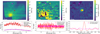 |
Fig. 1 Top: Simulation in channel 1A for a star (T = 6000 K) and a planet (T = 1000 K) separated by 1.8′′. From left to right: direct image resulting from four dithered positions, the star being offset in the bottom left corner (sum over the wavelengths of the channel); high frequencies residuals after subtracting the spectral Gaussian filter in each spaxel; correlation map with the very same template spectra as injected into the simulation for δV = 0. The red cross indicates the position of the planet, and the pink cross is the arbitrary position chosen away from the planet. Bottom: illustration of the molecular mapping technique in two spaxels, one at the position of the planet (red) and the other one at a position away from the planet (pink), for channel 1A (4.885–5.751 µm). From left to right: we display the filtering process applied to the model, the combined spectra and the Gaussian filter (black) in the two spaxels (pink and red), the high-frequency component after subtraction, and the cross-correlation function for δV= [−2000; +2000] km s−1. |
3.2 Subtracting the stellar contribution and cross-correlation
The stellar contribution in high-angular-resolution data is a mixture of the ideal diffraction pattern, and speckles due to optical aberrations, whose intensity scales with the spectrum of the star, and the phase-induced chromaticity of speckles; both scale radially with wavelength at first order. A planet buried in the diffracted halo and a star have very different spectral dependence, and can therefore be disentangled (Sparks & Ford 2002). In the IR, and in space conditions (no telluric lines), the atmospheric signature of a giant planet would appear as a high spectral frequency due to molecular absorptions, as opposed to the star contibution, which appears at a relatively low frequency. Therefore, as a prerequisite to apply the correlation with a model, the stellar contribution can be greatly attenuated by high-pass filtering, while preserving the molecular signatures of the planet spectrum almost intact (Ruffio et al. 2019). In our case, we used a Gaussian filter to suppress low frequencies on each spaxel (spectral pixel) of the cube.
We adopt a filter parameter of σ = 10, which globally maximizes the detection of the simulated planets in our sample. Prior to applying the correlation, the Exo-REM models are degraded to the maximum resolution of the MRS (3700 in the first band 1A) and are interpolated on the wavelength values of each MRS channel. The very same high-pass filter is applied to the Exo-REM models. Finally, we calculated the cross-correlation function (CCF) between the model and the data (high-pass filtered) for each velocity offset (δV) between the two spectra. Models and data spectra, which are provided at a constant δλ in MIRISim, are converted to velocity and re-interpolated to get a constant step in velocity. We used the python function scipy.signal.correlate to perform the correlation between two spectra. An example of the process in two different spaxels is shown in Fig. 1, one at the position of the planet, shown in red, and the other one at an arbitrary position, in a noise-limited region, shown in pink. The cross-correlation function shows a peak of correlation at a radial velocity of δV = 0. Looking at the spaxel away from the position of the planet, no peak in correlation is observed. We note that the MRS does not have a sufficiently high spectral resolution to resolve the Doppler shift of the known imaged planets. Therefore, no Doppler shift is included in our simulation, and we focus on the value at δV = 0 of the correlation function. The method is repeated independently on each spaxel to derive a correlation coefficient map at δV = 0 in which a planet would correspond to the highest correlation in the FoV (Fig. 1). The value of the correlation map at each of the positions i, j is given by Eq. (1), with M being the model spectra and S the spectra from the data.
 (1)
(1)
3.3 Calculations of signal-to-noise ratio
To evaluate the S/N, first Hoeijmakers et al. (2018) measured the average standard deviation of the CCF in an annulus away from the peak in correlation, and away from the position of the planet in order to avoid systematic variations in the CCF at the location of the planet due to the autocorrelation. The autocorrelation function arises from all the harmonics in the spectrum of a molecule, which produce a nonzero correlation signal away from δV = 0. For instance, the CO generates secondary correlation peaks that can be almost as strong as the main correlation peak (Fig. 2). To account for the autocorrelation, Cugno et al. (2021) added a correction. The autocorrelation function of the model spectrum is calculated and subtracted away from the peak of the CCF. However, the impact of the autocorrelation signal justifies taking into account the spatial dimension in estimating the noise. Petrus et al. (2021) measured the noise as the standard deviation of a Gaussian distribution derived from all the spaxels, excluding those containing the signal of the planet (Fig. 3). The correlation signal of the planet is averaged in the velocity space around the correlation peak and spatially in a region centered on the planet. This method is also used by Patapis et al. (2022), who measured the signal as the mean value of the CCF in an aperture centered at the position of the planet. This measurement assumes that the noise follows a Gaussian distribution, which is not always the case, depending on the instrument and on the residuals left after stellar subtraction.
These methods are also conservative, because, in principle, the signal of the planet can be integrated over several pixels. Nevertheless, measuring the S/N of a planet in the footprint of its correlation pattern is not straightforward. In Appendix B.1, we derive how the size of the correlation pattern varies at first order; we find it varies as a function of the wavelength-dependent PSF size, the template used for the correlation, and the noise level. However, the derived formula is too approximate to be used to measure the size of the correlation pattern in the data.
To obtain a robust measurement of the S/N, we defined a new method compliant with both a low level and a high level of detection and able to deal with the residual correlations of the stellar spectrum itself, which is particularly important if the temperatures of the planet and star are close, as is the case in late-type stars. Our method also accounts for the spatial variation of the noise to avoid being limited by the autocorrelation signal, as noticed in Petrus et al. (2021). Hiding the planets with a radius of 6 spaxels (maximum size of the correlation pattern estimated experimentally for a single planet in the image), we measured the noise as the standard deviation of all the other spaxels, that is, in the correlation map at δV = 0. Based on the parametric study (Sect. 4), we note that the strength of the correlation depends on the separation between the star and the planet. In addition, if the data are noisier, the correlation pattern is smaller. Finally, the width of the correlation pattern also scales with the wavelength, as does the PSF. To complement the formalism in Appendix B.1, we present more figures in Appendix B.2 to demonstrate these effects on simulated data. Concerning the astrometry, the maximum of the correlation pattern does not necessarily correspond to the real position of the planet, and this effect is more important at small angular separations. Indeed, the stellar flux can contaminate the spaxels located at the planet’s position, and so the net effect is a higher correlation value further out in the signature of the planet. Therefore, we stress that the astrometry of a companion based on the correlation map is unreliable at high noise levels and/or short angular separations. Finally, in all of our MRS simulations, we notice that the correlation pattern decreases at increasing wavelengths, especially because of a loss in sensitivity and a higher background level impacting the longer wavelengths. We also note that molecular features tend to become shallower at longer wavelengths. Given these observed behaviors, we chose to only measure the S/N in correlation maps spatially, and we define the size of the planet’s correlation pattern (containing NS spaxels) experimentally based on its radial profile. We imposed a maximum size of 6 spaxels for all channels. As a first criterion, we selected the spaxels (the red area in Fig. 4 displays a case with a higher noise level) whose correlation value is higher than three times the noise (measured in the blue area of Fig. 4). To ensure that we do not integrate noise in the signal, as the correlation pattern is not circular, we imposed a second criterion, selecting the spaxels in which the correlation is larger than 50% of the maximum correlation. In addition, to account for the particular situation where the whole profile is above 50% of the maximum correlation, which arises for example if the correlation with the star itself dominates the pattern (which is mainly the case for CO, or a hot planet around a cold star), we only use the central spaxel to measure the correlation peak. Finally, the S/N is calculated with Eq. (2), where σ is the standard deviation of the noise, and Ci the correlation values for the NS spaxels:
 (2)
(2)
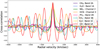 |
Fig. 2 Autocorrelation of each molecule spectrum (at T = 550 K) in the band of the spectral features. |
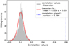 |
Fig. 3 Histogram of the pixels in the correlation map (gray area and red model), compared to the correlation coefficient at the location of the planet, as proposed in Petrus et al. (2021) and used in Patapis et al. (2022). |
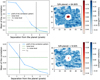 |
Fig. 4 Mean azimuthal profile of the correlation pattern (left) and typical correlation map to illustrate the S/N measurement (right), the same configuration as in Fig. 1. The pixels used to evaluate the noise as the standard deviation of the distribution are shown in blue. The pixels that are considered for the signal of the planet, as defined in Sect. 3.3, are shown in red. Top: simulation with a low noise level (example with a star at 1.8′′ from the planet). Bottom: simulation with a higher noise level (example with a star at 0.6′′ from the planet). |
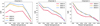 |
Fig. 5 Signal-to-noise ratio as simulated for a range of planet and star temperatures in the first three MRS channels (built over the three sub-bands). |
4 Parametric analysis of MIRI/MRS detection capacity
To evaluate the detection limit of the MRS with molecular mapping, we run two sets of simulations, and we study the impact of the spectral type and the angular separation on the detection of a planet and on the detection of each molecule included in Exo-REM. The first set of simulations (Sect. 4.1) allows us to restrain the parameter space to pursue this parametric study.
4.1 Impact of the spectral type
As the molecular mapping method relies on the fact that planetary and stellar spectra are different, we investigated the impact of the spectral type for both the star and the planet. We defined a set of 21 simulations (with a star and a planet in each simulation) by varying the planet temperature from 500 K to 2000 K in steps of 250 K, and we assumed three stellar temperatures of 3000 K, 6000 K and 9000 K, typically corresponding to M, G, and A type stars. In order to study only the impact of the spectral features, we considered a nonrealistic situation in which the stellar flux and the planet-to-star contrast are kept constant for all 21 cases. The data simulation is carried out with Ngroup = 26 and Nint = 13 for a total exposure of 1 h, which was chosen in order to achieve sufficient S/N on the planet (located at an angular separation of 1.4′′) within a reasonable computing time. The contrast at 5 µm is set to 103. The model spectrum to calculate the correlation is identical to the input spectrum.
The S/Ns measured for the three first MRS channels are displayed in Fig. 5 (similar results are observed if we look only at a single band). Globally, we find that colder planets are easier to detect with molecular mapping, as a result of molecular lines being more pronounced in the planetary spectrum. On the contrary, the hottest planet in our sample (Tp = 2000 K) features a much higher correlation with the stellar spectrum and may become almost undetectable, a feature that is even more remarkable in channels 2 and 3. These results stand regardless of the stellar spectrum, but we note that, as expected, the detection is globally poorer for a colder star, which has more spectral features (Ts = 3000 K). We also observe a general trend of a lower correlation signal with increasing wavelength, with channel 1 providing the highest detection.
4.2 Planet spectral type and angular separation
Guided by the former analysis, we chose a single stellar temperature (Ts = 6000 K) and considered more realistic simulations in which the system is located at 30 pc. Planet fluxes were calculated for the same temperature range as in Sect. 4.1 and for a radius of 1 RJup. We tested the dependency of the molecular mapping efficiency on the temperature of the planet and on its angular separation from the star. For convenience, the planet was positioned at the center of the FoV, while the position of the star was offset from 0.2′′ to 3.2′′. Compared to the simulations in Sect. 4.1, the planets here have potentially lower fluxes, and so we generated 2 h of observations with Ngroup = 33, and Nint = 19 (again with the goal being to minimize computing time).
Figure 6 displays the S/N in channels 1, 2, and 3, for each temperature of the planet as a function of the angular separation from the star. In general, the S/N does not depend only on the planet’s flux, as the continuum is filtered out while suppressing the star’s contribution, and so the high frequency is the dominant factor in the correlation. The highest S/N values are observed for temperatures ranging between 750 and 1750 K, while lower performances are obtained for the coldest (Tp = 500 K) and the warmest (Tp = 2000 K) planets because of a lower absolute flux and, respectively, a lower level of correlation due to fewer absorption lines. The S/N increases rapidly with the angular separation up to about ~l.5′′, and then becomes asymptotic (at least in channels 1 and 3). Channel 2 shows a more gradual increase in the S/N with increasing separation.
The same parametric study is performed for each individual molecule, focusing on the channel or the band in which the detection is optimal (Fig. 7). The molecules are detected in the bands for which the absorption is the largest and those departing the most from the stellar spectrum, as long as this absorption is not hidden by the absorption of another molecule. Molecules with spectral features spanning a wider range of wavelengths will benefit from calculating the S/N in the cube built over the three sub-bands of one channel.
H2O is the prominent molecule in a planet’s spectrum for any temperature. It is detected in every channel but mostly in the first one, except for cold planets where CH4 will dominate in channel 2 and hide H2O features. We observe the same trend (rapid and then asymptotic increase versus angular separation) as in the case of the full atmospheric model, although with a slightly lower S/N (120 at maximum).
CO is well detected (S/N = 10 ~ 30) for the warmest planets, from 1250 K to 1750 K (but not in the hottest one at 2000 K), and as close as 0.6−0.8′′. For colder planets at 750 K and 1000 K, CO is detectable for separations larger than 0.8′′. Because the molecule’s spectrum is featureless at wavelengths longer than 6 µm we present the result for the band 1A only, which globally presents the highest S/N. We find that the star itself produces a non-negligible correlation with CO, yielding some spatial residuals in the correlation map responsible for strong variations in the S/N curves.
CH4 is only detectable in cold planets (500 K and 750 K) in channel 2, and for separations larger than 1.4′′ as a result of fewer spectral features as compared for instance with H2O.
We note that NH3 is detected in channel 2 for planets farther than 0.8′′ and planets with T < 1000 K. The detection of NH3 will be a good tracer to discriminate between several assumptions of a planet’s temperature such as 2M1207 b (see Sect. 5.2).
PH3 and HCN have fewer features than the previous molecules; they are by nature more difficult to detect. According to the S/N analysis, we expect potential detection for the coldest objects (T < 1000 K) at rather large separations (>2′′). For PH3, we restrict the analysis to the individual band 2B and HCN in channel 3.
The abundances of each molecule as a function of planet temperature are indicated in Fig. 8, justifying the detection of NH3, CH4, HCN, and PH3 only in cold planets. For hot planets, clouds are masking the absorption lines, explaining that fewer molecular features are detected.
To provide a reference S/N, we performed the very same simulations without any star, but just a planet in the center of the FoV, which is indicated as a cross in Fig. 7. This confirms that PH3 and HCN should be detected for cold planets, in the case where the planet is not contaminated by stellar speckles. It also confirms that H2S and CO2, even if quite abundant, are not accessible to the MRS for this range of planet temperature and brightness. As for H2S, most spectral features are localized between ~5 and 8 µm, where the signature of H2O is dominating the spectrum and therefore masking H2S features. This molecule might be detectable in the case of very bright targets. The detection of CO2 is limited by shallow spectral features at 15 µm, low sensitivity of the instrument at such wavelengths, and stellar contamination. Therefore, MIRI/MRS could detect CO2 only in very bright objects, if we can manage to strongly attenuate the star’s contamination. For instance, an optimistic simulation, with a bright system at 22 pc, in which the star/planet contrast is favorable (Rstar = 0.8Rsun, Rplanet = 1.2Rjup, separation = 1.5′′), confirms this assumption: in this case, CO2 is clearly detected. None of the other molecules included in Exo-REM are detected (see Sect. 3.1). TiO has spectral features in channel 2 for the hot planets (T > 1750 K); however, it is too faint to be detected. FeH, K, VO, and Na have either no spectral features or have signatures that are too faint to be detected.
We note that for CO, CH4, and PH3, at some temperatures, the S/N of the simulation without the star is smaller than the S/N with the star. This is explained by the non-zero correlation of the star’s spectrum with these molecular features, which results in a broader correlation pattern and tends to increase the S/N. This means that the S/N calculation method is not perfect yet and could still be improved. More efficient attenuation of the star prior to applying molecular mapping could also help to reduce these effects.
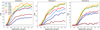 |
Fig. 6 Signal-to-noise ratio obtained as a function of angular separation from the star for a range of planet temperatures in the first three MRS channels. |
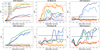 |
Fig. 7 Signal-to-noise ratio obtained at each separation from the star for a range of planet’s temperature for the following molecules H2O, CO. CH4, HCN, NH3, PH3 (in the band or channel where the spectral features are the strongest), the cross represents simulation without any star. |
Star parameters chosen for simulation.
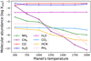 |
Fig. 8 Molecular abundance in Exo-REM models of each molecule as a function of planetary temperature. |
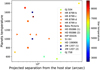 |
Fig. 9 Temperature of the planet as a function of its projected separation with its host star, for all of the planets from our sample. Stellar temperature is color coded. |
5 Molecule detection based on known systems
5.1 Choice of targets based on observational limits
To complement the parametric analysis in Sect. 4, we explored the performance with known directly imaged planets in order to estimate the relevance of future programs with JWST/MIRI. The sample was defined to fulfill observational requirements: first, the angular resolution that JWST can achieve in the mid-IR imposes angular separations of larger than ~0.3′′ (which is approximately the angular resolution for the mean MRS wavelength), and second, the sensitivity of the MRS allows us to observe targets with flux larger than 30 µJy (10 σ signal in 10 000 s, Glasse et al. 2015). Therefore, we considered the following systems: GJ 504, HR 8799, β Pic, HD 95086, HIP 65426, 51 Eri HD 106906, 2M 1207, and the brown dwarf companion GJ 758, the characteristics of which are provided in Table 3 for the stars, and Table 4 for the planets. These systems cover a broad range of temperatures, angular separations, and stellar types (see Fig. 9), and are therefore meaningful for testing our ability to characterize atmospheric parameters in the mid-IR, as compared with previous analyses in the near-IR. Furthermore, all of these planets will be observed in the GTO programs with coronagraphs, either with MIRI or NIRCam.
Stellar spectra are defined with the parameters from Table 3 and normalized to the mean flux density values at 5.03 µm5 as measured in the M band of the Johnson photometric band and tabulated at the SIMBAD astronomical database (Wenger et al. 2000). As we are studying young systems, we can expect unresolved inner dust rings to contribute to the mid-IR flux, which needs to be taken into account in the global stellar flux. Planetary spectra are generated with the Exo-REM model using a set of temperature, log g, [M/H], and C/O ratio as listed in Table 4, and their flux density is scaled to the distance of the system and the planet’s radius. For some systems, the flux level is adapted so that the models globally match the near-IR data. These data are then converted to MIRISim input requirements: µJy for the flux density, and µm for the wavelengths. We used http://whereistheplanet.com (Wang et al. 2021) to infer the astrometry of the planet for an arbitrary date of June 2023 (likely the start of JWST cycle 2). For long-period planets, their projected positions do not vary significantly with the date (except for β Pictoris b).
The position and the spectrum of each object are used in the Exposure Time Calculator (ETC) to calculate the observational parameters (Ngroup, Nint). The number of groups per integration Ngroup was determined to avoid saturation while maximizing counts. We then chose the number of integrations to reach an S/N of higher than 3 (and ideally above 5) on the detector for the planet’s flux in each spectral band for the complete observation. The S/N is extracted on an aperture of 0.4′′ centered on the planet. These parameters are indicated for each simulation in Table 5. The ETC also provides a convenient way to check that the planet is contained within the FoV, based on the astrometry. When needed, we adapted the telescope pointing, either to position the planet at a suitable location on the detector (especially if the angular separation is of the order of the size of the FoV) or to move away from a bright star that might cause saturation and latency. The S/N of the detection for each molecule of each system is provided in Table 6.
Parameters of the simulated planets.
Simulation parameters for each target.
5.2 Simulations and molecular mapping analysis of this planet sample
GJ 504 b is a T8-T9.5 object discovered by (Kuzuhara et al. 2013). Bonnefoy et al. (2018) analyzed the system in detail in order to constrain its atmospheric parameters with near-IR data (from 1 to 2.5 µm). The uncertainty on the age (21 Myr to 4 Gyr) of this system gives two mass regimes (1 Mjup or 23 Mjup), making this object either a young exoplanet or an older brown dwarf. More measurements on the molecular abundances and metallicity are needed to put more robust constraints on the planet and thus on its formation. Methane has been detected in the atmosphere of this planet by Janson et al. (2013), but no other molecular feature has been detected yet.
The system is simulated by offsetting the star outside of the FoV at coordinates (2.0, –2.5)′′. As it is a nearby system, the star is too bright for the MRS and the detector would saturate in a few groups. Offsetting the star allows longer integrations. Processing the simulated data with the molecular mapping method, we obtained the correlation maps shown in Fig. 10, which displays the S/N for each detection. We were able to detect H2O, CO, CH4, NH3, HCN, and PH3. Moreover, the correlation with the full model allows the detection of wavelengths up to 18 µm (Fig. C.11).
As a test case, we ran the simulation without the star to assess the impact of the stellar contribution. We find an improvement of the S/N by a factor of three for NH3 and HCN, respectively, and by a factor of two for CH4. Other molecules are also easier to detect, and in particular, an S/N = 6.8 is achieved for CO2. These results argue for better stellar removal to improve the detections and possibly detect CO2 in this system and other similar systems.
The HR 8799 system harbors four young giant planets with similar characteristics in terms of temperature and luminosity. These planets were discovered by Marois et al. (2008, 2010). The presence of a planetesimal belt was inferred from submillimetric observations with ALMA (Booth et al. 2016). Water and carbon monoxide were clearly identified at high S/N in HR 8799 b, c, and d (Petit dit de la Roche et al. 2018; Barman et al. 2015; Ruffio et al. 2021). However, the presence of methane is still debated; in the case of HR 8799 b, it was claimed by Barman et al. (2015) using cross-correlation with a model spectrum on Osiris Keck data, but this was not confirmed using molecular mapping on the same data (Petit dit de la Roche et al. 2018) or with complementary data (Ruffio et al. 2021). Broadband photometry of planets b, c, and d has provided evidence of significant atmospheric cloud coverage, while spectroscopy of planets b and c shows evidence for nonequilibrium CO/CH4 chemistry (Janson et al. 2010; Hinz et al. 2010).
In the Simulation, the star is offset to the coordinates (−0.4, 0.0)′′ from the center of the FoV to be sure that all four planets are contained in a single dither position. The planet e cannot be detected, as it is too close to the star to be resolved with the MRS. The correlation maps of these simulated data are displayed in Fig. C.1. We detect H2O and CO (for planets b, c, and d). There is also a faint detection of NH3 and CH4 for planet b. No other molecule is detected.
The β Pictorís system has two discovered planets Lagrange et al. (2009, 2010, 2019); Nowak et al. (2020a). Planet c is too close to the star and cannot be resolved with the MRS; therefore we focus on planet b. This planet has a dusty atmosphere (Bonnefoy et al. 2013). Water and carbon monoxide were detected in its atmosphere with SINFONI data using molecular mapping (Hoeijmakers et al. 2018). Using the observation parameters of the GTO 1294 (PI: C. Chen), we did not manage to detect the planet. Therefore, we chose to increase the number of integrations. From the angular separation and temperature of the planet, we do not expect a strong detection. However, the brightness of the target still allows us to detect the planet with the full atmospheric model, while H2O is the only detected molecule. The correlation maps corresponding to this system are presented in Fig. C.2.
HD 95086 b was detected by Rameau et al. (2013), who showed that it has a cool and dusty atmosphere, where the effects of possible nonequilibrium chemistry, reduced surface gravity, and methane bands in the near-IR might be explored in the future. Chauvin et al. (2018) found that its near-IR spectral energy distribution is well-fitted by spectral models of dusty and/or young L7-L9 dwarfs. Here, we aim to test the two scenarios highlighted in Desgrange et al. (2022) using SPHERE observations combined with archival observations from VLT/NaCo and Gemini/GPL These scenarios indicate that the color of the planet can be explained by the presence of a circumplanetary disk around planet b, with a range of high-temperature solutions (1400–1600 K) and significant extinction, or by a super-solar metallicity atmosphere but lower temperatures (800–1300 K), and a small to medium amount of extinction. We performed two simulations, one with a planet at the temperature of 800 K and a second with a planet of 1400 K. With the full spectrum, the planet is only detected in the coldest scenario. In terms of molecules, we secured the detection of H2O, but marginally detect NH3. These results are presented in Fig. C.3 for the cold planet scenario and in Fig. C.4 for the warm planet scenario. The planet is close to its star (one of the closest in our sample) and this system is located at a large distance, which explains the globally faint detection of the planet and nondetection of other molecules.
HIP 65426b was discovered by Chauvin et al. (2017) with VLT/SPHERE. The Y- to H-band photometry and low-resolution spectrum indicate a L6 ± 1 spectral type and a warm, dusty atmosphere. Petrus et al. (2021) studied this system with different methods, including molecular mapping using VLT/SINFONI data and detected carbon monoxide and water vapor. The planet is detected in channel 1, and only the molecule H2O is detected. At this temperature, the detection of CO was expected from our parametric study. However, in the case of this system, which is almost four times more distant than the systems simulated in the parametric studies, the fainter flux of the planet explains why we do not have better detection of the planet and no detection of CO.
51 Eri b was discovered with GPI in the near-IR. Macintosh et al. (2015) indicates that it has a T4.5-T6 spectral type and the J-band spectroscopy shows methane absorption. From VLT/SPHERE data in the near-IR, Samland et al. (2017) derived the presence of vertically extended, optically thick cloud cover with small particles. 51 Eri is a bright star, therefore the number of groups is small, allowing saturation to be avoided and integration time is larger than for other sources in order to achieve the S/N required to detect the planet. The correlation maps are shown in Fig. C.6. Even though the planet is bright, it is not detected as it is too close to the star to be observable with this method, as expected from our parametric study in Sect. 4.
HD 106906 b is a young low-mass companion near the deuterium burning limit (Daemgen et al. 2017). It has been characterized spectrally in the near-IR with VLT/SINFONI. This planet is the hottest and the most distant from its star in our sample. Therefore, to simulate this system, we chose to have the planet in the center of the FoV and the star’s PSF located outside the FoV. In principle, molecular mapping is not required to detect the planet as it is far from its host star and sufficiently bright. Applying molecular mapping, the planet is detected in all three channels, and we are able to detect H2O and CO. At high temperatures, we do not expect other molecules to be detected, as we can see in Fig. C.7.
2M 1207b was the first planet ever detected with direct imaging by Chauvin et al. (2004) and will be one of the first exoplanets targeted with the MRS (GTO 1270, PI: Stephan Birkmann). The atmospheric properties of 2M 1207 b are not well constrained, and the MRS observations have the ability to break the degeneracy between two radically different models. On the one hand, Barman et al. (2011) proposed a temperature of 1000 K, log(g) = 4 and 1.5 RJup which is in agreement with the first estimate of Chauvin et al. (2004); on the other hand, Patience et al. (2010) found a best-fit model at about 1600 K and log(g) = 4.5 with a smaller radius of 0.5 RJup.
The correlation maps are shown in Figs. C.8 and C.9. Considering the model at 1000 K, we obtained detections of H2O, CO, and NH3. The planet is detected at a very high S/N with the full model. For the model at 1600 K, the detection of H2O is much weaker and CO is undetected simply because the planet is smaller than in the former case. NH3 is also undetected, as expected for such a high temperature based on the parametric study. The star being an M8 brown dwarf, the warmer planet scenario represents an extreme case for the molecular mapping method; but based on our simulations, the MRS has the ability to provide a definitive answer regarding its temperature. The detection of NH3 can be a good indicator of the temperature of the planet.
GJ 758 B is a brown dwarf companion to a solar-type star. It was discovered with Subaru/HiCIAO (Thalmann et al. 2009) and characterized with VLT/SPHERE in Vigan et al. (2016). No atmospheric model perfectly reproduces the measured fluxes of GJ 758 B in the near-IR. As one of the coldest companions to have been directly imaged, it also appears to be an interesting target to apply molecular mapping. The star is bright, and therefore we offset it outside the FoV at coordinates (2.3, 1.3)′′, and we used Ngroup = 59, and Nint = 5 for a total exposure time of 3374.45 s for one observation. The dithering pattern is modified from the default pattern to be optimized for the system. Correlation with the full spectrum yields a detection in the three channels, while both H2O and NH3 are clearly detected, and CH4 can be suspected. These results are displayed in Fig. C.10.
S/N detection measured in correlation maps with the full atmospheric model and molecules templates for each planet of the sample.
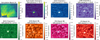 |
Fig. 10 Example of correlation maps for the simulated system GJ 504 with Exo-REM full atmospheric template and molecular template. Each molecule is shown in the channel or band where the S/N is the highest. |
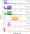 |
Fig. 11 Exo-REM molecular template spectra of GJ 504 b. The parts of the spectra corresponding to the channels or bands shown in Fig. 10 are highlighted. |
6 Atmospheric characterization using grids of Exo-REM models for GJ504 b
The results presented in the former section suggest that GJ 504 b is the most interesting target of our sample for molecular mapping with the MRS. Here, we explore the potential for characterization of this specific system using two methods: one based on the correlation maps and the other on χ2 minimization.
6.1 Correlation maps with a grid of models
After subtracting the low frequencies on data and models spectra (same method as in Sect. 3.2), the data are correlated with a grid of Exo-REM models, varying the temperature, the metallicity, the surface gravity, and the C/O ratio of the models. Models are high-pass filtered in the same way as the data. For each model, we calculate the correlation map with the correlation coefficients using Eq. (3), where σS(λ) is the uncertainty on the flux at each wavelength, as extracted from the ERR extension of the cubes (see Sect. 2.3). This value takes into account the photon noise and detector noise in each spaxel.
 (3)
(3)
Figure 12 shows the grids of correlation with the correlation value at the position of the planet, which we obtained when exploring two parameters at once. In practice, for each coordinate in any of the grids, corresponding to a couple of parameter values, we took the maximum correlation coefficient obtained when varying the two other parameters. The real parameters of the planet provided as input to the simulation are indicated with black crosses.
In general, a significant range of models produce high correlation values, resulting in a broad peak around the input parameter values, which implies a relatively low accuracy on the retrieved parameters. Still, the C/O-versus-temperature correlation grid matches the input parameters reasonably well (bottom subplot in Fig. 12). On the contrary, we observe a tendency for higher metallicity and higher surface gravity in the two upper subplots of Fig. 12. This apparent mismatch is discussed in the following section.
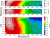 |
Fig. 12 Grids of the correlation coefficient between the spectrum at the position of the planet and the Exo-REM models. Case of GJ 504 in channel 1. Similar results are observed for the other bands or reconstructed channels. |
6.2 χ2 minimization with a grid of models
The method described in Sect. 6.1 based on the correlation with models is not sufficient to evaluate the reliability of the best model (maximum correlation) with respect to the data. In addition, the noise estimation does not take into account the spatial noise induced by speckles. We now investigate the characterization capabilities using χ2 minimization. Starting from the high-frequency spectrum extracted at the position of the planet, we compare it to the same grid of high-pass filtered Exo-REM models. We use the correlation map to define where the planet is located, and then extract a high-frequency spectrum in the cubes after the high-pass spectral filtering on the spaxels. We extract that spectrum for the signal of the planet by co-adding the flux in the spaxels that are defined by the S/N analysis (Sect. 3.3).
We note that this high-frequency spectrum does not contain any information on the total flux of the planet because of the subtraction of low frequencies. We introduced a factor R, which is chosen to minimize the χ2 for a given model, as given in Eq. (5). This factor corresponds to a global scaling parameter that does not influence the shape of the synthetic spectra, but allows us to take into account the planet’s radius (as done in Baudino et al. 2015), and also captures some photometric calibration issues between the MIRISim simulated model and the actual model.
For each model, we determined the χ2 using Eqs. (4) and (5), in which σF(λ) is the uncertainty on the flux measured at each wavelength in an annulus at the same planet’s separation from the star in the high frequencies cubes. The noise σs extracted from the JWST pipeline is now negligible, and this noise σF takes into account the spatial variation in the high-frequency cubes. Similarly to Fig. 12, we display the  values of the grid of models in Fig. 13.
 (4)
(4)
 (5)
(5)
As a sanity check, we obtained χ2 values that are in agreement with the number of independent points in the spectrum. The χ2 minimization gives similar results compared to the grid of correlation values. Again, several models yields χ2 values that are close to that of the input model, although the 1σ, 2σ, and 3σ contours point to a more restrained region in the C/O-versus-temperature grid when compared to Fig. 13. However, this is not the case for the metallicity and the surface gravity; these parameters are not well constrained, which is likely due to degeneracies between them. Indeed, the metallicity and the surface gravity information are mostly contained in the relative depth of the lines, which are affected by the filtering stage. It is therefore more difficult to disentangle two models that have different metallicity or surface gravity values. On the contrary, the abundance of molecules, such as H2O, CO, and CH4, which define the C/O ratio, depends on the temperature of the planet. Even though the continuum of the planetary spectrum is lost in the filtering, they still have a net effect in the high-frequency spectrum of the planet, explaining the relatively good match obtained for the temperature and the C/O ratio. In the event that one of these parameters is well determined by other methods or other observations, the remaining parameters can be well constrained with high confidence, as illustrated in Fig. 14, in which the surface gravity is fixed at the input values (log ɡ = 4.0) in each subplot.
7 Discussion
In this section, we discuss qualitatively various aspects of the molecular mapping technique applied to MIRI/MRS, in particular, the advantages and disadvantages, as well as possible improvements, and the complementary with other observing modes and instruments.
7.1 Pros and cons of the mid-1 R for the molecular mapping
The mid-IR spectral range offers advantages when combined with molecular mapping with respect to the near-IR. For instance a planet at 700 K has its emission peak at 5.2 µm while the stellar contribution becomes less dominant at longer wavelengths. According to the parametric study (systems at 30 pc, planets of 1 Rjup around a star at 6000 K, 2 h per observation), the MRS should allow us to detect planets at separations of greater than 0.5″ (except the hottest planet around the coldest star in our sample) and to characterize those that are further away than 1″ from their star. We find that planets with temperatures above 500 K and below 1500 K will be easier to detect, especially if they orbit G-type stars or younger. In addition, the mid-IR gives access to molecules that are not easily accessible at shorter wavelengths because of fainter absorption features (such as NH3, HCN).
On the contrary, the angular resolution is lower than in the near-IR, and so stellar contamination becomes a more important issue. For this reason, we chose GJ 504 b to perform a detailed characterization study as it features favorable configurations in terms of angular separations and temperature. The comparison to a grid of models with χ2 approach provides reasonable results (Sect. 6) but for other targets that are too close to their star, the confidence regions in the χ2 maps are too large to reduce the accuracy on the atmospheric parameters. Only planets with S/N larger than 30 in our sample (HR 8799 planets, 2M 1207 b at 1000 K) are amenable to atmospheric characterization with the MRS. We note that the extracted spectra of the others planets (with S/N < 30) are too contaminated by stellar residuals. Although well detached, HD 106906 b is a special case because Exo-REM is not well adapted to modeling a planet at this temperature; other atmospheric models would therefore be needed to characterize this planet.
Moreover, having priors on the atmospheric parameters to correlate our data with models is necessary to reduce the explored parameter range. As a first approximation, one can use the high-frequency spectrum before applying the molecular mapping in order to restrain this range using the χ2 minimization. While we will benefit from the use of both analyses, namely molecular mapping and χ2 minimization, other methods of atmospheric retrievals would be relevant to study these planets further.
Finally, molecular mapping relies on the fact that the spectrum has lots of spectral features due to the molecular absorption and might be less efficient for young dusty planets, as dust and clouds tend to flatten the spectrum, as noted for the PDS 70 planets in Cugno et al. (2021) (extinction due to dust has not been taken into account in the present work). Further works should be continued to test the impact of clouds and extinction on molecular mapping.
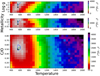 |
Fig. 13 Values |

 |
Fig. 14 Values |

7.2 Possible improvements in the data reduction and molecular mapping
As a source of problems for the characterization, stellar subtraction should be tackled with more efficient methods, especially for planets located at separations of below 1″, which are more affected by the starlight. Subtracting a scaled template from each spectrum in the data cube as in Hoeijmakers et al. (2018) gives a slightly higher S/N for the detection of the planets closer than 1″ (such as ß Pictoris b) but shows no improvement for more distant targets. As we noted from the ideal simulations with no star in the scene, and providing that the photon noise and the speckle noise are below the background noise, a significant improvement of the S/N is possible for the most impacted molecules (NH3, CH4, HCN, CO2), which highlights the potential benefit of developing more efficient PSF subtraction algorithms. Consequently, more targets would be accessible for characterization with the MRS and molecular mapping. Other interesting targets might come from future ground-based surveys, such as The Young Suns Exoplanet Survey (Bohn et al. 2020), and SHINE with VLT/SPHERE (Vigan et al. 2021).
A second avenue for improving the performance of molecular mapping with MIRI is to take advantage of the full spectral range. Hitherto, because of current limitations in the pipeline, we have restrained the method to the MRS channels, but exploiting the full spectral range of MIRI should increase the detection of molecules that exhibit features at multiple wavelengths in different channels (such as NH3). Two solutions are envisioned, either a full concatenation of the data cubes from each channel or the extraction of the planet spectrum channel per channel, prior to cross-correlation with the model. The first method is limited by interpolation artifacts while the second one requires the planet to be detected in each of the three channels.
7.3 Interpretation of the detection of the molecules in the targets sample
All planets in our sample except 51 Eri b – for which it is too challenging to disentangle the planet signal from that of the star – are detected using the correlation with a full atmospheric model. Depending on the distance of the system, long integrations (more groups) are possible, effectively improving the ramp fitting. However, the planets are fainter if more distant, meaning that longer exposure times are required (more than 4 h per observation for HD 95086). In contrast, bright stars like ß Pic and 51 Eri impose fewer groups per integration, which has a definitive impact on the planet detection, while at the same time the angular separation is smaller than 0.5″, meaning that the star cannot be moved out of the FoV.
The planet GJ 504 b, although being the target with the largest contrast with its star, is the target with the highest S/N. On the contrary, 2M 1207 b is the one with the lowest contrast (in both temperature hypotheses) but its detection is much weaker. The S/N is eight times higher for GJ 504 b than for 2M 1207 b if the planet is at 1600 K.
We note that H2O, the most abundant molecule in the atmosphere of giant planets and also the one with the most numerous spectral features, is always detected, even in planets that are close to their star and thus heavily contaminated by the starlight (β Pic b, HD 95086 b, HIP 65426b). H2Ois the only molecule unambiguously detected in these systems. This result is consistent with the parametric study; it is even detected with a slightly higher S/N than the correlation with the full atmospheric model, which can be explained by the fact that H2O does not correlate with stellar residuals, contrary to the full atmospheric model. CO is the second-most abundant molecule in most planets of the sample. However, it is detected only for planets with separations larger than 0.8″. Indeed, as confirmed by the parametric study, CO is the molecule that suffers the most from stellar contamination, which also explains its nondetection when the planet has a low flux (such as HIP 65426, although it is at 0.8″ and 2M 1207 b at 1600 K with the small radius hypothesis).
On the contrary, PH3 and HCN are among the least abundant molecules, but their spectral features are such that they can be detected in cold planets, providing that they are bright (nearby and well-separated, as in the case of GJ 504 b), in agreement with the parametric study.
The access to these molecules is a unique feature of JWST observations as it allows us to derive new constraints on planetary atmospheres as well as on planet formation. In complement to NIRSpec data, which can access the bright features of PH3 around 4.3 µm, we show that MIRI/MRS can also detect or confirm the presence of this molecule. Mukherjee et al. (2022) showed the importance of PH3 in the emission spectrum of an atmosphere in thermochemical disequilibrium (based on MIRI-LRS simulations). Furthermore, measuring the phosphine abundance, which is the dominant phosphorus molecule, can provide an estimation of the P/O ratio. These abundance ratios are of interest for determining whether or not an element is depleted compared to oxygen, which provides valuable information on the planet-formation processes. In addition, Zahnle & Marley (2014) details the importance and implications of NH3, CH4, and HCN in the atmospheres of young giant planets and brown dwarfs. These molecules are key to accurately deriving the C/O and N/O ratios, all being accessible to the MRS. They could also be indicators of chemical disequilibrium and provide constraints on the deep atmospheric temperatures and strength of vertical mixing that characterize the so-called “quench level”.
NH3 is also a powerful indicator of both planetary effective temperature and atmospheric chemical equilibrium state. Differences between two model spectra calculated at equilibrium and disequilibrium chemistry arise between 5 and 9 µm. These differences mainly arise from different CH4, H2O, and NH3 abundances due to differences in the quench level (Mukherjee et al. 2022).
7.4 Influence of the atmospheric models
The molecules that are detected with molecular mapping are clearly closely related to the atmospheric model used to generate the templates. This explains some differences in the case of HR 8799 and GJ 504 with Patapis et al. (2022), who used the petitRADTRANS model. In the analysis of these latter authors, CO is not detected in GJ 504 b. Indeed, their molecular abundances computed with petitRADTRANS show significant differences from values computed with Exo-REM (e.g., lower CO abundance for a planet at 550 K). Similarly, in the case of the HR 8799 system, Patapis et al. (2022) obtained a higher detection of CO for planet c than for planet b, the former having a higher temperature and therefore more CO according to petitRADTRANS compared to the findings of Exo-REM. In addition, CH4 are less abundant in Exo-REM-based models with respect to models from petitRADTRANS, which explains why the detection of CH4 is lower in our analysis of the HR 8799 planets. These differences in molecular composition mostly come from a different treatment of the chemistry. In Exo-REM, chemical abundances are computed assuming chemical disequilibrium with quenching levels (generally between 1 and 10 bar) derived from a parametrization of the vertical mixing. In contrast, in Patapis et al. (2022), the quenching level is fixed at 10−1 bar and assumes equilibrium chemistry.
Also, we can expect a family of models that best fits the ground-based near-IR data to show large differences in the mid-IR regime. Depending on model assumptions, there is a large range of atmospheric parameter values that can reproduce the data. Therefore, the simulations presented in this paper should not be considered a perfect reproduction of each target, as long as we currently have little or no constraint in the mid-IR range for the known directly imaged planets.
7.5 Complementarity with MIRI coronagraphy
Although molecular mapping is a powerful tool for identifying the presence of molecules, it has difficulty putting meaningful constraints on atmospheric parameters, as long as the planet continuum is significantly affected by the first step, in which the stellar contribution is subtracted. In that respect, complementary observations would be useful, in particular those with MIRI’s coronagraphs, which are observing in the same spectral range as the MRS but with specific wavelengths and broader bandwidths. The 4QPM coronagraphs (Boccaletti et al. 2015) can provide photometric measurements of the continuum flux (11.4 µm and 15.5 µm) of a planet, as well as the NH3 feature at 10.65 µm, which are certainly useful for providing priors for the MRS data analysis. The combination of observations with the MRS and the coronagraphs will be decisive in further constraining the atmospheres of known directly imaged planets as illustrated in Danielski et al. (2018).
7.6 Complementarity with future ground-based projects
MIRI/MRS has the advantage of not being impacted by telluric lines in comparison to the data taken with ground-based instruments. Still, future ELT instruments are highly complementary to the MRS in providing higher spectral resolution and different wavelength coverage.
In the near-IR, HARMONI allows a range of spectral resolution settings (3000, 7000, 18 000). Houllé et al. (2021) simulated molecular mapping observations combined with a matched-filter approach, showing that planets with contrasts of up to 16 mag and separations of down to 75 mas can be detected at >5σ.
In the mid-IR, METIS provides high-resolution spectro-imaging (R~ 100 000) at L/M band, including a mode with extended instantaneous wavelength coverage (assisted by a coro-nagraph). Snellen et al. (2015) showed that an Earth-like planet orbiting αCen could be detected at a S/N of 5 with an instrument like METIS. We note that the METIS M band overlaps with the shortest wavelength of the MRS.
8 Conclusions
In the following, we summarize the main specific conclusions of our study.
As already showcased in Patapis et al. (2022), we confirm that the MIRI/MRS mode has the potential to enhance planet detection owing to the molecular mapping technique which performs cross-correlation with atmospheric models.
To determine the significance of the detection, we propose a data-driven experimental method, which takes into account the size and the shape of the correlation pattern in order to avoid the impact of the autocorrelation that arises for molecules that have harmonics in their spectra. While satisfactory for a majority of cases, the S/N may be overestimated in particular situations: with a CO template, or either with a hot planet (T = 1000 K) around a cold star.
The correlation pattern differs from a PSF and scales with the wavelength at a high S/N but also depends on the strength of the correlation, the atmospheric template, and the noise level. Importantly, the maximum of the correlation pattern does not necessarily correspond to the real position of the planet (stronger effect at small angular separations). As a result, astrometry is unreliable with correlation maps.
From the parametric study, which samples a range of planetary temperatures and angular separations, we concluded that, while planets are detected as close as 0.5″, a good level of characterization requires more angularly separated objects, typically larger than 1″. The stellar spectral type has little impact on the performance, as opposed to the temperature of the planet. The highest S/N values are achieved for planet temperatures ranging between 750 and 1750 K, while lower performances are obtained for the coldest (Tp = 500 K) because of a lower absolute flux, and the warmest (Tp = 1000 K) planets because of a lower level of correlation due to fewer spectral features.
For planets typically colder than 1500 K, the following molecules are detectable: H2O, CO, NH3, CH4, HCN, PH3, and CO2. Some of these molecules have never been confirmed or even detected in the atmosphere of an exoplanet.
We propose three directions for improving the performance of the molecular mapping method with MIRI. Firstly, further exploring the subtraction of the stellar contribution could allow the detection and characterization of planets closer than 1″ as well as the detection of the molecules that have less spectral features or that are more hidden by other molecules. Secondly, a robust estimation of the S/N would require developing a more sophisticated analytical approximation to model the size and shape of the correlation pattern. Finally, we plan to perform a Bayesian analysis in order to better constrain the atmospheric parameters and to better evaluate the uncertainties of each parameter.
Complementary data, such as coronagraphic mid-IR photometry with MIRI, for measuring the planet continuum will provide temperature and surface gravity estimates, which in turn can be taken as constraints on the atmospheric parameters for characterization purposes using molecular mapping.
Interpretation of the data processing with molecular mapping strongly depends on the assumptions of the models used to generate synthetic spectra. A pilot program dedicated to a specific target will represent a benchmark for systematically comparing several models.
In this paper, we show that future JWST observations with MIRI-MRS are capable of providing a clear detection of molecules in the atmospheres of young giant planets, which is key to measuring abundance ratios and ultimately providing constraints on their formation and evolution.
Acknowledgements
M.M. acknowledges the Centre National d’Études Spatiales (CNES, Toulouse, France) for supporting the Ph.D. fellowship. B.C. and B.B. acknowledge financial support from the Programme National de Planétologie (PNP) of CNRS/INSU. This work was granted access to the HPC resources of MesoPSL financed by the Région Île-de-France and the project Equip@Meso (reference ANR-10-EQPX-29-01) of the programme Investissements d’Avenir supervised by the Agence Nationale pour la Recherche. This project has received funding from the European Research Council (ERC) under the European Union’s Horizon 2020 research and innovation programme (COBREX; grant agreement no. 885593; EPIC, grant agreement no. 819155). This publication makes use of data products from the Wide-field Infrared Survey Explorer, which is a joint project of the University of California, Los Angeles, and the Jet Propulsion Laboratory/California Institute of Technology, funded by the National Aeronautics and Space Administration. The results presented in this research paper were obtained using the python packages numpy (Harris et al. 2020), scipy (Virtanen et al. 2020), matplotlib (Hunter 2007) and astropy (Astropy Collaboration 2013, 2018).
Appendix A JWST pipeline
Stage 1. The first stage of the pipeline corrects for the detector effects. The input raw data are in the form of one or more ramps (integration) containing accumulating counts from the nondestructive detector readouts. The output is a corrected count-rate (slope) image. Corrections are applied group by group: first, the pipeline corrects the quality of the pixels, flagging those that will not be used. The step dq_init initializes the data quality using a reference file where known bad pixels are indicated. Saturated pixels are flagged with the step saturation. The first and the last groups of each integration are suppressed as they are the most affected by detector effects (firstframe, lastframe). The linearity step applies for each pixel a correction for the non-linear detector response, using the “classic” polynomial method where the coefficients of the polynomial are stored in a reference file. Dark current is corrected by subtracting dark current reference data from the input science data model (dark). On each integration ramp within an exposure, we perform cosmic rays/jumps detection (jump) by looking for outliers in the up-the-ramp signal in each pixel. Finally, ramp fitting determines the mean count rate in units of counts per second for each pixel by performing a linear fit to the data in the input file (ramp_fitting). This stage 1 takes 4D data in the shape of (Nint, Ngroup, Npixel,x, Npixel,y) to 2D images for the detector (Npixel,x, Npixel,y). Other steps of corrections are available but they will not be useful for simulated data, and will be considered for the real on-orbit data.
Stage 2. The second stage of the pipeline corresponds to the calibration, and includes additional corrections depending on the instrument and the observation mode to produce fully calibrated exposures. First, the pipeline associates a WCS object with each science exposure, which transforms the positions in the detector frame to positions using the International Celestial Reference System (ICRS) frame and wavelength (assign_wcs). The Source Type (srctype) step attempts to determine whether a spectroscopic source should be considered a point or extended object. Fringes in spectra are corrected (fringe). Finally, photometric calibrations allow count rates to be converted into surface brightness (in MJy/str) (photom). The outputs are 2D calibrated data of the detector.
Stage 3. The last stage is intended for combining all calibrated exposures. We can also subtract or equalize the sky background in science image (mrs_imatch). Outliers, bad pixels, and cosmic rays that would remain are flagged using the outlier_detection step. This stage takes into account the different dither positions to build a data cube with cube_build and extract a spatially averaged spectrum over the full field of view with extract_1d. We can choose to construct cubes for each band or combine bands and channels with a larger wavelength range. The outputs are 3D cubes with two extensions, the SCI image contains the surface brightness of the spaxels, and the ERR image is the uncertainty of the SCI values.
Appendix B Size and shape of the correlation pattern in a simple case
Appendix B.1 Analytical first approximation
To have an idea of the parameters involved in the correlation that should help to understand the size of the correlation pattern, we derive a formula for the correlation depending on its parameters. We defined S as the observed spectrum and M as the model spectrum. The noise in the observed spectrum is is ξ ~ 𝒩(0, ξ(λ)), and P is the PSF.
 (B.1)
(B.1)
The correlation can be written as
 (B.2)
(B.2)
The numerator can be written as
 (B.3)
(B.3)
 (B.4)
(B.4)
 (B.5)
(B.5)
More specifically, the norm of the observed spectrum is
 (B.6)
(B.6)
 (B.7)
(B.7)
Finally,
 (B.8)
(B.8)
If the PSF function Px(λ) is a Gaussian Gσ(x) with x the spaxel distance from the centroid and with a wavelength-dependent width σ(λ)=σ0λ/λ0, then we may develop P at first order in (λ − λ0)/λ0 as
 (B.9)
(B.9)
 (B.10)
 (B.11)
In the following, we write  .
.
The different terms in the numerator and in the denominator involving Px(λ) can be developed according to the above equation at first order in (λ − λ0)/λ0. Linearizing all first-order terms leads to the following equation:
 (B.12)
where we define:
 (B.13)
 (B.14)
The parameter δ2 can be considered as a positive constant that depends on the S/N level in the cube, while ß can be bounded by the wavelength range of the considered channel. Indeed, as λmin< λ < λmax,
 (B.15)
Therefore, since the channel windows are on the order of λ0±l4 − 18%, we expect ß<0.18. The zeroth-order term  is therefore a good approximation of the correlation pattern, and ndicates that the correlation pattern will depend on the PSF, but also on the model spectrum and on the noise. However, this formula is insufficient to estimate a correlation radius, and would result in an oversized correlation pattern. Indeed this is correct in the case of data dominated by Gaussian noise, which is not the case at long wavelengths and when we have more stellar residuals. It also assumes that the PSF is a Gaussian.
Appendix B.2 Example of simulations from the parametric study
Simulations show that we obtain different shapes and sizes of the correlation pattern depending on the noise level and the molecules studied. Figure B.1 presents correlation maps for a planet at 500 K; it is a comparison between the direct image and the correlation maps for three detected molecules (NH3, CH4, and PH3) at the same wavelength (band 2B) and same star–planet separation. Figure B.3 and Fig. B.4 is a comparison between CO and H2O for four values of separation between a star and a planet. This corresponds to the simulation with a planet at 1750 K, in band 1A. Moreover, it is notable that astrometry is unreliable, mostly for short star-planet separations. The asymmetry of the correlation pattern is clearly visible in Fig. B.3. Concerning the mean azimuthal profile, we note that the profile of the PSF is unchanged regardless of the noise level, whereas the profile of the correlation pattern depends on the noise level and on the template with which we correlate the data.
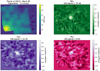 |
Fig. B.1 Simulations from the parametric study with the planet at 500 K and the star separated at 3.2″. Correlations maps with different molecular templates: NH3, CH4, and PH3 in the band 2B. |
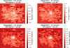 |
Fig. B.3 Simulations from the parametric study with the planet at 1750 K and the star at different separations. Correlation maps with CO in band 1A. |
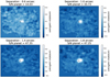 |
Fig. B.4 Simulations from the parametric study with the planet at 1750 K and the star at different separations. Correlation maps with H2O in band 1A. |
Appendix C Simulations and correlation maps for each planet
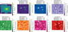 |
Fig. C.1 MIRISim simulation and correlation maps of the simulated system HR 8799. |
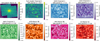 |
Fig. C.2 MIRISim simulation and correlation maps of the simulated system ß Pictoris. |
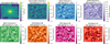 |
Fig. C.3 MIRISim simulation and correlation maps of the simulated system HD 95086 at 800 K. |
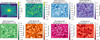 |
Fig. C.4 MIRISim simulation and correlation maps of the simulated system HD 95086 at 1400 K. |
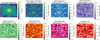 |
Fig. C.5 MIRISim simulation and correlation maps of the simulated system HIP 65426. |
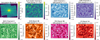 |
Fig. C.6 MIRISim simulation and correlation maps of the simulated system 51 Eri. |
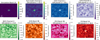 |
Fig. C.7 MIRISim simulation and correlation maps of the simulated system HD 106906 the simulation plot shows the planet directly (in the center). |
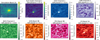 |
Fig. C.8 MIRISim simulation and correlation maps of the simulated system 2M 1207 at 1000 K. |
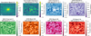 |
Fig. C.9 MIRISim simulation and correlation maps of the simulated system 2M 1207 at 1600 K. |
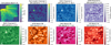 |
Fig. C.10 MIRISim simulation and correlation maps of the simulated system GJ 758. |
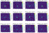 |
Fig. C.11 MIRISim simulation and correlation maps of the simulated system GJ 504 for the three first channels. The scale is the same in each band and channel. |
References
- Astropy Collaboration (Robitaille, T. P., et al.) 2013, A&A, 558, A33 [NASA ADS] [CrossRef] [EDP Sciences] [Google Scholar]
- Astropy Collaboration (Price-Whelan, A. M., et al.) 2018, AJ, 156, 123 [Google Scholar]
- Barman, T. S., Macintosh, B., Konopacky, Q. M., & Marois, C. 2011, ApJ, 735, A39 [Google Scholar]
- Barman, T. S., Konopacky, Q. M., Macintosh, B., & Marois, C. 2015, ApJ, 804, 61 [Google Scholar]
- Baudino, J.-L., Bézard, B., Boccaletti, A., et al. 2015, A&A, 582, A83 [NASA ADS] [CrossRef] [EDP Sciences] [Google Scholar]
- Birkby, J. L., de Kok, R. J., Brogi, M., et al. 2013, MNRAS, 436, L35 [Google Scholar]
- Blain, D., Charnay, B., & Bézard, B. 2021, A&A, 646, A15 [EDP Sciences] [Google Scholar]
- Boccaletti, A., Lagage, P.-O., Baudoz, P., et al. 2015, PASP, 127, 633 [CrossRef] [Google Scholar]
- Bohn, A. J., Kenworthy, M. A., Ginski, C., et al. 2020, MNRAS, 492, 431 [Google Scholar]
- Bonnefoy, M., Boccaletti, A., Lagrange, A.-M., et al. 2013, A&A, 555, A107 [NASA ADS] [CrossRef] [EDP Sciences] [Google Scholar]
- Bonnefoy, M., Perraut, K., Lagrange, A.-M., et al. 2018, A&A, 618, A63 [NASA ADS] [CrossRef] [EDP Sciences] [Google Scholar]
- Booth, M., Jordán, A., Casassus, S., et al. 2016, MNRAS, 460, L10 [NASA ADS] [CrossRef] [Google Scholar]
- Brogi, M., Snellen, I. A. G., de Kok, R. J., et al. 2012, Nature, 486, 502 [Google Scholar]
- Carter, A. L., Hinkley, S., Kammerer, J., et al. 2022, AAS J., submitted [arXiv:2208.14990] [Google Scholar]
- Charbonneau, D., Brown, T. M., Noyes, R.W., & Gilliland, R. L. 2002, ApJ, 568, 377 [NASA ADS] [CrossRef] [Google Scholar]
- Charnay, B., Bézard, B., Baudino, J.-L., et al. 2018, ApJ, 854, 172 [Google Scholar]
- Chauvin, G., Lagrange, A.-M., Dumas, C., et al. 2004, A&A, 425, L29 [NASA ADS] [CrossRef] [EDP Sciences] [Google Scholar]
- Chauvin, G., Desidera, S., Lagrange, A.-M., et al. 2017, A&A, 605, A9 [Google Scholar]
- Chauvin, G., Gratton, R., Bonnefoy, M., et al. 2018, A&A, 617, A76 [NASA ADS] [CrossRef] [EDP Sciences] [Google Scholar]
- Cugno, G., Patapis, P., Stolker, T., et al. 2021, A&A, 653, A12 [NASA ADS] [CrossRef] [EDP Sciences] [Google Scholar]
- Daemgen, S., Todorov, K., Quanz, S. P., et al. 2017, A&A, 608, A71 [NASA ADS] [CrossRef] [EDP Sciences] [Google Scholar]
- Danielski, C., Baudino, J.-L., Lagage, P.-O., et al. 2018, AJ, 156, 276 [Google Scholar]
- Delorme, P., Schmidt, T., Bonnefoy, M., et al. 2017, A&A, 608, A79 [NASA ADS] [CrossRef] [EDP Sciences] [Google Scholar]
- Deming, D., Wilkins, A., McCullough, P., et al. 2013, ApJ, 774, 95 [Google Scholar]
- Desgrange, C., Chauvin, G., Christiaens, V., et al. 2022, A&A, 664, A139 [NASA ADS] [CrossRef] [EDP Sciences] [Google Scholar]
- Gaia Collaboration (Brown, A. G. A., et al.) 2016, A&A, 595, A2 [NASA ADS] [CrossRef] [EDP Sciences] [Google Scholar]
- Glasse, A., Rieke, G. H., Bauwens, E., et al. 2015, PASP, 127, 686 [NASA ADS] [CrossRef] [Google Scholar]
- Harris, C. R., Millman, K. J., van der Walt, S. J., et al. 2020, Nature, 585, 357 [NASA ADS] [CrossRef] [Google Scholar]
- Hinkley, S., Carter, A. L., Ray, S., et al. 2022, PASP, 134, 095003 [CrossRef] [Google Scholar]
- Hinz, P. M., Rodigas, T. J., Kenworthy, M. A., et al. 2010, ApJ, 716, 417 [NASA ADS] [CrossRef] [Google Scholar]
- Hoeijmakers, H. J., Schwarz, H., Snellen, I. A. G., et al. 2018, A&A, 617, A144 [NASA ADS] [CrossRef] [EDP Sciences] [Google Scholar]
- Houllé, M., Vigan, A., Carlotti, A., et al. 2021, A&A, 652, A67 [NASA ADS] [CrossRef] [EDP Sciences] [Google Scholar]
- Hunter, J. D. 2007, Comp. Sci. Eng., 9, 90 [NASA ADS] [CrossRef] [Google Scholar]
- Janson, M., Bergfors, C., Goto, M., Brandner, W., & Lafrenière, D. 2010, ApJ, 710, L35 [NASA ADS] [CrossRef] [Google Scholar]
- Janson, M., Brandt, T. D., Kuzuhara, M., et al. 2013, ApJ, 778, L4 [Google Scholar]
- Klaassen, P. D., Geers, V. C., Beard, S. M., et al. 2020, MNRAS, 500, 2813 [NASA ADS] [CrossRef] [Google Scholar]
- Konopacky, Q. M., Barman, T. S., Macintosh, B., & Marois, C. 2013, Science, 339, 1398 [NASA ADS] [CrossRef] [Google Scholar]
- Kuzuhara, M., Tamura, M., Kudo, T., et al. 2013, ApJ, 774, 11 [Google Scholar]
- Labiano, A., Argyriou, I., Álvarez Márquez, J., et al. 2021, A&A, 656, A57 [NASA ADS] [CrossRef] [EDP Sciences] [Google Scholar]
- Labiano-Ortega, A., Dicken, D., Vandenbussche, B., et al. 2016, in Observatory Operations: Strategies, Processes, and Systems VI, eds. A. B. Peck, C. R. Benn, & R. L. Seaman (Edinburgh, United Kingdom: SPIE), 117 [CrossRef] [Google Scholar]
- Lagrange, A.-M., Gratadour, D., Chauvin, G., et al. 2009, A&A, 493, L21 [NASA ADS] [CrossRef] [EDP Sciences] [Google Scholar]
- Lagrange, A.-M., Bonnefoy, M., Chauvin, G., et al. 2010, Science, 329, 57 [Google Scholar]
- Lagrange, A.-M., Boccaletti, A., Langlois, M., et al. 2019, A&A, 621, L8 [NASA ADS] [CrossRef] [EDP Sciences] [Google Scholar]
- Macintosh, B., Graham, J. R., Barman, T., et al. 2015, Science, 350, 64 [Google Scholar]
- Madhusudhan, N., Amin, M. A., & Kennedy, G. M. 2014, ApJ, 794, L12 [Google Scholar]
- Marois, C., Lafreniere, D., Doyon, R., Macintosh, B., & Nadeau, D. 2006, ApJ, 641, 556 [NASA ADS] [CrossRef] [Google Scholar]
- Marois, C., Macintosh, B., Barman, T., et al. 2008, Science, 322, 1348 [Google Scholar]
- Marois, C., Zuckerman, B., Konopacky, Q. M., Macintosh, B., & Barman, T. 2010, Nature, 468, 1080 [NASA ADS] [CrossRef] [Google Scholar]
- Miles, B. E., Biller, B. A., Patapis, P., et al. 2022, ApJL, accepted [arXiv:2209.00620] [Google Scholar]
- Mordasini, C., van Boekel, R., Mollière, P., Henning, T., & Benneke, B. 2016, ApJ, 832, 41 [Google Scholar]
- Mukherjee, S., Fortney, J. J., Batalha, N. E., et al. 2022, ApJ, 938, 107 [NASA ADS] [CrossRef] [Google Scholar]
- Nowak, M., Lacour, S., Lagrange, A.-M., et al. 2020a, A&A, 642, A2 [NASA ADS] [CrossRef] [EDP Sciences] [Google Scholar]
- Nowak, M., Lacour, S., Mollière, P., et al. 2020b, A&A, 633, A110 [NASA ADS] [CrossRef] [EDP Sciences] [Google Scholar]
- Oberg, K. I., & Bergin, E. A. 2021, Phys. Rep., 893, 1 [NASA ADS] [CrossRef] [Google Scholar]
- Patapis, P., Nasedkin, E., Cugno, G., et al. 2022, A&A, 658, A72 [NASA ADS] [CrossRef] [EDP Sciences] [Google Scholar]
- Patience, J., King, R. R., De Rosa, R. J., & Marois, C. 2010, A&A, 517, A76 [NASA ADS] [CrossRef] [EDP Sciences] [Google Scholar]
- Petit dit de la Roche, D. J. M., Hoeijmakers, H. J., & Snellen, I. A. G. 2018, A&A, 616, A146 [EDP Sciences] [Google Scholar]
- Petrus, S., Bonnefoy, M., Chauvin, G., et al. 2021, A&A, 648, A59 [EDP Sciences] [Google Scholar]
- Racine, R., Walker, G., Nadeau, D., Doyon, R., & Marois, C. 1999, PASP, 111, 587 [NASA ADS] [CrossRef] [Google Scholar]
- Rameau, J., Chauvin, G., Lagrange, A.-M., et al. 2013, ApJ, 779, L26 [NASA ADS] [CrossRef] [Google Scholar]
- Ruffio, J.-B., Macintosh, B., Konopacky, Q. M., et al. 2019, AJ, 158, 200 [Google Scholar]
- Ruffio, J.-B., Konopacky, Q. M., Barman, T., et al. 2021, ApJ, 162, 290 [CrossRef] [Google Scholar]
- Samland, M., Mollière, P., Bonnefoy, M., et al. 2017, A&A, 603, A57 [NASA ADS] [CrossRef] [EDP Sciences] [Google Scholar]
- Snellen, I. A. G., de Kok, R. J., de Mooij, E. J. W., & Albrecht, S. 2010, Nature, 465, 1049 [Google Scholar]
- Snellen, I., de Kok, R., Birkby, J. L., et al. 2015, A&A, 576, A59 [NASA ADS] [CrossRef] [EDP Sciences] [Google Scholar]
- Sparks, W. B., & Ford, H. C. 2002, ApJ, 578, 543 [Google Scholar]
- Thalmann, C., Carson, J., Janson, M., et al. 2009, ApJ, 707, L123 [NASA ADS] [CrossRef] [Google Scholar]
- van Leeuwen, F. 2007, A&A, 474, 653 [CrossRef] [EDP Sciences] [Google Scholar]
- Vigan, A., Bonnefoy, M., Ginski, C., et al. 2016, A&A, 587, A55 [NASA ADS] [CrossRef] [EDP Sciences] [Google Scholar]
- Vigan, A., Fontanive, C., Meyer, M., et al. 2021, A&A, 651, A72 [EDP Sciences] [Google Scholar]
- Virtanen, P., Gommers, R., Oliphant, T. E., et al. 2020, Nature Methods, 17, 261 [CrossRef] [Google Scholar]
- Visscher, C., Lodders, K., & Fegley, B. 2010, ApJ, 716, 1060 [NASA ADS] [CrossRef] [Google Scholar]
- Wang, J., Kulikauskas, M., & Blunt, S. 2021, Astrophysics Source Code Library [record ascl:2101.003] [Google Scholar]
- Wells, M., Pel, J.-W., Glasse, A., et al. 2015, PASP, 127, 646 [NASA ADS] [CrossRef] [Google Scholar]
- Wenger, M., Ochsenbein, F., Egret, D., et al. 2000, Astron. Astrophys. Suppl. Ser., 143, 9 [NASA ADS] [CrossRef] [EDP Sciences] [Google Scholar]
- Wright, G. S., Wright, D., Goodson, G. B., et al. 2015, PASP, 127, 595 [NASA ADS] [CrossRef] [Google Scholar]
- Zahnle, K. J., & Marley, M. S. 2014, ApJ, 797, 41 [CrossRef] [Google Scholar]
We chose the shortest MRS wavelengths to be representative of the actual saturation level of the targets in the sample.
All Tables
S/N detection measured in correlation maps with the full atmospheric model and molecules templates for each planet of the sample.
All Figures
|
Fig. 1 Top: Simulation in channel 1A for a star (T = 6000 K) and a planet (T = 1000 K) separated by 1.8′′. From left to right: direct image resulting from four dithered positions, the star being offset in the bottom left corner (sum over the wavelengths of the channel); high frequencies residuals after subtracting the spectral Gaussian filter in each spaxel; correlation map with the very same template spectra as injected into the simulation for δV = 0. The red cross indicates the position of the planet, and the pink cross is the arbitrary position chosen away from the planet. Bottom: illustration of the molecular mapping technique in two spaxels, one at the position of the planet (red) and the other one at a position away from the planet (pink), for channel 1A (4.885–5.751 µm). From left to right: we display the filtering process applied to the model, the combined spectra and the Gaussian filter (black) in the two spaxels (pink and red), the high-frequency component after subtraction, and the cross-correlation function for δV= [−2000; +2000] km s−1. |
| In the text | |
|
Fig. 2 Autocorrelation of each molecule spectrum (at T = 550 K) in the band of the spectral features. |
| In the text | |
|
Fig. 3 Histogram of the pixels in the correlation map (gray area and red model), compared to the correlation coefficient at the location of the planet, as proposed in Petrus et al. (2021) and used in Patapis et al. (2022). |
| In the text | |
|
Fig. 4 Mean azimuthal profile of the correlation pattern (left) and typical correlation map to illustrate the S/N measurement (right), the same configuration as in Fig. 1. The pixels used to evaluate the noise as the standard deviation of the distribution are shown in blue. The pixels that are considered for the signal of the planet, as defined in Sect. 3.3, are shown in red. Top: simulation with a low noise level (example with a star at 1.8′′ from the planet). Bottom: simulation with a higher noise level (example with a star at 0.6′′ from the planet). |
| In the text | |
|
Fig. 5 Signal-to-noise ratio as simulated for a range of planet and star temperatures in the first three MRS channels (built over the three sub-bands). |
| In the text | |
|
Fig. 6 Signal-to-noise ratio obtained as a function of angular separation from the star for a range of planet temperatures in the first three MRS channels. |
| In the text | |
|
Fig. 7 Signal-to-noise ratio obtained at each separation from the star for a range of planet’s temperature for the following molecules H2O, CO. CH4, HCN, NH3, PH3 (in the band or channel where the spectral features are the strongest), the cross represents simulation without any star. |
| In the text | |
|
Fig. 8 Molecular abundance in Exo-REM models of each molecule as a function of planetary temperature. |
| In the text | |
|
Fig. 9 Temperature of the planet as a function of its projected separation with its host star, for all of the planets from our sample. Stellar temperature is color coded. |
| In the text | |
|
Fig. 10 Example of correlation maps for the simulated system GJ 504 with Exo-REM full atmospheric template and molecular template. Each molecule is shown in the channel or band where the S/N is the highest. |
| In the text | |
|
Fig. 11 Exo-REM molecular template spectra of GJ 504 b. The parts of the spectra corresponding to the channels or bands shown in Fig. 10 are highlighted. |
| In the text | |
|
Fig. 12 Grids of the correlation coefficient between the spectrum at the position of the planet and the Exo-REM models. Case of GJ 504 in channel 1. Similar results are observed for the other bands or reconstructed channels. |
| In the text | |
|
Fig. 13 Values |
| In the text | |
|
Fig. 14 Values |
| In the text | |
|
Fig. B.1 Simulations from the parametric study with the planet at 500 K and the star separated at 3.2″. Correlations maps with different molecular templates: NH3, CH4, and PH3 in the band 2B. |
| In the text | |
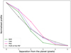 |
Fig. B.2 Corresponding mean azimuthal profiles for each correlation map above in Fig. B.1. |
| In the text | |
|
Fig. B.3 Simulations from the parametric study with the planet at 1750 K and the star at different separations. Correlation maps with CO in band 1A. |
| In the text | |
|
Fig. B.4 Simulations from the parametric study with the planet at 1750 K and the star at different separations. Correlation maps with H2O in band 1A. |
| In the text | |
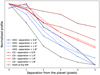 |
Fig. B.5 Corresponding radial profiles for each of the correlation maps of Fig. B.3 and Fig. B.4. |
| In the text | |
|
Fig. C.1 MIRISim simulation and correlation maps of the simulated system HR 8799. |
| In the text | |
|
Fig. C.2 MIRISim simulation and correlation maps of the simulated system ß Pictoris. |
| In the text | |
|
Fig. C.3 MIRISim simulation and correlation maps of the simulated system HD 95086 at 800 K. |
| In the text | |
|
Fig. C.4 MIRISim simulation and correlation maps of the simulated system HD 95086 at 1400 K. |
| In the text | |
|
Fig. C.5 MIRISim simulation and correlation maps of the simulated system HIP 65426. |
| In the text | |
|
Fig. C.6 MIRISim simulation and correlation maps of the simulated system 51 Eri. |
| In the text | |
|
Fig. C.7 MIRISim simulation and correlation maps of the simulated system HD 106906 the simulation plot shows the planet directly (in the center). |
| In the text | |
|
Fig. C.8 MIRISim simulation and correlation maps of the simulated system 2M 1207 at 1000 K. |
| In the text | |
|
Fig. C.9 MIRISim simulation and correlation maps of the simulated system 2M 1207 at 1600 K. |
| In the text | |
|
Fig. C.10 MIRISim simulation and correlation maps of the simulated system GJ 758. |
| In the text | |
|
Fig. C.11 MIRISim simulation and correlation maps of the simulated system GJ 504 for the three first channels. The scale is the same in each band and channel. |
| In the text | |
Current usage metrics show cumulative count of Article Views (full-text article views including HTML views, PDF and ePub downloads, according to the available data) and Abstracts Views on Vision4Press platform.
Data correspond to usage on the plateform after 2015. The current usage metrics is available 48-96 hours after online publication and is updated daily on week days.
Initial download of the metrics may take a while.