| Issue |
A&A
Volume 685, May 2024
|
|
|---|---|---|
| Article Number | A120 | |
| Number of page(s) | 20 | |
| Section | Planets and planetary systems | |
| DOI | https://doi.org/10.1051/0004-6361/202347068 | |
| Published online | 14 May 2024 | |
A new treatment of telluric and stellar features for medium-resolution spectroscopy and molecular mapping
Application to the abundance determination on β Pic b
1
LESIA, Observatoire de Paris, Université PSL, CNRS, Sorbonne Université,
Université Paris Cité, 5 place Jules Janssen,
92195
Meudon,
France
e-mail: flavien.kiefer@obspm.fr
2
Univ. Grenoble Alpes, CNRS, IPAG,
38000
Grenoble,
France
3
Laboratoire Lagrange, Université Côte d’Azur, CNRS,
Observatoire de la Côte d’Azur,
06304
Nice,
France
Received:
1
June
2023
Accepted:
11
February
2024
Molecular mapping is a supervised method exploiting the spectral diversity of integral field spectrographs to detect and characterise resolved exoplanets blurred into the stellar halo. We present an update to the method, aimed at removing the stellar halo and the nuisance of telluric features in the datacubes and accessing a continuum-subtracted spectra of the planets at R ~ 4000. We derived the planet atmosphere properties from a direct analysis of the planet telluric-corrected absorption spectrum. We applied our methods to the SINFONI observation of the planet β Pictoris b. We recovered the CO and H2O detections in the atmosphere of β Pic b by using molecular mapping. We further determined some basic properties of its atmosphere, with Teq=1748−4+3 K, sub-solar [Fe/H]=− 0.235−0.013+0.015 dex, and solar C/O=0.551 ±0.002. These results are in contrast to values measured for the same exoplanet with other infrared instruments. We confirmed a low projected equatorial velocity of 25−6+5 km s−1. We were also able to measure, for the first time and with a medium-resolution spectrograph, the radial velocity of β Pic b relative to the central star at MJD=56910.38 with a km s−1 precision of −11.3±1.1 km s−1. This result is compatible with the ephemerides, based on the current knowledge of the β Pic system.
Key words: techniques: imaging spectroscopy / planets and satellites: atmospheres / planets and satellites: composition / planets and satellites: formation / planets and satellites: gaseous planets / planets and satellites: individual: beta Pictoris b
© The Authors 2024
 Open Access article, published by EDP Sciences, under the terms of the Creative Commons Attribution License (https://creativecommons.org/licenses/by/4.0), which permits unrestricted use, distribution, and reproduction in any medium, provided the original work is properly cited.
This article is published in open access under the Subscribe to Open model. Subscribe to A&A to support open access publication.
1 Introduction
The system of β Pictoris, with its imaged debris disk of dust, evaporating exocomets and two giant planets, opens a stunning window into early stages of planetary systems formation and evolution. At the age of β Pic~23±3Myr (Mamajek & Bell 2014), giant planets have already formed, most of the protoplanetary gas has disappeared from the disk, and Earth-mass planets may be still forming. The discovery of β Pic b in direct high-contrast imaging (Lagrange et al. 2009) was rapidly recognised as a major finding for several reasons. First, until the discoveries of β Pic c (Lagrange et al. 2019; Nowak et al. 2020) and, more recently, AF Lep b (Mesa et al. 2023), it was the shortest period imaged exoplanet, thus enabling a ‘fast’ orbital characterisation. Second, once its mass is known, it can be used to calibrate brightness-mass models and atmosphere models at young ages. Third, it serves as a precious benchmark for detailed atmosphere and physical characterisations, thanks to its proximity to Earth and position with respect to the star. Finally, it is an exquisite laboratory for studying disk-planet interactions at a post-transition disk stage (Lagrange et al. 2010, 2012).
Model- and age-dependent brightness–mass relationships predict β Pic b mass to be within 9–13 MJ (Bonnefoy et al. 2013; Morzinski et al. 2015; Chilcote et al. 2017). Its mass is still marginally constrained observationally because of significant uncertainties on the amplitude of the radial velocities (RV) variations induced by the planets b and c. In particular, the available RV data do not cover the whole β Pic b period, the extrema of the recently discovered β Pic c-induced variations are not well constrained with the available data, while the RV variations are strongly dominated by the stellar pulsations (see examples in Lagrange et al. 2019, 2020; Vandal et al. 2020). Gaia data were used by several authors to further constrain the planet b mass: <20 MJ (Bonnefoy et al. 2013), 13±3 MJ (Dupuy et al. 2019), 12.7±2.2 MJ (GRAVITY Collaboration 2020), and 10–11 MJ (Lagrange et al. 2020). The most recent determinations combine RV, relative and absolute astrometry, taking into account both planets b and c. They lead to  MJ using the HIPPARCOS–Gaia DR2 measurement of astrometric acceleration (Brandt et al. 2021), and
  MJ using the HIPPARCOS–Gaia DR3 measurement of astrometric acceleration with the same datasets (Feng et al. 2022). We note that the astrometric acceleration measurement, also known as proper motion anomaly (see also Kervella et al. 2019, 2022), initially 2.54–σ significant using the DR2 (Kervella et al. 2019), became compatible with zero at 0.86–σ using the DR3 (Kervella et al. 2022). This explains the difference in the derived mass. From dynamical considerations, the mass of β Pic b is thus bounded within 9–15 MJ.
The study of infrared spectra emitted by transiting and non-transiting hot jupiter (Brogi et al. 2012, 2013, 2014; de Kok et al. 2013; Birkby et al. 2013, 2017; Lockwood et al. 2014; Piskorz et al. 2016, 2017; Guilluy et al. 2019; Cont et al. 2021, 2022a,b; Yan et al. 2022) and young imaged planets (Snellen et al. 2014; Brogi et al. 2018; Hoeijmakers et al. 2018; Petit dit de la Roche et al. 2018; Ruffio et al. 2019, 2021; GRAVITY Collaboration 2020; Cugno et al. 2021; Petrus et al. 2021; Patapis et al. 2022; Petrus et al. 2023; Mâlin et al. 2023; Miles et al. 2023; Landman et al. 2023) allows us to characterise the atmospheric composition in molecules such as CO, CO2, H2O, NH3, and CH4. The molecular mapping method was first developed for this objective by Snellen et al. (2014), hereafter S14, for medium-or high-resolution instruments such as CRIRES (S14, Landman et al. 2023), SINFONI (Hoeijmakers et al. 2018; Cugno et al. 2021; Petrus et al. 2021), Keck/OSIRIS (Petit dit de la Roche et al. 2018; Ruffio et al. 2019, 2021), or JWST/MRS (Patapis et al. 2022; Mâlin et al. 2023; Miles et al. 2023). This method consists in calculating the cross-correlation function (CCF) of a spectrum emitted from the atmosphere of a planet with a theoretical transmission spectrum, or template, using for instance Exo-REM (Baudino et al. 2015; Charnay et al. 2018). This could reveal the presence of individual molecules. The CCF leads to a similarity score, which if equal to 1 (0) means the spectrum and the template are proportional (totally orthogonal). In general, because of noise, systematics, and inaccuracies of models, a CCF never reaches exactly 1. Using the CCF as a template matching score in principle allows us to retrieve simple atmospheric properties such as Teff, log 𝑔, and relative abundances.
For β Pic b, Hoeijmakers et al. (2018, H18 hereafter) showed using molecular mapping on the cubes collected by the Spectrograph for INtegral Field Observations in the Near Infrared (or SINFONI) that H2O and CO were present in the atmosphere of this young planet, with no evidence of other species. They did a tentative template matching of Teff and log 𝑔 that led only to large confidence regions of those parameters on their Fig. 10. They did not produce any estimation of the planet radial velocity, nor the rotational broadening, υ sin i.
With a spectrum-fitting oriented approach, an emitted spectrum of β Pic b was obtained with GRAVITY (GRAVITY Collaboration 2020). Its fit led, in a Bayesian inference framework using Markov chain Monte Carlo sampling of posteriors, to an effective temperature of 1740± 10 K with log 𝑔=4.35±0.09, a super-solar metallicity of [M/H]~0.7±0.1 and a sub-solar of C/O=0.43±0.041. This was in good agreement with previous estimations of the planet temperature of 1724K and a log 𝑔 = 4.2 by Chilcote et al. (2017) and the combined astrometric+RV planet mass estimation ~12 MJ (Snellen & Brown 2018; GRAVITY Collaboration 2020; Lagrange et al. 2020). However, the metallicity was significantly different if considering the GRAVITY spectrum only (−0.5 dex) or combined with the GPI YJH low-resolution spectra (>0.5 dex). Most recently, Landman et al. (2023) published the analysis of new β Pic b high-resolution spectra taken with the upgraded CRIRES+ instrument that led to similar parameters using atmospheric retrievals, with temperatures slightly higher than in GRAVITY Collaboration (2020), a sub-solar metallicity (Fe/H~−0.4) and a sub-solar C/O=0.41±0.04. Thanks to the high resolution of the instrument, they were able to obtain a new υ sin i measurement of 19.9±1.1 km s−1.
Using an approach similar to that of GRAVITY Collaboration (2020), Petrus et al. (2021) used both a principal component analysis (PCA) and halo-subtraction on north-aligned angular differential imaging (nADI) on SINFONI observations of HIP 65426 to extract the emitted spectrum of the planet b keeping the thermal continuum. They then used Bayesian inference with nested sampling (Skilling 2006) to retrieve the basic parameters of planet HIP 65426 b from the spectrum itself, including equilibrium temperature, surface gravity, metallicity ratio [M/H], and C/O. This demonstrated that it was possible to derive the spectrum of a planet observed with SINFONI and that having a spectrum-fitting, rather than CCF-optimisation method, leads to more reliable results.
In this work, we performed a new analysis of the β Pic cubes observed with SINFONI. We improved the reduction of the cubes, as explained in Sect. 2. We then improved the star removal method used by H18 with a different approach, which corrects for residuals from the stellar lines. We discuss the H18 method and explain our improvements in the form of a new method called starem in Sect. 3.2. Then, in Sect. 4, we apply a molecular mapping and compare it to the H18 results. We further extract the spectrum of the planet in Sect. 5. We use a simple grid search as well as a Bayesian framework with an MCMC sampling to fit the observed planet spectrum and measure the parameters of the planet. This is done in Sect. 6. We discuss the results in Sect. 7 and give our conclusions in Sect. 8.
2 SINFONI data pre-processing
2.1 SINFONI observations
SINFONI was an infrared instrument, coupling an adaptive optics (AO) module to an integral field spectrograph (IFS) SPIFFI, installed on the Unit Telescope 4 of the Very Large Telescope at Paranal/Chile (Eisenhauer et al. 2003; Bonnet et al. 2004). SINFONI was on-sky from 2004 to 2019. Observations with the SINFONI IFS were performed with different sizes for the field-of-view (FoV) and spectral resolution (R), then reduced into data cubes, with two spatial and one spectral dimensions. Here, we focus on observations of the β Pictoris surroundings performed with the 0.8″×0.8″ FoV subdivided into 64×64 spaxels2 of size 12.5×12.5-mas2 at R=4000 along the K-band (2.08−2.45 µm). The observations consist in 24 exposures of 60 s each, recorded on the 10th September 2014 from 08:19:34 UT to 10:05:20 UT. An offset of 0.9–1.1″ from β Pic and a field rotation of −56° to −19° was applied, reducing the pollution of the stellar halo upon the planet spaxels with the star decentred outside the FoV, focusing the observations on the surroundings of β Pictoris, and enabling the use of angular differential imaging (Marois et al. 2006). The seeing during the observation varied within 0.8–1.0″ with an airmass varying from 1.35 to 1.14 between the first and the last exposure. The atmospheric conditions were relatively constant during the observations, with fluctuations of pressure and temperature of <1%.
2.2 From SINFONI raw data to registered cubes
We performed the data reduction of the SINFONI sequence of observations following the scheme described in Petrus et al. (2021), which provides optimally-reduced datacubes for high-contrast science.
The raw data were originally corrected the Toolkit for Exoplanet deTection and chaRacterisation with IfS (hereafter, TExTRIS; Petrus et al. 2021; Palma-Bifani et al. 2023; Demars et al. 2023, Bonnefoy et al., in prep.) from the so-called ‘odd-even’ effect affecting randomly some pre-amplification channels on SPIFFI’s detector (corresponding roughly to the location of the 25th slitlet). We then used the ESO data handling pipeline version 3.0.0 to reconstruct data cubes from the bi-dimensional science frames. TExTRIS also corrected for the improper registration of the slitlet edges on the detector and for the inaccurate wavelength solution found by the pipeline using synthetic spectra of the telluric absorptions.
Finally, we used TExTRIS to perform a proper registration of the star position outside the field of view. H18 fitted a synthetic function to represent the wings of the star’s point spread function (PSF). However, such a method is sensitive to the distribution of flux within the FoV. The later can be affected by (i) the complex evolution of the Strehl ratio that evolved with wavelength and along the sequence, cubes with high Strehl ratios, showing strong artefacts due to the telescope spiders (while those with low Strehl ratio show a smoother flux distribution) and (ii) the varying part of the halo contained in the FoV due to the field rotation along the sequence. TExTRIS uses instead an initial measurement of the star position in data cubes acquired during short exposures taken at the beginning of the sequence and centred on the star. Then it builds a model of the β Pic centroid positions, which are located outside the FoV in the 24 exposures of the observation sequence, by computing their theoretical wavelength-dependent evolution due to the evolving refraction, the field rotation, and the offsets on sky.
A remaining error due to telescope flexure exists (see the ESO user manual) but appears to be below ~1 pixel in the final registered cubes of β Pictoris. This reduction provides us with 24 data cubes and associated measurements of the offsets and rotation angles that will be used in Sect. 2.5 to de-rotate and stack the cubes aligned on the position of the planet β Pic b.
2.3 Reference stellar spectrum
First, we define the method we used throughout this study to derive a reference stellar spectrum, free from photons coming from the planet, in the K-band using a SINFONI data cube. We found it best to use several of the brightest spaxels within a cube and combine them to obtain a stellar spectrum to reduce any pollution from the background and the planet. To find those, for all spaxels of the FoV, we measured the flux at the continuum-level of the Br-γ line at ~2.165 µm by fitting the wings of the line by a two-degree polynomial and retrieving the level of the continuum at 2.165 µm. From this flux map, we excluded the 10 brightest spaxels to avoid bad spaxels and calculated an average star spectrum from the next 100 brightest ones. Those are the less affected by the background whose level is on the order of −20 erg s−1 cm−2 Å−1 while the total flux reaches more than 2000 erg s−1 cm−2 Å−1. Therefore, its contribution is less than 1% in those spaxels. Figure 1 shows the absolute total and residual flux distribution among spaxels of the stacked cube obtained in Sect. 2.5 below. The resulting reference star spectrum is showed on Fig. 2. We note that it includes many telluric lines beyond 2.18 µm, mainly H2O, CO2, and CH4 lines.
2.4 Wavelength calibration correction
The presence of telluric lines is a nuisance to the analysis of stellar and exoplanet spectra. Nonetheless, they can also be used to adjust the wavelength calibration in the SINFONI cubes. Tellurics can be fitted directly in each of the 24 cubes to the normalised star spectrum. Since we are most interested in the planet, the star spectrum is here obtained from the spaxels located at the position of the planet. The planet position in the derotated cube is determined in Sect. 4.2 and its PSF of the four-spaxel FWHM in Sect. 3.2. We calculated for each cube the mean stellar spectrum on a circular area of six–spaxel radius around the planet location.
We used the ESO code molecfit (Smette et al. 2015; Kausch et al. 2015) v3.13.6 that implements LBLRTM to perform the telluric line fit in this spectrum. Typical site parameters during the observations are taken as inputs, such as the MJD, paranal altitude and coordinates, humidity (~4%), ambiant pressure (~740 hPa), ambiant temperature (~12°C), mirror temperature (~10.9°C), and airmass (sec z~1.1–1.4). molecfit fits the atmospheric parameters (such as water column abundance, pressure, temperature, and so on) as well as a continuum, a Chebychev polynomial wavelength solution, and a line spread function to the observed telluric lines in the observed spectrum. The error bars are fixed to the square root of the flux divided by the normalisation. The observed reduced χ2 are consistent within 1.3–1.4 all through the cubes time series. We found that the molecules H2O, CO2, CH4, and N2O dominate the model tel-lurics spectrum in the K-band, whilst CO, NH3, O2, and O3 are always either weak and undetermined or fitted to negligible relative abundance values <10−4. To reduce the computation effort, we thus only fit for H2O, CO2, CH4, and N2O column densities. A polynomial of a degree of 6 for the fit of the continuum and of degree of 1 for the fit of the wavelength solution was adopted. We fixed the LSF to a Gaussian function, allowing its width to vary. The LSF is moreover convolved in molecfit by a 1-pixel (0.00025 µm) box to mimic the effect of the slit smearing.
Figure 3 shows a summary of the molecfit solutions along the cubes. Figure 4 shows the β Pic stellar spectrum compared with the molecfit resulting model. There is a residual time-dependent shift of the wavelength solution even after the absolute calibration performed by TexTRIS of about 8 km s−1 from first (cube 0) to last (cube 23) exposure. This agrees with the magnitude of the error on the calibration found in Petrus et al. (2021). Such shift could be due to an effect of flexure of the instrument. We corrected the wavelength solution in all cubes according to this analysis. The figure also shows that the resolving power is varying through the observation series with an LSF FWHM of ~2.16–2.32 pixels at 2.27 µm. This variation is due to the wandering of the planet image on the detector. This leads to an average effective resolving power in our SINFONI K-band spectra of R=4120±90.
The atmospheric molecular column density of H2O is relatively constant along the observation sequence. We note that the CO2 abundance level of ∼500 ppmv retrieved is ~1.4 times higher than the reference value (∼370 ppmv) in the model Earth atmosphere, while N2O abundance ∼0.30 ppmv is about 1.2 its reference level. At the same date and using the whole K-band spectrum (including deep CO2 and N2O lines below 2.07µm) of another reference star, the CO2, and N2O abundances reach ∼390 ppmv and 0.23 ppmv, respectively (Smette, priv. comm.). Relying on weak lines only, our determination of the CO2 and N2O abundance levels might not be well determined. The absolute values of the species abundances presented here should thus be considered as indicative only.
Applying the same procedure on the star spectrum taken from other locations in the image led to similar molecular abundances. However, it revealed a strongly scattered resolving power within 3500–4900, though the average value of R agreed on an effective resolving power of ∼4000. This is much smaller than the theoretical R=5950, expected for SINFONI in this setup. This might be explained by the degradation due to pixelation when creating the cubes, since the LSF sampling is sub-Nyquist, with a spectral broadening of about 1.5 pixels as noted in the latest SINFONI’s documentation3.
A thorough investigation on how to improve the effective spectral resolution in the reduced data of instruments such as SINFONI is not in the scope of the present study. Nevertheless, with regard to such objective, two leads might be worth mentioning: (i) achieving a finer reconstruction of cubes from the 2D images of the slitlets and the arc lamp calibration, or more simply, yet at the expense of time, or (ii) using dithering during the observations to better sample the LSF, at the cost of at least doubling the exposure time. These leads will be explored in further studies.
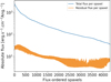 |
Fig. 1 Absolute total (blue) and residual (orange) flux per spaxel. The spaxels are ordered from the brightest to the faintest in absolute total flux per spaxel. The absolute total flux is the raw flux obtained as output of the stack phase in Sect. 2.5. The residual flux is the remaining absolute flux once the star spectrum is removed (see Sect. 3.2 for more details). |
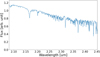 |
Fig. 2 Star spectrum calculated from the brightest spaxels. The flux is normalised to the pseudo-continuum flux at the top of the Br-γ line at 2.165 µm. |
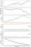 |
Fig. 3 Summary of molecfit results. First panel: wavelength solutions showing the Doppler shift against the wavelength through the K-band with respect to cubes series number. Second panel: measured resolving power from FWHM of the fitted LSF. Third and fourth panels: fitted ppmv abundances of H2O, CO2, CH4, and N2O. |
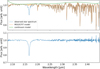 |
Fig. 4 Stellar spectrum observed with SINFONI (blue) compared to the model Earth telluric spectrum calculated with molecfit (orange) and the continuum model (green). Upper panel: two spectra compared directly. Lower panel: stellar spectrum divided by the telluric spectrum model. |
 |
Fig. 5 Steps of star spectrum removal methods compared. Qobs stands for the stacked cube observed, while |

2.5 Science cubes stacking
We aligned the 24 science cubes taken on the 17th of November upon the star centroid. Then, the cubes were de-rotated in such a way that the planet halo is brought at the same (α*,δ)-coordinates in every cube and at every wavelength. We use the values obtained with TExTRIS as explained in Sect. 2.2. This includes a 2D linear interpolation using the interpolate.griddata routine from scipy in order for all the shifted-rotated cubes to share a common (α*,δ)-grid. Then the 24 cubes are stacked together using a simple average. No clipping of flux is applied during this process in order to maximise the signal-to-noise ratio (S/N). This gives us the data cube that we use in the rest of the analysis; we name it the ‘master cube’ and it is denoted Qobs.
3 Star spectrum removal with STAREM
3.1 A summary of H18 method
The H18 method used to remove the stellar halo proved to work well for performing molecular mapping of exoplanets. However, it does not allow for the extraction of a pure planet atmosphere transmission spectrum where systematic deviations remain. We will summarise the H18 method here to show where is the identified issue. A sketch of the different steps of this method is shown in Fig. 5. The components of the flux at the planet spaxels, ip, are as follows:
 (1)
(1)
Among these parameters, the star flux,  and the planet flux,
  , as well as a possible background component,
  (setting the latter aside at present for the simplicity, we note that it can be added everywhere by duplicating the planet components and changing ‘p’ with ‘B’ in the index; see discussion in Sect. 3.3). We also dropped the ‘ip’ index in the following to alleviate the equations.
The planet and star spectra are each composed of a continuum (hereafter denoted C) multiplied by a ‘flat’ transmission spectrum, whose continuum is normalised to 1 everywhere (hereafter denoted η). Both the astrophysical source and telluric lines contribute to this transmission spectrum. This can also be expressed as η=1 − A, with A as a positive comb of spectral lines with the continuum equal to zero everywhere. We point out that the A⋆ and Ap values for the star and the planet, respectively, are supposed to be spaxel-independent, since they are intrinsic to the respective sources. The continua Cp and C⋆ are on the other hand spaxel-dependent because of the PSF and the wavelength-dependent speckles.
In H18, to remove the star and single-out the planet, an approximated star spectrum Fi,⋆,approx that accounts for wavelength-dependent spaxel-to-spaxel variations was subtracted from each spaxel, i, of the cube, Qobs. They divided each spaxel spectrum by the star spectrum determined (as explained in Sect. 2.3) by averaging some of the brightest spaxels of the master cube. The ‘star-free’ cube Qstar-free thus obtained displays low-frequency wavelength-dependent variations that differ in the spectra from one spaxel to the other. They are due to speckle patterns over the detector changing with wavelength. Those speckle patterns are modeled by applying a Gaussian filter, G, on this star-free spectrum, G * Qstar-free. It results in a speckle-proxy cube, denoted Qspkl in Fig. 5. By multiplying those modelled variations by the star spectrum, they finally obtained the star cube Q⋆, with a star spectrum, Fi,⋆,approx, at each spaxel, i, which accounts for wavelength-dependent spaxel-to-spaxel variations.
At any spaxel other than the planet spaxels, subtracting Fi,⋆,approx removes the contribution of the star spectrum. However, at the planet spaxel, this is not valid. Indeed, the approximated star spectrum contains contributions from both the star and the planet continuum:
 (2)
(2)
By slightly overestimating the star contribution, the subtraction of F⋆,approx instead leads to:
 (3)
(3)
A supplementary stellar contribution (including tellurics) to the residual absorption spectrum remains seen as emission lines, with amplitudes comparable to the planet absorption lines. This is shown in Fig. 6. We note that the persistence of polluting CH4 lines led H18 to apply several runs of SYSREM (Tamuz et al. 2005) to remove them. However, this operation does not fix the above issue and the stellar lines still remain in the spectrum at the planet spaxels.
The presence of the star spectrum with a non-negligible amplitude is problematic. Moreover, since the continuum has been subtracted, there is no longer any reference level to which we can compare the strength of molecular lines in the resulting spectrum. As long as the CCF of the star spectrum and the spectra of any of the species found in exoplanet atmosphere is close to zero, this works well for molecular mapping. This is the case here with a 8000 K star and a <2000 K planet. Nonetheless, ∆F is not strictly-speaking a pure planet atmosphere spectrum. This issue might also explain the detection of an Br-γ emission line in the PDS-70b spectrum derived with the same H18 method in Cugno et al. (2021). Thus, we suspect it is an artefact from the stellar spectrum removal.
 |
Fig. 6 Raw β Pic b spectrum extracted from the planet spaxels after using H18 method of star light removal. SYSREM was not used here. We highlight in red the main artefact that is due to excess star spectrum lines removal at the Brackett-γ wavelength. We also note that since the continuum has been subtracted, the reference level to which compare the strength of planet molecular lines (CO shown in green) is missing. |
3.2 STAREM: A new STAr spectrum REMoval method
We propose a different method to subtract the star spectrum, which we named STAREM and which instead makes use of the normalised transmission spectrum, η=F/C. In this spectrum, we aim to estimate the contribution of the star in any spaxel spectrum, Fi, by fitting the stellar absorption lines and then subtracted it from Fi. We demonstrate that this can lead to a well defined flattened transmission spectrum of the planet atmosphere, where the star spectrum is fully removed and the line strength is preserved.
First of all, we normalise all spectra of the observed cube, as well as the star spectrum, by fitting a sixth-degree polynomial to their continuum, leading to a normalised star spectrum of F⋆,norm and a normalised cube of Qobs,norm. Recalling Eq. (1), the normalised transmission spectrum components of F = C η at one of the planet spaxels in Qobs are:
 (4)
(4)
We recall that the star and planet pseudo-continua are fixed by the star and planet intrinsic pseudo-continua multiplied by the Strehl ratio and PSF (including speckles) damping of the flux. We introduce the star and planet contribution levels, K⋆ and Kp, as:
 (5)
(5)
The transmission spectrum η(λ) can be expressed more compactly as:
 (6)
(6)
If we wish to subtract the star contribution, K⋆ η⋆, from this spectrum, we need to estimate K⋆(λ). This can be achieved by comparing the amplitude of the stellar lines to those of a reference stellar spectrum without contributions from the planet; here, a ratio of 1 implies a pure stellar spectrum, namely, K⋆=1. Ideally, with several stellar lines present all through the observed band, the best approach would be to use all the lines so as to obtain a more reliable wavelength-dependent approximation of the K⋆(λ) function. In the specific case of the K-band spectrum of β Pic, since the Brackett-γ line at 2.165 µm is the only strong feature in this spectral band, we were only able to derive an approximated constant star contribution ~K⋆(λ0=2.165 µm); also noted as K⋆,2.165 hereafter. The derived values of K⋆,2.165 and its pendent residual contribution, 1 −K⋆, through the SINFONI field-of-view around β Pic b, are shown in Fig. 7.
Removing an approximated contribution, K⋆,2.165 η⋆, at each spaxel of Qobs,norm leads to a residual cube Qres. In this cube, the residual spectrum obtained on a planet spaxel is:
 (7)
(7)
Using Eq. (5), this could equivalently be written as:
 (8)
(8)
This is a flat spectrum whose baseline level is Kp,2.165= 1−K⋆,2.165. At the planet spaxels, it should contain the normalised spectrum of the planet with an amplitude corresponding to the relative flux of the planet compared to the star at 2.165 µm. Because of the normalisation of the planet spectra by the continuum of the star, this is only an approximation. Indeed, away from Brackett-γ (more generally from any fitted stellar line) the line amplitudes are impacted by a residual star spectrum component with an amplitude of δK(λ)=Kp,2.165 −Kp(λ). This is a footprint of the planet and the star continua within the flat spectrum. Unfortunately, we cannot assume that δKη⋆≈0 because it generates a warp of the planet spectrum lines deviating from one to a few tens of percent, as shown in Fig. 8. This will have to be taken into account later on when analysing the spectrum extracted from the planet spaxels.
 |
Fig. 7 Star flux fraction, |


 |
Fig. 8 Warp function δK(λ) (orange) normalised to 1 at the Brackett-γ wavelength (top panel), compared to a normalised Exo-REM model with T=1750K, logg = 4.0, [Fe/H]=0.0, and C/O=0.55 (blue) as well as the normalised stellar spectrum |

3.3 Tellurics and background removal
In Sect. 2.4, we describe how the tellurics were fitted directly in each of the 24 cubes to the normalised reference star spectrum obtained from the brightest spaxels. They were only used for purpose of calibration. We did not wish to remove tellurics at the next step because removal might introduce residuals with amplitudes on the order of magnitude – or worse, even larger amplitudes than the planet would feature.
With the residual cube, Qres, in hand, which mainly features the planet and background, we now wish to remove the many tellurics lines that are still present in the observed spectrum in the K-band. In a more straightforward way, we could fit a model telluric spectrum to any spaxel spectrum in the cube using molecfit. However, it is quite time consuming to run molecfit with a cube of about 10 000 spaxels and also given the S/N of the residual spectra is poor. Instead, we preferred to use molecfit on the star spectrum derived from the stacked cube at the position of the planet. This allows us to obtain a reliable telluric model, ηmodel, to correct again the wavelength solution, using the same settings as in Sect. 2.4. In doing so, we determined the effective spectral resolution at the position of the planet in the stacked cube to be 4020±30.
At each spaxel, i, of the residual cube, we fit out this telluric model, ηmodel, from ηi,res. To do so, we first needed to correct for a wavelength-dependent background contribution whose nonzero level causes an artificial decrease in the prominence of the telluric lines and the appearance of spurious features, such as telluric lines residuals. These can be seen by comparing a planet-spaxel spectrum and its surrounding background (Fig. 9). The origin of the continuum level of the background is unknown, but it could be due to scattered stray light. The features are generated by the differences between the stellar (plus telluric) spectrum actually observed at the given spaxel and the reference stellar (plus telluric) spectrum (removed in Sect. 2.34).
We make an estimation of the background contribution in a spaxel i by taking the median spectrum in a distant ring around this spaxel ηi,ring. Since the SINFONI PSF has a FWHM of ~4 spaxels in radius, we used a ring radius of six spaxels with a width of one spaxel. This background estimate is then removed from the spaxel, i, spectrum of ηi,res,corr = ηi,res − ηi,ring. Its contribution level at ~2.165 µm can be viewed (in Fig. 7) in the brighter areas away from the planet’s location. Figure 1 also shows the 2.165-µm absolute background flux, which is ~1–10% of the absolute total flux at every spaxel. Around the planet location, its continuum level is very close to zero, but non-negligible features are seen that have corresponding features in the spectrum at the planet’s central spaxel.
Adding a background term to Eq. (8), the background subtraction can be summarised with the following set of equations:
 (9)
(9)
Assuming an equal contribution ofbackground in the central and the neighboring spaxels, namely, Ki,b = Kring,b, this equation can be simplified to:
 (10)
(10)
Thus, we are able to recover Eq. (8) and the previously implicit background is now explicitly suppressed. The final step is to fit ηmodel (the telluric spectrum model) to ηi,res,corr· We use a simple least-squares optimisation at each spaxel, allowing the telluric model to vary in intensity with ηi,tell = a ηmodel + b with a + b = ci, if ci is the level of the residuals at spaxel i. Because ηmodel was determined from the reference stellar spectrum (which could be a slightly affected by the background), an offset (b) is added to account for small intensity differences in telluric lines between ηmodel and the telluric spectrum at a spaxel, ¡. We divide ηi;tell from ηi,res,corr, leading to the telluric-free spectrum of ηi,res,tell-free. A summary of the background subtraction and telluric removal at the central planet spaxel is shown in Fig. 9.
 |
Fig. 9 Background-subtraction and telluric removal from a planet-spaxel spectrum. Top: planet spaxel spectrum and average background on a distant ring. Middle: ηres,corr compared to its fitted telluric model ηtell. Bottom: planet-spaxel spectrum corrected from background and tellurics. |
4 Molecular mapping dedicated to SINFONI spectra
4.1 Exo-REM grid of models
To determine the molecular mapping of diverse species in the atmosphere of β Pic b, as is now most commonly performed (see e.g. Snellen et al. 2014; Brogi et al. 2018; Hoeijmakers et al. 2018; Petit dit de la Roche et al. 2018; Ruffio et al. 2019; Cugno et al. 2021; Petrus et al. 2021; Patapis et al. 2022; Mâlin et al. 2023), we calculated a CCF of the observed spectrum at each spaxel with a synthetic spectrum. Here, the templates are taken from an Exo-REM model grid (Baudino et al. 2015; Charnay et al. 2018; Blain et al. 2021). Exo-REM is a 1D radiative-convective model, which self-consistently computes the thermal structure, the atmospheric composition, the cloud distribution and spectra. The model includes the opacities of H2O, CH4, CO, CO2, NH3, PH3, TiO, VO, FeH, K, and Na, along with the collision-induced absorptions of H2–H2 and H2–He. Silicate and iron clouds are included using simple microphysics to determine particle sizes (Charnay et al. 2018). The model grid includes four free parameters totaling 9573 spectra, with Teq ranging from 400 to 2000 K with steps of 50 K; log g from 3.0 to 5.0 dex with steps of 0.5 dex; and [M/H] from −0.5 to 1.0 dex with steps of 0.5 and [C/O] from 0.1 to 0.8 with steps of 0.05. The synthetic spectra were computed at R=20 000, which reflects a compromise between reducing computation speed and reaching the highest resolution possible on atmospheric models to be used as templates of low-to-medium resolution spectra of exoplanets.
We cleansed the model grid from those that did not converge well. To do so, for each spectrum, we calculated the integral on the whole wavelength domain from visible to far IR, Is. We compared this integral to the theoretical  Stefan-Boltzman law.
This deviation peaks below ~5% (Fig. 10). We thus removed 3315 among 9573 spectra (i.e. 35%) with a deviation larger than 5%.
Each synthetic spectrum produced by Exo-REM results from individual contributions (or spectrum) of the species out of which it is composed, mainly CO, H2O, CH4, and NH3, which we can use as individual molecular templates.
 |
Fig. 10 Histogram of relative difference between the exo-REM models emittance and Stefan-Boltzman law. |
4.2 The cross-correlation function of the planet spectrum
At every spaxel, between 2.08 and 2.43 µm, we calculate the CCF of the observed spectrum and an Exo-REM synthetic spectrum for an assumed Teff=1700 K, log g=4.0 cgs, and [Fe/H]=0.0 dex, as based on Table 3 in GRAVITY Collaboration (2020). The expected abundances of NH3 and CH4 in the atmosphere ~10−6 are too low to yield absorption features detectable in the SINFONI spectra. Thus, we artificially enhanced their abundances to 10−4, in order to probe possible over-abundance of these species in β Pic b’s atmosphere. Details on the contributions of H2O, CO, NH3 and CH4 are shown in Fig. 11 and compared to the β Pic b’s spectrum derived in next Sect. 5.
We excluded the red edge of the K-band beyond 2.43 µm, which displays the strongest telluric lines remnants. Prior to the calculation, we divided the continuum of the observed and synthetic spectra. The continuum is obtained by first fitting a fourth-degree polynomial and then applying a median filter with a window-width of 0.01 Å, combined to a smoothing Savitzky-Golay filter of order 1. The CCF is calculated by directly cross-correlating the median-removed observed and synthetic spectra at different shifts. The CCF is finally normalised by the norm of the spectra, thus leading to a zero-normalised CCF. This results in the molecular maps shown in Fig. 12.
We then fit the PSF of the planet CCF halo by a 3D Gaussian with respect to (δ, α, vr). This determines the position and radial velocity of the planet, as well as the broadening of the PSF and of the LSF. The results are summarised in Table 1. They are compared to the values derived in the same fashion but following H18’s recipe to suppress the stellar pollution. We only show the results for CO, H2O, and (using the full spectrum, confirming, as in H18) the presence of CO and H2O, but not detecting NH3 and CH4. With some variability from one model to the other, the CCF peak is located at a separation to the central star of ~351 ± 5 mas, with a PSF broadening standard deviation of ~2.7 spaxels, that is 34 mas.
The S/N is calculated as the height of the peak divided by the fit residuals on a volume of 200 pix2 by 2000 km s−1 around the planet (δ,α,vr)-location. Our starem method leads to S/N values that are comparable to those obtained through H18 method. We did not use SYSREM as they did to remove the spaxel-to-spaxel correlated noise within the cubes, but corrected for the background differently (as explained in Sect. 3.3). We derived a slightly better S/N by subtracting the star halo using STAREM (instead of those obtained using the H18 subtraction method), leading to S/Nall=19.6, S/NCO=11.8, and  . This also follows the trend found for HIP 65426 b (Petrus et al. 2021), whereby taking into account all species leads to the best detection S/N; while for individual contributions of species, H2O gives significantly better results than CO. These last properties is best explained by the presence of less prominent but more numerous lines of H2O compared to CO all along the K-band and, especially, away from regions spanned by telluric lines.
We note that in H18 paper, the S/N values they obtained are greater (all molecules: 22.8 vs. 17.5 here; CO: 13.7 vs. 11.2 here; H2O: 16.4 vs. 15.7 here). This difference can be explained by the fact that they averaged the CCF of cubes obtained at two different nights, while we used the cubes from only a single night. The smaller difference of S/N for H2O can be explained by the presence of traces of telluric lines in the H18 residual cube because they did not recalibrate the wavelength solution before subtracting the reference spectrum (containing the tellurics). We also note that the calculation performed in H18’s paper to determine the S/N is slightly different in that they use a distant 3D-ring around the CCF peak to estimate the noise, while we calculate the noise from the residuals of a fit of the CCF peak.
 |
Fig. 11 SINFONI planet absorption spectrum of β Pic b along the K-band, once corrected from star, background, and telluric pollutions (top). Exo-REM spectrum of simulated atmosphere of 1700 K, log(g)=4.0, and [Fe/H]=0.0 with R=6000 (bottom). Individual contributions of species CO, H2O, CH4, and NH3 are represented from top to bottom with diverse colors. For all the spectra, their continuum were divided, as explained in Sect. 4.2. |
 |
Fig. 12 Molecular CCF maps of β Pic b for species CO, H2O, CH4 (10−4) and NH3 (10−4). At each spaxel, the maps show the CCF height at 0 km s−1, a value close to the expected radial velocity of the planet b, |VR|<10 km s−1 given the instrument LSF of ~75 km s−1. |
Comparing results of the different star spectrum subtraction schemes on the normalised CCF of the residual map with a 1700 K, log g=4.0, [Fe/H]=0.0 Exo-REM model, detailing the CO and H2O individual contributions.
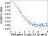 |
Fig. 13 Planet PSF radial profile at a varying distance from 0 to 8 spax-els. The relative flux is obtained by dividing out the continuum and subtracting the star spectrum, as explained in Sect. 3.2. |
5 Extracting the planet atmosphere absorption spectrum
The PSF of the planet follows an Airy profile whose central region can be approximated by a Gaussian profile. This can be seen in Fig. 13 where the residual flux of the stellar subtraction at 2.165 µm is shown with respect to the distance of the spaxels to the planet centre position. The planet centre position is obtained by fitting the residual flux at 2.165 µm by a 2D Gaussian. The radial profile of the planet PSF is well modeled by a two-spaxel wide Gaussian. The planet relative flux rises up to 7% near the centre, but becomes negligible compared to noise beyond a distance of about five spaxels.
The average spectrum at those spaxels is calculated by integrating the relative flux on all spaxels up to a given radius and applying to each spaxel a weight that depends on its distance to the planet. We model the PSF profile by the Gaussian used above, with  and where r=||r i− rc|| is the spaxel-distance between a given spaxel, i, and the planet centre position, and σPSF=2 spaxels at 2.165 µm. We used this profile as the weight function with thus
  . When integrating the spaxels flux, both planet and noise signals grow, yet they are still limited by the PSF flux dimming, and the S/N increases as
  · We found it reasonable to integrate the flux up to 4–σ from the PSF centroid, with σ(λ)=σpsF × 2.165 µm/λ.
Since we cannot assume that the background removal was absolutely perfect in Sect. 3.3, we again estimate the background pollution within planet spaxels using neighboring spaxels in a ring around the planet. The background level at distance to the planet centroid is close to zero within ± 0.01, as can be seen in the PSF profile (Fig. 13). We use the median spectrum within this ring as an estimation of the background spectrum shown in the top panel of Fig. 14. This background spectrum is subtracted from the average planet spectrum, leading to the corrected planetary spectrum, also shown Fig. 14. We found the ring radii optimising theS/N of the corrected planet spectrum to be4.2–5.1 spaxels.
As a final step, the spectrum was divided by the continuum and estimated (as in Sect. 4.2) by applying a median filter with a window-width of 0.01 Å combined to a smoothing Savitzky-Golay filter of the order of 1. The final planet spectrum obtained is compared to a theoretical Exo-REM spectrum of a 1700 K planet, with log g=4.0 cgs and [Fe/H]=0.0 dex in Fig. 11.
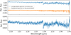 |
Fig. 14 Background removal. Top panel: average spectrum about the planet centroid (blue) compared to the average background spectrum on a ring around the planet (orange). Common features can be well distinguished. Bottom panel: planet spectrum corrected from the background. The features remaining are β Picb’s atmosphere absorption lines, while the main stellar feature (Brackett-γ) has been fully removed. |
6 Template-matching of the planet spectrum
We addressed the problem of finding the best matching model of the planet spectrum in two ways: first, by exploring the space of available templates and their match with the planet spectrum, using a simple grid search, and, second by running a Markov chain Monte Carlo (MCMC) sampling around the optimum spectrum. In both cases, we used the forward-modeled Exo-REM (Charnay et al. 2018) spectra models of exoplanet atmosphere.
6.1 Grid search
We first explored the template space by a grid search. We tested the χ2 and zero-normalised CCF scores for optimising the models. Each model spectrum is convolved by a Gaussian Kernel corresponding to a resolving power of 4020 and by a rotational profile with v sin i=25 km s−1. The rotational profile is the usual bell-like profile with limb-darkening coefficient ε=0.6 (Gray 1997). Each model spectrum is then flattened with the same median filtering function, with a window width of 0.01 µm, as used to flatten the observed spectrum. Moreover, we corrected for the 'warp' effect (noted in Sect. 3.2) in the models by adding a supplementary term in (1 − Cp/C) η⋆, with η⋆ as the normalised star spectrum, Cp as the model’s continuum, and C as the average continuum in the SINFONI cube at the planet spaxels, both normalised to 1 at 2.165 µm. For the ZNCCF, the median of both the model and data results is subtracted before the cross-correlation is done. For χ2, the fit function includes two other parameters applied to the model spectrum of a scale, a, to allow us to compensate for the arbitrary level of the spectrum continuum, and a rigid Doppler shift, vr. The fit is then performed using the curve_fit procedure from the scipy library.
The error bars of data points are derived from the relation of  , with F⋆,approx(λ) the reference stellar spectrum defined in Sect. 2.3 and C(À) the continuum by which spectra are divided in Sect. 3.2. The level of noise is normalised to the error directly measured in the planetary spectrum at 2.165 µm from the standard deviation of flux to the median on a width of 0.003 µm; we take the average of the errors at all spectral channels from 2.15 to 2.18 µm.
The grid search maps with χ2-score and CCF-score are shown, respectively, in Figs. 15 and 16 and the results are summarised in Table 2. For the χ2, the confidence intervals are bounded by the ∆χ2 with the 1, 2, and 3-σ regions corresponding to ∆χ2=2.3, 6.2, and 11.8. For the individual measurements in Table 2, the 1 and 2-σ intervals correspond to ∆χ2=1 and 4, interpolated from the ID ∆χ2 obtained for each parameter. The small extent of the 1-σ confidence regions around the best fit model is most likely an effect of the discrete grid used to explore the parameter space. Half the 2-σ intervals are certainly more reliable than the 1-σ intervals as error bars. For the CCF grid search, we show the ∆CCF regions of 1% 10%, and 20%; they are not translated into confidence intervals and only the optimum model is given in Table 2.
The χ2 grid search leads to a solution with Teff=1550K, [Fe/H]=0.0dex, log(g)~3.5, and C/O~0.70. The best matching model is compared to the observed spectrum in Fig. 17. The CCF grid search leads to a different solution with much larger temperature saturating at 2000 K and a solar metallicity. However, in this case (as shown in Fig. 17), the spectra do not match in terms of the line amplitude. This shows that the CCF, due to the removal of the continuum and the normalisation of the spectra, is not well adapted to grid search with a strong degeneracy of models.
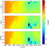 |
Fig. 15 Grid search ∆χ2 maps for Teff-log g (top panel), Teff-C/O (middle panel), and Teff−]Fe/H]. The solid, dashed, and dotted lines indicate 1, 2, and 3-σ confidence regions. The red cross indicates the optimum model. |
6.2 An MCMC sampling of models
We used emcee (Foreman-Mackey et al. 2013) to apply 1 000 000 iterations of a Markov chain Monte Carlo (MCMC) sampling around the best solution (found by gridsearch in Sect. 6.1) to assess the true posterior distribution and correlations among the varied parameters. The fitted physical parameters are Teff, log g, [Fe/H], C/O, vr, and v sin i. We also fit for the spectral resolving power Rspec, in order to account for possible deviations from R=4020 ± 30. We also sampled a rescaling, a, to adjust the continuum of model and observed spectra together. The preprocessings of data and models were the same as those used adopted in the gridsearch. The error bars of the data points, σdata, (as defined in Sect. 6.1) might be over or under estimated by a certain multiplicative amount ƒerr and under-estimated by a constant jitter σ. We thus use the error model  with σdata, depending on wavelength. We added ƒerr and σ as hyper-parameters in the MCMC. The prior distributions, either normal 𝒩 or uniform 𝒰, that we assumed for all parameters are listed in Table 3. All parameters, except Rspec, follow uniform priors.
The Exo-REM model spectra are interpolated through the initial 4D grid at the specific values of parameters chosen by the MCMC walkers at each new step. For a quick calculation, we applied the LinearNDInterpolator from scipy on the smallest Hull simplex, where each vertex is a model of the Exo-REM grid, surrounding each MCMC sampled point. This accounts for missing models at several grid nodes (see Sect. 4.1 above).
The MCMC runs for (at most) 1 000 000 steps with 20 walkers. It stops whenever the number of steps is smaller than 50× the largest auto-correlation length of the samples. Table 4 summarises the results of two different runs, one with all parameters freely varying within uninformed priors (except for R). The corner plot shows the posterior distributions with all parameters freely varying in Fig. A.1. The synthetic spectrum at the median of these posterior distributions is compared to the observed data on Fig. A.2. The derived parameters are in good agreement with the initial guess from the grid-search in Sect. 6.1 and lead to more reliable confidence regions, with an effective temperature ranging at 1-σ within  ,
,  , a super-solar
  , and a v sin i=31 ± 5 km s−1. Our temperature estimate agrees with the GRAVITY Collaboration (2020) results for the GRAVITY + GPIYJH band data fitted with exo-REM models (1590 ± 20 K). Also, our derived metallicity and log g values agree with the fit of the GRAVITY-only spectrum. However, we found a super-solar C/O; whereas those authors they found it to be sub-solar.
The log g∽3.1 result given above, as well as by the GRAVITY collaboration (GRAVITY Collaboration 2020), implies a planet mass close to 2 MJ. It disagrees with the independent dynamical constraints on the mass of the planet, namely, of ∽12 MJ (Snellen & Brown 2018; Lagrange et al. 2020; GRAVITY Collaboration 2020). We thus tried to fix the log g at a higher value, around 4.18, as suggested by Chilcote et al. (2017) work, defining a Gaussian prior probability distribution for the log g∽4.18 ± 0.01. As shown in Table 4, in this case, the MCMC leads to a larger temperature of  , and a smaller C/O of 0.551 ± 0.002 compatible with a solar value.
We also tried fixing the Teff prior to the Chilcote et al. (2017) value of 1724 ± 15 K, along with both log g and Teff. These trials are also shown in Table 4 and are compatible with the fixed-log g trial. We calculated the Akaike information criterion AIC=2k −2ln 𝓛 for all models. The maximum likelihood estimator (MLE) model obtained with the Teff fixed minimises the Akaike information criterion (AIC) and is thus preferred over all other models. The large difference in AIC of ∆AIC∽36 means that the Teff-fixed model is 2.5×10⁻⁸ times more likely than the model with uninformed priors, and 1.4× more likely than the model with both log g and Teff fixed. This preferred solution has a Teff of  , a log g=4.22 ± 0.03 (slightly larger than the Chilcote value of 4.18), a sub-solar
  , a solar C/O ∽0.551 ± 0.002, and a
  . In all cases, we found a jitter σ that is compatible with zero, with a correcting factor of error bars
  very close to 1. Both imply that our determination of flux error bars σdata introduced in Sect. 6.1 is reasonable. Figure 19 shows our preferred model compared to the observed planet spectrum and the corner plot of posterior distributions is shown in Fig. 18.
The radial velocity of the planet is found to be around 0.6 ± 0.9 km s−1 in the Earth reference frame. With a barycentric correction of 8.1 km s−1 this leads to a radial velocity of planet β Picb of 8.7 ± 0.9km s−1. Compared to β Pic systemic RV of −20 ± 0.7km s−1 (Gontcharov 2006), it implies an RV of the planet relative to β Pic’s central star of −11.3 ± 1.1 km s−1 at MJD=56910.38. This value agrees at 0.3–σ with the predicted RV of the planet at this MJD extrapolating the ephemerides of β Pic b’s orbital motion from the RV+astro+imaging solution of Lacour et al. (2021) of −11.6 km s−1. It also compares well to the RV measured at high resolution using CRIRES a year earlier, −15.4 ± 1.7 km s−1 at MJD=56,644.5 (Snellen et al. 2014).
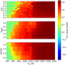 |
Fig. 16 Grid search CCF maps for Tefflog g (top panel) Teff-C/0 (middle panel), and Teff-]Fe/H]. The solid, dashed, and dotted lines indicate 1%, 10%, and 20% ∆CCF levels compared to the optimal CCF. The red cross indicates the optimum model. |
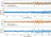 |
Fig. 17 Best-matching models, using the χ2 optimisation (top) and the CCF optimisation (bottom). |
Prior probability density functions (PDF) and parameters used for the MCMC runs.
MCMC results for the run.
7 Discussion
7.1 A new estimation of v sin i
In this work, we found a  in good agreement with the S14’s result v sin i=25 ± 3 km s−1 and the most recent Landman et al. (2023)’s v sin i estimation of 19.9 ± 1.1 km s−1. The larger confidence region of our measurement is explained by the much lower resolving power of SINFONI (R=4030 ± 30, as determined in Sect. 2.4) compared to that of CRIRES (R=75 000).
S14 noticed that given the mass of the planet, the spin velocity of 25 km s−1 was too low to comply with the log-linear mass-spin law followed by Solar System objects from Jupiter down to asteroids (e.g. Hughes 2003), which would imply a spin velocity of ∽50 km s−1. Figure 20 shows this relationship for the Solar System planets, with a log-linear law that is well fitted to Earth+Moon5, Mars, Jupiter, Saturn, Uranus, and Neptune mass and equatorial speed, with values taken from Hughes (2003). Mercury and Venus are recognised as deviating from this law due to a loss of momentum during their lifetimes through tidal interactions with the Sun (Fish 1967; Burns 1975; Hughes 2003).
The difference in v sin i for β Pic b compared to the expected equatorial speed at a mass of ∽11 MJ is mostly explained by the young age of the planet (∽23 Myr; Mamajek & Bell 2014). Indeed, the planet is currently contracting from ∽1.5 RJ down to ∽1 RJ (S14, Schwarz et al. 2016) and, thus, its spin should be accelerating. Figure 21 shows the effect of dilatation/contraction through time on the equatorial radius from two different evolution models: ATMO2020 (Phillips et al. 2020) and Baraffe-Chabrier-Barman (Baraffe et al. 2008). According to the conservation of momentum, its spin velocity is expected to increase up to 40 ± 20 km s−1 at 4.5Gyr, which is in better agreement with the Solar System law. Figure 22 shows the predicted v sin i at 23 Myr evolved backward using the ATMO2020 models, down from an equatorial velocity determined by the spin-mass law at 4.5 Gyr shown in Fig. 20. In Fig. 22, it can be seen that even when we are taking into account the contraction, there is still a tension between the v sin i measurements of β Pic b and its mass, especially if the mass is contained within 10–14 MJ. The v sin i and mass values overlap only over regions for v sin i>22 km s−1, with a mass of either <10 MJ or > 14 MJ. These masses are marginally supported by the combined astrometric and RV measurements that favour a planetary mass within 9–15 MJ (Dupuy et al. 2019; GRAVITY Collaboration 2020; Lagrange et al. 2020; Vandal et al. 2020; Brandt et al. 2021; Feng et al. 2022).
This remaining discrepancy between mass and v sin i could be explained by the random aspect of moment exchange during planet formation. However, it might also be the hint of a tilt of the planet’s equator compared to its orbital plane. In such case, the projected spin velocity, v sin i, is smaller than the true equatorial velocity. A direct compatibility at 1-σ of the predicted v sin i at 23 Myr for a mass at 11 MJ and our measurement 25 ± 6 km s−1 leads to a tilt compared to edge-on >15°.
 |
Fig. 18 Corner plot summarising the MCMC results for the fit of the β Pic b IR SINFONI spectrum by Exo-REM models with Teff fixed at the Chilcote et al. (2017) value (see text for details). |
7.2 A solar C/O
Here, we derive a value of the C/O for β Pic b that is Solar (0.551 ± 0.002), while GRAVITY Collaboration (2020) and Landman et al. (2023) found a sub-solar C/O of respectively 0.43 ± 0.05 and 0.41 ± 0.04. Forming β Pic b in situ along the core accretion scenario (Pollack et al. 1996) would imply a C/O ratio in the atmosphere of the planet largely super-solar >0.8, because of the expected abundances of the different gases in the disk from one ice line to the other when assuming a disk with a static composition all through the main phase of planet formation (Öberg et al. 2011). In this framework, a proposed scenario for reaching solar and sub-solar C/O is to consider the accretion of icy planetesimals from beyond the ice lines, where most of the H2O and CO2 of the disk is in condensed phase. Alternatively, a solar C/O is more naturally reached by forming either by gravitational instability (Boss 1997) anywhere in the disk or by core accretion close to the H2O ice line with a moderate planetesimal accretion followed by an outward migration. Given that core accretion is preferred for most compact planetary systems with also terrestrial planets (as in e.g. the Solar System) and that the β Pic system has at least two planets, with one within 5 au (Lagrange et al. 2019) plus small km-sized icy bodies (Ferlet et al. 1987; Beust et al. 1990; Kiefer et al. 2014; Lecavelier des Etangs et al. 2022), we further consider this scenario as the most likely for forming the β Pic’s planets.
In this framework, we can estimate the location of the ice lines compared to β Pic b location in the disk. Following Öberg et al. (2011), the typical temperature profile in a protoplanetary disk is given by (Andrews & Williams 2005, 2007):
 (11)
(11)
Here, T0 is the average temperature in the disk as if it were located at 1R★ from the centre of the star. Given the effective temperature of β Pic (Saffe et al. 2021), we have that T0=8000K. Considering the typical evaporation temperatures of H2O, CO2, and CO summarised in Table 5 with R★=1.7 R⊙ (Kervella et al. 2004), we derived the radii of the different ice lines around β Pic (also shown in Table 5). We find that with ab~9.8 au (Lagrange et al. 2020), planet b is located between the H2O (6±1 au) and the CO2 (31 ± 5 au) ice lines. Figure 23 shows the variation of the ice lines through time, as derived using Dartmouthl2 evolutionary tracks for pre-main sequence stars.
Following Petrus et al. (2021), our C/O measurement fits well to the Nissen (2013) planet-C/O to star-Fe/H linear relation. They indeed reported a positive correlation between the C/O ratio and the [Fe/H] of stars with an average C/O=0.58 ± 0.06 at [Fe/H]=0. Elemental abundances and spectral matching agree on a metallicity of β Pic that is solar up to a factor ~2 (Holweger et al. 1997). Our C/O of  is in good agreement with the expected solar C/O for a solar metallicity. The low metallicity of the planet that we found,
  , is also in agreement with new-generation planetary population synthesis (NGPPS, Schlecker et al. 2021) simulations through core-accretion, on the same range of semi-major axis ~10au, especially if the mass of β Pic b is larger than 10 MJ. The correlation between bulk metallicity and planet mass, as obtained through the NGPPS simulations performed around stellar hosts with metallicities ranging from −0.5 to 0.5, as seen in Fig. 10 of Petrus et al. (2021).
To explain the C/O value found when assuming a static disk composition during planet formation, as in Öberg et al. (2011), we propose that: i) planets b and c underwent an inner migration during the first Myr of their formation, allowing them to gather large amounts of gas with a solar composition; this is followed by ii) an outward migration, with planet b and c in a 7:1 mean motion resonance leading them to reach their actual location (Beust et al., priv. comm.). This scenario would allow us to avoid fine-tuning the icy planetesimal accretion within the planet to reach a nearly ideal solar C/O.
Alternatively, there is a scenario that does not require us to invoke an outward migration for β Pic b. Considering non-static disk composition, Mollière et al. (2022) found that pebble evaporation and the dilution of water and CO in-between the H2O and CO iceline (Fig. 6 in Mollière et al. 2022) can lead to a nearly stellar C/O ratio in the circumstellar gas in about 1 Myr. That could enable the in situ formation of β Pic b, provided most of its gas had not been accreted before 1 Myr.
In summary, a solar C/O for β Pic b is challenging for planet formation models. Interestingly, it fits into the mass-C/O relation obtained by Hoch et al. (2022). These authors found a clear threshold at 4 MJ, beyond which imaged planet mostly have C/O consistent with solar ~0.55; whereas below 4 MJ, a transiting planet a C/O value from 0.2 to 2.0. This threshold has been interpreted as distinguishing two main formation pathways for planets that are either less massive than 4 MJ and or more massive than 4 MJ. This 4-MJ threshold was already reported with respect to the distribution of stellar metallicities among massive giant exoplanets, offering a similar interpretation (Santos et al. 2017). Therefore, the solar C/O of β Pic b might be the sign of a formation scenario that differs from the usual core accretion scenario invoked for close-in less massive planets; namely, it still includes core accretion, but considering perhaps a distinct pathway for planets formed at large separation that did not undergo inward migration or, more simply, by gravitational instability.
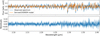 |
Fig. 19 Plot comparing in the top-panel the β Pic b SINFONI spectrum (blue) and the median Exo-REM model (orange) from the MCMC posteriors with Teff fixed at the Chilcote et al. (2017)’s value (see text). The bottom-panel shows the residuals. The uncertainties assumed for the observed flux are plotted as light-blue vertical lines. |
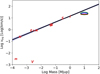 |
Fig. 20 Log-linear relationship between the equatorial velocity and mass of Solar System planets. In blue: possible laws compatible with planets Mars, lupiter, Saturn, Uranus, and Neptune. The ellipses show the v sin ì and mass of β Pic b derived in this work (pink), in S14 (cyan), and Landman et al. (2023, red). |
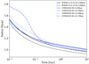 |
Fig. 21 Illustration of evolutionary tracks of equatorial radius through time with ATMO2020 models (Phillips et al. 2020) and Baraffe– Chabrier–Barman (Baraffe et al. 2008) or BCB08 models at different planet mass. |
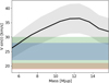 |
Fig. 22 v sin i prediction (gray region and black solid line) of the planet for different masses at 23 Myr, assuming a tilt of 0° compared to edge-on. Green and blue area show the v sin i confidence regions on β Pic b based on this work and the results from S14 (blue) and (Landman et al. 2023; red). |
Ice lines of CO, CO2, and H2O.
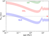 |
Fig. 23 Ice lines locations through time of H2O, CO2, and CO derived for β Pictoris. The location of planet b is marked as a red circle at 23 ± 3 Myr and prolonged down to 10 kyr with a black dotted line. |
8 Conclusion
In this study, we have derived a new infrared spectrum of the young giant planet β Pic b observed with SINFONI. We have shown that the actual spectral resolving power of SINFONI in the K-band at a spaxel-resolution of 12.5×25 mas2 is ~4000. Then, using a novel method of stellar halo removal, we have been able to directly extract the spectrum and the molecular lines of the planet without the need of using molecular mapping techniques. We have fitted the spectrum to models from the forward-modeling Exo-REM library. This has led to different results, depending on assumptions on the planet mass and radius:
without any prior constraints, we obtained
 at a
at a  , with a sub-solar metallicity of
  and a super-solar
  ;
;assuming a prior on the Teff =1724 ± 15 K, based on an independent photometric characterisation from Chilcote et al. (2017), we found a higher
 , again with a sub-solar metallicity of
  and a now solar C/O=0.551 ± 0.002.
Our preferred parameters were derived imposing Teff =1724 ± 15 K, as this better reflects the gravitational mass and the geometric radius derived independently using photometry. We found a projected rotation speed of β Pic b’s equator of  agreeing with the 25 ± 3 km s−1 found by Snellen et al. (2014) at high spectral resolution with CRIRES and the most recent CRIRES+ Landman et al. (2023)’s v sin i=19.9 ± 1.1 km s−1. However, our measurement of a solar C/O is in stark contrast with the sub-solar C/O-0.45 obtained from GRAVITY spectra (GRAVITY Collaboration 2020) and by the atmospheric retrieval of CRIRES spectra in Landman et al. (2023).
Conversely to the conclusions of GRAVITY Collaboration (2020), with a C/O for the star also close to 0.55, the stellar C/O disfavours the scenario of icy-planetesimals injection. It would indeed imply the need to fine-tune the planetesimals’ accretion flux and of the duration of the phenomenon, so that it reaches a value close to the stellar C/O. Such a value of β Pic b’s C/O is, on the other hand, in better agreement with in situ gravitational instability scenario or formation next to the H2O ice line, followed by migration. This latter scenario could be supported by the proximity of the planets b & c orbital periods to a 7:1 resonance, whose orbital parameters may have significantly evolved during the first Myrs of the system.
Finally, we measured a radial velocity of β Pic b relative to the central star of −11.3 ± 1.1 km s−1 at MJD=56,910.38. This is in agreement, at 0.3-σ, with the ephemerides for the orbit of this planet based on the current knowledge of the system from (Lacour et al. 2021). This tends to confirm the current estimation of the orbits and mass of the β Pic’s planets, while adding a new RV point for future dynamical characterisations of the system.
The present work shows that ground-based infrared medium-resolution spectroscopy with even a modest resolving power of 4000 (close to that of the JWST/MIRI-MRS) without the need to carry out molecular mapping and with a careful treatment of wavelength calibration, as well as star halo and telluric lines subtraction at any wavelengths. This can allow for the derivation of key properties of imaged exoplanets, including the equatorial rotation velocity. Proper determinations of the atmospheric parameters still requires independent priors, such as on Teff or log g, due to the fit degeneracy of the unresolved spectral lines.
Acknowledgements
We are thankful to Alain Smette for his careful and constructive reading of the manuscript that helped improving the analysis significantly. This work was granted access to the HPC resources of MesoPSL financed by the Region Ile de France and the project EquipMeso (reference ANR-10-EQPX-29-01) of the programme Investissements d'Avenir supervised by the Agence Nationale pour la Recherche. This project has received funding from the European Research Council (ERC) under the European Union s Horizon 2020 research and innovation programme (COBREX; grant agreement no. 885593). This work was also funded by the initiative de recherches interdisciplinaires et stratégiques (IRIS) of Université PSL “Origines et Conditions d’Apparition de la Vie (OCAV)”. F.K. also acknowledges funding from the Action Incitative Exoplanètes de l’Observatoire de Paris.
Appendix A MCMC run with all free parameters
 |
Fig. A.1 Corner plot summarising the MCMC results for the fit of the β Pic b IR SINFONI spectrum by Exo-REM models with all free parameters. The blue lines and dot show the median parameters. The orange lines and dot are those found for the preferred solution (see Section 6.2). |
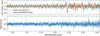 |
Fig. A.2 Plot comparing the β Pic b SINFONI spectrum (blue) and the median Exo-REM model (orange) from the MCMC posteriors (Fig. A.1). The lower panel shows the residuals. The uncertainties assumed for the observed flux are plotted as light-blue vertical lines. |
References
- Andrews, S. M., & Williams, J. P. 2005, ApJ, 631, 1134 [Google Scholar]
- Andrews, S. M., & Williams, J. P. 2007, ApJ, 659, 705 [NASA ADS] [CrossRef] [Google Scholar]
- Asplund, M., Grevesse, N., Sauval, A. J., & Scott, P. 2009, ARA&A, 47, 481 [NASA ADS] [CrossRef] [Google Scholar]
- Baraffe, I., Chabrier, G., & Barman, T. 2008, A&A, 482, 315 [NASA ADS] [CrossRef] [EDP Sciences] [Google Scholar]
- Baudino, J. L., Bézard, B., Boccaletti, A., et al. 2015, A&A, 582, A83 [NASA ADS] [CrossRef] [EDP Sciences] [Google Scholar]
- Beust, H., Lagrange-Henri, A. M., Vidal-Madjar, A., & Ferlet, R. 1990, A&A, 236, 202 [NASA ADS] [Google Scholar]
- Birkby, J. L., de Kok, R. J., Brogi, M., et al. 2013, MNRAS, 436, L35 [Google Scholar]
- Birkby, J. L., de Kok, R. J., Brogi, M., Schwarz, H., & Snellen, I. A. G. 2017, AJ, 153, 138 [NASA ADS] [CrossRef] [Google Scholar]
- Blain, D., Charnay, B., & Bézard, B. 2021, A&A, 646, A15 [EDP Sciences] [Google Scholar]
- Bonnefoy, M., Boccaletti, A., Lagrange, A. M., et al. 2013, A&A, 555, A107 [NASA ADS] [CrossRef] [EDP Sciences] [Google Scholar]
- Bonnet, H., Abuter, R., Baker, A., et al. 2004, The Messenger, 117, 17 [NASA ADS] [Google Scholar]
- Boss, A. P. 1997, Science, 276, 1836 [Google Scholar]
- Brandt, G. M., Brandt, T. D., Dupuy, T. J., Li, Y., & Michalik, D. 2021, AJ, 161, 179 [NASA ADS] [CrossRef] [Google Scholar]
- Brogi, M., Snellen, I. A. G., de Kok, R. J., et al. 2012, Nature, 486, 502 [Google Scholar]
- Brogi, M., Snellen, I. A. G., de Kok, R. J., et al. 2013, ApJ, 767, 27 [NASA ADS] [CrossRef] [Google Scholar]
- Brogi, M., de Kok, R. J., Birkby, J. L., Schwarz, H., & Snellen, I. A. G. 2014, A&A, 565, A124 [NASA ADS] [CrossRef] [EDP Sciences] [Google Scholar]
- Brogi, M., Giacobbe, P., Guilluy, G., et al. 2018, A&A, 615, A16 [NASA ADS] [CrossRef] [EDP Sciences] [Google Scholar]
- Burns, J. A. 1975, Icarus, 25, 545 [NASA ADS] [CrossRef] [Google Scholar]
- Charnay, B., Bézard, B., Baudino, J. L., et al. 2018, ApJ, 854, 172 [Google Scholar]
- Chilcote, J., Pueyo, L., De Rosa, R. J., et al. 2017, AJ, 153, 182 [Google Scholar]
- Cont, D., Yan, F., Reiners, A., et al. 2021, A&A, 651, A33 [NASA ADS] [CrossRef] [EDP Sciences] [Google Scholar]
- Cont, D., Yan, F., Reiners, A., et al. 2022a, A&A, 668, A53 [NASA ADS] [CrossRef] [EDP Sciences] [Google Scholar]
- Cont, D., Yan, F., Reiners, A., et al. 2022b, A&A, 657, L2 [NASA ADS] [CrossRef] [EDP Sciences] [Google Scholar]
- Cugno, G., Patapis, P., Stolker, T., et al. 2021, A&A, 653, A12 [NASA ADS] [CrossRef] [EDP Sciences] [Google Scholar]
- de Kok, R. J., Brogi, M., Snellen, I. A. G., et al. 2013, A&A, 554, A82 [NASA ADS] [CrossRef] [EDP Sciences] [Google Scholar]
- Demars, D., Bonnefoy, M., Dougados, C., et al. 2023, A&A 676, A123 [NASA ADS] [CrossRef] [EDP Sciences] [Google Scholar]
- Dupuy, T. J., Brandt, T. D., Kratter, K. M., & Bowler, B. P. 2019, ApJ, 871, L4 [Google Scholar]
- Eisenhauer, F., Abuter, R., Bickert, K., et al. 2003, SPIE Conf. Ser., 4841, 1548 [Google Scholar]
- Feng, F., Butler, R. P., Vogt, S. S., et al. 2022, ApJS, 262, 21 [NASA ADS] [CrossRef] [Google Scholar]
- Ferlet, R., Hobbs, L. M., & Vidal-Madjar, A. 1987, A&A, 185, 267 [NASA ADS] [Google Scholar]
- Fish, F. F. 1967, Icarus, 7, 251 [NASA ADS] [CrossRef] [Google Scholar]
- Foreman-Mackey, D., Hogg, D. W., Lang, D., & Goodman, J. 2013, PASP, 125, 306 [Google Scholar]
- Gontcharov, G. A. 2006, Astron. Astrophys. Trans., 25, 145 [NASA ADS] [CrossRef] [Google Scholar]
- GRAVITY Collaboration (Nowak, M., et al.) 2020, A&A, 633, A110 [NASA ADS] [CrossRef] [EDP Sciences] [Google Scholar]
- Gray, D. F. 1997, High resolution spectroscopy, in Instrumentation for large telescopes, 163 [CrossRef] [Google Scholar]
- Guilluy, G., Sozzetti, A., Brogi, M., et al. 2019, A&A, 625, A107 [NASA ADS] [CrossRef] [EDP Sciences] [Google Scholar]
- Hoch, K. K. W., Konopacky, Q. M., Theissen, C. A., et al. 2023, ApJ, 166, 85 [CrossRef] [Google Scholar]
- Hoeijmakers, H. J., Schwarz, H., Snellen, I. A. G., et al. 2018, A&A, 617, A144 [NASA ADS] [CrossRef] [EDP Sciences] [Google Scholar]
- Holweger, H., Hempel, M., van Thiel, T., & Kaufer, A. 1997, A&A, 320, L49 [NASA ADS] [Google Scholar]
- Hughes, D. W. 2003, Planet. Space Sci., 51, 517 [NASA ADS] [CrossRef] [Google Scholar]
- Kausch, W., Noll, S., Smette, A., et al. 2015, A&A, 576, A78 [NASA ADS] [CrossRef] [EDP Sciences] [Google Scholar]
- Kervella, P., Thévenin, F., Morel, P., et al. 2004, in Stars as Suns: Activity, Evolution and Planets, eds. A. K. Dupree, & A. O. Benz, 219, 80 [NASA ADS] [Google Scholar]
- Kervella, P., Arenou, F., Mignard, F., & Thévenin, F. 2019, A&A, 623, A72 [NASA ADS] [CrossRef] [EDP Sciences] [Google Scholar]
- Kervella, P., Arenou, F., & Thévenin, F. 2022, A&A, 657, A7 [NASA ADS] [CrossRef] [EDP Sciences] [Google Scholar]
- Kiefer, F., Lecavelier des Etangs, A., Boissier, J., et al. 2014, Nature, 514, 462 [Google Scholar]
- Lacour, S., Wang, J. J., Rodet, L., et al. 2021, A&A, 654, A2 [NASA ADS] [CrossRef] [EDP Sciences] [Google Scholar]
- Lagrange, A. M., Gratadour, D., Chauvin, G., et al. 2009, A&A, 493, L21 [NASA ADS] [CrossRef] [EDP Sciences] [Google Scholar]
- Lagrange, A. M., Bonnefoy, M., Chauvin, G., et al. 2010, Science, 329, 57 [Google Scholar]
- Lagrange, A. M., Boccaletti, A., Milli, J., et al. 2012, A&A, 542, A40 [NASA ADS] [CrossRef] [EDP Sciences] [Google Scholar]
- Lagrange, A. M., Meunier, N., Rubini, P., et al. 2019, Nat. Astron., 3, 1135 [NASA ADS] [CrossRef] [Google Scholar]
- Lagrange, A. M., Rubini, P., Nowak, M., et al. 2020, A&A, 642, A18 [NASA ADS] [CrossRef] [EDP Sciences] [Google Scholar]
- Landman, R., Stolker, T., Snellen, I., et al. 2023, A&A, 682, A48 [Google Scholar]
- Lecavelier des Etangs, A., Cros, L., Hébrard, G., et al. 2022, Sci. Rep., 12, 5855 [NASA ADS] [CrossRef] [Google Scholar]
- Lockwood, A. C., Johnson, J. A., Bender, C. F., et al. 2014, ApJ, 783, L29 [Google Scholar]
- Mâlin, M., Boccaletti, A., Charnay, B., Kiefer, F., & Bézard, B. 2023, A&A, 671, A109 [NASA ADS] [CrossRef] [EDP Sciences] [Google Scholar]
- Mamajek, E. E., & Bell, C. P. M. 2014, MNRAS, 445, 2169 [Google Scholar]
- Marois, C., Lafrenière, D., Doyon, R., Macintosh, B., & Nadeau, D. 2006, ApJ, 641, 556 [Google Scholar]
- Mesa, D., Gratton, R., Kervella, P., et al. 2023, A&A, 672, A93 [NASA ADS] [CrossRef] [EDP Sciences] [Google Scholar]
- Miles, B. E., Biller, B. A., Patapis, P., et al. 2023, ApJ, 946, L6 [NASA ADS] [CrossRef] [Google Scholar]
- Mollière, P., Molyarova, T., Bitsch, B., et al. 2022, ApJ, 934, 74 [CrossRef] [Google Scholar]
- Morzinski, K. M., Males, J. R., Skemer, A. J., et al. 2015, ApJ, 815, 108 [NASA ADS] [CrossRef] [Google Scholar]
- Nissen, P. E. 2013, A&A, 552, A73 [NASA ADS] [CrossRef] [EDP Sciences] [Google Scholar]
- Nowak, M., Lacour, S., Lagrange, A. M., et al. 2020, A&A, 642, A2 [NASA ADS] [CrossRef] [EDP Sciences] [Google Scholar]
- Öberg, K. I., Murray-Clay, R., & Bergin, E. A. 2011, ApJ, 743, L16 [Google Scholar]
- Palma-Bifani, P., Chauvin, G., Bonnefoy, M., et al. 2023, A&A, 670, A90 [NASA ADS] [CrossRef] [EDP Sciences] [Google Scholar]
- Patapis, P., Nasedkin, E., Cugno, G., et al. 2022, A&A, 658, A72 [NASA ADS] [CrossRef] [EDP Sciences] [Google Scholar]
- Petit dit de la Roche, D. J. M., Hoeijmakers, H. J., & Snellen, I. A. G. 2018, A&A, 616, A146 [EDP Sciences] [Google Scholar]
- Petrus, S., Bonnefoy, M., Chauvin, G., et al. 2021, A&A, 648, A59 [EDP Sciences] [Google Scholar]
- Petrus, S., Chauvin, G., Bonnefoy, M., et al. 2023, A&A, 670, A9 [NASA ADS] [CrossRef] [EDP Sciences] [Google Scholar]
- Phillips, M. W., Tremblin, P., Baraffe, I., et al. 2020, A&A, 637, A38 [NASA ADS] [CrossRef] [EDP Sciences] [Google Scholar]
- Piskorz, D., Benneke, B., Crockett, N. R., et al. 2016, ApJ, 832, 131 [NASA ADS] [CrossRef] [Google Scholar]
- Piskorz, D., Benneke, B., Crockett, N. R., et al. 2017, AJ, 154, 78 [NASA ADS] [CrossRef] [Google Scholar]
- Pollack, J. B., Hubickyj, O., Bodenheimer, P., et al. 1996, Icarus, 124, 62 [NASA ADS] [CrossRef] [Google Scholar]
- Ruffio, J.-B., Macintosh, B., Konopacky, Q. M., et al. 2019, AJ, 158, 200 [Google Scholar]
- Ruffio, J.-B., Konopacky, Q. M., Barman, T., et al. 2021, AJ, 162, 290 [NASA ADS] [CrossRef] [Google Scholar]
- Saffe, C., Miquelarena, P., Alacoria, J., et al. 2021, A&A, 647, A49 [NASA ADS] [CrossRef] [EDP Sciences] [Google Scholar]
- Santos, N. C., Adibekyan, V., Figueira, P., et al. 2017, A&A, 603, A30 [NASA ADS] [CrossRef] [EDP Sciences] [Google Scholar]
- Schlecker, M., Mordasini, C., Emsenhuber, A., et al. 2021, A&A, 656, A71 [NASA ADS] [CrossRef] [EDP Sciences] [Google Scholar]
- Schwarz, H., Ginski, C., de Kok, R. J., et al. 2016, A&A, 593, A74 [NASA ADS] [CrossRef] [EDP Sciences] [Google Scholar]
- Skilling, J. 2006, Bayesian Anal., 1, 833 [Google Scholar]
- Smette, A., Sana, H., Noll, S., et al. 2015, A&A, 576, A77 [NASA ADS] [CrossRef] [EDP Sciences] [Google Scholar]
- Snellen, I. A. G., & Brown, A. G. A. 2018, Nat. Astron., 2, 883 [Google Scholar]
- Snellen, I. A. G., Brandl, B. R., de Kok, R. J., et al. 2014, Nature, 509, 63 [Google Scholar]
- Tamuz, O., Mazeh, T., & Zucker, S. 2005, MNRAS, 356, 1466 [Google Scholar]
- Vandal, T., Rameau, J., & Doyon, R. 2020, AJ, 160, 243 [NASA ADS] [CrossRef] [Google Scholar]
- Yan, F., Pallé, E., Reiners, A., et al. 2022, A&A, 661, A6 [NASA ADS] [CrossRef] [EDP Sciences] [Google Scholar]
The commonly adopted solar abundance values are log NM,⊙/NM,⊙=log Z⊙/X⊙=−1.74 and C/O=0.55 (Asplund et al. 2009).
Spaxel-to-spaxel variations in the telluric spectrum arise from small differences in the wavelength calibration from one spaxel to the others, and from adding a non-zero spaxel-dependent background continuum when fitting and subtracting the reference stellar (plus telluric) spectrum in Sect. 3.2.
Due to major exchange of momentum between Earth and Moon, the Earth+Moon couple is considered as if the Moon was put back into the Earth and the total momentum conserved (Hughes 2003).
All Tables
Comparing results of the different star spectrum subtraction schemes on the normalised CCF of the residual map with a 1700 K, log g=4.0, [Fe/H]=0.0 Exo-REM model, detailing the CO and H2O individual contributions.
All Figures
|
Fig. 1 Absolute total (blue) and residual (orange) flux per spaxel. The spaxels are ordered from the brightest to the faintest in absolute total flux per spaxel. The absolute total flux is the raw flux obtained as output of the stack phase in Sect. 2.5. The residual flux is the remaining absolute flux once the star spectrum is removed (see Sect. 3.2 for more details). |
| In the text | |
|
Fig. 2 Star spectrum calculated from the brightest spaxels. The flux is normalised to the pseudo-continuum flux at the top of the Br-γ line at 2.165 µm. |
| In the text | |
|
Fig. 3 Summary of molecfit results. First panel: wavelength solutions showing the Doppler shift against the wavelength through the K-band with respect to cubes series number. Second panel: measured resolving power from FWHM of the fitted LSF. Third and fourth panels: fitted ppmv abundances of H2O, CO2, CH4, and N2O. |
| In the text | |
|
Fig. 4 Stellar spectrum observed with SINFONI (blue) compared to the model Earth telluric spectrum calculated with molecfit (orange) and the continuum model (green). Upper panel: two spectra compared directly. Lower panel: stellar spectrum divided by the telluric spectrum model. |
| In the text | |
|
Fig. 5 Steps of star spectrum removal methods compared. Qobs stands for the stacked cube observed, while |
| In the text | |
|
Fig. 6 Raw β Pic b spectrum extracted from the planet spaxels after using H18 method of star light removal. SYSREM was not used here. We highlight in red the main artefact that is due to excess star spectrum lines removal at the Brackett-γ wavelength. We also note that since the continuum has been subtracted, the reference level to which compare the strength of planet molecular lines (CO shown in green) is missing. |
| In the text | |
|
Fig. 7 Star flux fraction, |
| In the text | |
|
Fig. 8 Warp function δK(λ) (orange) normalised to 1 at the Brackett-γ wavelength (top panel), compared to a normalised Exo-REM model with T=1750K, logg = 4.0, [Fe/H]=0.0, and C/O=0.55 (blue) as well as the normalised stellar spectrum |
| In the text | |
|
Fig. 9 Background-subtraction and telluric removal from a planet-spaxel spectrum. Top: planet spaxel spectrum and average background on a distant ring. Middle: ηres,corr compared to its fitted telluric model ηtell. Bottom: planet-spaxel spectrum corrected from background and tellurics. |
| In the text | |
|
Fig. 10 Histogram of relative difference between the exo-REM models emittance and Stefan-Boltzman law. |
| In the text | |
|
Fig. 11 SINFONI planet absorption spectrum of β Pic b along the K-band, once corrected from star, background, and telluric pollutions (top). Exo-REM spectrum of simulated atmosphere of 1700 K, log(g)=4.0, and [Fe/H]=0.0 with R=6000 (bottom). Individual contributions of species CO, H2O, CH4, and NH3 are represented from top to bottom with diverse colors. For all the spectra, their continuum were divided, as explained in Sect. 4.2. |
| In the text | |
|
Fig. 12 Molecular CCF maps of β Pic b for species CO, H2O, CH4 (10−4) and NH3 (10−4). At each spaxel, the maps show the CCF height at 0 km s−1, a value close to the expected radial velocity of the planet b, |VR|<10 km s−1 given the instrument LSF of ~75 km s−1. |
| In the text | |
|
Fig. 13 Planet PSF radial profile at a varying distance from 0 to 8 spax-els. The relative flux is obtained by dividing out the continuum and subtracting the star spectrum, as explained in Sect. 3.2. |
| In the text | |
|
Fig. 14 Background removal. Top panel: average spectrum about the planet centroid (blue) compared to the average background spectrum on a ring around the planet (orange). Common features can be well distinguished. Bottom panel: planet spectrum corrected from the background. The features remaining are β Picb’s atmosphere absorption lines, while the main stellar feature (Brackett-γ) has been fully removed. |
| In the text | |
|
Fig. 15 Grid search ∆χ2 maps for Teff-log g (top panel), Teff-C/O (middle panel), and Teff−]Fe/H]. The solid, dashed, and dotted lines indicate 1, 2, and 3-σ confidence regions. The red cross indicates the optimum model. |
| In the text | |
|
Fig. 16 Grid search CCF maps for Tefflog g (top panel) Teff-C/0 (middle panel), and Teff-]Fe/H]. The solid, dashed, and dotted lines indicate 1%, 10%, and 20% ∆CCF levels compared to the optimal CCF. The red cross indicates the optimum model. |
| In the text | |
|
Fig. 17 Best-matching models, using the χ2 optimisation (top) and the CCF optimisation (bottom). |
| In the text | |
|
Fig. 18 Corner plot summarising the MCMC results for the fit of the β Pic b IR SINFONI spectrum by Exo-REM models with Teff fixed at the Chilcote et al. (2017) value (see text for details). |
| In the text | |
|
Fig. 19 Plot comparing in the top-panel the β Pic b SINFONI spectrum (blue) and the median Exo-REM model (orange) from the MCMC posteriors with Teff fixed at the Chilcote et al. (2017)’s value (see text). The bottom-panel shows the residuals. The uncertainties assumed for the observed flux are plotted as light-blue vertical lines. |
| In the text | |
|
Fig. 20 Log-linear relationship between the equatorial velocity and mass of Solar System planets. In blue: possible laws compatible with planets Mars, lupiter, Saturn, Uranus, and Neptune. The ellipses show the v sin ì and mass of β Pic b derived in this work (pink), in S14 (cyan), and Landman et al. (2023, red). |
| In the text | |
|
Fig. 21 Illustration of evolutionary tracks of equatorial radius through time with ATMO2020 models (Phillips et al. 2020) and Baraffe– Chabrier–Barman (Baraffe et al. 2008) or BCB08 models at different planet mass. |
| In the text | |
|
Fig. 22 v sin i prediction (gray region and black solid line) of the planet for different masses at 23 Myr, assuming a tilt of 0° compared to edge-on. Green and blue area show the v sin i confidence regions on β Pic b based on this work and the results from S14 (blue) and (Landman et al. 2023; red). |
| In the text | |
|
Fig. 23 Ice lines locations through time of H2O, CO2, and CO derived for β Pictoris. The location of planet b is marked as a red circle at 23 ± 3 Myr and prolonged down to 10 kyr with a black dotted line. |
| In the text | |
|
Fig. A.1 Corner plot summarising the MCMC results for the fit of the β Pic b IR SINFONI spectrum by Exo-REM models with all free parameters. The blue lines and dot show the median parameters. The orange lines and dot are those found for the preferred solution (see Section 6.2). |
| In the text | |
|
Fig. A.2 Plot comparing the β Pic b SINFONI spectrum (blue) and the median Exo-REM model (orange) from the MCMC posteriors (Fig. A.1). The lower panel shows the residuals. The uncertainties assumed for the observed flux are plotted as light-blue vertical lines. |
| In the text | |
Current usage metrics show cumulative count of Article Views (full-text article views including HTML views, PDF and ePub downloads, according to the available data) and Abstracts Views on Vision4Press platform.
Data correspond to usage on the plateform after 2015. The current usage metrics is available 48-96 hours after online publication and is updated daily on week days.
Initial download of the metrics may take a while.