| Issue |
A&A
Volume 675, July 2023
|
|
|---|---|---|
| Article Number | A157 | |
| Number of page(s) | 16 | |
| Section | Planets and planetary systems | |
| DOI | https://doi.org/10.1051/0004-6361/202245169 | |
| Published online | 14 July 2023 | |
Trade-offs in high-contrast integral field spectroscopy for exoplanet detection and characterisation
Young gas giants in emission
1
Leiden Observatory, Leiden University,
Postbus 9513,
2300
RA Leiden,
The Netherlands
e-mail: rlandman@strw.leidenuniv.nl
2
Lowell Observatory,
1400 W Mars Hill Rd,
Flagstaff AZ
86001,
USA
3
Université Côte d’Azur, Observatoire de la Côte d’Azur, CNRS, Laboratoire Lagrange,
06108
Nice,
France
4
Université Grenoble Alpes, CNRS, IPAG,
38000
Grenoble,
France
5
Max Planck Institute for Astronomy,
Königstuhl 17,
69117
Heidelberg,
Germany
Received:
7
October
2022
Accepted:
17
May
2023
Context. Combining high-contrast imaging with medium- or high-resolution integral field spectroscopy has the potential to boost the detection rate of exoplanets, especially at small angular separations. Furthermore, it immediately provides a spectrum of the planet that can be used to characterise its atmosphere. The achievable spectral resolution, wavelength coverage, and FOV of such an instrument are limited by the number of available detector pixels.
Aims. We aim to study the effect of the spectral resolution, wavelength coverage, and FOV on the detection and characterisation potential of medium- to high-resolution integral field spectrographs with molecule mapping.
Methods. The trade-offs are studied through end-to-end simulations of a typical high-contrast imaging instrument, analytical considerations, and atmospheric retrievals. The results are then validated with archival VLT/SINFONI data of the planet β Pictoris b.
Results. We show that molecular absorption spectra generally have decreasing power towards higher spectral resolution and that molecule mapping is already powerful for moderate resolutions (R ≳ 300). When choosing between wavelength coverage and spectral resolution for a given number of spectral bins, it is best to first increase the spectral resolution until R ~ 2000 and then maximise the bandwidth within an observing band. We find that T-type companions are most easily detected in the J/H band through methane and water features, while L-type companions are best observed in the H/K band through water and CO features. Such an instrument does not need to have a large FOV, as most of the gain in contrast is obtained in the speckle-limited regime close to the star. We show that the same conclusions are valid for the constraints on atmospheric parameters such as the C/O ratio, metallicity, surface gravity, and temperature, while higher spectral resolution (R ≳ 10 000) is required to constrain the radial velocity and spin of the planet.
Key words: planets and satellites: detection / techniques: imaging spectroscopy / instrumentation: high angular resolution / planets and satellites: atmospheres / planets and satellites: gaseous planets
© The Authors 2023
 Open Access article, published by EDP Sciences, under the terms of the Creative Commons Attribution License (https://creativecommons.org/licenses/by/4.0), which permits unrestricted use, distribution, and reproduction in any medium, provided the original work is properly cited.
This article is published in open access under the Subscribe to Open model. Subscribe to A&A to support open access publication.
1 Introduction
Direct imaging of exoplanets provides an ideal way to study their atmospheres and orbital configurations (Bowler 2016). These observations are technically challenging, as they require overcoming a large contrast between a bright star and a dim exoplanet at a small angular separation. This can be achieved through a combination of extreme adaptive optics (XAO), coro-nagraphy, and post-processing. Imaging surveys with dedicated high-contrast imaging instruments on 8-m class telescopes, such as SPHERE (Beuzit et al. 2019), GPI (Macintosh et al. 2014) and SCExAO (Jovanovic et al. 2015), have resulted in the detection of a few dozen planetary and brown dwarf companions (e.g. Macintosh et al. 2015; Konopacky et al. 2016; Chauvin et al. 2017; Milli et al. 2017; Keppler et al. 2018; Cheetham et al. 2018; Currie et al. 2020, 2022; Bohn et al. 2020, 2021). These surveys have mostly been sensitive to young, wide-orbit planets that are still luminous from their formation. While the surveys provide constraints on the demographics of these widely separated planets (Nielsen et al. 2019; Vigan et al. 2021), these companions appear to be relatively rare. To probe the bulk of the giant planet population, we need to increase the contrast, especially at smaller angular separations. However, most of the currently used post-processing techniques, such as angular differential imaging (ADI) and spectral differential imaging (SDI) perform poorly at small angular separations, <0.2″ (Marois et al. 2006; Rameau et al. 2015). These algorithms fundamentally suffer from this limitation because the amount of diversity decreases with a smaller angular separation.
In contrast, high-dispersion spectroscopy can detect thermal emission from both transiting and non-transiting exoplanets with minimal spatial separation and starlight suppression by cross-correlating with planet-model spectra (e.g. Brogi et al. 2012; Snellen et al. 2014). This technique can use both the rapidly varying radial velocity of the planet as well as the distinct planetary spectral features to distinguish between the light of the planet and the star. High-dispersion spectroscopy has been used to detect molecules in exoplanet atmospheres (e.g. Birkby et al. 2013; de Kok et al. 2013; Brogi et al. 2014) and, for example, to estimate their spin (Snellen et al. 2014; Schwarz et al. 2016; Bryan et al. 2018; Wang et al. 2021). Sparks & Ford (2002) were the first to propose that the combination of high-contrast imaging with a medium to high spectral resolution integral field spectrograph (IFS) can improve our ability to detect exoplanets. The potential of this technique has been studied many times (Snellen et al. 2015; Riaud & Schneider 2007; Wang et al. 2017). While current high-contrast imagers only have low spectral resolution IFSs (R < 100), observations using instruments such as VLT/SINFONI, Keck/OSIRIS, and VLT/MUSE (R > 1000) have indeed demonstrated the potential of these techniques (Konopacky et al. 2013; Hoeijmakers et al. 2018; Haffert et al. 2019), even though those instruments were not designed for high-contrast imaging. Not only can such IFSs be used to boost the detection limits, but they can also simultaneously provide a moderate-resolution spectrum of the planet, thereby facilitating both detection and atmospheric characterisation with a single observation. Moderate-resolution emission spectra obtained using these instruments have been used to detect molecules (e.g. Konopacky et al. 2013; Barman et al. 2015; Petit dit de la Roche et al. 2018; Hoeijmakers et al. 2018), accretion tracers (Haffert et al. 2019; Eriksson et al. 2020), and even isotopes (Zhang et al. 2021). Furthermore, they can constrain the radial velocity (Ruffio et al. 2019) and atmospheric parameters, such as the C/O ratio and metallicity (e.g. Ruffio et al. 2021; Petrus et al. 2021; Wilcomb et al. 2020), thereby revealing information about the formation and migration history of the planet (Mollière et al. 2022).
These promising results have led to the development of multiple instruments that aim to combine high-contrast imaging and high-dispersion spectroscopy. These include the coupling of existing high-contrast imagers with high-dispersion spectro-graphs such as VLT/HIRISE (Vigan et al. 2018; Otten et al. 2021), Keck/KPIC (Jovanovic et al. 2019; Delorme et al. 2021), and Subaru/REACH (Jovanovic et al. 2017; Kotani et al. 2020). However, these instruments only use a single or a few fibers in the focal plane. If the position of the planet is known, they allow for detailed characterisation of the planets, as was done for the HR8799 planets in Wang et al. (2021). While new techniques are being developed to use such instruments for planet detection within the diffraction limit (Echeverri et al. 2020; Xin et al. 2022), these instruments generally do not allow for the search of unknown companions over a significant FOV. In such cases, a larger FOV needs to be sampled through an IFS. Promising upcoming instruments with such a capability are ERIS (Davies et al. 2018) and MedRes, the medium-resolution IFS for the planned upgrade of SPHERE (Boccaletti et al. 2020; Gratton et al. 2022). The arrival of the ELT, HARMONI (Thatte et al. 2021), and METIS (Brandl et al. 2021) will provide moderate or high spectral and high spatial resolution IFSs in the near- and mid-infrared, which will be well suited for the detection and characterisation of exoplanets (Houllé et al. 2021; Carlomagno et al. 2020). From space, moderate-resolution IFSs are provided by NIRSPEC-IFU and MIRI-MRS on board of the James Webb Space Telescope (Patapis et al. 2022).
These IFSs are inherently limited by their number of available detector pixels. For example, increasing the spectral resolution, spectral bandwidth, FOV, and spatial sampling would lead to an increase in the number of pixels that are required. It is not trivial to choose the optimum values for each of these parameters. Furthermore, in planning observations, it is not obvious if it is better to use the higher spectral resolution mode of an instrument or to have broader wavelength coverage. In this work, we study these trade-offs and the impact of the different parameters on the detection and characterisation of exoplanets. Section 2 provides details on the end-to-end simulations and spectral models, followed by the results in Sect. 3. We validate some of our simulation results with real observations using VLT/SINFONI in Sect. 4. Finally, in Sect. 5 we look at the characterisation potential of such an instrument. Future work will study how these trade-offs change if the main goal of the instrument is to detect exoplanets in reflected light, instead of emission, such as for the future Planetary Camera and Spectrograph (PCS) instrument at the ELT (Kasper et al. 2021).
2 Simulations
2.1 Instrument model
To study the various trade-offs, we simulated a typical high-contrast imaging instrument on an 8-metre telescope and used VLT/SPHERE (Beuzit et al. 2019) as an example. While our simulations were done for an 8-m class telescope, most of the trade-offs are also applicable to the integral field spectrographs in the near-infrared of future ELTs, such as HARMONI (Thatte et al. 2021) and PCS (Kasper et al. 2021). Our simulations were done using the obsim1 python package for end-to-end simulations (Fagginger-Auer, in prep.). This framework allowed for modular Fourier-based simulations of instrument concepts and observations and is built on top of HCIPy (Por et al. 2018).
Our mock instrument consists of the VLT aperture followed by an implementation of the Apodized Pupil Lyot Coronagraph (APLC; Soummer 2005; Martinez et al. 2009; N’Diaye et al. 2016), as currently present in VLT/SPHERE. The simulations of the APLC were validated against the Coronagraphs package for python (N’Diaye, priv. comm.). Instead of doing the full XAO simulations, as is done in Houllé et al. (2021), we used the reconstructed XAO wavefront errors, non-common path aberrations (NCPA), and amplitude errors obtained for SPHERE, as described in Appendix B in Vigan et al. (2019). The simulations were run wavelength by wavelength, resulting in a datacube with an image at each wavelength. We ran the simulations for 5000 frames of the reconstructed XAO residuals with a FOV (FOV) of 2″ in diameter and a spectral resolution of 30000, since it can later be resampled to lower spectral resolutions. The simulations were done in the J, H, and K bands, and the size of the focal plane mask of the APLC was for each band adopted to the values specified in Beuzit et al. (2019).
Since the simulation of the datacubes at this spectral resolution is very time consuming, we opted not to simulate the full cubes for the off-axis planets. Instead, we estimated the average throughput of the planet signal through the APLC as a function of separation in each band. The companion signal was then modelled as the non-coronagraphic datacube shifted to the location of the companion and scaled by the estimated throughput of the coronagraph. Additionally, we assumed a general instrument throughput of 5%, which is slightly below the estimated optimal throughput for a fiber-based IFS (Haffert et al. 2020). An example of the resulting collapsed noiseless cube with and without the coronagraph in the H-band is shown in Fig. 1.
2.2 Astrophysical models
In this paper, we studied three planets from archetypical, directly imaged planetary systems: β Pictoris b (Lagrange et al. 2010), 51 Eridani b (Macintosh et al. 2015), and HR8799 e (Marois et al. 2010). The assumed properties of these planets as used in the simulations are ppecified in Table 1. Furthermore, we assumed solar metcllicity and elemental abundcnces for all of them and a radial velocity of 20 km s−1 between the target and observer. The input emission spectra for these planets were obtained from the BT-SETTL grid of atmosphere models (Allard 2014), while the PHOENIX stellar models (Husser et al. 2013) were used for the stellar spectra.
2.3 Mock observations
We used the atmospheric transmission and sky emission from ESO’s SkyCalc tool (Noll et al. 2012) for an airmass of 1.1 and precipitable water vapour of 2.5 mm. We did not consider thermal emission from the instrument itself, which may start; to contribute in the K-band. The baseline simulations consist of 60 times 60 s exposures, and the flux in each wavelength bin in the cubes was scaled according to the expected number of received photons from the spectra and instrument properties.
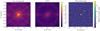 |
Fig. 1 Visualisation of the simulated datacubes. Left: resulting wavelength summed H-band images from the simulations described in Sect. 2.1. Middle: same but including am implementation of the APLC. Right: example result of me data analysis. The location of the planet is indicated with a red circle. |
Assumed parameters of the planetary systems used for the simulations throughout this paper.
2.4 Molecule mapping
Detecting a planet in the resulting datacubes can be done using the molecule mapping technique developed by Hoeijmakers et al. (2018). In this technique, the stellar and telluric contamination is removed from each spaxel, leaving the planet signal with noise. Subsequently, a matcaed fillter or cross-correlation is applied to the residuals. It there is uncorrelated Gaussian noise, the signal-to-noise ratio (S/N) of a matched filter is given by (Ruffio et al. 2017; Houllé et al. 2021):
 (1)
(1)
whece si is the observed data, ti the template, σi the uncertainties, and N the total number of data points. These data points, indexed by i, can be pixels spanning both the spectral domain (the planetary spectrum) and spatial domain (the shape of the Point Spread Function, or PSF), For the simulations, we knew the noise of each data point exactly, allowing us to directiy apply Eq. (1). The noise of a data point σi. is given by:
 (2)
(2)
Here,  ,
,  , and Fbg are refpectively the stellar, planet, and background contribution to the noise at the considered spaxel and spectral bin. These contributions to the noise were obtained from the simulated datacubes described in Sect. 2.1. The value of RON is the total readout noise of each spectral bin. For the baseline simulations, we assumed each spectral bin effectively covers two physical pixels on the detector and has a readout noise of 1 e− rms pixel−1 read−1.
We experimented with adding noise to the datacubes and then doing the full data analysis following Hoeijmakers et al. (2018) to estimate the S/N, and we found results equivalent to those of Eq. (1). To have consistency across the different instrument configurations and avoid dependency on the choice of the values of parameters of the algorithm, we have opted to only present the analytical results from Eq. (1), just as was done in Otten et al. (2021).
The matched filter templates ti used throughout this paper consist of the BT-SETTL spectra and molecular templates generated using petitRADTRANS (Mollière et al. 2019), convolved to the appropriate spectral resolution. Molecule mapping generally results in the loss of the continuum, and we therefore high-pass fiftered these tempiates. This was done by convolving the original templates with a Gaussian kernel with a standard deviation of 0.01 µm and subtracting this from the original spectrum. Examples of high-pass filtered templates are shown in Appendix A. For the spatial part of the matched filter, we used a Gaussian function with an appropriate full-width at half maximum (FWHM) given the wavelength.
3 Trade-off results
In this section, we study how different properties of the instrument impact its ability to detect new planets. This is be done based on analytical considerations and the simulations described in Sect. 2. The studied properties are the spectral resolution, spectral bandwidth, observing band, and FOV.
3.1 Spectral resolution
The impact of the spectral resolution on the S/N that can be achieved is not trivial. Increasing the spectral resolution leads to more data points for the matched filter (N ∝ R) but decreases the S/N per spectral bin. Furthermore, the observed spectrum also changes as a function of spectral resolution, as individual lines may start to be resolved and become deeper.
3.1.1 Power spectral density
We analysed the strength of the features that are resolved at a specific spectral resolution by looking at the power spectral density (PSD) of the planet spectrum tp. The PSD of a sequence tp(x) defined over a range L = xmax − xmin can be approximated by:
![$\matrix{ {PSD\left[ {{t_{\rm{p}}}\left( x \right)} \right]\left( f \right) = {1 \over L}{{\left| {{\cal F}\left[ {{t_{\rm{p}}}\left( x \right)} \right]} \right|}^2}} \hfill \cr {\,\,\,\,\,\,\,\,\,\,\,\,\,\,\,\,\,\,\,\,\,\,\,\,\,\,\,\,\,\,\,\, \approx {1 \over L}{{\left| {\int_{{x_{\min }}}^{{x_{\max }}} {{t_{\rm{p}}}} \left( x \right){{\rm{e}}^{ - i2\pi fx}}{\rm{d}}x} \right|}^2},} \hfill \cr } $](/articles/aa/full_html/2023/07/aa45169-22/aa45169-22-eq5.png) (3)
(3)
where ℱ is the Fourier transform operator, tp the considered planetary spectrum, and f the frequency of the corresponding fluctuation. This PSD can also be expressed in terms of the effective spectral resolution R′ using R′ = λ/(2Δλ′). We did this by sampling the planet spectrum logarithmically in wavelength (i.e. x = log λ), keeping the spectral resolution constant across the wavelength range. In this case, the conjugate variable in the Fourier domain is f ≈ λ/Δλ′ = 2R′ (see Appendix C). The factor two was added to account for the fact that we needed to Nyquist sample the spectrum to see fluctuations of a specific frequency. It is important to note that Δλ′ and R′ refer to the period and frequency of a fluctuation respectively and not the actual resolution element of the instrument. Using the definition of the PSD from above, we obtained:
![$\matrix{ {P\left( {R\prime } \right) \equiv {\rm{PSD}}\left[ {{t_{\rm{p}}}\left( {\log \lambda } \right)} \right]\left( {{f \mathord{\left/ {\vphantom {f 2}} \right. \kern-\nulldelimiterspace} 2}} \right)} \hfill \cr {\,\,\,\,\,\,\,\,\,\,\,\,\, \approx {1 \over L}{{\left| {\int_{\log {\lambda _{\min }}}^{\log {\lambda _{\max }}} {{t_{\rm{p}}}} \left( {\log \lambda } \right){{\rm{e}}^{ - i2\pi R\prime \,\log \,\lambda }}{\rm{d}}\log \lambda } \right|}^2},} \hfill \cr } $](/articles/aa/full_html/2023/07/aa45169-22/aa45169-22-eq6.png) (4)
(4)
with L = log λmax – log λmin. The normalised PSD of different contributions to the observed spectrum between 1 and 2.5 µm is shown in Fig. 2 as a function of effective spectral resolution. The PSDs were estimated using Welch’s method and smoothed for visibility purposes. The planet contributions presented here are for a HR8799e-like planet and are shown both with and without rotational broadening. The PSD’s of the other reference targets are shown in Appendix B. We also show the PSD for a single infinitely thin spectral line (δ-line) and white noise. Finally, because of the wavelength dependence of the PSF, stellar speckles shift outwards for increasing wavelengths. This imposes a low-order modulation to the stellar contribution to each spaxel and depends on the separation of the source and the present wavefront aberrations. Figure 2 also shows the average PSD of this speckle modulation, which we calculated in a square area between 2 and 7 λ/D from the simulated coronagraphic datacubes from Sect. 2.
Figure 2 shows that the modulation of stellar speckles is a low-order effect and has the most power at low spectral resolutions. The power of these fluctuations very quickly decreases at higher spectral resolution. This illustrates that applying a spectral high-pess filter is indeed very effective at removing stellar gontamination, as it leaves only narrow spectrat features such as stellar and telluric lines. Since these are shared between alt of the spaxels, they can often be removed using, for example, a principal component analysis (PCA; e.g. Hoeijmakers et al. 2018; Ruffio et al. 2021).
The PSD s of the molecular templates are mora complex. Figure 2 shows that the power generally decreases for higher spectral resolutions. This is the result of the band structure of the absorption spectra. Furthermore, at very high resolutions (R > 50 000), we also observed decreasing power due to the intrinsic broadening of the individual ro-vibrational lines. We also Sound that, mostly for (CO and CH4, there are clear peaks in the power spectrum. This is because of the ro-vibrational structure of the absorption features, which can have a specific periodicity and are therefore resolved at a specific spectral resolution. This is especially prominent for CO, which has a sawtooth structure in its bandheads. Finally, both a δ-line and white noise have a flat PSD and are the dominating contributors at the highest spectral resolutions. While the PSD of the molecular features depends slightly on the parameters of the planet, such as the temperature structure, the general trend is the same, as can be seen in Appendix B.
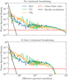 |
Fig. 2 Normalised PSD of different contributions to the observed spectrum between 1 and 2.5 µm. Here, we assumed a planet with an effective temperature of 1200 K and log(g) of 4.0. The panels show the results without rotational broadening (top) and with rotational broadening of υrot sin i = 15 km s−1 (bottom). |
3.1.2 Signal-to-noise ratio approximation
Next, we discuss the relation between the S/N and spectral resolution of the instrument. If we assume that we have a perfect match between the template t and the observed data s with some uncorrelated Gaussian noise ni = 𝒩(0, σi) we have
 (5)
(5)
simplifying Eq. (1) to:
 (6)
(6)
For simplicity, we assumed that the planet flux is concentrated in a single spaxel with M spectral bins. Further assuming that the noise in each spectral bin is roughly the same (σi ≈ σ), we could approximate this with:
 (7)
(7)
where < t2 > denotes the average of t2. From this equation, we could show the following relation between the matched filter S/N and the PSD (see Appendix C for the derivation):
 (8)
(8)
Here, P(R′) is the PSD of the planet spectrum as discussed in Sect. 3.1.1, and H(R′) is the transfer function describing the impact of the spectrograph, detector, and data reduction on the observed spectrum. Assuming an ideal Nyquist-sampled spectrograph that acts as an ideal low-pass filter up to the Nyquist frequency set by the spectral resolution R and that the data reduction functions as an ideal high-pass filter, removing all features below R′ = Rmin, we obtained the following equation (see Appendix C for details):
 (9)
(9)
where we have used M = 2BR for Nyquist-sampled spectra and with B = (λmax − λmin)/λcentral as the relative spectral bandwidth. While the true line spread function and detector sampling of the instrument may differ and are strongly dependent on the spectrograph design, this is beyond the scope of this work. A comparison of Eqs. (8) and (9) to full numerical simulations for a specific instrument configuration is shown in Appendix D.
Summary of the relation between the S/N of a matched filter and the spectral resolution in the three different noise regimes with  .
.
3.1.3 Noise regimes
The relation between the noise per bin σ and the spectral resolution depends on the noise regime we are in. For photon noise limited observations, we have  . This is because the stellar flux is distributed over R times more pixels, and we thus have
  less shot noise per pixel. In the detector noise limited case, we have σ(R) = constant, as the noise per pixel stays the same.
The situation in the speckle-limited regime is a little more complex. Here we defined the speckle noise as all spectral fluctuations as a result of phase aberrations in the pupil plane. While in reality, these speckles can also contain high-frequency fluctuations due to imperfect telluric correction and stellar lines, this is highly dependent on the data analysis and planetary spectrum, among other factors. The amplitude of the speckle modulation decreases by a factor of R in this case as well because the stellar flux is distributed over R times more pixels. However, we pick up more power from the speckle fluctuations, as seen from the PSD in Fig. 2. The noise due to speckles can be approximated by:
 (10)
(10)
Since most of the power is at low effective spectral resolutions, the integral is constant after R ≳ 100, and we could thus approximate it with σ(R) ∝ 1/R for higher spectral resolutions. The data reduction filter can, in principle, be designed in such a way as to minimise σspeckle while minimally impacting the planet signal. Even though speckle noise is by definition correlated and thus invalidates Eq. (1), we have numerically validated that the equation is still a good approximation of the classical cross-correlation S/N (e.g. Birkby et al. 2013; Hoeijmakers et al. 2018, see Appendix C).
3.1.4 Signal-to-noise curves
The relation between the S/N and the spectral resolution for different noise regimes, as described in the previous section, is summarised in Table 2 and plotted in Fig. 3. There is a factor  difference between the speckle-limited regime and the photon noise limited regime and another
  factor to the detector noise limited regime. This shows that increasing the spectral resolution is the most significant in the speckle-limited regime, as it allows us to distinguish between speckles and planetary features. To move out of the speckle-limited regime, one can apply a spectral high-pass filter, which is effectively also done in molecule mapping (Hoeijmakers et al. 2018). In this case, we set the filter cutoff at R′ = 100. In the photon-limited regime and a spectrum consisting of white noise or a δ-line with a flat PSD, we have S/N ∝
  , which is the empirical relation assumed by Hoeijmakers et al. (2018). Molecular absorption spectra have larger gains in S/N at tower spectral resolutions and less gain at figher spectral resolutions, as compared to a series of δ-lines, which is expected from the POD. This effect may further be strengthened by rotational broadening of the signal which removes power at high spectral resolution. This means that moderate-resotution spectroscopy is already powerful for targeting molecular absorption features, while higher spectral resolution is preferable for studying individual or narrow emission and absorption lines. Furthermore, CO and CH4 have relatively more features at spectral resolutions less than 1000 due to their prominent band structure while the S/N for water increases at a somewhat higher spectral resolution. An important caveat is that we have assumed perfect removal of the stellar spectrum and telluric contamination, which may be harder at a lower spectral resolution.
Finally in the detector-limited regime, we observed that there is an optimal spectral resolution for the molecular templates, after which the S/N decreases again. This optimum is reached at R ~ 2000 for water and the BT-SETTL spectrum, which is dominated by water absorption at this temperature. For CO and methane, this optimum is already reached at R ~ 100, which is again the result of the strong band stucture of absorption features of these molecules, as opposed to the more distributed water lines.
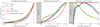 |
Fig. 3 Normalised S/N as a function of spectral resolution for different contributions as calculated with Eq. (8). From left to right are the speckle noise, photon noise, and detector noise limited regimes. A high-pass filter was appliedto move from the speckle-limited regime to the photon and detector-limited regime. A planet with an effective temperature of 1200K and no rotational broadening is shown here. |
3.2 Spectral bandwidth
For a fixed detector size, plate scale, and FOV, there are a fixed number of available spectral bim per spaxel. Thus, this raises the question as to whether it is better to increase the spectral resolution or the spectral bandwidth. Here, we assumed that we are increasing the bandwidth wtithin the absorption features of the targeted species and thus that we capture more lines. While this assumption is only valid for CO over a small wavelength range, it is more reasonable for water, which is the dominant contributor to the spectra of the planets specified in Table 1. The assumption and the wavelength range in which different molecule have absorption features is discussed in Sect. 3.3. In this simplified case, it can be seen from Eq. (8) that:
 (11)
(11)
Since the product of B × R needs to be constant to not increase the number of required pixels it is thus preferable to increase the spectral resolution if the increase in the S/N is steeper than  . Following our calculations from Sect. 3.1 and assuming that the globally calculated power spectrum is applicable locally, we were able to calculate this trade-off. The result for a planet with an effective temperature of ~ 1200 K in the photon-limited regime is shown in Fig. 4, assuming there is a total of 200 spectral bins per spaxel. We ended up with the same S/N curve as in the detector-limited regime from Fig. 3. If the spectrum consists of δ-lines, it does not matter whether we increase the spectral resolution or the bandwidth, as the S/N is proportional to
  . However, for water and a BT-SETTL spectrum, we found that it is best to increase the spectral resolution until ~2000 and after that to first maximise the bandwidth. If the goal is to detect the presence of methane or carbon monoxide, the optimum spectral resolution is even lower. However, since these molecules have very specific wavelength ranges in which they have absorption features, as is shown in Sect. 3.3, it is usually not beneficial to increase the bandwidth beyond these absorption bands.
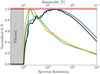 |
Fig. 4 Trade-off between spectral resolution and bandwidth showing the normalised S/N in the case where the total number of spectral bins is constant. Planet models with an effective temperature of 1200 K were used. |
3.3 Central wavelength
In the previous section we assumed that the molecular absorption features are evenly distributed across the wavelength range and the noise is constant. However, this is not realistic, and we have to choose the optimal wavelength range for the instrument. We considered ground-based observations and focussed on the J, H, and K bands in the near-infrared. In these bands, the spectra of warm gas giants exhibit significant molecular absorption, while she sky background remains manageable. These are also the bands that are predominansly used in current high-contrast imaging instruments. There are multiple effetcts that impact the S/N that can be achieved as a function of wavelength. Firstly, the emitted flux of the planet is wavelength dependent, and molecular absorption bands are present at specific wavelength ranges. Secondly, a higher Strehl ratio, and more starlight suppression, can be achieved at longer wavelengths. On the other hand, the separation between the star and planet is less λ/D at these longer wavelengths, which could mean worse performance of the coronagraph. Finally, the sky background starts to increase in the K-band.
Our framework presented in Sect. 2 considers all these effects. We used the simulated datacubes for the mock obsevation settings described in Sect. 2.3 and the three systems from Table 1. We calculated the matched filter S/N for a 3% bandwidth around each wavelength bin using Eq. (1), assuming a spectral resolution of 5000. This was done for four different templates, a BT-SETTL model of the appropriate effective temperature and the three most prominent molecular absorbers in this wavelength range, namely, H2O, CO, and CH4. The results are shown in Fig. 5. We observed that T-type companions, such as 51 Eri b, are best detectable in the J-band and are dominated by water and methane absorption. On the other hand, L-type companions, such as β Pic b, are best observed in the K-band, with features of both CO and water. The H-band is well suited to detect both types of planets and has mainly water features and some methane for cooler planets. Planets with effective temperatures between these two have dominant spectral features in all three bands. We note that the highest S/N can often be achieved at the edges of the bands, especially for water. For example, there is a sharp feature at the end of the J-band, which is due to the start of the 1.4 µm water absorption band. Going to higher spectral resolutions may allow us to observe more efficiently at the edges of the bands, especially if there is a significant Doppler shift between the target and the Earth. When looking back at the assumption in Sect. 3.2, we observed that features are not evenly distributed across the wavelength range, especially for cooler planets and when targeting CO and CH4. This will shift the optimum of the trade-off to higher spectral resolutions and a smaller bandwidth. The amount by which this is shifted is strongly dependent on the number of available spectral bins and the central wavelength.
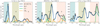 |
Fig. 5 Matched filter S/N between a BT-SETTL spectral model and molecular templates as a function of wavelength, assuming a 3% spectral bandwidth, a spectral resolution of 5000, and photon-limited observations. This is shown for three typical systems (from left to right): 51 Eri b, HR8799 e, and β Pic b. |
3.4 Field of view
Detecting planets usmg molecule mapping is most beneficial in the speckle-limited regime. This is because the high-pass filter is very effective at removing stellar speckles while leaving the high-order features in the planet spectrum intact. However, it generally results in the loss of the planet continuum. Farther away from the star, the gain in contrast from the speckle removal might be smaller than the loss of contrast from the removal of the planes continuum. In such cases, classical speckle removal post-processing techniques that keep the continuum (e.g. ADI) are expected to perform better. This limite the required FOV where molecule mapping is useful for increasing the detection capabilities of the instrument. The point at which tins occurs depends on many different factors. To illiustrate this, we considered an instrument with a 2k × 2k detector and considered the mock observations as described in Sect. 2.3. We assume that our instrument effectively uses 10% of the detector because of the placement of the spectra on the detector and is Nyquist sampled in the spatial and spectral dimensions. By increasing the FOV, we have fewer available detector pixels per spaxel. For example, for a FOV of 1.0″ in diameter in the H-band, there about 800 pixels spaxel−1, while for an FOV of 0.5″, there are about 320 pixels spaxel−1. This means we can increase the spectral resolution or bandwidth by decreasing the FOV, improving the gain that can be achieved with molecule mapping. We constructed contrast curves by considering ten different position angles for the planet at each separation and calculating the S/N according to Eq. (1). If the planet is detected at an S/N higher than five, it is considered detected. If not, the contrast between the planet and the star is decreased, and the process is repeated. The resulting contrast curves for different FOVs, spectral resolutions and bandwidshs are shown in Figs. 6 and 7. For simplicity, the wavelength coverage is centred at the mean wavelength of each band. We observed that a deeper contrast can be obtained for 51 Eri b than β Pic b, which is because cooler planets generally Cave more spectral features with respect to the continuum. We also saw that a higher spectral resolution inaeases the achievable contrast, at the cost of a smaller discovery space.
As we wanted to compare the obtatned contrast curves to the performance of the ADI, we divided up the available data of the reconstructed XAO residuals into ten sequential sete and simulated the resulting broadband images. A model of the PSF was then obtained by taking the median of these images. This model was subsequently subtracted from all the individual images, which were summed to obtain the residual image. The residual speckle noise was then estimated by radially computing the standard deviation. We then corrected for the ADI throughput using injection and recovery, assuming a total field rotation of 40°. This was a simplified simulation of the ADI performance, and it is likely overestimated, as we did not consider evolving the NCPA, for example. Still, it demonstrates the point that at a certain separation, the loss of continuum in molecule mapping degrades the achievable contrast, unlike ADI, which retains the continuum. These simulations show that in this specific case, it is not beneficial to go beyond a separation of ~0.5″ for the simulated 51 Eri b observations and beyond ~0.3″ for the simulated β Pic b observations. An important note is that for molecule mapping, assuming negligible detector noise, we have S/N ∝  , and we can thus increase the contrast by integrating longer. On the other hand, this is not necessarily the case for ADI, as we may be limited by quasi-static speckles that do not average over time (Vigan et al. 2022). On the other hand, ADI is less affected by phenomenon that dampen spectral features, such as clouds in the exoplanet’s atmosphere (Mollière et al. 2020) or dust extinction (Cugno et al. 2021). Finally, we note that both methods are not mutually exclusive, as a spectral matched filter can in principle s-ill be applied after using ADI for speckle removal.
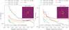 |
Fig. 6 Contrast curves with molecule mapping from the simulated observations. Different lines are for different combinations of spectral resolution and FOVs, and all use the same number of detector pixels. The inset shows the residuals after applying ADI on the mock observations. Left: 51 Eri b in the J-band with a 5% spectral bandwidth. Right: β Pic b in the H-band with a 10% bandwidth. |
4 Validation on VLT/SINFONI data
The concluions from she previous sections were based on analytical arguments or idealised end-to-end simulations. However, real observations have more complexity. For example, correlated noise may be present, which may be more prominent at certain spectral resolutions. While there is currently not an IFS with a spectral resolution greater than 1000 behind a high-contrast imaging system, molecule mapping has been used to successfully detect molecules in β Pic b and the HR8799 planets using VLT/SINFONI ond Keck/OSIRIS, respectively (Hoeijmakers et al. 2018; Ruffio et al. 2021), even though they lack the stellar suppression that can be achieved through XAO and coronagraphy. To validate our found trade-offs, we made use of archival VLT/SINFONI data of β Pic b taken on 10 September 2014 originally published in Hoeijmakers et al. (2018).
4.1 Data and analysis
The SINFONI dataset consisted of 24 science frames of the β Pictoris system with exposure times of 60 seconds in four dithering positions. Each spaxel in the datacube covered 0.0125″ by 0.025″, and the spectra had a spectral resolution of ~4500. The star was placed outside the FOV in these observations to allow for longer exposures. Furthermore, they were taken in pupil tracking mode to facilitate the application of ADI. We followed the data reduction process of Hoeijmakers et al. (2018). First, a master spectrum was generated from the 20 brightest spaxels. To obtain a model of the modulation of the stellar spectrum at each spaxel, we divided the signal in each spaxel by this master spectrum and subsequently low-pass filtered it by convolving with a Gaussian kernel with a standard deviation of 0.01 µm. This modulation was then multiplied with the master spectrum again and was subtracted from each spaxel. This method does not consider line spread dunction variations across the FOV. Furthermore, if the planet is really close to the star, spectral features of the planet may leak into the master spectrum, leading to self-subtraction. To remove correlated high-order structures, we did a PCA on the spectra of all spaxels and subtracted the first few fitted PCA modes. After this, we used Eq. (1) to calculate the matched filter S/N for three different high-pass filtered templates: a BT-SETTL model with Teff = 1700 K and log(g) = 4.0 and templates of the contribution of H2O and CO. We again used a Gaussian for the spatial part of the matched filter, with the standard deviation obtained from fitting the stellar PSF. Unlike in the simulafions, we did not know the uncertainty of each data point. The uncertainty of each wavelength bin was estimated by taking the standard deviation over all the spaxels. Afier the matched filter, we empirically normalised the detection map by calculating the mean and standard deviation of all the spaxels within a radius of 15 pixels of the planet while excluding a radius of 7 pixels around the centre oh the planet signal. The mean was then subtracted, and we divided by the standard deviation. While this allowed for an estimate of the S/N, the accurate estimation of the true detection significance in real observations remained complex.
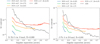 |
Fig. 7 S ame as Fig. 6 but the spectral resolution is fixed at R = 8000 while varying the spectral bandwidth. |
4.2 Spectral resolution
In Sect. 3.1, we studied the effect of the spectral resolution under idealised circumstances, that is, where the stellar and telluric contributions are perfectly removed. However, a higher spectral resolution may improve our ability to remove these contributions. We therefore studied the effect of spectral resolution on real observations. Before applying the data analysis described in Sect. 4.1, we degraded the cubes to different spectral resolutions. This was done by convolving with a Gaussian kernel with an FWHM corresponding to that spectral resolution and then down-sampling the spectrum for each spaxel. Molecule mapping was then applied to each of these datasets. Since we had a different number of data points for each spectral resolution, the optimal number of PCA components to apply would potentially also be different. Therefore, we subtracted one, three, five, eight and ten modes and chose the one that gave the highest detection S/N. The resulting detection maps for different spectral resolutions and the three templates are shown in Fig. 8. This figure shows that even if the spectral resolution of the instrument would have been ~300, we would have had very strong detections of both water and CO.
Figure 9 shows the peak detection S/N as a function of spectral resolution. The results are similar to the ones obtained in Sect. 3.1.4, even though the S/N estimation here may be less accurate. The figure again shows that CO can be detected at lower spectral resolutions than water. We also note that the S/N does not increase after R ~ 2000 and even decreases for the BT-SETTL model. This could be the result of an imperfect wavelength solution for each of the exposures, effectively decreasing the true spectral resolution of the observations. Alternatively, it could be due to inaccuracies in tie used line lists, which is more important at higher spectral resolutions.
4.3 Spectral resolution versus bandwidth
We also validated the results from the spectral resolution versus bandwidth trade-off obtained in Sect. 3.2. We again degraded the spectra of all spaxels to different spectral resolutions but adjusted the bandwidth such that the total number of spectral bins remained constant. We used a total of 100 spectral bins per spaxel. We did the S/N calculation for ten different central wavelengths linearly separated between 2.32 and 2.38 µm and took the mean. This wavelength range ensured that we had contributions from both water and CO. The results of this trade-off are shown in Fig. 10. We observed that the peak S/N for CO is obtained around R ~ 600, while for water it is around R ~ 1000. The curve for the water signal is in good agreement with what we found in Sect. 3.2. For CO, we found a slightly higher optimal spectral resolution. This is the result of the CO features not being distributed over the entire wavelength range such that we did not gain anything from increasing the spectral coverage beyond a certain point. Furthermore, at R ~ 100 we may still be in the speckle-limited regime. In this case, the BT-SETTL S/N also peaked at the same spectral resolution as CO. The reason for this is that CO is a more dominant contributor to the spectrum for hotter planets in the K-band than water, as was found in Sect. 3.3. In contrast, the spectrum studied in Sect. 3.2 was dominated by water features.
5 Atmospheric characterisation
Next to improving the detection limits of the instrument, an IFS immediately provides a spectrum of the planet which can be used to characterise its atmosphere. A common approach to infer properties about exoplanet atmospheres is through retrievals. The retrievals use a forward model and a sampler to obtain the posterior distributions of the parameters given the observed spectrum. This approach has successfully been applied for low-, medium-, and high-resolution spectra of a directly imaged planet in order to infer its ptmospheric propeaties (e.g. Samland et al. 2017; Mollière et al. 2020; Zhang et al. 2021; Wang et al. 2021). Assuming a Gaussian likelihood function ℒ, we have:
 (12)
(12)
The latter term is the same as in Eq. (1), which gives the S/N of a matched filter. The relation between likelihood and cross-correlation is discussed in more detail in Brogi & Line (2019) and Ruffio et al. (2019).
When inferring pronerties of exoplanet atmospheres, the absolute value of the likelihood is not of interest Instead, the difference in likelehoods between two models is of interest with parameters θ and θ + Δθ:
 (13)
(13)
The obtained constraints on the parameters thus depends on how much the template chahges as a function of the targeted parameter. It is not straightforward to derive this analytically as a function of, for example, spectral resolution. Instead, the effect of the spectral resolution on the obtamed confidence inservals of different parnmeters is numerically studied. We setup a retrieval framework using petitRADTRANS (Mollière et al. 2019) and emcee (Foreman-Mackey et al. 2013). We used the following free parameters in our forward model: C/O ratio, metallicity, log(g), a flux scaling factor determined by the radius of the planet and distance, the radial velocity of the planet, and its spin along the line of sight υsin(i). Finally, we parameterised the pressure-temperature (P–T) profile of the planet using four free points logarithmically distributed between 0.02 bar and 5 bar. We did not allow for temperature inversions and obtained the full P–T profile using cubic spline interpolation from the four points. We used the mock observations of HR8799 e in the H-band from Sect. 2.3. Since the data analysis generally results in the loss of the planet continuum, we retrieved the continuum-removed planetary spectrum. We ran a chain of 100 walkers for 3000 steps and subsequently calculated the 68% confidence interval for the last 1000 steps. The obtained 68% confidence intervals for the different parameters are shown in Fig. 11 and an example corner plot of the obtained posteriors is shown in Appendix E. The constraint on the temperature profile is the averaged uncertainty interval on the four temperature points. For comparison, we over-plotted the confidence intervals with a scaled and fitted version of the inverse matched filter S/N. If the S/N of the planet detection increased, this led to an increase in the maximum likelihood, and we thus expected the confidence interval to shrink.
We observed that for the C/O ratio, metallicity, surface gravity, and the temperature profile, the dependency on spectral resolution followed that of the matched filter S/N. We therefore argue that trade-offs from the previous sections also hold for the constraints on these parameters. As expected, different behaviour was found for the radial velocity and spin of the planet. For the radial velocity, we saw an (R × S/N)−1 dependence as a result of the smaller resolution element and increase in S/N. The constraint on the spin of the planet was more complex. At a low spectral resolution, this constraint is just an upper limit, as we do not resolve the lines themselves. From R ~ 8000, the line shape starts to be dominated by the rotational broadening, as opposed to the instrumental profile, leading to a sudden decrease in the uncertainty on υsini. An important caveat is that we did not include clouds in these retrievals, which are known to lead to degeneracies at a lower spectral resolution. A more thorough analysis of the model degeneracies and parameter information content (Line et al. 2012; Batalha & Line 2017) at different spectral resolutions and instrument configurations will be the subject of future work.
 |
Fig. 8 Detection maps of the β Pictoris SINFONI data. Each column shows the detection map at a different spectral resolution, while the rows are for different cross-correlation templates. |
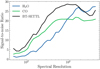 |
Fig. 9 Detection S/N of β Pictoris b in the SINFONI data as a function of the spectral resolution to which all datacubes are convolved for H2O, CO, and BT-SETTL templates. |
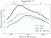 |
Fig. 10 Detection S/N of β Pic b in the SINFONI data in the case where the number of spectral bins is fixed. A higher spectral resolution there-fore means a lower spectral bandwidth. |
6 Conclusions
We have studied the trade-offs between the spectral resolution, spectral bandwidth, and FOV for the detection and characterisation capabilities of an IFS behind a high-contrast imaging system. This was studied through end-to-end simulations, analytical considerations, and atmospheric retrievals. The results were then verified on archival data of β Pic b with VLT/SINFONI. While we have mainly considered the molecule mapping framework from Hoeijmakers et al. (2018), our results should be independent of the exact analysis framework (e.g. Ruffio et al. (2019)), except for the results on the SINFONI data. The main conclusions from this work are the following:
Molecular absorption spectra have decreasing power for higher spectral resolution. Moderate spectral resolutions (R ≳ 300) are therefore already powerful for boosting detection limits with molecule mapping;
In order to get the highest S/N, it is best to increase the spectral resolution until R ~ 2000 and then maximise the wavelength coverage of the instrument or observations within the observing band;
Molecule mapping is most beneficial in the speckle-limited regime close to the star. Further away, the loss of the planet continuum results in classical approaches potentially giving similar or better performance. Therefore, such instruments do not need to have a large FOV;
T-type companions are best detectable in the J/H band through water and methane features, while L-type companions are best detectable in the K/H band through CO and water features. The highest detection S/N can often be achieved at the edges of the observing bands;
Constraints on atmospheric parameters such as the C/O ratio, metallicity, surface gravity, and the temperature profile, follow similar trade-offs as detection. Higher spectral resolution is needed to obtain constraints on the radial velocity and spin of the planet.
Our results can help guide decisions about instrument designs or observing plans for current and future high-contrast integral field spectrographs in the near-infrared, such as VLT/SPHERE+ZMedRes, ELT/HARMONI, or ELT/PCS. Future work will investigate how these trade-offs change when searching for planets in reflected light.
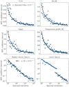 |
Fig. 11 Constraints on the free parameters from the retrievals as a function of spectral resolution. Also shown is the inverse matched filter S/N for the top two rows and a (R × S/N)−1 relation for the bottom row. |
Acknowledgements
We thank Arthur Vigan for providing us the representative XAO residuals for SPHERE. We also want to thank the referee for suggestions that have resulted in major improvements in this work. R.L. and LS. acknowledge funding from the European Research Council (ERC) under the European Union’s Horizon 2020 research and innovation program under grant agreement No 694513. This work has been supported by a grant from Labex OSUG (Investissements d’avenir – ANR10 LABX56). C.D. is part of Labex OSUG (ANR10 LABX56), and C.D. acknowledges support from the European Research Council under the European Union’s Horizon 2020 research and innovation program under grant agreement no. 832428-Origins.
Appendix A Spectral models and templates
The spectral models and templates used throughout this work are shown in Fig. A.1 for a spectral resolution of 30,000.
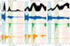 |
Fig. A.1 Flux density of the spectral models and templates used throughout this study shown at a spectral resolution of 30,000. The molecular templates have been high-pass filtered. |
Appendix B Power spectral densities for different planets
Fig B.1 shows the PSDs of β Pic b-like and 51 Eri b-like planets.
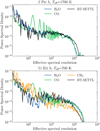 |
Fig. B.1 Power spectral densities of the planetary and molecular templates for a β Pic b-like (top) and 51 Eri b-like (bottom) planets. |
Appendix C Derivation of the relation between the cross-correlation S/N and the power spectral density
Given a spectrum si, template ti, and Gaussian noise with standard deviation σi, the S/N of a matched filter is given by (Ruffio et al. 2017):
 (C.1)
(C.1)
where N is the number of data points indexed by i. For simplicity in these derivations, we assumed that the planet signal is concentrated in a single spaxel with M spectral bins. Assuming we have a perfect model (si = ti + n) and uncorrelated noise that is roughly constant for each datapoint (σi ≈ σ), we have:
 (C.2)
(C.2)
In the case that ti is sampled at a sufficient rate such that we can reconstruct the continuous signal t, (i.e. we Nyquist sample the spectrum), we have  , with < t2 > denoting the average value of t2. This gives:
 (C.3)
(C.3)
We defined the wavelength sampling such that we have constant spectral resolution across the entire wavelength range (i.e. (λi+1 – λi)/λi = constant). We did this by defining a wavelength grid uniformly in log λ. We can use the Wiener-Khinchin theorem to express this in terms of the PSD:
![$ lt; {t^2}\left( {\log \lambda } \right) > = {R_t}\left( 0 \right) = \int_{ - \infty }^\infty {{\rm{PSD}}\left[ {t\left( {\log \lambda } \right)} \right]} \left( f \right)d\,f.$](/articles/aa/full_html/2023/07/aa45169-22/aa45169-22-eq33.png) (C.4)
(C.4)
Here, Rt is the autocorrelation function of t(log λ), PSD[t(log λ)] is the PSD of t(log λ) as defined in Eq. 4, and f = 1/(Δ log λ′) is the frequency of the corresponding fluctuation. One can also express the PSD in terms of an effective spectral resolution R′ by using:
 (C.5)
(C.5)
The factor of two comes from the fact that we needed to Nyquist sample the spectrum to see fluctuations of a specific frequency. This means that we have R′ = f /2, df = 2dR′, and that log λ and 2R′ are Fourier conjugate variables. Furthermore, we can use that t is real-valued to turn Eq. C.4 into a one-sided integral with an additional factor of two. Together this gives:
![$ < {t^2} > = 4\int_0^\infty {{\rm{PSD}}\left[ t \right]\left( {R'} \right)dR'} $](/articles/aa/full_html/2023/07/aa45169-22/aa45169-22-eq35.png) (C.6)
(C.6)
The noiseless observed spectrum t consists of the planet spectrum tp convolved with the line spread function lsfR of the instrument, the detector sampling function sR, and a filter describing the effect of the data cleaning c (e.g. the high-pass filter):
 (C.7)
(C.7)
These convolutions become multiplications in Fourier space:
 (C.8)
(C.8)

where H(R′) = LSFR(R′)SR(R′)C(R′) is the combined transfer function of the spectrograph and data reduction. We then have:
 (C.10)
where P(R′) = PSD[tp] is the PSD of the planet spectrum as defined in Eq. 4. Substituting this into Eq. C.3, we obtain:
 (C.11)
In the Nyquist-sampled case, we have M = 2BR, with B = (λmax – λmin)/λcentral the spectral bandwidth, giving:
 (C.12)
Next, we describe some simplifying assumptions we made on the filter H(R′). We first assumed that we have an idealised spectrograph where the line spread and sampling function together as an ideal low-pass filter, removing all fluctuations with frequencies higher than R:
 (C.13)
Here, the 1/R is to make sure that the line spread function is normalised and the flux is conserved. Finally, we assumed that the data reduction is an ideal high-pass filter that removes all features below R′ = Rmin. This then simplifies Eq. (C.12) to:
 (C.14)
Appendix D Numerical validation of the matched filter S/N equation
Here we show a numerical validation of the equation derived in Appendix C. We used the mock observations of HR8799e in the H-band as described in Section 2.3 as a test case. We calculated the cross-correlation S/N in three ways: 1) The first method was by applying Eq. 1 on the full simulated datacube. This is the baseline and most accurate case, as it includes the most effects. In the speckle-noise limited case this equation is not applicable, and we calculated the S/N by normalizing by the standard deviation of the cross-correlation function away from the peak (as in e.g. Hoeijmakers et al. (2018); Snellen et al. (2014)). 2) The second approach used Eq. 8 based on the PSD, which assumes wavelength independent errors. For this method, we used Gaussians for LSF(R′) and C(R′) with appropriate standard deviations, given the spectral resolution and high-pass filter applied to the data. 3) The third method used Eq. 9, which makes further simplifying assumptions on the properties of the spectrograph and data reduction. The resulting S/N curves of the methods are shown in Fig. D.1. It shows good agreement between the three equations, except at very low and very high spectral resolutions, where some of the assumptions break down.
 |
Fig. D.1 Numerical validation of the relation between the PSD and the S/N of the matched filter. |
Appendix E Example retrieval result
An example corner plot from the retrieval study for HR8799e with a spectral resolution of 1,000 in the H-band is shown in Fig. E.1. The free parameters are the metallicity [Fe/H], C/O ratio, surface gravity log(g), scaling parameter a, rotational velocity vsini, temperature nods T1 through T4, and the radial velocity (RV).
 |
Fig. E.1 Example corner plot for a retrieval of HR8799e in the H-band with a spectral resolution of 1,000. |
References
- Allard, F. 2014, in Exploring the Formation and Evolution of Planetary Systems, 299, eds. M. Booth, B. C. Matthews, & J. R. Graham, 271 [NASA ADS] [Google Scholar]
- Barman, T. S., Konopacky, Q. M., Macintosh, B., & Marois, C. 2015, ApJ, 804, 61 [Google Scholar]
- Batalha, N. E., & Line, M. R. 2017, AJ, 153, 151 [NASA ADS] [CrossRef] [Google Scholar]
- Beuzit, J. L., Vigan, A., Mouillet, D., et al. 2019, A&A, 631, A155 [NASA ADS] [CrossRef] [EDP Sciences] [Google Scholar]
- Birkby, J. L., de Kok, R. J., Brogi, M., et al. 2013, MNRAS, 436, L35 [Google Scholar]
- Boccaletti, A., Chauvin, G., Mouillet, D., et al. 2020, arXiv e-prints, [arXiv:2003.05714] [Google Scholar]
- Bohn, A. J., Kenworthy, M. A., Ginski, C., et al. 2020, MNRAS, 492, 431 [Google Scholar]
- Bohn, A. J., Ginski, C., Kenworthy, M. A., et al. 2021, A&A, 648, A73 [NASA ADS] [CrossRef] [EDP Sciences] [Google Scholar]
- Bonnefoy, M., Boccaletti, A., Lagrange, A. M., et al. 2013, A&A, 555, A107 [NASA ADS] [CrossRef] [EDP Sciences] [Google Scholar]
- Bowler, B. P. 2016, PASP, 128, 102001 [Google Scholar]
- Brandl, B., Bettonvil, F., van Boekel, R., et al. 2021, The Messenger, 182, 22 [NASA ADS] [Google Scholar]
- Brogi, M., & Line, M. R. 2019, AJ, 157, 114 [Google Scholar]
- Brogi, M., Snellen, I. A. G., de Kok, R. J., et al. 2012, Nature, 486, 502 [Google Scholar]
- Brogi, M., de Kok, R. J., Birkby, J. L., Schwarz, H., & Snellen, I. A. G. 2014, A&A, 565, A124 [NASA ADS] [CrossRef] [EDP Sciences] [Google Scholar]
- Bryan, M. L., Benneke, B., Knutson, H. A., Batygin, K., & Bowler, B. P. 2018, Nat. Astron., 2, 138 [Google Scholar]
- Carlomagno, B., Delacroix, C., Absil, O., et al. 2020, J. Astron. Telescopes Instrum. Syst., 6, 035005 [Google Scholar]
- Chauvin, G., Desidera, S., Lagrange, A. M., et al. 2017, A&A, 605, A9 [EDP Sciences] [Google Scholar]
- Cheetham, A., Bonnefoy, M., Desidera, S., et al. 2018, A&A, 615, A160 [NASA ADS] [CrossRef] [EDP Sciences] [Google Scholar]
- Cugno, G., Patapis, P., Stolker, T., et al. 2021, A&A, 653, A12 [NASA ADS] [CrossRef] [EDP Sciences] [Google Scholar]
- Currie, T., Brandt, T. D., Kuzuhara, M., et al. 2020, ApJ, 904, L25 [Google Scholar]
- Currie, T., Lawson, K., Schneider, G., et al. 2022, Nat. Astron., 6, 751 [NASA ADS] [CrossRef] [Google Scholar]
- Davies, R., Esposito, S., Schmid, H. M., et al. 2018, SPIE Conf. Ser., 10702, 1070209 [Google Scholar]
- de Kok, R. J., Brogi, M., Snellen, I. A. G., et al. 2013, A&A, 554, A82 [NASA ADS] [CrossRef] [EDP Sciences] [Google Scholar]
- Delorme, J.-R., Jovanovic, N., Echeverri, D., et al. 2021, J. Astron. Telescopes Instrum. Syst., 7, 035006 [NASA ADS] [Google Scholar]
- Echeverri, D., Ruane, G., Calvin, B., et al. 2020, SPIE Conf. Ser., 11446, 1144619 [NASA ADS] [Google Scholar]
- Eriksson, S. C., Asensio Torres, R., Janson, M., et al. 2020, A&A, 638, A6 [Google Scholar]
- Foreman-Mackey, D., Hogg, D. W., Lang, D., & Goodman, J. 2013, PASP, 125, 306 [Google Scholar]
- Gratton, R., Keller, C., Diolaiti, E., et al. 2022, in Ground-based and Airborne Instrumentation for Astronomy IX, (SPIE), 121844F [Google Scholar]
- GRAVITY Collaboration (Lacour, S., et al.) 2019, A&A, 623, A11 [NASA ADS] [CrossRef] [EDP Sciences] [Google Scholar]
- Haffert, S. Y., Bohn, A. J., de Boer, J., et al. 2019, Nat. Astron., 3, 749 [Google Scholar]
- Haffert, S. Y., Harris, R. J., Zanutta, A., et al. 2020, J. Astron. Telescopes Instrum. Syst., 6, 045007 [NASA ADS] [Google Scholar]
- Hoeijmakers, H. J., Schwarz, H., Snellen, I. A. G., et al. 2018, A&A, 617, A144 [NASA ADS] [CrossRef] [EDP Sciences] [Google Scholar]
- Houllé, M., Vigan, A., Carlotti, A., et al. 2021, A&A, 652, A67 [NASA ADS] [CrossRef] [EDP Sciences] [Google Scholar]
- Husser, T. O., Wende-von Berg, S., Dreizler, S., et al. 2013, A&A, 553, A6 [NASA ADS] [CrossRef] [EDP Sciences] [Google Scholar]
- Jovanovic, N., Martinache, F., Guyon, O., et al. 2015, PASP, 127, 890 [NASA ADS] [CrossRef] [Google Scholar]
- Jovanovic, N., Guyon, O., Kotani, T., et al. 2017, arXiv e-prints, [arXiv:1712.07762] [Google Scholar]
- Jovanovic, N., Delorme, J. R., Bond, C. Z., et al. 2019, arXiv e-prints, [arXiv:1909.04541] [Google Scholar]
- Kasper, M., Cerpa Urra, N., Pathak, P., et al. 2021, The Messenger, 182, 38 [Google Scholar]
- Keppler, M., Benisty, M., Müller, A., et al. 2018, A&A, 617, A44 [NASA ADS] [CrossRef] [EDP Sciences] [Google Scholar]
- Konopacky, Q. M., Barman, T. S., Macintosh, B. A., & Marois, C. 2013, Science, 339, 1398 [Google Scholar]
- Konopacky, Q. M., Rameau, J., Duchêne, G., et al. 2016, ApJ, 829, L4 [Google Scholar]
- Kotani, T., Kawahara, H., Ishizuka, M., et al. 2020, SPIE Conf. Ser., 11448, 1144878 [NASA ADS] [Google Scholar]
- Lagrange, A. M., Bonnefoy, M., Chauvin, G., et al. 2010, Science, 329, 57 [Google Scholar]
- Line, M. R., Zhang, X., Vasisht, G., et al. 2012, ApJ, 749, 93 [Google Scholar]
- Macintosh, B., Graham, J. R., Ingraham, P., et al. 2014, PNAS, 111, 12661 [NASA ADS] [CrossRef] [Google Scholar]
- Macintosh, B., Graham, J. R., Barman, T., et al. 2015, Science, 350, 64 [Google Scholar]
- Marois, C., Lafrenière, D., Doyon, R., Macintosh, B., & Nadeau, D. 2006, ApJ, 641, 556 [Google Scholar]
- Marois, C., Zuckerman, B., Konopacky, Q. M., Macintosh, B., & Barman, T. 2010, Nature, 468, 1080 [NASA ADS] [CrossRef] [Google Scholar]
- Martinez, P., Dorrer, C., Kasper, M., Boccaletti, A., & Dohlen, K. 2009, A&A, 500, 1281 [NASA ADS] [CrossRef] [EDP Sciences] [Google Scholar]
- Milli, J., Hibon, P., Christiaens, V., et al. 2017, A&A, 597, A2 [Google Scholar]
- Mollière, P., Wardenier, J. P., van Boekel, R., et al. 2019, A&A, 627, A67 [Google Scholar]
- Mollière, P., Stolker, T., Lacour, S., et al. 2020, A&A, 640, A131 [Google Scholar]
- Mollière, P., Molyarova, T., Bitsch, B., et al. 2022, ApJ, 934, 74 [CrossRef] [Google Scholar]
- N’Diaye, M., Soummer, R., Pueyo, L., et al. 2016, ApJ, 818, 163 [Google Scholar]
- Nielsen, E. L., De Rosa, R. J., Macintosh, B., et al. 2019, AJ, 158, 13 [Google Scholar]
- Noll, S., Kausch, W., Barden, M., et al. 2012, A&A, 543, A92 [NASA ADS] [CrossRef] [EDP Sciences] [Google Scholar]
- Otten, G. P. P. L., Vigan, A., Muslimov, E., et al. 2021, A&A, 646, A150 [EDP Sciences] [Google Scholar]
- Patapis, P., Nasedkin, E., Cugno, G., et al. 2022, A&A, 658, A72 [NASA ADS] [CrossRef] [EDP Sciences] [Google Scholar]
- Petit dit de la Roche, D. J. M., Hoeijmakers, H. J., & Snellen, I. A. G. 2018, A&A, 616, A146 [EDP Sciences] [Google Scholar]
- Petrus, S., Bonnefoy, M., Chauvin, G., et al. 2021, A&A, 648, A59 [EDP Sciences] [Google Scholar]
- Por, E. H., Haffert, S. Y., Radhakrishnan, V. M., et al. 2018, SPIE Conf. Ser., 10703, 1070342 [NASA ADS] [Google Scholar]
- Rajan, A., Rameau, J., De Rosa, R. J., et al. 2017, AJ, 154, 10 [Google Scholar]
- Rameau, J., Chauvin, G., Lagrange, A. M., et al. 2015, A&A, 581, A80 [NASA ADS] [CrossRef] [EDP Sciences] [Google Scholar]
- Riaud, P., & Schneider, J. 2007, A&A, 469, 355 [NASA ADS] [CrossRef] [EDP Sciences] [Google Scholar]
- Ruffio, J.-B., Macintosh, B., Wang, J. J., et al. 2017, ApJ, 842, 14 [Google Scholar]
- Ruffio, J.-B., Macintosh, B., Konopacky, Q. M., et al. 2019, AJ, 158, 200 [Google Scholar]
- Ruffio, J.-B., Konopacky, Q. M., Barman, T., et al. 2021, AJ, 162, 290 [NASA ADS] [CrossRef] [Google Scholar]
- Samland, M., Mollière, P., Bonnefoy, M., et al. 2017, A&A, 603, A57 [NASA ADS] [CrossRef] [EDP Sciences] [Google Scholar]
- Schwarz, H., Ginski, C., de Kok, R. J., et al. 2016, A&A, 593, A74 [NASA ADS] [CrossRef] [EDP Sciences] [Google Scholar]
- Snellen, I. A. G., Brandl, B. R., de Kok, R. J., et al. 2014, Nature, 509, 63 [Google Scholar]
- Snellen, I., de Kok, R., Birkby, J. L., et al. 2015, A&A, 576, A59 [NASA ADS] [CrossRef] [EDP Sciences] [Google Scholar]
- Soummer, R. 2005, ApJ, 618, L161 [Google Scholar]
- Sparks, W. B., & Ford, H. C. 2002, ApJ, 578, 543 [Google Scholar]
- Thatte, N., Tecza, M., Schnetler, H., et al. 2021, The Messenger, 182, 7 [NASA ADS] [Google Scholar]
- Vigan, A., Otten, G. P. P. L., Muslimov, E., et al. 2018, SPIE Conf. Ser., 10702, 1070236 [NASA ADS] [Google Scholar]
- Vigan, A., N’Diaye, M., Dohlen, K., et al. 2019, A&A, 629, A11 [NASA ADS] [CrossRef] [EDP Sciences] [Google Scholar]
- Vigan, A., Fontanive, C., Meyer, M., et al. 2021, A&A, 651, A72 [EDP Sciences] [Google Scholar]
- Vigan, A., Dohlen, K., N’Diaye, M., et al. 2022, A&A, 660, A140 [NASA ADS] [CrossRef] [EDP Sciences] [Google Scholar]
- Wang, J., Mawet, D., Ruane, G., Hu, R., & Benneke, B. 2017, AJ, 153, 183 [Google Scholar]
- Wang, J. J., Ruffio, J.-B., Morris, E., et al. 2021, AJ, 162, 148 [NASA ADS] [CrossRef] [Google Scholar]
- Wilcomb, K. K., Konopacky, Q. M., Barman, T. S., et al. 2020, AJ, 160, 207 [Google Scholar]
- Xin, Y., Jovanovic, N., Ruane, G., et al. 2022, ApJ, 938, 140 [NASA ADS] [CrossRef] [Google Scholar]
- Zhang, Y., Snellen, I. A. G., Bohn, A. J., et al. 2021, Nature, 595, 370 [NASA ADS] [CrossRef] [Google Scholar]
All Tables
Assumed parameters of the planetary systems used for the simulations throughout this paper.
Summary of the relation between the S/N of a matched filter and the spectral resolution in the three different noise regimes with .
All Figures
|
Fig. 1 Visualisation of the simulated datacubes. Left: resulting wavelength summed H-band images from the simulations described in Sect. 2.1. Middle: same but including am implementation of the APLC. Right: example result of me data analysis. The location of the planet is indicated with a red circle. |
| In the text | |
|
Fig. 2 Normalised PSD of different contributions to the observed spectrum between 1 and 2.5 µm. Here, we assumed a planet with an effective temperature of 1200 K and log(g) of 4.0. The panels show the results without rotational broadening (top) and with rotational broadening of υrot sin i = 15 km s−1 (bottom). |
| In the text | |
|
Fig. 3 Normalised S/N as a function of spectral resolution for different contributions as calculated with Eq. (8). From left to right are the speckle noise, photon noise, and detector noise limited regimes. A high-pass filter was appliedto move from the speckle-limited regime to the photon and detector-limited regime. A planet with an effective temperature of 1200K and no rotational broadening is shown here. |
| In the text | |
|
Fig. 4 Trade-off between spectral resolution and bandwidth showing the normalised S/N in the case where the total number of spectral bins is constant. Planet models with an effective temperature of 1200 K were used. |
| In the text | |
|
Fig. 5 Matched filter S/N between a BT-SETTL spectral model and molecular templates as a function of wavelength, assuming a 3% spectral bandwidth, a spectral resolution of 5000, and photon-limited observations. This is shown for three typical systems (from left to right): 51 Eri b, HR8799 e, and β Pic b. |
| In the text | |
|
Fig. 6 Contrast curves with molecule mapping from the simulated observations. Different lines are for different combinations of spectral resolution and FOVs, and all use the same number of detector pixels. The inset shows the residuals after applying ADI on the mock observations. Left: 51 Eri b in the J-band with a 5% spectral bandwidth. Right: β Pic b in the H-band with a 10% bandwidth. |
| In the text | |
|
Fig. 7 S ame as Fig. 6 but the spectral resolution is fixed at R = 8000 while varying the spectral bandwidth. |
| In the text | |
|
Fig. 8 Detection maps of the β Pictoris SINFONI data. Each column shows the detection map at a different spectral resolution, while the rows are for different cross-correlation templates. |
| In the text | |
|
Fig. 9 Detection S/N of β Pictoris b in the SINFONI data as a function of the spectral resolution to which all datacubes are convolved for H2O, CO, and BT-SETTL templates. |
| In the text | |
|
Fig. 10 Detection S/N of β Pic b in the SINFONI data in the case where the number of spectral bins is fixed. A higher spectral resolution there-fore means a lower spectral bandwidth. |
| In the text | |
|
Fig. 11 Constraints on the free parameters from the retrievals as a function of spectral resolution. Also shown is the inverse matched filter S/N for the top two rows and a (R × S/N)−1 relation for the bottom row. |
| In the text | |
|
Fig. A.1 Flux density of the spectral models and templates used throughout this study shown at a spectral resolution of 30,000. The molecular templates have been high-pass filtered. |
| In the text | |
|
Fig. B.1 Power spectral densities of the planetary and molecular templates for a β Pic b-like (top) and 51 Eri b-like (bottom) planets. |
| In the text | |
|
Fig. D.1 Numerical validation of the relation between the PSD and the S/N of the matched filter. |
| In the text | |
|
Fig. E.1 Example corner plot for a retrieval of HR8799e in the H-band with a spectral resolution of 1,000. |
| In the text | |
Current usage metrics show cumulative count of Article Views (full-text article views including HTML views, PDF and ePub downloads, according to the available data) and Abstracts Views on Vision4Press platform.
Data correspond to usage on the plateform after 2015. The current usage metrics is available 48-96 hours after online publication and is updated daily on week days.
Initial download of the metrics may take a while.