| Issue |
A&A
Volume 690, October 2024
|
|
|---|---|---|
| Article Number | A125 | |
| Number of page(s) | 13 | |
| Section | Stellar atmospheres | |
| DOI | https://doi.org/10.1051/0004-6361/202450245 | |
| Published online | 01 October 2024 | |
Retrieving stellar parameters and dynamics of AGB stars with Gaia parallax measurements and CO5BOLD RHD simulations
1
Université Côte d’Azur, Observatoire de la Côte d’Azur, CNRS,
Lagrange,
CS 34229
Nice,
France
2
Theoretical Astrophysics, Department of Physics and Astronomy, Uppsala University,
Box 516,
751 20
Uppsala,
Sweden
3
Institute of Applied Physics, TU Wien,
Wiedner Hauptstraße 8-10,
1040
Vienna,
Austria
Received:
4
April
2024
Accepted:
16
July
2024
Context. The complex dynamics of asymptotic giant branch (AGB) stars and the resulting stellar winds have a significant impact on the measurements of stellar parameters and amplify their uncertainties. Three-dimensional (3D) radiative hydrodynamic (RHD) simulations of convection suggest that convection-related structures at the surface of AGB star affect the photocentre displacement and the parallax uncertainty measured by Gaia.
Aims. We explore the impact of the convection on the photocentre variability and aim to establish analytical laws between the photo-centre displacement and stellar parameters to retrieve such parameters from the parallax uncertainty.
Methods. We used a selection of 31 RHD simulations with CO5BOLD and the post-processing radiative transfer code OPTIM3D to compute intensity maps in the Gaia G band [320–1050 nm]. From these maps, we calculated the photocentre position and temporal fluctuations. We then compared the synthetic standard deviation to the parallax uncertainty of a sample of 53 Mira stars observed with Gaia.
Results. The simulations show a displacement of the photocentre across the surface ranging from 4 to 13% of the corresponding stellar radius, in agreement with previous studies. We provide an analytical law relating the pulsation period of the simulations and the photocentre displacement as well as the pulsation period and stellar parameters. By combining these laws, we retrieve the surface gravity, the effective temperature, and the radius for the stars in our sample.
Conclusions. Our analysis highlights an original procedure to retrieve stellar parameters by using both state-of-the-art 3D numerical simulations of AGB stellar convection and parallax observations of AGB stars. This will help us refine our understanding of these giants.
Key words: hydrodynamics / astrometry / parallaxes / stars: AGB and post-AGB / stars: atmospheres
© The Authors 2024
 Open Access article, published by EDP Sciences, under the terms of the Creative Commons Attribution License (https://creativecommons.org/licenses/by/4.0), which permits unrestricted use, distribution, and reproduction in any medium, provided the original work is properly cited.
This article is published in open access under the Subscribe to Open model. Subscribe to A&A to support open access publication.
1 Introduction
Low- to intermediate-mass stars (0.8–8 M⊙) evolve into the asymptotic giant branch (AGB), in which they undergo complex dynamics characterised by several processes including convection, pulsations, and shockwaves. These processes trigger strong stellar winds (10−8–10−5 M⊙/yr, De Beck et al. 2010) that significantly enrich the interstellar medium with various chemical elements (Höfner & Olofsson 2018). These processes and stellar winds also amplify uncertainties of stellar parameter determinations with spectro-photometric techniques, like the effective temperature, which in turn impacts the determination of mass-loss rates (Höfner & Olofsson 2018). In particular, Mira stars are peculiar AGB stars, showing extreme magnitude variability (larger than 2.5 mag in the visible) due to pulsations over periods of 100–1000 days (Decin 2021).
In Chiavassa et al. (2011, 2018, 2022), 3D radiative hydrodynamics (RHD) simulations of convection computed with CO5BOLD (Freytag et al. 2012; Freytag 2013, 2017) reveal the AGB photosphere morphology to be made of a few large-scale, long-lived convective cells and some short-lived and small-scale structures that cause temporal fluctuations on the emerging intensity in the Gaia G band [320–1050 nm]. The authors suggest that the temporal convective-related photocentre variability should substantially impact the photometric measurements of Gaia, and thus the parallax uncertainty. In this work, we use 31 recent simulations to establish analytical laws between the photocentre displacement and the pulsation period and then between the pulsation period and stellar parameters. We combine these laws and apply them to a sample of 53 Mira stars from Uttenthaler et al. (2019) to retrieve their effective stellar gravity, effective temperature, and radius thanks to their parallax uncertainty from Gaia Data Release 31 (GDR3) (Gaia Collaboration 2016, 2023).
2 Overview of the radiative hydrodynamics simulations
In this section, we present the simulations and the theoretical relations between the stellar parameters and the pulsation period. We also present how we compute the standard deviation of the photocentre displacement and its correlation with the pulsation period.
2.1 Methods
We used RHD simulations of AGB stars computed with the code CO5BOLD (Freytag et al. 2012; Freytag 2013, 2017). It solves the coupled non-linear equations of compressible hydrodynamics and non-local radiative energy transfer, assuming solar abundances, which is appropriate for M-type AGB stars. The configuration is ‘star-in-a-box’, which takes into account the dynamics of the outer convective envelope and the inner atmosphere. Convection and pulsations in the stellar interior trigger shocks in the outer atmosphere, giving a direct insight into the stellar stratification. Material can levitate towards layers where it can condensate into dust grains (Freytag & Höfner 2023). However, models used in this work do not include dust.
We then post-processed a set of temporal snapshots from the RHD simulations using the radiative transfer code OPTIM3D (Chiavassa et al. 2009), which takes into account the Doppler shifts, partly due to convection, in order to compute intensity maps integrated over the Gaia G band [320–1050 nm]. The radiative transfer is computed using pre-tabulated extinction coefficients from MARCS models (Gustafsson et al. 2008) and solar abundance tables (Asplund et al. 2009).
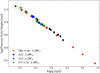 |
Fig. 1 Log-log plot of the surface gravity [cgs] versus the pressure scale height [cm]. As the effective temperature is near constant among all our models, we expect a linear relation. |
2.2 Characterising the AGB stellar grid
We used a selection of simulations from Freytag et al. (2017), Chiavassa et al. (2018) [abbreviation: F17+C18], Ahmad et al. (2023) [abbreviation: A23] and some new models [abbreviation: This work], in order to cover the 2000–10000 L⊙ range. The updated simulation parameters are reported in Table A.1.
In particular, 24 simulations have a stellar mass equal to 1.0 M⊙, and seven simulations have one equal to 1.5 M⊙. In the rest of this work, we denote by a 1.0 subscript the laws or the results obtained from the analysis of the 1.0 M⊙ simulations; and by a 1.5 subscript those obtained from the analysis of the 1.5 M⊙ simulations.
The pressure scale height is defined as  , with kB the Boltzmann constant, Teff the effective surface temperature, µ the mean molecular mass, and 𝑔 the local surface gravity. The lower the surface gravity is, the larger the pressure scale height becomes, and so the larger the convective cells can grow (see Fig. 1 and Freytag et al. 2017).
Moreover, Freytag et al. (1997) estimated that the characteristic granule size scales linearly with HP. Interplay between large-scale convection and radial pulsations results in the formation of giant and bright convective cells at the surface. The resulting intensity asymmetries directly cause temporal and spatial fluctuations of the photocentre. The larger the cells, the larger the photocentre displacement. This results in a linear relation between the photocentre displacement and the pressure scale height (Chiavassa et al. 2011, 2018). However, Chiavassa et al. (2011) found it is no longer true for Hp greater than 2.24 × 1010 cm for both interferometric observations of red super-giant stars and 3D simulations, suggesting that the relation for evolved stars is more complex and depends on Hp (Fig. 18 in the aforementioned article).
Concerning the pulsation period, Ahmad et al. (2023) performed a fast Fourier transform on spherically averaged mass flows of the CO5BOLD snapshots to derive the radial pulsation periods. The derived bolometric luminosity-period relation suggests good agreement between the pulsation periods obtained from the RHD simulations and from available observations. They are reported in columns 9 and 10 in Table A.1.
Ahmad et al. (2023) found a correlation between the pulsation period and the surface gravity ( , see Eq. (4) in the aforementioned article). Thus, the pulsation period increases when the surface gravity decreases. In agreement with this study, we found a linear relation between log(Ppuls) and log(g), see Fig. 2. By minimising the sum of the squares of the residuals between the data and a linear function as in the non-linear least-squares problem, we computed the most suitable parameters of the linear law. We also computed the reduced
  for the 1.0 M⊙ simulations and for the 1.5 M⊙ simulations:
  and
and  . The linear law found in each case is expressed as follows:
 (1)
(1)
 (2)
(2)
It is important to note that the  value is lower than
  because there are only seven points to fit (i.e. seven RHD simulations at 1.5 M⊙) and they are less scattered.
We compared the pulsation period, Ppuls, with the effective temperature, Teff. Ahmad et al. (2023) showed that the pulsation period decreases when the temperature increases. A linear correlation is confirmed with our simulations, as is displayed in Fig. 3. However, we do not see any clear differentiation between the law found from the 1.0 M⊙ simulations and the law from the 1.5 M⊙ simulations so we chose to use all simulations to infer a law between Ppuls and Teff (Eq. (3) and the black curve in Fig. 3). We computed the reduced  and the parameters of the linear law are expressed as follows:
 (3)
(3)
Ahmad et al. (2023) found a correlation between the pulsation period and the inverse square root of the stellar mean-density ( , see Eq. (4) in the aforementioned article). In agreement with this study, we found a linear correlation between log(Ppuls) and log(R★), with R★ the stellar radius (Fig. 4). We computed with the least-squares method
  and
and  and the parameters of the linear law are expressed as follows:
 (4)
(4)
 (5)
(5)
We compared our results with the relation found by Vassiliadis & Wood (1993) – log(Ppuls) = −2.07 + 1.94log(R★/R⊙) – 0.9 log(M★/M⊙) – and with the fundamental mode of long-period variables, Eq. (12), found by Trabucchi et al. (2019) (see Figs. 5 and 6). We used the solar metallicity and helium mass function from Asplund et al. (2009) and the reference carbon-to-oxygen ratio from Trabucchi et al. (2019). Overall, we have the same trends, but we notice that the laws we obtained are less steep than the relation from Vassiliadis & Wood (1993) and the fundamental mode from Trabucchi et al. (2019), meaning that the pulsation periods of our simulations are shorter than expected.
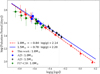 |
Fig. 2 Log-log plot of the pulsation period [days] versus the surface gravity, g [cgs], which follows a linear law whose parameters were computed with a non-linear least-squares method, given in Eqs. (1) and (2). |
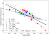 |
Fig. 3 Log-log plot of the pulsation period [days] versus the effective temperature, Teff [K], which is in agreement with photosphere dynamics. We notice two groups of data (above and below the black curve) that are not linked to mass. The linear relation is given in Eq. (3). |
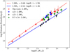 |
Fig. 4 Log-log of the pulsation period [days] versus the stellar radius R★[R⊙], which is in agreement with photosphere dynamics. The linear laws’ expressions are given in Eqs. (4) and (5). |
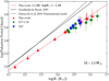 |
Fig. 5 Case of the 1.0 M⊙ simulations: Log-log of the pulsation period [days] versus the stellar radius, R★[R⊙]. We compare the analytical law established here (dashed red curve) with the law from Vassiliadis & Wood (1993) (black curve) and with the fundamental mode from Trabucchi et al. (2019) (dashed black curve). Overall, we found similar trends, only separated by an offset. The pulsation periods of the simulations are shorter than expected. |
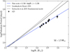 |
Fig. 6 Case of the 1.5 M⊙ simulations: same as in Fig. 5. In this case, the mass appears in the equations from Trabucchi et al. (2019) as its logarithm does not equal zero anymore. |
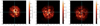 |
Fig. 7 Temporal evolution of an AGB simulation. The intensity maps are in erg · s−1 · Å−1. The star indicates the position of the photocentre at the given time for the simulation st28gm05n028. The dashed lines intersect at the geometric centre of the image. |
2.3 Photocentre variability of the RHD simulations in the Gaia G band
For each intensity map computed (for example, Fig. 7), we calculated the position of the photocentre as the intensity-weighted mean of the x-y positions of all emitting points tiling the visible stellar surface according to
 (6)
(6)
 (7)
(7)
where I(i, j) is the emerging intensity for the grid point (i, j) with co-ordinates x(i, j), y(i, j) and N the number of points in each co-ordinate of the simulated box.
Large-scale convective cells drag hot plasma from the core towards the surface, where it cools down and sinks (Freytag et al. 2017). Coupled with pulsations, this causes optical depth and brightness temporal and spatial variability, moving the photocen-tre position (Chiavassa et al. 2011, 2018). Thus, in the presence of brightness asymmetries, the photocentre will not coincide with the barycentre of the star. Figure 7 displays the time variability of the photocentre position (blue star) for three snapshots of the simulation st28gm05n028. The dashed lines intersect at the geometric centre of the image.
We computed the time-averaged photocentre position, 〈Px〉 and 〈Py〉, for each Cartesian co-ordinate in astronomical units, [AU], the time-averaged radial photocentre position, 〈P〉 as 〈P〉 = (〈Px〉2 + 〈Py〉2)1/2, and its standard deviation, σP, in AU and as a percentage of the corresponding stellar radius, R★ [% of R★] (see Table A.1).
Figure 8 displays the photocentre displacement over the total duration for the simulation st28gm05n028, with the average position as the red dot and σP as the red circle radius (see additional simulations in Figs. B1–B21, available on Zenodo2).
We also computed the histogram of the radial position of the photocentre for every snapshot available of every simulation (Fig. 9). The radial position is defined as  in % of R★. We notice that the photocentre is mainly situated between 0.05 and 0.15 of the stellar radius.
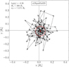 |
Fig. 8 Temporal evolution of the photocentre displacement for an AGB simulation, here st28gm05n028, same as in Fig. 7. The dashed lines intersect at the geometric centre of the image. The red dot indicates the average position of the photocentre and the red circle its standard deviation. |
2.4 Correlation between the photocentre displacement and the stellar parameters
After the correlations between Ppuls and the stellar parameters (log(g), Teff and R★), we studied correlations between Ppuls and the photocentre displacement, σP, displayed in Fig. 10. The pulsation period increases when the surface gravity decreases (Fig. 2); in other words, when the stellar radius increases. The photocentre gets displaced across larger distances (Chiavassa et al. 2018). We notice a correlation for each sub-group that we approximated with a power law, whose parameters were determined with a non-linear least-squares method (see Eqs. (8) and (9)):
 (8)
(8)
 (9)
(9)
The resulting reduced  are
are  and
and  . As before, we note a stark difference because there are fewer 1.5 M⊙ simulations and they are less scattered.
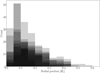 |
Fig. 9 Histograms of the radial positions of the photocentre for all the intensity maps we computed and used in this work. The darker the shadow, the more often the photocentre is situated in the associated bin. Overall, we notice the photocentre is situated between 5 and 15% of the stellar radius. |
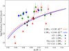 |
Fig. 10 Pulsation period in logarithmic scale versus the photocentre displacement for the 31 models. We group the models whether their mass is equal to 1.0 M⊙ or 1.5 M⊙. We approximate our data by a power law, one for each group (see Eqs. (8) and (9)). |
3 Comparison with observations from the Gaia mission
From the RHD simulations, we found analytical laws between the pulsation period and stellar parameters and between the pulsation period and the photocentre displacement, which were used to estimate the uncertainties of the results. We used these laws with the parallax uncertainty, σϖ, measured by Gaia to derive the stellar parameters of observed stars.
3.1 Selection of the sample
To compare the analytical laws with observational data, the parameters of the observed stars need to match the parameters of the simulations. Uttenthaler et al. (2019) investigated the interplay between mass-loss and third dredge-up (3DUP) of a sample of variable stars in the solar neighbourhood, which we further constrained to select suitable stars for our analysis by following these conditions: (i) Mira stars with an assumed solar metallicity, (ii) a luminosity, L★, lower than 10000 L⊙, and  being the uncertainty on the luminosity, and (iii) the GDR3 parallax uncertainty, σϖ, lower than 0.14 mas. We also selected stars whose (iv) renormalised unit weight error (RUWE) is lower than 1.4 (Andriantsaralaza et al. 2022). This operation resulted in a sample of 53 Mira stars (Table A.2).
The pulsation periods were taken mainly from Templeton et al. (2005) where available, or were also collected from VizieR. Preference was given to sources with available light curves that allowed for a critical evaluation of the period, such as the All Sky Automated Survey (Pojmanski 1998). Since some Miras have pulsation periods that change significantly in time (Wood & Zarro 1981; Templeton et al. 2005), we also analysed visual photometry from the AAVSO3 database and determined present-day periods with the program Period044 (Lenz & Breger 2005). The analysis of Merchan-Benitez et al. (2023) provided a period variability of the order of 2.4% of the respective pulsation period for Miras in the solar neighbourhood.
The luminosities were determined from a numerical integration under the photometric spectral energy distribution between the B-band at the short end and the IRAS 60 µm band or, if available, the Akari 90 µm band. A linear extrapolation to λ = 0 and ν = 0 was taken into account. The photometry was corrected for interstellar extinction using the map of Gontcharov (2017). We adopted the GEDR3 parallaxes and applied the average zero-point offset of quasars found by Lindegren et al. (2021): −21 mas. Two main sources of uncertainty on the luminosity are the parallax uncertainty and the intrinsic variability of the stars. The uncertainty on interstellar extinction and on the parallax zero-point were neglected.
The RUWE5 is expected to be around 1 0 for sources where the single-star model provides a good fit to the astrometric observations. Following Andriantsaralaza et al. (2022), we rejected stars whose RUWE is above 1 4 as their astrometric solution is expected to be poorly reliable and may indicate unresolved binaries.
Figure 11 displays the location of stars in a pulsation period-luminosity diagram with the colour scale indicating the number of good along-scan observations – that is, astromet-ric_n_good_obs_al data from GDR3 (top panel) – or indicating the RUWE (bottom panel). We investigated whether the number of times a star is observed, Nobs, or the number of observed periods, Nper, is correlated with RUWE. We do not see improvements of the astrometric solution when more observations are used to compute it.
Information about the third dredge-up activity of the stars is available from spectroscopic observations of the absorption lines of technetium (Tc, see Uttenthaler et al. 2019). Tc-rich stars have undergone a third dredge-up event and are thus more evolved and/or more massive than Tc-poor stars. Also, since 12C is dredged up along with Tc, the C/O ratio could be somewhat enhanced in the Tc-rich compared to the Tc-poor stars. However, as our subsequent analysis showed, we do not find significant differences between Tc-poor and Tc-rich stars with respect to their astrometric characteristics; hence, this does not impact our results.
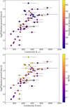 |
Fig. 11 Pulsation period in logarithmic scale [days] of the sample versus their luminosity, [L⊙]. Top panel: number of observations in colour scale. Bottom panel: RUWE in colour scale. |
3.2 Origins of the parallax uncertainty
The uncertainty in Gaia parallax measurements has multiple origins: (i) instrumental (Lindegren et al. 2021), (ii) distance (Lindegren et al. 2021), and (iii) convection-related (Chiavassa et al. 2011, 2018, 2022). This makes the error budget difficult to estimate. In particular, only with time-dependent parallaxes with Gaia Data Release 4 will the convection-related part be definitively characterised (Chiavassa et al. 2019). Concerning the distance and instrumental parts, Lindegren et al. (2021) investigated the bias of the parallax versus magnitude, colour, and position and developed an analytic method to correct the parallax of these biases. For comparison, the parallax and the corrected parallax are displayed in Table A.2, columns 8 and 9, respectively. In this work, we assume that convective-related variability is the main contributor to the parallax uncertainty budget, which is already hinted at in observations; thus, σP is equivalent to σϖ.
Indeed, optical interferometric observations of an AGB star showed the presence of large convective cells that affected the photocentre position. It has been shown for the same star that the convection-related variability accounts for a substantial part of the Gaia Data Release 2 parallax error (see in particular Fig. 2, Chiavassa et al. 2020).
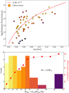 |
Fig. 12 Comparison of the pulsation period of the sample between observations and estimations from the simulations where M★ = 1. 0 M⊙. Top panel: pulsation period, Pobs, in logarithmic scale versus the parallax uncertainty of the observed sample, the dashed red curve being the Eq. (8) inferred from the analysis of the 1.0 M⊙ simulations. The colours represent the relative difference between the pulsation period calculated from Eq. (8) and the observations. Bottom panel: histogram of these relative differences. The red line accounts for the cumulative number of stars in the respective and preceding bins (see right-hand Y-axis). The limits of the last bin are 60 and 73%, with only one star above 70%. |
3.3 Retrieval of the surface gravity based on the analytical laws
In Section 2.4, we established an analytical law, Eq. (8), between σP and Ppuls with the 1.0 M⊙ simulations. We used it to calculate the pulsation period, P1.0, of the stars from observed σϖ. We defined ∆P1.0, the relative difference between the observed pulsation period, Pobs, and our results as  . This intermediate step gives an estimation of the error when computing the pulsation period and comparing it with observations. This error can then be used as a guideline to estimate the uncertainties of the final results; in other words, of the effective temperature, the surface gravity, and the radius of the stars in our sample.
The top panel of Figure 12 displays Pobs versus σϖ as dots and P1.0 versus σϖ as the dashed red curve. The bottom panel displays the histogram of the relative difference, ∆P1.0, and the cumulative percentage of the observed sample. The same colour scale is used in both panels: for example, light yellow represents a relative difference between P1.0 and Pobs of less than 5%, while purple represents a relative difference greater than 60% (column 3 in Table A.3).
∆P1.0 ranges from 0.4 to 72%, with a median of 16% (i.e. from 1 to 68 days’ difference). For 85% of the sample stars, ∆P1.0 is ≤30%, and for 57%, it is ≤20%, suggesting we statistically have a good agreement between our model results and the observations.
We then combined Eqs. (8) and (1) to derive the surface gravity (log(g1.0)) directly from σϖ (column 6 in Table A.3). The top left panel of Figure 13 displays log(Pobs) versus log(g1.0) and Eq. (1) as the dashed red curve. We notice that the calculated log(g1.0) values follow the same trend as log(g) from the simulations and are the most accurate when closest to the line.
We performed the same analysis with the analytical laws from the 1.5 M⊙ simulations. The top panel of Figure 14 displays the calculated P1.5 versus σϖ and the bottom panel displays a histogram of the relative difference between P1.5 and Pobs defined as ∆P1.5 (column 5 in Table A.3). The same colour code is used in both panels. We combined Eqs. (9) and (2) to compute log(g1.5). Fig. 13 displays log(Pobs) from the simulations versus log(g1.5).
For the 1.5 M⊙ simulations, ∆P1.5 ranges from 0.6 to 62%, with a median of 16% (i.e. from 1 to 76 days’ difference). For 81% of the sample stars, ∆P1.5 is ≤30%, and for 70%, it is ≤ 20%.
Qualitatively, we observe two different analytical laws depending on the mass of the models used to infer the laws. However, a larger grid of simulations, covering the mass range of AGB stars, would help to confirm this trend, tailor the analytical laws to specific stars, and predict more precise stellar parameters.
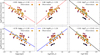 |
Fig. 13 Pulsation period from the observations versus stellar parameter values obtained from the simulations. Top row: pulsation period versus log(g) (left column), log(R★) (central column), log(Teff) (right column), each computed thanks to the analytical laws derived from the 1.0 M⊙ simulations. Bottom row: same as in the top row for the 1.5 M⊙ simulations. The equation of each law is given in the legend and is reported in Fig. 15. The colour scale used is the same as in Figs. 12 and 14. |
3.4 Retrieval of the other stellar parameters
We repeated the same procedure to retrieve the stellar radius, R1.0, and the effective temperature, T1.0 (columns 8 and 10 in Table A.3). Combining Eqs. (8) and (4), we computed the radius, R1.0. The top central panel of Figure 13 displays log(Pobs) versus log(R1.0). Combining the Eqs. (8) and (3), we computed the effective temperature, T1.0 (Fig. 13, top right panel). As in Section 3.3 for log(g1.0), the calculated log(R1.0) follow the Eq. (4) derived from the simulations, and log(R1.0) follow Eq. (3).
We repeated the same procedure for the 1.5 M⊙ simulations to retrieve R1.5 and T1.5 (columns 9 and 11 in Table A.1). The results are displayed in the bottom central and right panels of Fig. 13.
For comparison, R Peg has been observed with the interferometric instrument GRAVITY/VLTI in 2017, which provided a direct estimation of its radius:  (Wittkowski et al. 2018). From our study,
  and
and  , which is in good agreement with the results of Wittkowski et al. (2018). With future interferometric observations, we shall be able to further validate our results.
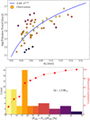 |
Fig. 14 Comparison of the pulsation period of the sample between observations and estimations from the simulations where M★ = 1.5 M⊙. Top panel: pulsation period, Pobs, in logarithmic scale versus the parallax uncertainty of the observed sample, the blue curve being the Eq. (9) inferred from the analysis of the 1.5 M⊙ simulations. The colours represent the relative difference between the pulsation period calculated from Eq. (9) and with the observations. Bottom panel: histogram of these relative differences. The red line accounts for the cumulative number of stars in the respective and preceding bins (see right-hand Y-axis). |
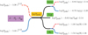 |
Fig. 15 Summary of the analytical laws we established. The dashed red lines correspond to the analysis when using only the 1.0 M⊙ simulations, the blue lines the analysis when using only the 1.5 M⊙ simulations. For the correlation between the pulsation period and the effective temperature, all available simulations were used. In the left part, we have the laws between the photocentre displacement and the pulsation period from the simulations. We assume that the parallax uncertainty, σϖ, is equivalent to σP as σP is the main contributor of the σϖ budget. In the right part, we have the laws between the pulsation period and the stellar parameters (log(g), Teff, R★). Combining these laws provides the parameters of the Mira stars based on the parallax uncertainty. The relative difference between the calculated and the observational pulsation periods can be used to estimate the uncertainties of the stellar parameters. |
4 Summary and conclusions
We computed intensity maps in the Gaia band from the snapshots of 31 RHD simulations of AGB stars computed with CO5BOLD. The standard deviation of the photocentre displacement, σP, due to the presence of large convective cells on the surface, ranges from about 4% to 13% of its corresponding stellar radius, which is coherent with previous studies and is non-negligible in photometric data analysis. It becomes the main contributor to the Gaia parallax uncertainty σϖ budget. The dynamics and winds of the AGB stars also affect the determination of stellar parameters and amplify their uncertainties. It becomes worth exploring the correlations between all these aspects to eventually retrieve such parameters from the parallax uncertainty.
We provided correlations between the photocentre displacement and the pulsation period as well as between the pulsation period and stellar parameters: the effective surface gravity, log(g), the effective temperature, Teff, and the radius, R★. We separated the simulations into two sub-groups based on whether their mass is equal to 1.0 or 1.5 M⊙. Indeed, the laws we provided, and the final results, are sensitive to the mass. A grid of simulations covering a larger range of masses, with a meaningful number of simulations for each, would help confirm this observation and establish laws that are suitable for varied stars. This will be done in the future.
We then applied these laws to a sample of 53 Mira stars matching the simulations’ parameters. We first compared the pulsation period with the literature: we obtained a relative error of less than 30% for 85% of the stars in the sample for the first case and 81% for the second, which indicates reasonable results from a statistical point of view. This error can then be used as a guideline to estimate the uncertainties of the final results. We then computed log(g), Teff and R★ by combining the analytical laws (Table A.3).
While mass loss from red giant branch stars should be mainly independent of metallicity, it has been suggested that this is less true for AGB stars (McDonald & Zijlstra 2015). Photocen-tre displacement and stellar parameters may be dependent on metallicity and this question needs to be further studied.
We argue that the method used for Mira stars presented in this article, based on RHD simulations, can be generalised to any AGB stars whose luminosity is in the 2000–10 000 L⊙ range and that have a Gaia parallax uncertainty below 0.14 mas. Figure 15 sums up the analytical laws found in this work that can be used to calculate the stellar parameters.
Overall, we have demonstrated the feasibility of retrieving stellar parameters for AGB stars using their uncertainty on the parallax, thanks to the employment of state-of-the-art 3D RHD simulations of stellar convection. The future Gaia Data Release 4 will provide time-dependent parallax measurements, allowing one to quantitatively determine the photocentre-related impact on the parallax error budget and to directly compare the convection cycle, refining our understanding of AGB dynamics.
Data availability
Appendix B is available at https://zenodo.org/records/12802110
Acknowledgements
This work is funded by the French National Research Agency (ANR) project PEPPER (ANR-20-CE31-0002). BF acknowledges funding from the European Research Council (ERC) under the European Union’s Horizon 2020 research and innovation programme Grant agreement No. 883867, project EXWINGS. The computations were enabled by resources provided by the Swedish National Infrastructure for Computing (SNIC). This work was granted access to the HPC resources of Observatoire de la Côte d’Azur - Mésocentre SIGAMM.
Appendix A Tables
RHD simulation parameters.
Parameters of the sample Miras.
Stellar parameters of the Miras inferred from the simulations.
Appendix C M dwarfs versus AGB stars parallax uncertainty
Our key assumption is that the parallax uncertainty budget in the Mira sample is dominated by the photocentre shift due to the huge AGB convection cells. To test this assumption, one would need a comparison sample of stars with similar properties such as apparent G magnitude, distance, GBP – GRP colour, etc., but ideally without surface brightness inhomogeneities. M-type dwarfs could be useful for a comparison because they have similar GBP – GRP colour as our Miras. Therefore, we searched the SIMBAD database for M5 dwarfs with G < 15 mag, which yielded a sample of 240 objects. The list was cross-matched with the Gaia DR3 catalogue. Obvious misidentifications between SIMBAD and Gaia with G > 15 were culled from the list. A Hertzsprung-Russell diagram based on MG vs. GBP – GRP revealed that the sample still contained several misclassified M-type giant stars. Removing them retained a sample of 99 dwarf stars that have comparable GBP – GRP colour to the Miras sample. However, as M dwarfs are intrinsically much fainter than Miras, the dwarf stars are much closer to the sun than the Miras: their distances vary between ~ 7 and 160 pc, whereas our Mira sample stars are located between 300 and over 5000 pc from the sun. Furthermore, we noticed that a significant fraction of the dwarfs have surprisingly large parallax uncertainties. These could be related to strong magnetic fields on the surfaces of these dwarfs that are the cause of bright flares or large, dark spots, creating surface brightness variations similar to those expected in the AGB stars. A detailed investigations into the reasons for their large parallax uncertainties is beyond the scope of this paper. We therefore decided to not do the comparison with the M dwarfs.
Luckily, the contaminant, misclassified (normal) M giants in the Simbad search appear to be a much better comparison sample. They have overlap with the Mira stars in G magnitude and are at fairly similar distances, between ~ 260 and 1700 pc. The only drawbacks are that the normal M giants are somewhat bluer in GBP – GRP colour than the Miras, and we found only ten suitable M giants in our limited search. Fig. C1 illustrates the location of the M giants together with the Mira sample and the M dwarfs in an HR diagram.
Importantly, we note that the parallax uncertainties of the M giants are all smaller than those of the Miras. This is shown in Fig. C2, where the logarithmic value of the parallax uncertainty is plotted as a function of the logarithm of the distance (here simply taken as the inverse of the parallax). On average, the M giants have parallax uncertainties that are smaller by a factor of 3.5 than those of the Miras. As the M giants are more compact than the Miras and have smaller pressure scale heights, it is plausible that the larger parallax uncertainties of the Miras indeed result from their surface convection cells. We therefore conclude that our key assumption is correct.
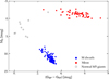 |
Fig. C1 Hertzsprung-Russell diagram: absolute G magnitude MG versus GBP – GRP colour from Gaia data. In red are the Mira stars of our sample, in blue the M5 dwarfs, and in white the misclassified (normal) M giants. |
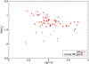 |
Fig. C2 Log-log of the parallax uncertainty, σϖ, versus the distance, simply taken as the inverse of the parallax, ϖ. We see that the M giants parallax uncertainties are smaller than those of the Miras by a factor of ~ 3.5. |
References
- Ahmad, A., Freytag, B., & Höfner, S. 2023, A&A, 669, A49 [NASA ADS] [CrossRef] [EDP Sciences] [Google Scholar]
- Andriantsaralaza, M., Ramstedt, S., Vlemmings, W. H. T., & De Beck, E. 2022, A&A, 667, A74 [NASA ADS] [CrossRef] [EDP Sciences] [Google Scholar]
- Asplund, M., Grevesse, N., Sauval, A. J., & Scott, P. 2009, ARA&A, 47, 481 [NASA ADS] [CrossRef] [Google Scholar]
- Chen, D.-C., Xie, J.-W., Zhou, J.-L., et al. 2021, ApJ, 909, 115 [NASA ADS] [CrossRef] [Google Scholar]
- Chiavassa, A., Plez, B., Josselin, E., & Freytag, B. 2009, A&A, 506, 1351 [NASA ADS] [CrossRef] [EDP Sciences] [Google Scholar]
- Chiavassa, A., Pasquato, E., Jorissen, A., et al. 2011, A&A, 528, A120 [NASA ADS] [CrossRef] [EDP Sciences] [Google Scholar]
- Chiavassa, A., Freytag, B., & Schultheis, M. 2018, A&A, 617, L1 [NASA ADS] [CrossRef] [EDP Sciences] [Google Scholar]
- Chiavassa, A., Freytag, B., & Schultheis, M. 2019, Proceedings of the Annual meeting of the French Society of Astronomy and Astrophysics [Google Scholar]
- Chiavassa, A., Kravchenko, K., Millour, F., et al. 2020, A&A, 640, A23 [NASA ADS] [CrossRef] [EDP Sciences] [Google Scholar]
- Chiavassa, A., Kudritzki, R., Davies, B., Freytag, B., & de Mink, S. E. 2022, A&A, 661, L1 [NASA ADS] [CrossRef] [EDP Sciences] [Google Scholar]
- De Beck, E., Decin, L., de Koter, A., et al. 2010, A&A, 523, A18 [NASA ADS] [CrossRef] [EDP Sciences] [Google Scholar]
- Decin, L. 2021, ARA&A, 59, 337 [NASA ADS] [CrossRef] [Google Scholar]
- Freytag, B. 2013, Mem. Soc. Astron. Ital. Suppl., 24, 26 [Google Scholar]
- Freytag, B. 2017, Mem. Soc. Astron. Ital., 88, 12 [Google Scholar]
- Freytag, B., & Höfner, S. 2023, A&A, 669, A155 [NASA ADS] [CrossRef] [EDP Sciences] [Google Scholar]
- Freytag, B., Holweger, H., Steffen, M., & Ludwig, H. G. 1997, Proceedings of the ESO Workshop, 316 [Google Scholar]
- Freytag, B., Steffen, M., Ludwig, H. G., et al. 2012, J. Comput. Phys., 231, 919 [Google Scholar]
- Freytag, B., Liljegren, S., & Höfner, S. 2017, A&A, 600, A137 [NASA ADS] [CrossRef] [EDP Sciences] [Google Scholar]
- Gaia Collaboration (Prusti, T., et al.) 2016, A&A, 595, A1 [NASA ADS] [CrossRef] [EDP Sciences] [Google Scholar]
- Gaia Collaboration (Vallenari, A., et al.) 2023, A&A, 674, A1 [NASA ADS] [CrossRef] [EDP Sciences] [Google Scholar]
- Gontcharov, G. A. 2017, Astron. Lett., 43, 472 [NASA ADS] [CrossRef] [Google Scholar]
- Gustafsson, B., Edvardsson, B., Eriksson, K., et al. 2008, A&A, 486, 951 [NASA ADS] [CrossRef] [EDP Sciences] [Google Scholar]
- Höfner, S., & Olofsson, H. 2018, A&A Rev., 26, 1 [CrossRef] [Google Scholar]
- Lenz, P., & Breger, M. 2005, Commun. Asteroseismol., 146, 53 [Google Scholar]
- Lindegren, L., Bastian, U., Biermann, M., et al. 2021, A&A, 649, A4 [EDP Sciences] [Google Scholar]
- McDonald, I., & Zijlstra, A. A. 2015, MNRAS, 448, 502 [Google Scholar]
- Merchan-Benitez, P., Uttenthaler, S., & Jurado-Vargas, M. 2023, A&A, 672, A165 [NASA ADS] [CrossRef] [EDP Sciences] [Google Scholar]
- Pojmanski, G. 1998, Acta Astron., 48, 35 [Google Scholar]
- Templeton, M. R., Mattei, J. A., & Willson, L. A. 2005, AJ, 130, 776 [NASA ADS] [CrossRef] [Google Scholar]
- Trabucchi, M., Wood, P. R., Montalbán, J., et al. 2019, MNRAS, 482, 929 [Google Scholar]
- Uttenthaler, S., McDonald, I., Bernhard, K., Cristallo, S., & Gobrecht, D. 2019, A&A, 622, A120 [NASA ADS] [CrossRef] [EDP Sciences] [Google Scholar]
- Vassiliadis, E., & Wood, P. R. 1993, ApJ, 413, 641 [Google Scholar]
- Wittkowski, M., Rau, G., Chiavassa, A., et al. 2018, A&A, 613, L7 [NASA ADS] [CrossRef] [EDP Sciences] [Google Scholar]
- Wood, P. R., & Zarro, D. M. 1981, ApJ, 247, 247 [NASA ADS] [CrossRef] [Google Scholar]
GDR3 website: https://www.cosmos.esa.int/web/gaia/data-release-3
https://gea.esac.esa.int/archive/documentation/GDR2/, Part V, Chapter 14.1.2
All Tables
All Figures
|
Fig. 1 Log-log plot of the surface gravity [cgs] versus the pressure scale height [cm]. As the effective temperature is near constant among all our models, we expect a linear relation. |
| In the text | |
|
Fig. 2 Log-log plot of the pulsation period [days] versus the surface gravity, g [cgs], which follows a linear law whose parameters were computed with a non-linear least-squares method, given in Eqs. (1) and (2). |
| In the text | |
|
Fig. 3 Log-log plot of the pulsation period [days] versus the effective temperature, Teff [K], which is in agreement with photosphere dynamics. We notice two groups of data (above and below the black curve) that are not linked to mass. The linear relation is given in Eq. (3). |
| In the text | |
|
Fig. 4 Log-log of the pulsation period [days] versus the stellar radius R★[R⊙], which is in agreement with photosphere dynamics. The linear laws’ expressions are given in Eqs. (4) and (5). |
| In the text | |
|
Fig. 5 Case of the 1.0 M⊙ simulations: Log-log of the pulsation period [days] versus the stellar radius, R★[R⊙]. We compare the analytical law established here (dashed red curve) with the law from Vassiliadis & Wood (1993) (black curve) and with the fundamental mode from Trabucchi et al. (2019) (dashed black curve). Overall, we found similar trends, only separated by an offset. The pulsation periods of the simulations are shorter than expected. |
| In the text | |
|
Fig. 6 Case of the 1.5 M⊙ simulations: same as in Fig. 5. In this case, the mass appears in the equations from Trabucchi et al. (2019) as its logarithm does not equal zero anymore. |
| In the text | |
|
Fig. 7 Temporal evolution of an AGB simulation. The intensity maps are in erg · s−1 · Å−1. The star indicates the position of the photocentre at the given time for the simulation st28gm05n028. The dashed lines intersect at the geometric centre of the image. |
| In the text | |
|
Fig. 8 Temporal evolution of the photocentre displacement for an AGB simulation, here st28gm05n028, same as in Fig. 7. The dashed lines intersect at the geometric centre of the image. The red dot indicates the average position of the photocentre and the red circle its standard deviation. |
| In the text | |
|
Fig. 9 Histograms of the radial positions of the photocentre for all the intensity maps we computed and used in this work. The darker the shadow, the more often the photocentre is situated in the associated bin. Overall, we notice the photocentre is situated between 5 and 15% of the stellar radius. |
| In the text | |
|
Fig. 10 Pulsation period in logarithmic scale versus the photocentre displacement for the 31 models. We group the models whether their mass is equal to 1.0 M⊙ or 1.5 M⊙. We approximate our data by a power law, one for each group (see Eqs. (8) and (9)). |
| In the text | |
|
Fig. 11 Pulsation period in logarithmic scale [days] of the sample versus their luminosity, [L⊙]. Top panel: number of observations in colour scale. Bottom panel: RUWE in colour scale. |
| In the text | |
|
Fig. 12 Comparison of the pulsation period of the sample between observations and estimations from the simulations where M★ = 1. 0 M⊙. Top panel: pulsation period, Pobs, in logarithmic scale versus the parallax uncertainty of the observed sample, the dashed red curve being the Eq. (8) inferred from the analysis of the 1.0 M⊙ simulations. The colours represent the relative difference between the pulsation period calculated from Eq. (8) and the observations. Bottom panel: histogram of these relative differences. The red line accounts for the cumulative number of stars in the respective and preceding bins (see right-hand Y-axis). The limits of the last bin are 60 and 73%, with only one star above 70%. |
| In the text | |
|
Fig. 13 Pulsation period from the observations versus stellar parameter values obtained from the simulations. Top row: pulsation period versus log(g) (left column), log(R★) (central column), log(Teff) (right column), each computed thanks to the analytical laws derived from the 1.0 M⊙ simulations. Bottom row: same as in the top row for the 1.5 M⊙ simulations. The equation of each law is given in the legend and is reported in Fig. 15. The colour scale used is the same as in Figs. 12 and 14. |
| In the text | |
|
Fig. 14 Comparison of the pulsation period of the sample between observations and estimations from the simulations where M★ = 1.5 M⊙. Top panel: pulsation period, Pobs, in logarithmic scale versus the parallax uncertainty of the observed sample, the blue curve being the Eq. (9) inferred from the analysis of the 1.5 M⊙ simulations. The colours represent the relative difference between the pulsation period calculated from Eq. (9) and with the observations. Bottom panel: histogram of these relative differences. The red line accounts for the cumulative number of stars in the respective and preceding bins (see right-hand Y-axis). |
| In the text | |
|
Fig. 15 Summary of the analytical laws we established. The dashed red lines correspond to the analysis when using only the 1.0 M⊙ simulations, the blue lines the analysis when using only the 1.5 M⊙ simulations. For the correlation between the pulsation period and the effective temperature, all available simulations were used. In the left part, we have the laws between the photocentre displacement and the pulsation period from the simulations. We assume that the parallax uncertainty, σϖ, is equivalent to σP as σP is the main contributor of the σϖ budget. In the right part, we have the laws between the pulsation period and the stellar parameters (log(g), Teff, R★). Combining these laws provides the parameters of the Mira stars based on the parallax uncertainty. The relative difference between the calculated and the observational pulsation periods can be used to estimate the uncertainties of the stellar parameters. |
| In the text | |
|
Fig. C1 Hertzsprung-Russell diagram: absolute G magnitude MG versus GBP – GRP colour from Gaia data. In red are the Mira stars of our sample, in blue the M5 dwarfs, and in white the misclassified (normal) M giants. |
| In the text | |
|
Fig. C2 Log-log of the parallax uncertainty, σϖ, versus the distance, simply taken as the inverse of the parallax, ϖ. We see that the M giants parallax uncertainties are smaller than those of the Miras by a factor of ~ 3.5. |
| In the text | |
Current usage metrics show cumulative count of Article Views (full-text article views including HTML views, PDF and ePub downloads, according to the available data) and Abstracts Views on Vision4Press platform.
Data correspond to usage on the plateform after 2015. The current usage metrics is available 48-96 hours after online publication and is updated daily on week days.
Initial download of the metrics may take a while.