| Issue |
A&A
Volume 617, September 2018
|
|
|---|---|---|
| Article Number | L1 | |
| Number of page(s) | 6 | |
| Section | Letters to the Editor | |
| DOI | https://doi.org/10.1051/0004-6361/201833844 | |
| Published online | 12 September 2018 | |
Letter to the Editor
Heading Gaia to measure atmospheric dynamics in AGB stars
1
Université Côte d’Azur, Observatoire de la Côte d’Azur, CNRS, Lagrange, CS 34229, Nice, France
e-mail: This email address is being protected from spambots. You need JavaScript enabled to view it.
2
Department of Physics and Astronomy at Uppsala University, Regementsvägen 1, Box 516, 75120 Uppsala, Sweden
Received:
13
July
2018
Accepted:
7
August
2018
Abstract
Context. Asymptotic giant branch (AGB) stars are characterised by complex stellar surface dynamics that affect the measurements and amplify the uncertainties on stellar parameters. The uncertainties in observed absolute magnitudes have been found to originate mainly from uncertainties in the parallaxes. The resulting motion of the stellar photocentre could have adverse effects on the parallax determination with Gaia.
Aims. We explore the impact of the convection-related surface structure in AGBs on the photocentric variability. We quantify these effects to characterise the observed parallax errors and estimate fundamental stellar parameters and dynamical properties.
Methods. We use three-dimensional (3D) radiative hydrodynamics simulations of convection with CO5BOLD and the post-processing radiative transfer code OPTIM3D to compute intensity maps in the Gaia G band [325–1030 nm]. From those maps, we calculate the intensity-weighted mean of all emitting points tiling the visible stellar surface (i.e. the photocentre) and evaluate its motion as a function of time. We extract the parallax error from Gaia data-release 2 (DR2) for a sample of semi-regular variables in the solar neighbourhood and compare it to the synthetic predictions of photocentre displacements.
Results. AGB stars show a complex surface morphology characterised by the presence of few large-scale long-lived convective cells accompanied by short-lived and small-scale structures. As a consequence, the position of the photocentre displays temporal excursions between 0.077 and 0.198 AU (≈5 to ≈11% of the corresponding stellar radius), depending on the simulation considered. We show that the convection-related variability accounts for a substantial part of the Gaia DR2 parallax error of our sample of semi-regular variables. Finally, we present evidence for a correlation between the mean photocentre displacement and the stellar fundamental parameters: surface gravity and pulsation. We suggest that parallax variations could be exploited quantitatively using appropriate radiation-hydrodynamics (RHD) simulations corresponding to the observed star.
Key words: stars: atmospheres / stars: AGB and post-AGB / astrometry / parallaxes / hydrodynamics
© ESO 2018
 Open Access article, published by EDP Sciences, under the terms of the Creative Commons Attribution License (http://creativecommons.org/licenses/by/4.0), which permits unrestricted use, distribution, and reproduction in any medium, provided the original work is properly cited.
1. Introduction
Low- to intermediate-mass stars evolve to red giant and asymptotic giant branch increasing the mass-loss during this evolution. They are characterised: (i) by large-amplitude variations in radius, brightness, and temperature of the star; and (ii) by a strong mass-loss rate driven by an interplay between pulsation, dust formation in the extended atmosphere, and radiation pressure on the dust (Höfner & Olofsson 2018). Their complex dynamics affect the measurements and amplify the uncertainties on stellar parameters.
Gaia (Gaia Collaboration 2016) is an astrometric, photometric, and spectroscopic space-borne mission. It performs a survey of a large part of the Milky Way. The second data release (Gaia DR2) in April 2018 (Gaia Collaboration 2018) brought high-precision astrometric parameters (i.e. positions, parallaxes, and proper motions) for over 1 billion sources brighter that G ≈ 20. Among all the objects that have been observed, the complicated atmospheric dynamics of asymptotic giant branch (AGB) stars affect the photocentric position and, in turn, their parallaxes (Chiavassa et al. 2011). The convection-related variability, in the context of Gaia astrometric measurements, can be considered as “noise” that must be quantified in order to better characterise any resulting error on the parallax determination. However, important information about stellar properties, such as the fundamental stellar parameters, may be hidden behind the Gaia measurement uncertainty.
RHD simulation parameters.
In this work we explore the effect of convection-related surface structures on the photocentre to estimate its impact on the Gaia astrometric measurements.
2. Methods
We used the radiation-hydrodynamics (RHD) simulations of AGB stars (Freytag et al. 2017) computed with CO5BOLD (Freytag et al. 2012) code. The code solves the coupled non-linear equations of compressible hydrodynamics and non-local radiative energy transfer in the presence of a fixed external spherically symmetric gravitational field in a three-dimensional (3D) cartesian grid. It is assumed that solar abundances are appropriate for M-type AGB stars. The basic stellar parameters of the RHD simulations are reported in Table 1. The configuration used is the “star-in-a-box”, where the evolution of the outer convective envelope and the inner atmosphere of AGB stars are taken into account in the calculation. In the simulations, convection, waves, and shocks all contribute to the dynamical pressure and, therefore, to an increase of the stellar radius and to a levitation of material into layers where dust can form. No dust is included in any of the current models. The regularity of the pulsations decreases with decreasing gravity as the relative size of convection cells increases. The pulsation period is extracted with a fit of the Gaussian distribution in the power spectra of the simulations. The period of the dominant mode increase with the radius of the simulation (Table 1 in Freytag et al. 2017).
We computed intensity maps based on snapshots from the RHD simulations integrating in the Gaia G photometric system (Evans et al. 2018). For this purpose, we employed the code OPTIM3D (Chiavassa et al. 2009), which takes into account the Doppler shifts caused by the convective motions. The radiative transfer is computed in detail using pre-tabulated extinction coefficients per unit mass, as for MARCS (Gustafsson et al. 2008) as a function of temperature, density, and wavelength for the solar composition (Asplund et al. 2009). Micro-turbulence broadening was switched off. The temperature and density distributions are optimised to cover the values encountered in the outer layers of the RHD simulations.
The surface of the deep convection zone has large and small convective cells. The visible fluffy stellar surface is made of shock waves that are produced in the interior and are shaped by the top of the convection zone as they travel outward (Freytag et al. 2017). In addition to this, on the top of the convection-related surface structures, other structures appear. They result from the opacity effect and dynamics at Rosseland optical depths smaller than 1 (i.e. further up in the atmosphere with respect to the continuum-forming region). At the wavelengths in Gaia G-band, TiO molecules produce strong absorption. Both of these effects affect the position of the photocentre and cause temporal fluctuations during the Gaia mission, as already pointed out for red supergiant stars in Chiavassa et al. (2011). In the Gaia G photometric system (Fig. 1), the situation is analogous with a few large convective cells with sizes of a third of the stellar radii (i.e. ≈0.6 AU) that evolve on a scale of several months to a few years, as well as a few short-lived (weeks to month) convective cells at smaller scales (≲10% of the stellar radius)
We calculated the position of the photocentre for each map (i.e. as a function of time) as the intensity-weighted mean of the x − y positions of all emitting points tiling the visible stellar surface according to (1)
(1)
 (2)
(2)
where I(i,j) is the emerging intensity for the grid point (i, j) with coordinates x(i, j), y(i, j) of the simulation, and N = 281 is the total number of grid points in the simulated box. In the presence of surface brightness asymmetries, the photocentre position will not coincide with the barycentre of the star and its position will change as the surface pattern changes with time. This is displayed in the photocentre excursion plots (Figs. A.1–A.5) for each simulation in the Appendix together with the time-averaged photocentre position (⟨P⟩) and its standard deviations (σP) in Table 1. The value of σP (the third column from the right in Table 1) is mostly fixed by the short time scales corresponding to the small atmospheric structures. However, the fact that ⟨Px⟩ and ⟨Py⟩ do not average to zero (last two columns of Table 1 and, e.g. Fig. A.6 in the Appendix), means that the photocentre tends not to be centred most of the time on the nominal centre of the star, because of the presence of a large convective cell.
Depending on the simulation, σP varies between 0.077 and 0.198 AU (≈5 to ≈11% of the corresponding stellar radius). This measure of the mean photocentre noise induced by the stellar dynamics in the simulations is compared in the following section to Gaia measurement uncertainty to extract information on stellar parameters from the astrometric measurements. It should be noted that the main information that is used to determine the astrometric characteristics of every star will be the along-scan measurement of Gaia. Chiavassa et al. (2011) showed that the projection of the star position along the scanning direction of the satellite with respect to a known reference point discloses similar, though slightly increased, values of σP. At the current state of the DR2, it is not possible to perform this on the data and we assumed the conservative value of σP directly extracted from the RHD simulations for the following comparisons.
 |
Fig. 1. Example of the squared root intensity maps (the range is |
![Mathematical equation: $ \sqrt {[0. - 3000.]} $](/articles/aa/full_html/2018/09/aa33844-18/aa33844-18-eq1.gif)
3. Observations
Evolved late-type stars show convection-related variability that may be considered, in the context of Gaia astrometric measurement, as “noise”. Chiavassa et al. (2011) demonstrated that RHD simulations can account for a substantial part of the supplementary “cosmic noise” that affects Hipparcos measurements for some prototypical red supergiant stars. As a consequence, the convection-related noise has to be quantified in order to better characterise any resulting error on the parallax.
We extracted the parallax error (σϖ) from Gaia DR2 for a sample of semiregular variables (SRV) from Tabur et al. (2009), Glass & van Leeuwen (2007), and Jura et al. (1993) that match the theoretical luminosities of RHD simulations (Table 1). Moreover, we only considered stars with 4000 < L⊙< 8000 in order to compare with our simulations. It has to be noted that σϖ may still vary in the following data releases because: (i) the mean number of measurements for each source amounts to 26 (Mowlavi et al. 2018) and this number will be 70–80 in total at the end of the nominal mission; (ii) and new solutions may be applied to adjust the imperfect chromaticity correction (Arenou et al. 2018). We cross-identified our sample stars with the Gaia DR2 as well as with the distance catalogue of Bailer-Jones et al. (2018) that uses a weak distance prior, varying as a function of Galactic longitude and latitude, to derive distances for the Gaia DR21. The apparent K-band magnitudes were transformed to absolute K magnitudes using the Gaia distances of Bailer-Jones et al. (2018) and neglecting the interstellar absorption which should be very small in the local neighbourhood. The absolute K magnitudes were converted to bolometric magnitudes using the bolometric correction formula of Kerschbaum et al. (2010). The typical uncertainties in the bolometric correction (BCK) are of the order of ±0.1 mag. Finally, the bolometric magnitudes were converted to luminosities assuming a solar Mbol⊙ = 4.7 (Torres 2010). The error bars on luminosities were calculated using the upper and lower distance limits provided by Bailer-Jones et al. (2018) for each of our sources together with the error of ±0.1mag for BCK. We do not correct for the variation of the K-band light curve as only amplitudes in the visual are available and the K-band amplitude of AGB stars is in general much smaller than in the visual.
4. Comparison and predictions
AGB stars are characterised by complex stellar surface dynamics that affect the measurements and the determined stellar parameters. The uncertainties in observed absolute magnitudes have been shown to originate mainly from uncertainties in the parallaxes. In this section we investigate if the parallax errors of our SRV sample can be explained by the resulting motion of the stellar photocentre seen in the RHD simulations.
Figure 2 (left panel) displays the parallax errors against the luminosity and compares these results to the standard deviations of the photocentre displacement in the simulations. The latter show good agreement with the observations. There are two luminosity families in the 3D simulations. In general the more luminous models are larger, that is, they have lower surface gravity, which causes larger convection cells and a more “fluffy” atmosphere (Freytag et al. 2017). As a consequence, for the simulation with higher luminosity (≈7000 L⊙), the parallax error ratio, defined as ⟨σϖ⟩/σP (where ⟨σϖ⟩ is the average error for the stars with luminosity close enough to the corresponding simulation luminosity), is [0.75–0.98]. This attests that convection-related variability accounts for a substantial part of the parallax error in Gaia measurements. For lower luminosities (≈5000 L⊙), the ratio is [1.15–1.95], indicating that for those simulations the situation is less clear. However, the observed and simulated luminosities do not coincide exactly and the observed error bars are still very large. One limitation of the existing model grid is the restriction to 1 M⊙. In the future, there will be models with other masses available. For a better comparison, we need simulations and observations with known luminosities, masses, and radii; neither is trivial.
An important piece of information is indeed hidden in the Gaia measurement uncertainty: using the corresponding stellar parameters of the RHD simulations of Table 1, we plotted (Fig. 2) σP as a function of surface gravity (central panel) and pulsation (right panel). They display a correlation between the mean photocentre displacement and the stellar fundamental parameters. While effective temperature does not show particularly correlated points, simulations with lower surface gravity (i.e. more extended atmospheres) return larger excursions of the photocentre. This behaviour is explained by the correlation between the stellar atmospheric pressure scale height ( ) and the photocentre displacement (Freytag 2001; Ludwig 2006; Chiavassa et al. 2011).
One property of AGB stars that is well constrained by observations is the period–luminosity (P–L) relation. The uncertainties in the determination of this relation are mainly based on the calculation of the distances and on the different P–L relations used. Figure 2 (right panel) reveals the correlation between the photocentre displacement and the logarithm of the pulsation: larger values of σP correspond to longer pulsation periods. Global shocks induced by large-amplitude, radial, and fundamental-mode pulsations have an impact on the detailed stellar structure of the stellar atmosphere, together with small-scale shocks. Both contribute to the levitation of material and the detected photocentre displacement (Freytag et al. 2017). This result is likely associated with the P–L relation found by Freytag et al. (2017), who showed that the RHD simulations reproduce the correct period for a given luminosity compared to the observations of Whitelock et al. (2009). Given the fact that σP explains Gaia measurement uncertainties on the parallaxes (left panel), we suggest that parallax variations from Gaia measurements could be exploited quantitatively using appropriate RHD simulations. However, the parameter space in our simulations is still limited (Table 1). In the future we aim to extend our RHD simulations’ parameters to lower and higher luminosities (i.e. shorter and longer periods) which will enable a more quantitative comparison with respect to the upcoming Gaia data releases.
 |
Fig. 2. Left panel: luminosity against the parallax error of the observations (σϖ, circle symbol in black) and the standard deviation of the photocentre displacement for the RHD simulations of Table 1 (σP, star symbol in red). Central panel: σP against the surface gravity for the RHD simulations. Right panel: σP against the logarithm of the period. |
5. Summary and conclusions
We used the snapshots from RHD simulations of AGB stars to compute intensity maps in the Gaia G photometric system. The visible fluffy stellar surface is made of shock waves that are produced in the interior and are shaped by the top of the convection zone as they travel outward. The surface is characterised by the presence of few large and long-lived convective cells accompanied by short-lived and small-scale structures. As a consequence, the position of the photocentre is affected by temporal fluctuations.
We calculated the standard deviation of the photocentre excursion for each simulation and found that σP varies between 0.077 and 0.198 AU (≈5 to ≈11% of the corresponding stellar radius) depending on the simulation. We compared the measurement of the mean photocentre noise induced by the stellar dynamics in the simulations (σP) to the measurement uncertainty on the parallax of a sample of AGB stars in the solar neighbourhood cross-matched with data from the Gaia DR2. We found good agreement with observations, suggesting that convection-related variability accounts for a substantial part of the parallax error. It should be noted that σϖ may still vary in the following data releases due to the increase of Gaia’s measurements in number and further corrections to the parallax solution.
Here we present evidence for a correlation between the mean photocentre displacement and the stellar fundamental parameters: surface gravity and pulsation. Concerning the latter, we showed that larger values of σP correspond to longer pulsation periods. This result, associated with the P–L relation found by Freytag et al. (2017), and the good agreement between simulations and observations (σP vs. σϖ), suggest that parallax variations from Gaia measurements could be exploited quantitatively using appropriate RHD simulations corresponding to the observed star.
We used the TAP service at http://gaia.ari.uni-heidelberg.de/tap.html
Acknowledgments
This work has made use of data from the European Space Agency (ESA) mission Gaia (https://www.cosmos.esa.int/gaia), processed by the Gaia Data Processing and Analysis Consortium (DPAC, https://www.cosmos.esa.int/web/). Funding for the DPAC has been provided by national institutions, in particular the institutions participating in the Gaia Multilateral Agreement. AC et MS thank Patrick de Laverny for the enlightening discussions. The authors thank the referee for the helpful comments during the refereeing process.
References
- Arenou, F., Luri, X., Babusiaux, C., et al. 2018, A&A, 616, A17 [Google Scholar]
- Asplund, M., Grevesse, N., Sauval, A. J., & Scott, P. 2009, ARA&A, 47, 481 [NASA ADS] [CrossRef] [Google Scholar]
- Bailer-Jones, C. A. L., Rybizki, J., Fouesneau, M., Mantelet, G., & Andrae, R. 2018, AJ, 158, 58 [NASA ADS] [CrossRef] [Google Scholar]
- Chiavassa, A., Plez, B., Josselin, E., & Freytag, B. 2009, A&A, 506, 1351 [NASA ADS] [CrossRef] [EDP Sciences] [MathSciNet] [Google Scholar]
- Chiavassa, A., Pasquato, E., Jorissen, A., et al. 2011, A&A, 528, A120 [NASA ADS] [CrossRef] [EDP Sciences] [Google Scholar]
- Evans, D. W., Riello, M., De Angeli, F., et al. 2018, A&A, 616, A4 [NASA ADS] [CrossRef] [EDP Sciences] [Google Scholar]
- Freytag, B. 2001, in 11th Cambridge Workshop on Cool Stars, Stellar Systems and the Sun, eds. R. J. Garcia Lopez, R. Rebolo, & M. R. Zapaterio Osorio, ASP Conf. Ser., 223, 785 [NASA ADS] [Google Scholar]
- Freytag, B., Steffen, M., Ludwig, H.-G., et al. 2012, J. Comput. Phys., 231, 919 [Google Scholar]
- Freytag, B., Liljegren, S., & Höfner, S. 2017, A&A, 600, A137 [NASA ADS] [CrossRef] [EDP Sciences] [Google Scholar]
- Gaia Collaboration (Prusti, T., et al.) 2016, A&A, 595, A1 [NASA ADS] [CrossRef] [EDP Sciences] [Google Scholar]
- Gaia Collaboration (Brown, A. G. A., et al.) 2018, A&A, 616, A1 [NASA ADS] [CrossRef] [EDP Sciences] [Google Scholar]
- Glass, I. S., & van Leeuwen, F. 2007, MNRAS, 378, 1543 [NASA ADS] [CrossRef] [Google Scholar]
- Gustafsson, B., Edvardsson, B., Eriksson, K., et al. 2008, A&A, 486, 951 [NASA ADS] [CrossRef] [EDP Sciences] [Google Scholar]
- Höfner, S., & Olofsson, H. 2018, A&ARv, 26, 1 [NASA ADS] [CrossRef] [Google Scholar]
- Jura, M., Yamamoto, A., & Kleinmann, S. G. 1993, ApJ, 413, 298 [NASA ADS] [CrossRef] [Google Scholar]
- Kerschbaum, F., Lebzelter, T., & Mekul, L. 2010, A&A, 524, A87 [NASA ADS] [CrossRef] [EDP Sciences] [Google Scholar]
- Ludwig, H.-G. 2006, A&A, 445, 661 [NASA ADS] [CrossRef] [EDP Sciences] [Google Scholar]
- Mowlavi, N., Lecoeur-Taïbi, I., Lebzelter, T., et al. 2018, A&A, in press, DOI 10.1051/0004-6361/201833366 [Google Scholar]
- Tabur, V., Bedding, T. R., Kiss, L. L., et al. 2009, MNRAS, 400, 1945 [NASA ADS] [CrossRef] [Google Scholar]
- Torres, G. 2010, AJ, 140, 1158 [NASA ADS] [CrossRef] [Google Scholar]
- Whitelock, P. A., Menzies, J. W., Feast, M. W., et al. 2009, MNRAS, 394, 795 [NASA ADS] [CrossRef] [Google Scholar]
Appendix A: Photocentre position for the different RHD simulations
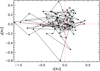 |
Fig. A.1. Photocentre position computed from RHD simulation st26gm07n001 in Table 1 in the Gaia G band filter. The different snapshots are connected by the line segments; the total time covered is reported in the Table. The dashed lines intersect at the position of the geometrical centre of the images. |
All Tables
All Figures
|
Fig. 1. Example of the squared root intensity maps (the range is |
| In the text | |
|
Fig. 2. Left panel: luminosity against the parallax error of the observations (σϖ, circle symbol in black) and the standard deviation of the photocentre displacement for the RHD simulations of Table 1 (σP, star symbol in red). Central panel: σP against the surface gravity for the RHD simulations. Right panel: σP against the logarithm of the period. |
| In the text | |
|
Fig. A.1. Photocentre position computed from RHD simulation st26gm07n001 in Table 1 in the Gaia G band filter. The different snapshots are connected by the line segments; the total time covered is reported in the Table. The dashed lines intersect at the position of the geometrical centre of the images. |
| In the text | |
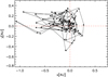 |
Fig. A.2. As in Fig. A.1 but for RHD simulation st26gm07n002 in Table 1. |
| In the text | |
 |
Fig. A.3. As in Fig. A.1 but for RHD simulation st27gm06n001 in Table 1. |
| In the text | |
 |
Fig. A.4. As in Fig. A.1 but for RHD simulation st28gm05n001 in Table 1. |
| In the text | |
 |
Fig. A.5. As in Fig. A.1 but for RHD simulation st28gm05n002 in Table 1. |
| In the text | |
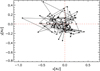 |
Fig. A.6. As in Fig. A.1 but for RHD simulation st28gm06n26 in Table 1. |
| In the text | |
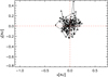 |
Fig. A.7. As in Fig. A.1 but for RHD simulation st29gm04n001 in Table 1. |
| In the text | |
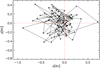 |
Fig. A.8. As in Fig. A.1 but for RHD simulation st29gm06n001 in Table 1. |
| In the text | |
Current usage metrics show cumulative count of Article Views (full-text article views including HTML views, PDF and ePub downloads, according to the available data) and Abstracts Views on Vision4Press platform.
Data correspond to usage on the plateform after 2015. The current usage metrics is available 48-96 hours after online publication and is updated daily on week days.
Initial download of the metrics may take a while.