| Issue |
A&A
Volume 690, October 2024
|
|
|---|---|---|
| Article Number | A31 | |
| Number of page(s) | 17 | |
| Section | The Sun and the Heliosphere | |
| DOI | https://doi.org/10.1051/0004-6361/202449836 | |
| Published online | 27 September 2024 | |
Charge sign dependence of recurrent Forbush decreases in 2016–2017
Christian-Albrechts-Universität zu Kiel, Leibnizstr. 11, 24118 Kiel, Germany
Received:
1
March
2024
Accepted:
28
June
2024
Abstract
Context. This study investigates the periodicities of galactic cosmic ray flux attributed to corotating interaction regions (CIRs) using Alpha Magnetic Spectrometer (AMS-02) data from late 2016 to early 2017.
Aims. We determine the rigidity dependence of recurrent Forbush decrease (RFD) amplitudes induced by CIRs for different particles with a focus on charge sign.
Methods. We carried out a frequency analysis using a Lomb-Scargle algorithm and superposed epoch analysis for all particles. For protons and helium, we compared the results with a single Forbush decrease (FD) analysis.
Results. Our results reveal that the rigidity dependence of proton amplitudes attributed to the northern coronal hole is in qualitative agreement with previous findings. In contrast, the amplitudes attributed to the southern coronal hole show no rigidity dependence. Furthermore, the amplitude of the helium modulation exceeds that of protons, in line with the observation for long-term modulation. For positrons, statistical limitations stand in the way of any definitive conclusions. In comparison to the positively charged particles, the modulation behavior of electrons reveals a different pattern.
Key words: Sun: heliosphere / Sun: magnetic fields / Sun: rotation / solar wind
Corresponding author; This email address is being protected from spambots. You need JavaScript enabled to view it. .
© The Authors 2024
 Open Access article, published by EDP Sciences, under the terms of the Creative Commons Attribution License (https://creativecommons.org/licenses/by/4.0), which permits unrestricted use, distribution, and reproduction in any medium, provided the original work is properly cited.
This article is published in open access under the Subscribe to Open model. This email address is being protected from spambots. You need JavaScript enabled to view it. to support open access publication.
1. Introduction
Galactic cosmic rays (GCRs) that propagate in the heliosphere are affected by solar activity. They are scattered at magnetic field irregularities, undergo convection and energy exchange in the expanding solar wind, and are exposed to gradient and curvature drifts in the large-scale heliospheric magnetic field (see for example Potgieter 2013, and references therein). The modulation of galactic cosmic rays (GCRs) occurs on different time scales from those corresponding to the solar cycle of 11 and 22 years down to variations of a few days (see e.g., Heber & Potgieter 2006; Aguilar et al. 2023a, and references therein).
The short-term modulation of the GCR flux due to heliospheric disturbances were first observed by Forbush (1937) and Hess & Demmelmair (1937), now referred to as Forbush decreases (FDs). There are two types of FDs. While the first one is associated with transient interplanetary disturbances caused by the interplanetary counterpart of a coronal mass ejection (ICME), as discussed in Cane (2000), the second type is of recurrent nature and has periodicities associated with the rotation period of the Sun of 27 days and their harmonics (see for example Richardson 2004, and references therein). The classical paradigm of recurrent FDs is summarized in Dumbović et al. (2022).
When fast solar wind originates from coronal holes (CHs), it interacts with the ambient slow solar wind leading to the creation of stream interaction regions (SIRs). As CHs are rather long-lived structures, SIRs may persist for several solar rotations corotating with the Sun; therefore, they are referred to as CIRs. The interaction forms a region of compressed plasma around the leading edge of the stream interface (i.e., increased total magnetic field and density), which is followed by a region of high temperature and flow speed (see for example Gosling & Pizzo 1999; Jian et al. 2006; Richardson 2018, and references therein). Recently Kopp et al. (2017) and Guo & Florinski (2016) modeled the interaction of GCRs with the CIR structures numerically. They utilized a magnetohydrodynamic (MHD) code to describe the background plasma leading to the environment in which the propagation of GCRs is described by the particle transport equation (PTE) derived by Parker (1965). This can be solved by utilizing the ansatz of stochastical differential equation (for details see Kopp et al. 2017, and references therein). An analytical approximation of this computations neglecting drift effects was derived by Vršnak et al. (2022) and successfully compared to single detector count rate measurements (see for example Kühl et al. 2020, and references therein) by the Electron Proton Helium INstrument (EPHIN) aboard the Solar and Heliospheric Observatory (SOHO). They conclude that the convection-diffusion GCR propagation hypothesis describes the observations of a long-lived recurrent FDs period in 2007–2008 well. The same period was investigated by Modzelewska et al. (2020), utilizing measurements from Payload for Antimatter Matter Exploration and Light-nuclei Astrophysics (PAMELA) (Adriani et al. 2014), EPHIN (Müller-Mellin et al. 1995), ARINA (Bakaldin et al. 2007), and Solar Terrestrial Relations Observatory (STEREO) High Energy Telescope (HET) (von Rosenvinge et al. 2008). Another study was performed by Paizis et al. (1999) for an extended CIR period from mid 1992 to September 1994 using the Ulysses Kiel Electron Telescope (KET) measurements. Both determined the amplitude of the recurrent modulation and found that for rigidities above 1 GV the rigidity dependence can be approximated by a power-law shape. The studies are in good agreement, indicating that for both magnetic epochs, drifts are of minor importance when attempting to explain the recurrent FDs.
However, up to the publication of the daily averaged fluxes of electrons by Aguilar et al. (2023a), no data existed that allowed to study recurrent FDs of electrons and protons at the same time. Aguilar et al. (2023a) show that electrons and protons have different long-term time profiles, which can be explained by drift effects (Potgieter 2013). In order to investigate this charge sign dependence on shorter time scales, we analyzed Alpha Magnet Spectromenter (AMS)-02 measurements from a period of five solar rotations in 2016 and 2017. This period was selected because there are two stable CH extending beyond the equator, which offers a great opportunity to study CIRs.
2. Instrumentation
The Alpha Magnet Spectromenter (AMS)-02, described in detail in Aguilar et al. (2021a), Kounine (2012), Ting (2013), Bertucci (2012), Incagli & AMS Collaboration (2010), and Battiston (2008), provides GCR measurements of different species at different rigidities. It is a magnetic spectrometer mounted on the International Space Station (ISS) that has been measuring since 2011. In this study, the AMS-02 data are linked to solar wind plasma data obtained by the Magnetometer (MAG) and Solar Wind Electron, Proton, and Alpha Monitor (SWEPAM) of the Advanced Composition Explorer (ACE, see Smith et al. 1998 and McComas et al. 1998, respectively), located at L1. Furthermore, data from the Electron Proton Helium INstrument (EPHIN) are utilized. EPHIN is part of Comprehensive Suprathermal and Energetic Particle Analyzer (COSTEP) onboard SOHO (Müller-Mellin et al. 1995) and is also located at L1.
Extreme ultraviolet (EUV) synoptic maps of the Sun have been constructed by Hamada et al. (2020). They are based on the Atmospheric Imaging Assembly (AIA), a four-telescope array operating primarily in the EUV, on board NASA’s Solar Dynamics Observatory (SDO), as described in Lemen et al. (2012).
3. Observation
The time period considered for this work extends from August 26, 2016 to January 10, 2017, which corresponds to Carrington rotation numbers 2181.0 to 2185.0.
3.1. Remote observation
Two persisting CHs characterize the entire period. This is illustrated in Fig. 1, where the upper panel displays EUV synoptic maps derived from AIA. Through analysis of the full-disk images, two recurring CHs can be discerned by their darker shades: one located in the southern hemisphere and the other in the northern hemisphere of the Sun. Both CHs can be attributed to different magnetic polarity as shown by the synoptic coronal hole maps from the Global Oscillation Network Group (GONG) given in the second panel. The GONG maps are based on the Potential-Field Source-Surface Model (PFSSM) and can be obtained online1. The source surface is fixed at 2.5 R where R is the radius of the Sun. All field lines reaching r = 2.5 R are open by assumption. The magnetic polarity of the open field lines referred to as coronal holes is represented by green (positive polarity) and red (negative polarity). The blue lines correspond to the highest closed field lines, with vanishing radial component just below 2.5 solar radii. The black solid line represents the neutral line and the black dashed line corresponds to the heliographic latitude of the Earth’s trajectory. We note that both CHs extend over the dashed black line in Fig. 1 for all Carrington rotations, leading to the expectation that the fast solar wind originating from these CHs will reach Earth.
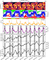 |
Fig. 1. Comparison of remote sensing observation with the in situ data for Carrington rotation 2181.0 to 2185.0, from top to bottom: (1) EUV synoptic maps based on SDO/AIA full-disk images at a wavelength of 193 Å. (2) GONG maps, where positive and negative magnetic polarity is denoted by green and red color, respectively. (3) Hourly Advanced Composition Explorer (ACE) magnetic field magnitude and local polarity. (4) Hourly solar wind speed measured by ACE/SWEPAM. (5) Hourly count rate of EPHIN single detector counter of scintillator anticoincidence G0. (6) Daily AMS proton flux with a rigidity of 1.00–1.16 GV. (7) Daily AMS proton flux with a rigidity of 5.37–5.90 GV. Note that the remote sensing maps (panels 1 and 2) have been mirrored in order to have the time running from left to right and the in situ data (panels 3 to 7) are backmapped to 2.5 solar radii. The grey areas mark the peaks of the solar wind speed ± 2 days. We note that EPHIN and AMS-02 flux is anticorrelated to solar wind speed. |
3.2. Comparison of remote observation with in situ measurements
In situ data obtained close to Earth need to be backmapped to their coronal source point to be compared to remote observations. We backmapped the data to the source surface of 2.5 solar radii to make them comparable to the GONG maps. The effects of the backmapping of solar wind is illustrated in Fig. 2. The left panel sketches the configuration to derive the corresponding equation:
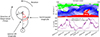 |
Fig. 2. Illustration for the method of backmapping. Left: View of the sun from the north (N). The longitude of the spacecraft (S) is marked by A. When the emitted solar wind is detected by the spacecraft, the sun has continued to rotate by the angle ΔΦ leading to the backmapped longitude marked by B. Then, r and r0 are the heliocentric distance of the spacecraft and of the source surface at 2.5 solar radii, respectively. Right: GONG-map of carrington rotation 2184.0 (top; note: the map has been mirrored in order to have the time running from left to right). The in situ solar wind speed and magnetic polarity as measured at 1 AU and the backmapped data according to Eq. (1) (bottom). It is evident that the high speed streams of the backmapped data can be associated more accurately with the respective CH. |
If T is the synodic rotation period of the Sun, Vsw the measured solar wind speed, r and r0 the heliocentric distance of the spacecraft and of the source surface at 2.5 solar radii, respectively, the angle Δϕ in Fig. 2 can be calculated via
 (1)
(1)
when assuming constant radial solar wind speed. By knowing the angle Δϕ, we can calculate the travel time of the solar wind speed by
 (2)
(2)
Each data point is then shifted back by the travel time, as illustrated in Fig. 2 (right). For more details, we refer, for instance, to Schwenn & Marsch (1990) and Nolte & Roelof (1973).
Figure 1 compares the remote sensing with backmapped in situ data. The third panel shows the structures of the interplanetary magnetic field (IMF)’s amplitude measured by the Magnetometer (MAG) of ACE. In-situ magnetic polarity was calculated via the spatial components of the magnetic field also measured by MAG. It is given in the colored band and can be attributed to the according polarity of the CH. The solar wind velocity as measured by the SWEPAM on ACE is shown in panel 4. We can observe fast solar wind streams originating from each CH. The GCR intensity is anticorrelated to fast solar wind streams, as shown, for example, by the EPHIN count rate in panel 5. In panels 6 and 7, the AMS-02 proton fluxes at different rigidities are shown. We notice the difference in modulation at the two rigidities.
In the following the amplitude of the GCR decreases attributed to the CHs will be studied systematically utilizing AMS-02 data for protons (Aguilar et al. 2021b), helium (Aguilar et al. 2022), electrons (Aguilar et al. 2023a), and positrons (Aguilar et al. 2023b).
4. Data analysis
We analyzed the data using two different approaches. In the first, we examined the flux decrease as a function of rigidity. Therefor the decreases are averaged for helium and protons (statistical analysis). Due to the poor statistics of electrons and (especially) positrons, we also applied a superposed epoch analysis. In the second approach, we use an implementation of a Lomb-Scargle (Lomb 1976 and Scargle 1982) algorithm to detect periodically occurring structures. For the confidence evaluation, the background of the data was modeled with red noise.
4.1. Statistical analysis
In this method, we define FDs based on specific time periods and determine their amplitude. The investigated period of five solar rotations is divided into slightly overlapping 14 day periods. Each of those periods, following Fig. 3, are assumed to have been influenced by exactly one CIR. In those periods, we define the amplitude of the FD as follows: all local minima and maxima are being determined and the differences of all possible maximum-minimum pairings are computed. All pairings that are increases, meaning that the maximum follows the minimum, are then being excluded. The largest remaining difference is then defined as the amplitude of the FD of the corresponding period. These amplitudes are then assigned to one of two categories: they are influenced by a CIR originating either from the northern (green) or the southern (red) CH. Figure 3 shows the amplitudes for protons and their categorization at two different rigidities. While at high rigidity the amplitudes are almost independent of the CH polarity, they are about four times lower for the southern CH at low rigidity.
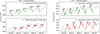 |
Fig. 3. Daily averaged AMS-02 1.00–1.16 GV (left) and 5.37–5.90 GV (right) proton flux vs. time. Colored periods are assumed to contain a FD caused by a CIR originating either from the northern (green) or the southern (red) CH. The numbers given in those plots correspond to the amplitude of the decrease, given in units of the flux. |
In order to investigate this effect in detail, this procedure is repeated for rigidities up to 20 GV. The amplitudes of those FDs are averaged and normalized to the average flux of the analyzed time span. The rigidity dependence of the amplitudes caused by the northern CH (green data points) was determined by fitting a power law:
 (3)
(3)
to the data below 10 GV, shown in Fig. 4 and discussed in Sect. 5. This range was chosen in accordance with predictions from models (Luo et al. 2024).
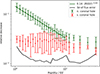 |
Fig. 4. Relative amplitudes of FDs versus rigidity. The color coding shows the polarity of the CH responsible for the FD, same as in Fig. 3. The relative amplitudes caused by the northern CH has been fitted by a power law (Eq. (3)) in the rigidity range from 1–10 GV. The black lines show three times the average error of the fluxes in the analyzed time period of five solar rotations. |
4.2. Superposed epoch analysis
The rigidity dependence of the northern CH has also been determined by a superposed epoch analysis for all particles. The main advantage of this method is the reduction of statistical fluctuation, therefore, it is not expected to give different results for protons or helium, but it is necessary to get meaningful results for electrons and positrons. For every single green period in Fig. 3, the day of maximum flux has been determined for each rigidity. The most probable day of all rigidities serves as the reference point for time and flux normalization for every period. Thus, the reference points are based on the most probable day of maximum flux for protons and are considered to be the same for every particle type and rigidity. From this maximum point, one rotation is being defined to start three days before it and end ten days after it. This leads to five rotations with similar behavior as shown in Fig. 5 (left panel) for 1.0–1.16 GV protons.
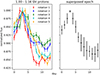 |
Fig. 5. Normalized AMS-02 1.00–1.16 GV proton flux vs. day (left). Colors indicate different time periods of five analyzed solar rotations. The periods shown are similar to the green periods in Fig. 3. Averaged normalized flux for every day (right). |
Those rotations have then been averaged, leading to the result shown on the right panel, called a superposed epoch. The amplitude has then been determined for those superposed epochs for every rigidity, shown by the light green points in Fig. 6, also discussed in Sect. 5.
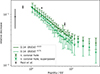 |
Fig. 6. Relative amplitudes of FDs vs. rigidity. Dark green displays the averaging of the five FDs while light green is based on the superposed epoch analysis. The dark green points are identical to Fig. 4 (same as in Fig. 3). The relative amplitudes have been fitted by a power law in the rigidity range from 1–10 GV for both methods. For comparison, the data from Paizis et al. (1999) are shown in black. |
4.3. Analysis via Lomb-Scargle
In this method, we use the Lomb-Scargle algorithm after Lomb (1976) and Scargle (1982) to analyze occuring periodicities. The algorithm is particularly suitable for our analysis since it performs robustly in the presence of data gaps. It fits a sinusoidal model to the data at certain frequencies, f, and compares the resulting residuals to residuals of a constant reference fit. The normalized power is defined as:
 (4)
(4)
where χ2(f) symbolizes the residuals of the sinusoidal fit at frequency f and χref2 the residuals of a constant reference model. With that, larger power reflects a better fit. The un-normalized power is defined as:
![Mathematical equation: $$ \begin{aligned} P_{\text{unnorm}} = \frac{1}{2}[\chi ^2_{\text{ref}} - \chi ^2(f)] \end{aligned} $$](/articles/aa/full_html/2024/10/aa49836-24/aa49836-24-eq5.gif) (5)
(5)
This normalization is constructed to be comparable to the standard Fourier power spectral density (psd) (VanderPlas 2018). The amplitude C of the fit to the periodic signal can be calculated as follows:
 (6)
(6)
where N is the number of data points, ti the ith time point and ϕ the phase shift. The above equation reduces to
 (7)
(7)
when considering evenly sampled data and time spans that correspond to integer multiples of half of the investigated period.
To eliminate the influence of the solar cycle induced long term trend, the data have been detrended via a running mean of half a year window. To determine the significance of detected signals, a model for the background is needed. We assumed the background of the AMS-02 signal to be red noise, which is defined as follows:
 (8)
(8)
where an is the nth value, an − 1 is the (n − 1)th value, α is the lag 1 autocorreleation coefficient and z is a normally distributed random number.
Figure B.1 shows the detrended proton flux at 1 GV. The shaded area marks the observation period. The corresponding auto correlations are given in the lower panel. Then, α is calculated as the weighted average of the two AMS-02 signal auto correlation coefficients. Data gaps are ignored and the auto correlation is estimated treating the non-missing as contiguous time series. This leads to a slight underestimation of α (below few percents for all particles and rigidities). The associated background signal was calculated according to Eq. (8). This signal is given in the upper panel of Fig. B.1 as red line. For all three signals, we observe an exponential decay of the auto correlation, which corresponds to the definition of red noise. The auto correlation coefficients α for all rigidities and particles are listed in Table B.1.
To determine the significance of the normalized power, we compute the probability density function (PDF) as follows: 100 000 randomly generated red noise signals with the corresponding α are created and the periodograms of each. The PDF is computed as the normalized histogram. Figure B.2 (left) shows the PDF to obtain a certain normalized power at a given period for protons around 1 GV. The dotted red line marks the uncorrected confidence level CLuncorr of 95%. 5% of all power values exceed the CLuncorr at a given period. Subsequently, we increased the CLuncorr stepwise. At each step, we determined the percentage of periodograms that did not exceed the CLuncorr at any period. We call this percentage the corrected confidence level CLcorr. On the right of Fig. B.2 the relation between CLcorr and CLuncorr is shown. The dotted and dashed red lines mark a CLcorr of 95% that corresponds to a CLuncorr of 99.83% and is only exceeded by 5% of all periodograms at any period. This corrected confidence level is also given on the left of Fig. B.2. With this method, the uncorrected confidence level is corrected for the number of investigated periods as VanderPlas (2018) does for white noise. An analytical approach for this correction for red noise is given in Vaughan (2005).
The resulting periodogram for protons is shown in Fig. 7. The left side shows the relative proton flux for three rigidity bins. The lower panel gives the resulting normalized power according to Eq. (4). The dashed lines mark the respective corrected confidence levels and the dotted lines the uncorrected ones. The right side of Fig. 7 shows the normalized power for protons for all rigidity bins. The height at which the normalized power becomes significant is marked by the dashed and dotted line for a corrected and uncorrected confidence level, respectively. Similarly to Aguilar et al. (2021b), we see a strong normalized power at periodicities around 13.5 and 27 days for protons. Considering the corrected confidence level CLuncorr, the normalized power around 13.5 days is significant below approximately 30 GV and periodicities around 27 days show significant normalized power for all rigidities below 3 GV.
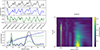 |
Fig. 7. Relative proton flux for three rigidity bins (top three columns on the left). The lower-left panel gives the resulting normalized power according to Eq. (4). The dashed lines mark the respective corrected confidence levels and the dotted lines the uncorrected ones. Right: Color coding gives the normalized power for protons for all rigidity bins. Again, the dashed and dotted line mark the height at which the normalized power becomes significant for the corrected and uncorrected confidence level, respectively. |
Below, we construct the null hypotheses that serve as the foundation for testing the significance of normalized power:
-
null hypothesis 1: There are no significant periodicities in the signal at any period. This hypothesis is tested with the corrected confidence level. Protons are tested against the corrected confidence level CLcorr. In Fig. 7 we see that protons show significant normalized power with a CLcorr of 95 % at about 13.5 and 27 days.
-
null hypothesis 2: There are no significant periodicities in the signal at a given period. This hypothesis is tested with the uncorrected confidence level. Since protons are the most abundant species and have been tested against the corrected confidence level to have a significant normalized power at 27 and 13.5 days, the helium, positrons, and electrons are only tested for significance at these periods. This means that we use the uncorrected confidence level, CLuncorr, as we are only interested in whether the particles show significant normalized power at 27 or 13.5 days.
For comparison, both the uncorrected and the corrected confidence level are plotted in all periodograms. The results are given in Fig. 7 for protons and in Fig. C.1 for helium, positrons, and electrons and are discussed in Sect. 5.
To investigate the rigidity dependence of the amplitudes of the FDs, the amplitude of the sinusoidal fit according to Eq. (6) at 13.5 and 27 days is determined. This was accomplished by identifying the height of the peaks of the unnormalized power (Eq. (5)) within the range of 12.5 to 14.5 days and of 25 to 29 days for the 13.5 and 27 day periodicity, respectively. Figure 8 shows the amplitudes versus rigidity for protons. The errorbars denote the amplitude error of the sinusoidal fitted by the Lomb-Scargle algorithm. This figure is also discussed in Sect. 5.
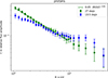 |
Fig. 8. Amplitude of the Lomb-Scargle fit (Eq. (6)) vs. rigidity for a periodicity of 27 and 13.5 days for protons. The solid lines represent a power-law fit (Eq. (3)) below 10 GV to the data. |
5. Results
5.1. Statistical analysis
The results from the statistical analysis are shown in Fig. 4 for protons together with three times the average flux uncertainty. It can be seen that the amplitudes of the FDs are larger than what would be expected from statistical fluctuation below 40 GV. The FDs caused by the northern CH clearly show a different rigidity dependence; namely, a power law with negative power. For helium and protons, the power is constant below 10 GV. In contrast, the FDs caused by the southern CH reveal no rigidity dependence. For comparison, the rigidity dependence of the single rotations including the power-law fits to the FDs caused by the northern CH are given in Fig. A.1. We see that each single rotation shows a slightly different course for the southern coronal hole. In particular, the second period differs from the averaged constant rigidity dependence (as shown in Fig. 4). However, the statistics for one single period is quite bad. For the northern coronal hole, the rigidity dependence shows overall the same pattern as the averaged amplitudes. The power-law fits to the averaged amplitudes of the northern coronal hole for helium, positrons, and electrons are given in Fig. A.2 (in dark green).
5.2. Superposed epoch analysis
The superposed epoch analysis is only applied for the northern CH to improve precision of the power law fit. This is particularly relevant for particles with lower statistics such as electrons and positrons, as the averaging of several rotations leads to a significant reduction of statistical fluctuation. The amplitudes of the southern coronal hole remain constant over rigidity as the statistical analysis has shown. Therefore, we did not fit a power law to the amplitudes, nor did we apply the superposed epoch analysis for the southern coronal hole.
The results of the superposed epoch analysis are shown by the light green points in Fig. 6 for protons and in Fig. A.2 for helium, electrons, and positrons. The points in dark green of Fig. 6 are identical to the ones in Fig. 4 and the black points are from Paizis et al. (1999).
The fit parameters from Eq. (3) of the superposed epoch analysis are given in Table 1 for rigidities below 10 GV. We note that for this method, all the fit parameters are within their respective errors for positively charged particles; however, for positrons, the errors are too large to draw definite conclusions. In the case of helium and protons, the error has probably been overestimated, as the fitted function is within every single error bar. Furthermore, as can be seen in Tables A.1 and A.2, helium has systematically larger decreases below 4 GV. As a result, it is still reasonable to assume that helium is being modulated slightly more than protons by CIRs at low rigidities. This is in qualitative agreement with the findings of Aguilar et al. (2022) for long term modulation. On the other hand, electrons show significantly weaker periodic behavior than particles of positive charge.
5.3. Analysis via Lomb-Scargle
From the Lomb-Scargle analysis as shown in Fig. 7, we see that protons show significant normalized power at 27 days below 3 GV and between 4.88–5.37 GV and at 13.5 days below 30 GV considering the corrected confidence level CLcorr. In Fig. C.2, we can see for protons, that the 13.5 day normalized power increases up to approximately 20 GV, whereas the 27 day power decreases. For helium, positrons, and electrons, we only considered the peaks around 13.5 and 27 days and the uncorrected confidence level CLuncorr (see Sect. 4.3) for significance evaluation. Helium shows significant periodicities at 27 days for all rigidity bins below 5.37 GV. Between 5.37 and 13 GV, we could observe three significant peaks. At 13.5 days the peaks of the normalized power stay significant below 33.5 GV. Positrons show significant peaks around 27 days below 2.15 GV. We did not observe significant peaks at 13.5 days; however, below 5.9 GV we observed significant normalized power around 14 to 14.5 days and for the highest rigidity bin, there are two peaks around 12 and 15 days. Electrons show a different pattern than the positively charged particles. We did not observe significant peaks at 27 and 13.5 days.
The rigidity analysis of the amplitudes obtained from the Lomb-Scargle algorithm is shown in Fig. 8 for protons and in Fig. C.3 for helium, positrons, and electrons. We observed that the 27 day amplitude decreases faster with rigidity than the 13.5 day amplitude for particles with positive charge. For the fitting of the power law, we only considered the 27 day periodicity, since this periodicity is mainly driven by the northern CH. We note that for this analysis, the amplitudes of the fits were considered, regardless of whether the corresponding peaks are significant or not. Again, the power law was fitted from 1 to 10 GV. The parameters obtained by the fitting are listed in Table 1. We note that the amplitudes, A, are in agreement for positively charged particles. While the electron amplitude disagrees with about 1σ for positrons, it disagrees with about 3σ for protons. For the spectral index, γ, we note that the precision available for the electrons and positrons is insufficient to draw accurate conclusions.
The amplitudes obtained from Lomb-Scargle and superposed epoch analysis may not be directly comparable, but they still show a similar overall pattern. We do find a good agreement of γ within the respective uncertainty for all particles. In particular, the Lomb-Scargle analysis confirms the findings of the superposed epoch analysis that helium is modulated more than protons.
6. Discussion and conclusions
The FDs caused by the northern CH and the 27 day periodicity are largely in agreement with expectations from earlier measurements and theory. In accordance with Modzelewska et al. (2020) and Paizis et al. (1999), we were able to show that the amplitudes of FDs decreases with rigidity and has a power-law shape. Modzelewska et al. (2020) found a power-law index of γ = −0.51 ± 0.11 for PAMELA protons above 1 GV in 2007 to 2008; this result is slightly lower than our findings. However, the results are not directly comparable, as 2007 to 2008 corresponds to a negative solar magnetic epoch and the time period analyzed in this work corresponds to a positive solar magnetic epoch. Luo et al. (2024) modeled the effects of CIRs on GCR protons by integrating a MHD model of the CIR structure into a Parker transport model. For 1 to 10 GV protons, they found a power-law index of γ = −0.438 in agreement to Modzelewska et al. (2020) and also lower than our findings.
As Aguilar et al. (2022) pointed out, helium appears to be modulated more than protons for long term modulation, which agrees with our finding for modulation caused by CIRs. Heber et al. (2002, 2003); Heber et al. (2009) demonstrated the impact of the solar cycle on GCR modulation, showing a dependence on the charge sign, attributed to drift effects. Our results may also suggest a charge sign-dependent modulation pattern, since the modulation of electrons caused by the CIRs differs from that of protons, helium, and positrons. Fig. 2 in Aguilar et al. (2023a) indicate that this effect may be due to the magnetic polarity of the solar cycle. There, it appears that the modulation behavior of electrons and protons reverses when considering the opposite solar magnetic epoch.
Unexpectedly, the amplitudes of the FDs caused by the southern CH, show no dependence from rigidity. This finding cannot be reproduced directly by the Lomb-Scargle algorithm. According to Parker (1965), four processes influence galactic cosmic rays in the heliosphere: diffusion, drifts, convection, and energy change. However, Dumbović et al. (2011) identified that convection and energy change are not significant for FDs. To analyze the influence of diffusion and drifts, it is planned to extend this analysis to a larger sample of CIRs. We note that, if two FDs are
-
of a similar amplitude
-
recurrent
-
caused by two different CHs which are separated by roughly 180 degrees
a frequency analysis will result in a strong 13.5 day power. If the amplitudes of the two FDs are significantly different, the result will be a strong 27 day power. This accounts for the decline in 27 day power and the concurrent rise in 13.5 day power with rigidity during the analyzed period, which reinforces the very different rigidity dependence of the two CHs.
In conclusion, we determined the rigidity dependence for CIR modulated protons, helium, positrons, and electrons. The rigidity dependence of positively charged particles influenced by the northern coronal hole analyzed via the superposed epoch analysis and the Lomb-Scargle algorithm is generally in agreement with other studies. We demonstrate that electrons behave differently than positively charged particles, which could possibly be attributed to magnetic epoch effects. One aspect that is particularly surprising, however, is the modulation behavior caused by the southern coronal hole. Here, the amplitudes of the FD are independent of the rigidity. To gain more insights into these processes, it is worthwhile investigating the plasma and magnetic field properties of the CIRs, the modulation of Jovian electrons, and the acceleration of low-energy ions and electrons.
Acknowledgments
The SOHO/EPHIN and AMS 02 are supported under Grant 50 OC 2302 and 50OO1804 by the German Bundesministerium für Wirtschaft through the Deutsches Zentrum für Luft- und Raumfahrt (DLR). We are grateful for important physics discussions with Ilya Usoskin, Rami Vainio, Vladimir Mikhailov, Cristina Consolandi, Claudio Corti and Yi Jia.
References
- Adriani, O., Barbarino, G. C., Bazilevskaya, G. A., et al. 2014, Phys. Rep., 544, 323 [Google Scholar]
- Aguilar, M., Ali Cavasonza, L., Ambrosi, G., et al. 2021a, Phys. Rep., 894, 1 [NASA ADS] [CrossRef] [Google Scholar]
- Aguilar, M., Cavasonza, L. A., Ambrosi, G., et al. 2021b, Phys. Rev. Lett., 127, 271102 [NASA ADS] [CrossRef] [Google Scholar]
- Aguilar, M., Cavasonza, L. A., Ambrosi, G., et al. 2022, Phys. Rev. Lett., 128, 231102 [NASA ADS] [CrossRef] [Google Scholar]
- Aguilar, M., Cavasonza, L. A., Ambrosi, G., et al. 2023a, Phys. Rev. Lett., 130, 161001 [Google Scholar]
- Aguilar, M., Ambrosi, G., Anderson, H., et al. 2023b, Phys. Rev. Lett., 131, 161001 [NASA ADS] [CrossRef] [Google Scholar]
- Bakaldin, A. V., Batishchev, A. G., Voronov, S. A., et al. 2007, Cosmic Res., 45, 445 [NASA ADS] [CrossRef] [Google Scholar]
- Battiston, R. 2008, Nucl. Instrum. Methods Phys. Res. Sect. A, 588, 227 [CrossRef] [Google Scholar]
- Bertucci, B. 2012, PoS, EPS-HEP2011, 067 [Google Scholar]
- Cane, H. V. 2000, Space Sci. Rev., 93, 55 [NASA ADS] [CrossRef] [Google Scholar]
- Dumbović, M., Vršnak, B., Čalogović, J., & Karlica, M. 2011, A&A, 531, A91 [NASA ADS] [CrossRef] [EDP Sciences] [Google Scholar]
- Dumbović, M., Vršnak, B., Temmer, M., Heber, B., & Kühl, P. 2022, A&A, 658, A187 [NASA ADS] [CrossRef] [EDP Sciences] [Google Scholar]
- Forbush, S. E. 1937, Phys. Rev., 51, 1108 [NASA ADS] [CrossRef] [Google Scholar]
- Gosling, J. T., & Pizzo, V. J. 1999, Space Sci. Rev., 89, 21 [NASA ADS] [CrossRef] [Google Scholar]
- Guo, X., & Florinski, V. 2016, ApJ, 826, 65 [NASA ADS] [CrossRef] [Google Scholar]
- Hamada, A., Asikainen, T., & Mursula, K. 2020, Sol. Phys., 295, 2 [NASA ADS] [CrossRef] [Google Scholar]
- Heber, B., & Potgieter, M. S. 2006, Space Sci. Rev., 127, 117 [Google Scholar]
- Heber, B., Wibberenz, G., Potgieter, M. S., et al. 2002, J. Geophys. Res. Space Phys., 107, A10 [CrossRef] [Google Scholar]
- Heber, B., Clem, J. M., Müller-Mellin, R., et al. 2003, Geophys. Res. Lett., 30, 19 [CrossRef] [Google Scholar]
- Heber, B., Kopp, A., Gieseler, J., et al. 2009, ApJ, 699, 1956 [Google Scholar]
- Hess, V. F., & Demmelmair, A. 1937, Nature, 140, 316 [NASA ADS] [CrossRef] [Google Scholar]
- Incagli, M., & AMS Collaboration 2010, AIP Conf. Proc., 1223, 43 [CrossRef] [Google Scholar]
- Jian, L., Russell, C. T., Luhmann, J. G., & Skoug, R. M. 2006, Sol. Phys., 239, 337 [NASA ADS] [CrossRef] [Google Scholar]
- Kopp, A., Wiengarten, T., Fichtner, H., et al. 2017, ApJ, 837, 37 [NASA ADS] [CrossRef] [Google Scholar]
- Kounine, A. 2012, Int. J. Modern Phys. E, 21, 1230005 [NASA ADS] [CrossRef] [Google Scholar]
- Kühl, P., Heber, B., Gómez-Herrero, R., et al. 2020, J. Space Weather Space Climate, 10, 53 [CrossRef] [EDP Sciences] [Google Scholar]
- Lemen, J. R., Title, A. M., Akin, D. J., et al. 2012, Sol. Phys., 275, 17 [Google Scholar]
- Lomb, N. R. 1976, Astrophys. Space Sci., 39, 447 [Google Scholar]
- Luo, X., Potgieter, M. S., Zhang, M., & Shen, F. 2024, ApJ, 961, 21 [NASA ADS] [CrossRef] [Google Scholar]
- McComas, D., Bame, S., Barker, P., et al. 1998, Space Sci. Rev., 86, 563 [Google Scholar]
- Modzelewska, R., Bazilevskaya, G. A., Boezio, M., et al. 2020, ApJ, 904, 3 [NASA ADS] [CrossRef] [Google Scholar]
- Müller-Mellin, R., Kunow, H., Fleißner, V., et al. 1995, Sol. Phys., 162, 483 [Google Scholar]
- Nolte, J. T., & Roelof, E. C. 1973, Sol. Phys., 33, 241 [NASA ADS] [CrossRef] [Google Scholar]
- Paizis, C., Heber, B., Ferrando, P., et al. 1999, J. Geophys. Res., 104, 28241 [CrossRef] [Google Scholar]
- Parker, E. N. 1965, Planet. Space Sci., 13, 9 [Google Scholar]
- Potgieter, M. S. 2013, Liv. Rev. Sol. Phys., 10, 3 [Google Scholar]
- Richardson, I. G. 2004, Space Sci. Rev., 111, 267 [Google Scholar]
- Richardson, I. G. 2018, Liv. Rev. Sol. Phys., 15, 1 [Google Scholar]
- Scargle, J. D. 1982, ApJ, 263, 835 [Google Scholar]
- Schwenn, R., & Marsch, E. 1990, Physics of the Inner Heliosphere I (Berlin Heidelberg: Springer) [CrossRef] [Google Scholar]
- Smith, C., L’Heureux, J., Ness, N., et al. 1998, Space Sci. Rev., 86, 613 [Google Scholar]
- Ting, S. 2013, Nucl. Phys. B, 12, 243 [Google Scholar]
- VanderPlas, J. T. 2018, ApJS, 236, 16 [Google Scholar]
- Vaughan, S. 2005, A&A, 431, 391 [NASA ADS] [CrossRef] [EDP Sciences] [Google Scholar]
- von Rosenvinge, T. T., Reames, D. V., Baker, R., et al. 2008, Space Sci. Rev., 136, 391 [Google Scholar]
- Vršnak, B., Dumbović, M., Heber, B., & Kirin, A. 2022, A&A, 658, A186 [NASA ADS] [CrossRef] [EDP Sciences] [Google Scholar]
Appendix A: Amplitudes of Forbush decreases
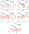 |
Fig. A.1. Relative proton amplitudes vs. rigidity for single solar rotations. The color coding shows the polarity of the CH responsible for the FD (green and red for positive and negative polarity, respectively). The relative amplitudes caused by the northern CH has been fitted by a power law (Eq. 3) in the rigidity range from 1-10 GV. The black lines show three times the average error of the fluxes in the analyzed time period of five solar rotations. |
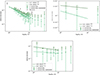 |
Fig. A.2. Relative amplitudes of FDs vs. rigidity for helium (upper left), positrons (upper light) and electrons (lower panel). Dark green is based on averaging the 5 FDs while light green is based on the superposed epoch analysis. The relative amplitudes have been fitted by a power law in the rigidity range from 1-10 GV for both methods. |
Amplitudes of Forbush decreases of protons.
Amplitudes of Forbush decreases of helium.
Amplitudes of Forbush decreases of positrons.
Amplitudes of Forbush decreases of electrons.
Appendix B: Confidence levels
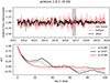 |
Fig. B.1. Detrended AMS-02 proton flux at 1 GV (black lines) and estimated background modeled by red noise (red line), shown at the top. The grey shaded area marks the analysis period of this work. Bottom panel: Auto correlation of the above time series. |
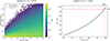 |
Fig. B.2. PDFs used to obtain a certain normalized power at a given period for 1 GV protons (left). The auto correlation coefficient for this figure is α = 0.89. The dotted red line marks the uncorrected confidence level CLuncorr of 95 %. Overall, 5 % of all power values exceed the CLuncorr at a given period . The dashed red line marks a CLuncorr of 99.83 %. This confidence level is only exceeded by 5 % of all periodograms at any period. Right: The relation between corrected and uncorrected CL is shown. The dotted and dashed red lines mark a CLuncorr of 95 %, which corresponds to a CLcorr of 99.83 %. |
Lag 1 autocorrelation coefficients, α, for all four particles.
Appendix C: Lomb-Scargle analysis
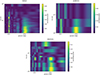 |
Fig. C.1. Lomb-Scargle analysis: periodograms for all helium, positrons, and electrons. The dashed and dotted line mark the height at which the normalized power becomes significant for a corrected and uncorrected confidence level of 95 %, respectively. |
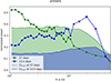 |
Fig. C.2. Normalized power at 27 and 13.5 days vs. rigidity for protons. The dashed line shows the height of the CLcorr of 95 % at 27 and 13.5 days, respectively. |
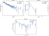 |
Fig. C.3. Amplitude of the Lomb-Scargle fit (Eq. 6) vs. rigidity for a periodicity of 27 and 13.5 days for helium positrons and electrons. The solid lines represent a power-law fit below 10 GV (Eq. 3) to the data. |
All Tables
All Figures
|
Fig. 1. Comparison of remote sensing observation with the in situ data for Carrington rotation 2181.0 to 2185.0, from top to bottom: (1) EUV synoptic maps based on SDO/AIA full-disk images at a wavelength of 193 Å. (2) GONG maps, where positive and negative magnetic polarity is denoted by green and red color, respectively. (3) Hourly Advanced Composition Explorer (ACE) magnetic field magnitude and local polarity. (4) Hourly solar wind speed measured by ACE/SWEPAM. (5) Hourly count rate of EPHIN single detector counter of scintillator anticoincidence G0. (6) Daily AMS proton flux with a rigidity of 1.00–1.16 GV. (7) Daily AMS proton flux with a rigidity of 5.37–5.90 GV. Note that the remote sensing maps (panels 1 and 2) have been mirrored in order to have the time running from left to right and the in situ data (panels 3 to 7) are backmapped to 2.5 solar radii. The grey areas mark the peaks of the solar wind speed ± 2 days. We note that EPHIN and AMS-02 flux is anticorrelated to solar wind speed. |
| In the text | |
|
Fig. 2. Illustration for the method of backmapping. Left: View of the sun from the north (N). The longitude of the spacecraft (S) is marked by A. When the emitted solar wind is detected by the spacecraft, the sun has continued to rotate by the angle ΔΦ leading to the backmapped longitude marked by B. Then, r and r0 are the heliocentric distance of the spacecraft and of the source surface at 2.5 solar radii, respectively. Right: GONG-map of carrington rotation 2184.0 (top; note: the map has been mirrored in order to have the time running from left to right). The in situ solar wind speed and magnetic polarity as measured at 1 AU and the backmapped data according to Eq. (1) (bottom). It is evident that the high speed streams of the backmapped data can be associated more accurately with the respective CH. |
| In the text | |
|
Fig. 3. Daily averaged AMS-02 1.00–1.16 GV (left) and 5.37–5.90 GV (right) proton flux vs. time. Colored periods are assumed to contain a FD caused by a CIR originating either from the northern (green) or the southern (red) CH. The numbers given in those plots correspond to the amplitude of the decrease, given in units of the flux. |
| In the text | |
|
Fig. 4. Relative amplitudes of FDs versus rigidity. The color coding shows the polarity of the CH responsible for the FD, same as in Fig. 3. The relative amplitudes caused by the northern CH has been fitted by a power law (Eq. (3)) in the rigidity range from 1–10 GV. The black lines show three times the average error of the fluxes in the analyzed time period of five solar rotations. |
| In the text | |
|
Fig. 5. Normalized AMS-02 1.00–1.16 GV proton flux vs. day (left). Colors indicate different time periods of five analyzed solar rotations. The periods shown are similar to the green periods in Fig. 3. Averaged normalized flux for every day (right). |
| In the text | |
|
Fig. 6. Relative amplitudes of FDs vs. rigidity. Dark green displays the averaging of the five FDs while light green is based on the superposed epoch analysis. The dark green points are identical to Fig. 4 (same as in Fig. 3). The relative amplitudes have been fitted by a power law in the rigidity range from 1–10 GV for both methods. For comparison, the data from Paizis et al. (1999) are shown in black. |
| In the text | |
|
Fig. 7. Relative proton flux for three rigidity bins (top three columns on the left). The lower-left panel gives the resulting normalized power according to Eq. (4). The dashed lines mark the respective corrected confidence levels and the dotted lines the uncorrected ones. Right: Color coding gives the normalized power for protons for all rigidity bins. Again, the dashed and dotted line mark the height at which the normalized power becomes significant for the corrected and uncorrected confidence level, respectively. |
| In the text | |
|
Fig. 8. Amplitude of the Lomb-Scargle fit (Eq. (6)) vs. rigidity for a periodicity of 27 and 13.5 days for protons. The solid lines represent a power-law fit (Eq. (3)) below 10 GV to the data. |
| In the text | |
|
Fig. A.1. Relative proton amplitudes vs. rigidity for single solar rotations. The color coding shows the polarity of the CH responsible for the FD (green and red for positive and negative polarity, respectively). The relative amplitudes caused by the northern CH has been fitted by a power law (Eq. 3) in the rigidity range from 1-10 GV. The black lines show three times the average error of the fluxes in the analyzed time period of five solar rotations. |
| In the text | |
|
Fig. A.2. Relative amplitudes of FDs vs. rigidity for helium (upper left), positrons (upper light) and electrons (lower panel). Dark green is based on averaging the 5 FDs while light green is based on the superposed epoch analysis. The relative amplitudes have been fitted by a power law in the rigidity range from 1-10 GV for both methods. |
| In the text | |
|
Fig. B.1. Detrended AMS-02 proton flux at 1 GV (black lines) and estimated background modeled by red noise (red line), shown at the top. The grey shaded area marks the analysis period of this work. Bottom panel: Auto correlation of the above time series. |
| In the text | |
|
Fig. B.2. PDFs used to obtain a certain normalized power at a given period for 1 GV protons (left). The auto correlation coefficient for this figure is α = 0.89. The dotted red line marks the uncorrected confidence level CLuncorr of 95 %. Overall, 5 % of all power values exceed the CLuncorr at a given period . The dashed red line marks a CLuncorr of 99.83 %. This confidence level is only exceeded by 5 % of all periodograms at any period. Right: The relation between corrected and uncorrected CL is shown. The dotted and dashed red lines mark a CLuncorr of 95 %, which corresponds to a CLcorr of 99.83 %. |
| In the text | |
|
Fig. C.1. Lomb-Scargle analysis: periodograms for all helium, positrons, and electrons. The dashed and dotted line mark the height at which the normalized power becomes significant for a corrected and uncorrected confidence level of 95 %, respectively. |
| In the text | |
|
Fig. C.2. Normalized power at 27 and 13.5 days vs. rigidity for protons. The dashed line shows the height of the CLcorr of 95 % at 27 and 13.5 days, respectively. |
| In the text | |
|
Fig. C.3. Amplitude of the Lomb-Scargle fit (Eq. 6) vs. rigidity for a periodicity of 27 and 13.5 days for helium positrons and electrons. The solid lines represent a power-law fit below 10 GV (Eq. 3) to the data. |
| In the text | |
Current usage metrics show cumulative count of Article Views (full-text article views including HTML views, PDF and ePub downloads, according to the available data) and Abstracts Views on Vision4Press platform.
Data correspond to usage on the plateform after 2015. The current usage metrics is available 48-96 hours after online publication and is updated daily on week days.
Initial download of the metrics may take a while.