| Issue |
A&A
Volume 694, February 2025
|
|
|---|---|---|
| Article Number | A197 | |
| Number of page(s) | 11 | |
| Section | The Sun and the Heliosphere | |
| DOI | https://doi.org/10.1051/0004-6361/202452416 | |
| Published online | 14 February 2025 | |
A numerical study of unusual flux decreases for cosmic ray protons and electrons observed by Alpha Magnetic Spectrometer in 2017
1
Institute for Advanced Technology, Shandong University, Jinan 250061, China
2
Shandong Institute of Advanced Technology, Jinan 250100, China
3
Institute for Experimental and Applied Physics, Christian-Albrechts University in Kiel, D-24118 Kiel, Germany
⋆ Corresponding author; This email address is being protected from spambots. You need JavaScript enabled to view it.
Received:
30
September
2024
Accepted:
22
December
2024
Abstract
Aims. Alpha Magnetic Spectrometer (AMS), installed on the International Space Station, delivers precision measurements of cosmic proton fluxes and electron fluxes, providing unique inputs to further improve our understanding of the solar modulation of cosmic protons and electrons. The latest measurements published by AMS show significant decreases in daily cosmic proton fluxes and electron fluxes in the second half of 2017 (approximately from June 11, 2017 to December 23, 2017). A special structure, known as a loop, appears in the electron-proton hysteresis during this period. These declining fluxes, as well as their recovery toward solar minimum modulation, could be attributed to solar wind structures such as global merged interaction regions (GMIRs), which can affect cosmic ray flux for several months, as well as coronal mass ejections (CMEs). We aim to find the reason for the decrease and clarify the solar modulation mechanism underlying the loop structure.
Methods. We developed a 3D numerical model based on Parker transport equation, which is solved as a set of stochastic differential equations, combined with diffusion barriers propagating away from the Sun. Correspondingly, the relevant parameters can be tuned up.
Results. The unusual changes in cosmic proton fluxes and electron fluxes in the second half of 2017 could be caused by CMEs and GMIRs. The decreases in these fluxes in 2017, with rigidities below 11 GV, have been successfully reproduced. Daily variations at Earth in terms of the diffusion coefficients (and their mean-free paths) were subsequently obtained. Furthermore, our simulation reveals that the electron-proton hysteresis loop structure in 2017 results from the different responses of protons and electrons to solar modulation, especially with respect to drift and diffusion processes in the heliosphere.
Key words: cosmic rays / methods: numerical / Sun: activity / Sun: heliosphere / diffusion
© The Authors 2025
 Open Access article, published by EDP Sciences, under the terms of the Creative Commons Attribution License (https://creativecommons.org/licenses/by/4.0), which permits unrestricted use, distribution, and reproduction in any medium, provided the original work is properly cited.
This article is published in open access under the Subscribe to Open model. This email address is being protected from spambots. You need JavaScript enabled to view it. to support open access publication.
1. Introduction
Galactic cosmic rays (GCRs), energetic particles that originate from outside the Solar System, will be influenced by solar wind and the embedded interplanetary magnetic field (IMF), as they travel through the heliosphere. Consequently, the flux of GCRs varies with time and location. This process is known as the solar modulation. More details are given in McDonald (1998), Belov (2000), Potgieter (2013), Rankin et al. (2022), Engelbrecht et al. (2022).
Alpha Magnetic Spectrometer (AMS), installed on the International Space Station, published daily proton fluxes and electron fluxes data in the period from May 2011 to November 2021 (Aguilar et al. 2021, 2023). This has provided an important source that helps improve our understanding the solar modulation for protons and electrons (Bindi et al. 2017). Notably, large decreases appear in both the proton flux and electron flux data in the second half of 2017, while the electron–proton hysteresis in this period also shows a structure that is distinct from any other periods, specifically exhibiting a loop (Aguilar et al. 2023).
Several instances of the reduction in cosmic ray flux similar to the 2017 event have occurred in the past from the observation of neutron monitors on the ground1, including those that occurred in 1982, 1991, and 2012. Burlaga et al. (1985) showed that a merged interaction region (MIR), a solar wind structure with embedded turbulence, produced a major step followed by a plateau in the cosmic ray intensity around August 1, 1982. The 1991 event lasted for about a year-and-a-half from the beginning of the GCR fluxes decrease to recovery. Haasbroek et al. (1995) supported the notion that the large decrease in GCRs in 1991 was caused by a massive, almost spherical global merged interaction region (GMIR). The 2012 GCRs fluxes decrease event lasts for about half a year. Luo et al. (2019) adopted GMIR concept in the reproduction of monthly cosmic proton fluxes observed by AMS during May 2011 to November 2012. However, not much is known about the processes that led to the decrease in 2017 GCRs fluxes.
Interaction regions (IRs) are solar wind structures where the magnetic field, B, is enhanced, which spread away from the Sun. Neighboring IRs may merge to form larger regions with increased magnetic field called merged interaction regions (MIRs; Burlaga et al. 1985). One of the main classes of MIRs is global merged interaction regions (GMIRs). These are quasi-spherical shell-like structures extend 360° around the Sun and at least 30° in latitude above the equatorial plane. They are usually produced by systems of transient flows and can affect cosmic ray flux for several months (Burlaga et al. 1993). They are believed to be formed beyond about ∼5–15 AU (Burlaga et al. 1993). It is observed that the cosmic ray flux will decrease when IRs pass by and the cosmic ray intensity decrease is proportionally related to the magnetic field in IRs (Burlaga et al. 1985). The increase factor of IMF magnitude in IRs, B′/B, has different expressions in previous studies (Perko & Fisk 1983; Potgieter & Le Roux 1994; Luo et al. 2017, 2019).
Focusing on the phase of decreased cosmic ray fluxes, we aim to find the potential causes and explore the solar modulation mechanism under the formation of the loop structure. The Parker transport equation (PTE; Parker 1965), which contains four mechanisms responsible for solar modulation: convection, drift, diffusion, and adiabatic energy change, is widely accepted and used to investigate cosmic ray propagation in the heliosphere. We solved a set of stochastic differential equations (SDEs), which is equivalent to PTE, in a numerical way to obtain daily proton fluxes and electron fluxes.
Mean-free paths (MFPs) of cosmic rays at Earth have been studied on a year or half-year scale (Potgieter et al. 2014, 2015) as well as a 27-day scale (Luo et al. 2019; Aslam et al. 2023b) at different periods. With access to AMS daily proton fluxes and electron fluxes data, we can conduct further research into daily MFPs for GCR protons and electrons.
We survey the main features of unusual flux changes of GCR protons and electrons observed by AMS during the second half of 2017 in Sect. 2. Section 3 describes our numerical method and models. Simulated results and discussion are followed in Sect. 4. Section 5 summarizes our work.
2. AMS observations
2.1. Proton fluxes and electron fluxes
We selected the period from June 1, 2017 to December 31, 2017 as the decline phase in our study. Therefore, it is important to pay attention to proton fluxes and electron fluxes from May 5, 2017 to January 27, 2018 to reproduce the loop structure, which is calculated by the moving average of daily fluxes in two Bartels rotations (BR: 27 days) with a step of one day.
Figure 1 shows cosmic proton fluxes and electron fluxes observed by AMS experiment from May 5, 2017 to January 27, 2018 in four rigidity bins2. The error bar is drawn based on statistical error and time-dependent systematic error (Aguilar et al. 2021, 2023). Proton fluxes at [1.00–1.71] GV are determined based on proton fluxes at [1.00–1.16] GV, [1.16–1.33] GV, [1.33–1.51] GV, [1.51–1.71] GV using Eq. (1). In this equation, J is the flux at [1.00–1.71] GV; ji represents the flux in smaller rigidity bins of [1.00–1.16] GV, [1.16–1.33] GV, [1.33–1.51] GV, [1.51–1.71] GV; i is taken from 1 to 4; ΔR is the range of rigidity bin; ΔRi is the range of smaller rigidity bins. Proton fluxes in the other three rigidity bins are obtained in the same way. Both the proton fluxes and electron fluxes at [1.00–1.71] GV declined ∼30% from June 1, 2017 (the beginning of the decline phase) to September 8, 2017 (date with the minimum flux value). There are two transient decreases lasting for several days beginning around July 15, 2017 and September 6, 2017 in both proton fluxes and electron fluxes.
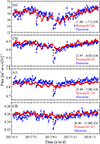 |
Fig. 1. Daily proton fluxes (red points) and electron fluxes (blue points) observed by AMS from May 5, 2017 to January 27, 2018 (a–d). The proton fluxes are divided by 67.60, 69.93, 91.18, and 107.47 within four rigidity bins for better comparison with electron fluxes. Data have not been published for protons at [1.00–1.71] GV from September 10, 2017 to September 15, 2017, and for electrons at [1.00–1.71] GV, [2.97–4.02] GV, [5.90–7.09] GV, and [8.48–11.00] GV on September 11, 2017 and September 12, 2017. |
 (1)
(1)
2.2. Hysteresis loop structure
The moving average of proton fluxes and electron fluxes for 2 BRs with a step of one day exhibits a loop structure from June 1, 2017 to December 31, 2017, as illustrated in Fig. 2.
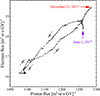 |
Fig. 2. Relationship between proton fluxes and electron fluxes at [1.00–1.71] GV, which are calculated by a moving average of 2BRs’ daily proton fluxes and electron fluxes with a step of one day as Aguilar et al. (2023). The violet and red arrows indicate the beginning and the end of the decline phase, while the gray arrows point in the direction of time increase. |
3. Method and model
Our simulation is based on the PTE. The method and model in our study are explained in detail in this section.
3.1. GCRs transport in the heliosphere and SDE approach
The propagation of GCRs in the heliosphere can be described by PTE (Potgieter 1998, 2013):
 (2)
(2)
where f(r, p, t) is the GCRs distribution function in phase space; r(r, θ, ϕ) is the spatial position of particles in spherical coordinate system; p represents particle momentum; VSW, ⟨VD⟩, and K(s) represent the solar wind velocity, the average of particle drift velocity, and the diffusion tensor, respectively. Equation (2) displays four physical mechanisms experienced by GCRs propagating in the heliosphere, that is, convection caused by the solar wind, drift caused by the curvature and gradient of IMF, diffusion resulting from magnetic turbulence in space, and adiabatic energy change due to the expansion of the solar wind. The cosmic ray flux, J, observed by space experiments can be represented by J = p2f (see more details in Potgieter 2013; Moraal 2013).
The PTE is solved by a set of time-backward SDEs,
 (3)
(3)
which is equivalent to PTE (Zhang 1999). Here, X is the particle location; s is the backward time; ασ is related to K(s) by  , with more details given in Zhang (1999); dWσ(s) is differential Wiener process and is given by the calculation of random numbers with standard normal distribution. The particle momentum, p, can be converted to rigidity P through P = pc/q, which is widely used in observation experiments. Here, c is the speed of light and q is the charge of the particle. Particles with initial momentum, p0, at an initial location (r0,θ0,ϕ0) move step by step, according to the SDEs until they arrived the heliopause (HP, the modulation boundary, is set as 122 AU in our simulation), where the momentum is taken as pb. The distribution function of particles with p0 at (r0,θ0,ϕ0) is
  , whereby fb(pb) is the distribution function of particles with momentum pb at the HP; N is the number of stochastic processes. Also, fb(pb) is obtained through the relationship
  , where Jb(Eb) is the flux of particles at the HP with energy Eb, calculated from the local interstellar spectrum (LIS); Jb(Pb) is the flux of particles at the HP with rigidity Pb; dP/dE is calculated based on
  ,
,  , where E is kinetic energy of protons (electrons) and E0 is the rest energy of protons (electrons), β is the particle velocity divided by speed of light, and dP/dE = 1/βb at the HP; then, βb = vb/c; vb is the velocity of particles with rigidity Pb; and, finally, c is the speed of light. The LISs in our simulation take the form described in Corti et al. (2016) for protons and in Potgieter et al. (2015) for electrons.
Main parameters of four DBs.
The solar wind velocity, VSW, displays an apparent latitude dependence around solar minimum (McComas et al. 2008), many researchers use solar wind models that vary along radial and latitude directions (Potgieter 2013; Potgieter et al. 2014, 2015; Song et al. 2021). We used a simplified latitude dependent model, defined within the termination shock (TS) as
 (4)
(4)
The radial outward solar wind speed is set as  between the TS and HP to satisfy ∇ ⋅ VSW = 0, which means the solar wind plasma between the TS and the HP is incompressible (Boschini et al. 2019). The location of the TS, rts, is set as 92 AU in our simulation. It should be noted that some research assumes that ∇ ⋅ VSW ≠ 0, for example, Langner et al. (2006), Baliukin et al. (2023).
We used Parker’s spiral magnetic field in our model, which can be described in spherical coordinates as
![Mathematical equation: $$ \begin{aligned} \boldsymbol{B}=\frac{AB_{0} }{r^{2} } \left( \hat{e_{r}} -\frac{r\Omega \sin \theta }{{V}_{\rm SW}} \hat{e_{\phi }} \right)\left[ 1-2H\left( \theta -\theta _{\rm cs} \right) \right], \end{aligned} $$](/articles/aa/full_html/2025/02/aa52416-24/aa52416-24-eq11.gif) (5)
(5)
where A = ±1 describe positive and negative solar polarity, respectively; r is the radial distance away from the Sun; θ is the polar angle; B0 is determined by the magnetic field at Earth’s location, Beq, with  ; Beq is set according to 13 months (14 BRs) running average of observations3, that is, the average of observations for previous 13 months, Beq and B0 are in units of nT, Ω is the solar rotation angular speed, while the solar rotation period is set as 27.27 days; H(θ−θcs) is the Heaviside function, expressed as
  ; θcs is the polar angle of the heliosphere current sheet (HCS), which is set according to 16 months (18 BRs) running average of observations4, as shown in Fig. 3. The time it takes for IMF and HCS to travel from the Sun to the HP is the basis for calculating the running average in our scenario. The weight of the volume of the slow and fast solar wind regions is utilized to calculate the IMF propagation speed. That is,
  km/s. The propagation speed of HCS is set as 430 km/s since the HCS tilt angle is in the slow solar wind region in the second half of 2017. Similar settings of the running average for B and HCS tilt angle can be found in Vos & Potgieter (2015). There are also some studies using different spread time, such as Tomassetti et al. (2017) and Bobik et al. (2012).
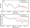 |
Fig. 3. Observations and running averages of the IMF magnitude and HCS tilt angle at Earth. Panel (a): observed 27 days average magnetic field magnitude at Earth between April 2016 and January 2018 (black squares and curve) and 13 months (14 BRs) running average (red points and curve). Panel (b): observed 27 days average HCS tilt angle at Earth between January 2016 and January 2018 (black squares and curve) and 16 months (18 BRs) running average (red points and curve). |
Particles also transport in the heliosphere with drift velocity  , where the drift coefficient
  . β is the ratio of particle velocity to the speed of light. According to previous studies, (κA)0 changes over time (Aslam et al. 2023a) and should be identical for protons and electrons (Aslam et al. 2023a; Potgieter et al. 2014, 2015). It is reasonable to assume (κA)0 is a constant during the cosmic ray declining phase because it is a short period compared to the solar cycle. The value of (κA)0 is taken as 0.9 for both protons and electrons in our simulation according to Aslam et al. (2023a).
The HCS is a structure where on both sides the direction of the magnetic field is reversed. Particles will drift along the HCS when their distance to the HCS surface, d, is close enough. We use d < 2Rg as criterion of the HCS drift in this study, where Rg is the particle gyro-radius in the IMF. The distance between particles at location (r,θ,ϕ) and HCS surface can be estimated by d = |r(θ−θcs)cotζ|, under the assumption of flat HCS, where ζ is the angle between the normal direction of the HCS, n, and the direction  . The magnitude of the HCS drift velocity,
  , is set, with
  correspondingly. Here, ψ stands for the IMF spiral angle. More details on the HCS drift velocity are given in Strauss et al. (2012), Luo et al. (2017).
The diffusion tensor K(s) can be shown as
 (6)
(6)
with the parallel and perpendicular diffusion coefficients, κ∥, ⊥, in our model take the following empirical form (Potgieter 2013),
 (7)
(7)
where the parameters a = 1, P0 = 1 GV are set during our simulation.
3.2. Diffusion barrier model
As the gyro-radius decreases in regions with an enhanced magnetic field, particles will be trapped in those areas. Regions with an enhanced magnetic field can be described as diffusion barriers, where diffusion and drift coefficients are assumed to be inversely proportional to the magnetic field strength. This means those coefficients will decrease in regions with enhanced magnetic field, effectively creating a barrier to the transport of GCRs. The concept of a diffusion barrier has been used in previous research. Perko & Fisk (1983) employed enhanced scattering regions, where the diffusion coefficient decreases, to describe the disturbance superposed on the undisturbed solar wind and to model the solar cycle variation in cosmic rays intensity; however, this model did not consider any drift effects. Such regions were identified as MIRs by Burlaga et al. (1985). They were regarded as turbulent boundary layers acting as barriers, blocking the propagation of cosmic rays toward the Sun. The GMIRs were simulated as large-scale regions spreading outward with lower diffusion and drift coefficients compared with background values (Haasbroek et al. 1995; Le Roux & Potgieter 1995; Luo et al. 2019). For a review, we refer to Potgieter (1998). Additionally, the concept of a propagating diffusion barrier is also used to simulate Forbush decreases lasting for several days, caused by the turbulent region (Luo et al. 2017, 2018).
We use a diffusion barrier (DB) model to describe the influence of solar wind structures with increased turbulent magnetic field on cosmic ray flux. Our DB model is a shell-like structure with thickness, L, which is divided to a leading part with width, ra, and a trailing part with width, rb, extending to θbr relative to the equatorial plane of the Sun and ϕbr around the Sun (see more details in Luo et al. 2011, 2019). The propagation velocities of DB inside and outside the TS are vu and vd, respectively, while the compression ratio of DB are cru and crd. The magnitude of the magnetic field at spatial location (r,θ,ϕ) increases from B to B′ when it encounters DB. As a result, diffusion and drift coefficients decrease in DB. We adopted the following formation (Luo et al. 2017):
 (8)
(8)
where κ∥, ⊥, A represent diffusion coefficients parallel and perpendicular to IMF and drift coefficient;  are the values in DB, ρ is a constant, f(r), h(θ), g(ϕ) describe the variation of coefficients along the radial distance from the Sun, latitude, and longitude, as shown in Eq. (9),
 (9)
(9)
where rsh(end) is the distance between the front (end) side of DB and the Sun, rcen = rsh − ra = rend + rb (Luo et al. 2017, 2019). The magnetic field increase factor is 1 + ρf(r)h(θ)g(ϕ). Both diffusion and drift coefficients reduce in DB, so as to simulate GCRs propagating barrier. If the barrier is 360° around the Sun, the longitude variation of the magnetic increase factor is ignored, which means g(ϕ) = 1 in our model. Detailed information on the DB parameters is shown in Sect. 4.
4. Results and discussion
Our strategy for studying the unusual flux changes is to begin with the simulation of the trend with DB model and then adjust the parameters used in the diffusion coefficients in the presence of DBs to ensure that the simulated flux results are in good agreement with the observed ones. Firstly, it is necessary to set reasonable DB parameters. We set two DBs according to the observation of interplanetary coronal mass ejections (CMEs) and another two DBs are set as GMIRs. We used daily [1.00–1.16] GV proton fluxes observed by AMS as the criterion for the adjustment of DBs parameters. Afterward, the parameters used in the expressions for diffusion coefficients were tuned day by day manually to simulate AMS observation data in four rigidity bins (as shown in Fig. 1). The hysteresis loop structure was plotted and explained subsequently. The proton spectra and electron spectra on several dates were calculated utilizing tuned parameters in the expressions for diffusion coefficients. We also analyzed the time dependence of parameters in the diffusion coefficients during this period, the time variation of the MFPs, and the rigidity dependence of MFPs on several dates.
4.1. Parameters of DBs and their effects on cosmic ray flux
Comparing the AMS published flux data with the observation of interplanetary CMEs5, we found that the two transient decreases in cosmic proton fluxes and electron fluxes coincided with the observed CMEs. Consequently, we set two separate DBs, DB1 and DB2, to simulate two CMEs. Parameters of two DBs are shown in Table 1. The propagation speed of two DBs are set as the average speed of CMEs by observation, while the thickness of two DBs are set according to the propagation speed multiple time that they passed the detector. And DB2 is mixed by events September 6, 2017 and September 7, 2017 through the convection of mass and momentum between them. The compression ratio and propagation speed of two DBs beyond the TS are fixed to 1.5 and 400 km/s, respectively. And we conjecture that there are two GMIRs, DB3 and DB4, in our model (rather than one) because the influence of one GMIR with two CMEs on cosmic ray flux is not consistent with AMS observation, shown in Fig. 4. The propagation speed of a GMIR up to the TS is ∼500 km/s (Whang et al. 1999; Luo et al. 2011, 2019). The DB1 and DB2 are set as Table 1, while DB3 is set as a GMIR with ra = 1 AU, rb = 9 AU, θbr = 60°, ϕbr = 360°, cru = 5, crd = 1.5, vu = 508 km/s, and vd = 400 km/s. The parameters of DB4 are the same as those of DB3. The speed of the four DBs remains constant during the process of moving away from the Sun. The subscripts u and d represent the areas inside and outside the termination shock, respectively. Actually, the cosmic proton fluxes need more time to recover as observed by AMS. Some details of the DBs we used in the reproduction of AMS observed proton fluxes and electron fluxes are shown in Table 1.
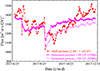 |
Fig. 4. Simulation results of 1.08 GV proton fluxes with DB1, DB2 and DB3 (magenta points), as well as with DB1, DB2, DB3, and DB4 (magenta circles), with comparison of [1.00–1.16] GV proton fluxes observed by AMS (red squares). |
Here, crd is fixed to 1.5, while vd is fixed to 400 km/s for four DBs. Figure 5 shows an example of the impact of four DBs on the IMF increase factor. Using these four DBs, we obtained the simulation results and deviations from the observations for proton fluxes at [1.00–1.16] GV from June 1, 2017 to December 31, 2017 (shown in Fig. 6). The parameters used in the expressions for the diffusion coefficients were set as κ0 = 311 × 1020cm2/s, b = 0.69, c = 3, d = 1.81, and Pk = 8.38 GV. The values of parameters b, c, d, and Pk were set according to the most probable value from Song et al. (2021). The AMS observation error, errAMSobs, and simulation deviation with observation devsim are defined by
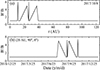 |
Fig. 5. Effects of four DBs shown as Table 1 on the magnitude of the IMF. Panel (a): radial variation of the increase factor in the equatorial plane (90°, 0°) on October 8, 2017. Panel (b): daily changes of increase factor at location (20 AU, 90° ,0° ). |
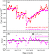 |
Fig. 6. Simulated proton fluxes using DBs shown in Fig. 5 and invariant parameters in the expressions of diffusion coefficients, as well as AMS observations of protons and the deviation of the two. Panel (a): [1.00–1.16] GV proton fluxes from AMS observation (red squares) with error bar and simulated 1.08 GV proton fluxes (magenta points) from June 1, 2017 to December 31, 2017. Panel (b): AMS observation error (gray shadow area) for [1.00–1.16] GV proton fluxes and simulation deviation (magenta points) for 1.08 GV proton fluxes from June 1, 2017 to December 31, 2017. |
 (10)
(10)
where JAMSerr, JAMSobs, Jsim represent the AMS observation flux error composed of the statistical and time-dependent systematic errors (Aguilar et al. 2021), AMS observation flux, and simulated flux, respectively. It is reasonable for us to draw the conclusion that the changes in fluxes during this period could be caused by CMEs and GMIRs (with the parameters listed in Table 1) because the simulation results can reproduce the proton flux trend well.
4.2. Simulation results with fine-tuning diffusion coefficients
We use proton fluxes and electron fluxes observed by AMS as reference to adjust parameters used in the expressions for the diffusion coefficients, until
 (11)
(11)
To reproduce the loop structure between the moving average of proton fluxes and electron fluxes, we simulated forward and backward for an additional 27 days, compared to the date range shown in Fig. 6. Proton fluxes and electron fluxes are simulated in four rigidity bins, namely: [1.00–1.71] GV, [2.97–4.02] GV, [5.90–7.09] GV, and [8.48–11.00] GV.
The AMS experiment has published daily proton fluxes in twelve smaller intervals for four rigidity bins, providing the possibility for more accurate simulation. Proton fluxes in twelve smaller rigidity bins can be aptly reproduced with our model during this period by adjusting the parameters, κ0, b, d, in diffusion coefficients day by day. The simulated daily proton fluxes at four rigidities and daily proton fluxes observed by AMS in four rigidity bins are shown in Fig. 7. Using the same method, simulated daily electron fluxes at four rigidities and daily electron fluxes in four rigidity bins observed by AMS are shown in Fig. 8. The values of the parameters κ0, b, d are detailed in Fig. 11. We obtained simulated proton fluxes at [1.00–1.71] GV from September 10, 2017 to September 15, 2017, and we simulated electron fluxes in four rigidity bins on September 11, 2017 and September 12, 2017, when AMS had not published their observation data. The simulation deviation significantly decreased, compared to when the parameters used in the expressions for the diffusion coefficients were kept constant, as shown in Fig. 6. The simulated proton fluxes at [1.00–1.71] GV are calculated according to Eq. (1), where fluxes at [1.00–1.16] GV, [1.16–1.33] GV, [1.33–1.51] GV, and [1.51–1.71] GV are represented by the simulation results at 1.08 GV, 1.24 GV, 1.42 GV, and 1.61 GV. The simulated electron fluxes at [1.00–1.71] GV were replaced by the simulated electron fluxes at 1.35 GV. We found the loop structure can be aptly reproduced by simulation results, as shown in Fig. 9.
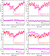 |
Fig. 7. Comparison between simulated proton fluxes at 1.08 GV, 3.13 GV, 6.18 GV, 10.55 GV (magenta points) and AMS observed proton fluxes at [1.00–1.16] GV, [2.97–3.29] GV, [5.90–6.47] GV, [10.10–11.00] GV (red squares) with error bars and corresponding AMS observation error (gray shadow areas) and simulation deviation (magenta points) from May 5, 2017 to January 27, 2018. |
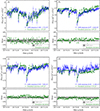 |
Fig. 8. Comparison between simulated electron fluxes at 1.35 GV, 3.49 GV, 6.49 GV, 9.74 GV (dark green points) and AMS observed electron fluxes at [1.00–1.71] GV, [2.97–4.02] GV, [5.90–7.09] GV, and [8.48–11.00] GV (blue squares) with error bars and corresponding AMS observation error (gray shadow areas), along with the simulation deviation (dark green points) from May 5, 2017 to January 27, 2018. |
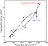 |
Fig. 9. Loop structure reproduced by simulated fluxes at [1.00–1.71] GV. Proton fluxes and electron fluxes are calculated with the moving average of 2BRs’ daily proton fluxes and electron fluxes with a step of one day. The violet arrow and red arrow indicate the beginning and the end of the decrease phase. The gray arrows point in the direction of time increase. |
Protons and electrons drift in opposite directions in the IMF due to their opposite charge. They will have the same drift speed when their rigidity is the same, while their diffusion coefficients are different during the decline phase (the difference is shown in Sect. 4.3). The formation of the electron–proton hysteresis loop structure is not only related to the drift mechanism, but also to diffusion. In this context, see also Aslam et al. (2023b).
We have been able to obtain daily spectra for protons and electrons at (1 AU, 90°, 0°). Figure 10 shows the comparison between AMS observations and simulated fluxes on four dates. The four dates contain the beginning of the study period (June 1, 2017), the end of the study period (December 31, 2017), the date with the minimum flux value after the first CME arrived at Earth (June 17, 2017), and the date with the minimum flux value after the second CME arrived at Earth (September 8, 2017). The spectra observed by AMS are well simulated using our method and model, with tuned parameters used in the expressions for diffusion coefficients (as shown in Fig. 11).
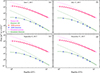 |
Fig. 10. Comparison between the simulated proton fluxes at (1 AU, 90°, 0°) (magenta lines) and proton fluxes observed by AMS (red triangles), as well as simulated electron fluxes at (1 AU, 90°, 0°) (dark green lines) and electron fluxes observed by AMS (blue triangles) on four dates, with respect to proton LIS (magenta dash lines) and electron LIS (dark green dash lines). |
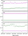 |
Fig. 11. Variation of parameters κ0, b, d in the diffusion coefficients (Eq. (7)) for protons (magenta points) and electrons (dark green points) from May 5, 2017 to January 27, 2018. The unit of κ0 is 1020 cm2 s−1. |
4.3. Variation of diffusion coefficients and MFPs
The daily alteration of parameters used in the expressions for the diffusion coefficients (Eq. (7)) is shown in Fig. 11. According to Song et al. (2021) and Potgieter et al. (2015), Pk = 8.38 GV, c = 3 for protons and Pk = 0.33 GV, b = 0, c = 3.5 for electrons are set as constants during our simulation. The three parameters show different time variations. For protons, the parameter κ0 exhibited significant changes, whereas parameters b and d only varied on several days with small changes. Parameters κ0 and d both show changes for electrons during this period. Using the relationship between MFPs, λ, and the diffusion coefficients, λ = 3κ/v, where v is the particle speed, daily proton MFPs and electron MFPs are available. Figure 12 shows the time variations of daily MFPs for protons and electrons at 1.08 GV (the rigidities used to simulate the proton fluxes at [1.00–1.16] GV observed by AMS) at (1 AU, 90°, 0°). It is revealed that different time variations of MFPs for protons and electrons are required for this period. Proton MFPs show two protuberances, which is related to GMIRs, while the electron MFPs increase when GMIRs are formed and then remain relatively stable. Rigidity dependence of parallel and perpendicular MFPs for protons and electrons at (1 AU, 90°, 0°) are plotted every ten days in Fig. 13 as an example. Parameters used in the expressions for the diffusion coefficients on some dates are the same, with details shown in Table 2. It is known that the effect of solar modulation on GCRs diminishes as their energy increases. Correspondingly, the MFPs for higher energy GCR should not vary with solar activity. The MFPs displayed in Fig. 13 do not illustrate clear convergence at high energy levels. In this sense, current form of MFPs for GCRs with higher energy need to be improved and used in the propagation of GCRs in the future.
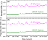 |
Fig. 12. Time variations of parallel (a) and perpendicular (b) MFPs for 1.08 GV protons (magenta points) and 1.08 GV electrons (dark green points) at (1 AU, 90°,0°) from May 5, 2017 to January 27, 2018. |
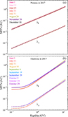 |
Fig. 13. Rigidity dependence of parallel (λ∥) and perpendicular (λ⊥) MFPs of protons (a) and electrons (b) at (1 AU, 90°,0°) for every 10 days from June 1, 2017 to December 31, 2017. Proton MFPs on August 20, 2017 are very close to the December 18, 2017 ones. For identification, we use dash black line to represent proton MFPs on December 18, 2017. Some of them are not shown because they are the same as other days (more details are displayed in Table 2). |
Date with the same value of parameters used in the expressions for the diffusion coefficients for every ten days.
The time variation of MFPs for protons at [1.00–1.16] GV and the rigidity dependence of MFPs for the period July 2006–November 2019 have been studied by Aslam et al. (2023b) using Carrington Rotation averaged spectra measured by PAMELA and AMS. The parallel MFP of protons at [1.00–1.16] GV in the second half of 2017 changed between approximately 0.8 AU and approximately 0.94 AU, while protons with rigidities ranging from 1.00 GV to 10.00 GV in June 2017 had the parallel MFP increasing from approximately 0.9 AU to approximately 20 AU in their study. However, the parallel MFP of protons at 1.08 GV varied between approximately 0.14 AU and approximately 0.19 AU, while protons with rigidities ranging from 1.00 GV to 10.00 GV mainly in the range of [0.1, 2] AU in our study. Our result is roughly five times smaller than the result reported by Aslam et al. (2023b). The parameters used in the expressions for diffusion coefficients (Eq. (7)) play an important role in the calculation of MFPs. The reason why our MFPs differ from theirs may be related to the availability of a suitable parameter space to appropriately simulate the observations.
5. Summary and conclusions
The AMS experiment has published daily proton fluxes and electron fluxes from May 2011 to November 2021. In the second half of 2017, both proton fluxes and electron fluxes exhibited large decreases and the electron–proton hysteresis was different from other periods; that is, a loop structure appeared. Aiming to find the reason for the unusual changes in proton fluxes and electron fluxes observed by AMS in the second half of 2017 and clarifying the solar modulation mechanism for the formation of the loop structure, a 3D numerical model based on Parker transport equation combing with the propagating DB model was used to simulate the AMS daily proton fluxes and electron fluxes. In this model, four modulation mechanisms, namely, convection, drift, diffusion, and adiabatic energy change, are included. The solar wind speed was set as simplified latitude dependent form as Eq. (4). The time-varying HCS tilt angle and IMF magnitude were used to reflect the solar activity. The diffusion coefficients have the same expression for protons and electrons (Eq. (7), for electrons, b = 0). In addition, the drift coefficient (κA)0 = 0.9 was used for both protons and electrons. We used the DB model, in which diffusion and drift coefficients will decrease, to simulate the effects of CMEs and GMIRs. The LISs utilized in our simulation are from Corti et al. (2016) and Potgieter et al. (2015). The parameters used in the expressions of diffusion coefficients (Eq. (7)), κ0, b, and d, were adjusted day by day to reproduce the daily proton fluxes and electron fluxes observed by AMS.
Although there should be an adequate parameter space for κ0, b, and d to reproduce the AMS observed cosmic ray fluxes well, because κ0, b, d are mutually dependent, we obtained one set of parameters and we have drawn our conclusions on this basis. We find that:
-
The CMEs and GMIRs could be the main driver for the unusual changes of proton fluxes and electron fluxes seen in the second half of 2017. We used the DB model to simulate the influence of CMEs and GMIRs. The parameters of two DBs used to simulate CMEs were set according to the interplanetary CME observation, while the parameters of the other two DBs designed to simulate GMIRs were set based on the previous studies and tuned by daily proton fluxes at [1.00–1.16] GV observed by AMS, as shown in Table 1. The simulated proton flux trend, with unchanged parameters used in the expressions for the diffusion coefficients, closely resembles the AMS observed trend as depicted in Fig. 6.
-
When considering CMEs and GMIRs, proton fluxes and electron fluxes as well as the electron–proton hysteresis loop structure during this period can be well reproduced by tuning three parameters used in the expression of diffusion coefficients. This also indicates that the appearance of the loop structure is related not only to drift mechanism, but to diffusion as well. Three parameters used in the expression for diffusion coefficients for protons and electrons, κ0, b, and d, demonstrate different time variations (as shown in Fig. 11). Using these three tuned parameters, the proton spectrum and electron spectrum observed by AMS are well simulated (such as shown in Fig. 10).
-
The daily MFPs of protons and electrons have different time variations and rigidity dependence during the second half of 2017. When GMIRs arise, MFPs increase for both protons and electrons at (1 AU, 90°, 0°). Proton MFPs then exhibit two protuberances, whereas electron MFPs stay comparatively stable as shown in Fig. 12. The rigidity dependence of MFPs for protons and electrons is different, and the rigidity dependence of protons (electrons) also varies on different dates, as shown in Fig. 13.
The current study is based on the daily fluxes of protons and electrons. As the AMS experiment provides more accurate flux measurements of various cosmic ray compositions, with our unique numerial model more insights about cosmic ray solar modualtion can be gained. Specifically, our understanding for the charge-sign and charge-mass ratio effects can be further improved.
Data from https://www.nmdb.eu/
Data from https://lpsc.in2p3.fr/crdb/
Data from https://omniweb.gsfc.nasa.gov
Data from http://wso.stanford.edu.
Acknowledgments
The data for this work are provided by the NMDB database (www.nmdb.eu), founded under the European Union’s FP7 program (contract no. 213007) and Near-Earth Interplanetary Coronal Mass Ejections Since January 1996 (https://doi.org/10.7910/DVN/C2MHTH). The present work is jointly supported by the startup funding of the Shandong Institute of Advanced Technology No. 2020106R01, Taishan Scholar Project of Shandong Province No. 202103143, and NSFC grants No. U2106201.
References
- Aguilar, M., Cavasonza, L. A., Ambrosi, G., et al. 2021, Phys. Rev. Lett., 127, 271102 [NASA ADS] [CrossRef] [Google Scholar]
- Aguilar, M., Cavasonza, L. A., Ambrosi, G., et al. 2023, Phys. Rev. Lett., 130, 161001 [Google Scholar]
- Aslam, O. P. M., Luo, X., Potgieter, M. S., Ngobeni, M. D., & Song, X. 2023a, ApJ, 947, 72 [NASA ADS] [CrossRef] [Google Scholar]
- Aslam, O. P. M., Potgieter, M. S., Luo, X., & Ngobeni, M. D. 2023b, ApJ, 953, 101 [NASA ADS] [CrossRef] [Google Scholar]
- Baliukin, I. I., Izmodenov, V. V., & Alexashov, D. B. 2023, MNRAS, 525, 3281 [NASA ADS] [CrossRef] [Google Scholar]
- Belov, A. 2000, Space Sci. Rev., 93, 79 [NASA ADS] [CrossRef] [Google Scholar]
- Bindi, V., Corti, C., Consolandi, C., Hoffman, J., & Whitman, K. 2017, Adv. Space Res., 60, 865 [NASA ADS] [CrossRef] [Google Scholar]
- Bobik, P., Boella, G., Boschini, M. J., et al. 2012, ApJ, 745, 132 [Google Scholar]
- Boschini, M. J., Della Torre, S., Gervasi, M., La Vacca, G., & Rancoita, P. G. 2019, Adv. Space Res., 64, 2459 [NASA ADS] [CrossRef] [Google Scholar]
- Burlaga, L. F., McDonald, F. B., Goldstein, M. L., & Lazarus, A. J. 1985, J. Geophys. Res. Space Phys., 90, 12027 [NASA ADS] [CrossRef] [Google Scholar]
- Burlaga, L. F., McDonald, F. B., & Ness, N. F. 1993, J. Geophys. Res. Space Phys., 98, 1 [NASA ADS] [CrossRef] [Google Scholar]
- Corti, C., Bindi, V., Consolandi, C., & Whitman, K. 2016, ApJ, 829, 8 [Google Scholar]
- Engelbrecht, N. E., Effenberger, F., Florinski, V., et al. 2022, Space Sci. Rev., 218, 33 [CrossRef] [Google Scholar]
- Haasbroek, L. J., Potgieter, M. S., & Le Roux, J. A. 1995, Adv. Space Res., 16, 209 [NASA ADS] [CrossRef] [Google Scholar]
- Langner, U. W., Potgieter, M. S., Fichtner, H., & Borrmann, T. 2006, ApJ, 640, 1119 [NASA ADS] [CrossRef] [Google Scholar]
- Le Roux, J. A., & Potgieter, M. S. 1995, ApJ, 442, 847 [NASA ADS] [CrossRef] [Google Scholar]
- Luo, X., Zhang, M., Rassoul, H. K., & Pogorelov, N. V. 2011, ApJ, 730, 13 [Google Scholar]
- Luo, X., Potgieter, M. S., Zhang, M., & Feng, X. 2017, ApJ, 839, 53 [NASA ADS] [CrossRef] [Google Scholar]
- Luo, X., Potgieter, M. S., Zhang, M., & Feng, X. 2018, ApJ, 860, 160 [NASA ADS] [CrossRef] [Google Scholar]
- Luo, X., Potgieter, M. S., Bindi, V., Zhang, M., & Feng, X. 2019, ApJ, 878, 6 [NASA ADS] [CrossRef] [Google Scholar]
- McComas, D. J., Ebert, R. W., Elliott, H. A., et al. 2008, Geophys. Res. Lett., 35, L18103 [NASA ADS] [CrossRef] [Google Scholar]
- McDonald, F. B. 1998, Space Sci. Rev., 83, 33 [NASA ADS] [CrossRef] [Google Scholar]
- Moraal, H. 2013, Space Sci. Rev., 176, 299 [CrossRef] [Google Scholar]
- Parker, E. N. 1965, Planet Space Sci., 13, 9 [CrossRef] [Google Scholar]
- Perko, J., & Fisk, L. 1983, J. Geophys. Res. Space Phys, 88, 9033 [NASA ADS] [CrossRef] [Google Scholar]
- Potgieter, M. S. 1998, Space Sci. Rev., 83, 147 [CrossRef] [Google Scholar]
- Potgieter, M. S. 2013, Living Rev. Sol. Phys., 10, 1 [NASA ADS] [CrossRef] [Google Scholar]
- Potgieter, M. S., & Le Roux, J. A. 1994, ApJ, 423, 817 [NASA ADS] [CrossRef] [Google Scholar]
- Potgieter, M. S., Vos, E. E., Boezio, M., et al. 2014, Sol. Phys., 289, 391 [NASA ADS] [CrossRef] [Google Scholar]
- Potgieter, M. S., Vos, E. E., Munini, R., Boezio, M., & Di Felice, V. 2015, ApJ, 810, 141 [NASA ADS] [CrossRef] [Google Scholar]
- Rankin, J. S., Bindi, V., Bykov, A. M., et al. 2022, Space Sci. Rev., 218, 42 [NASA ADS] [CrossRef] [Google Scholar]
- Song, X., Luo, X., Potgieter, M. S., Liu, X., & Geng, Z. 2021, ApJS, 257, 48 [NASA ADS] [CrossRef] [Google Scholar]
- Strauss, R. D., Potgieter, M. S., Buesching, I., & Kopp, A. 2012, Ap&SS, 339, 223 [NASA ADS] [CrossRef] [Google Scholar]
- Tomassetti, N., Orcinha, M., Barao, F., & Bertucci, B. 2017, ApJ, 849, L32 [NASA ADS] [CrossRef] [Google Scholar]
- Vos, E. E., & Potgieter, M. S. 2015, ApJ, 815, 119 [NASA ADS] [CrossRef] [Google Scholar]
- Whang, Y. C., Lu, J. Y., & Burlaga, L. F. 1999, J. Geophys. Res. Space Phys, 104, 19787 [NASA ADS] [CrossRef] [Google Scholar]
- Zhang, M. 1999, ApJ, 513, 409 [NASA ADS] [CrossRef] [Google Scholar]
All Tables
Date with the same value of parameters used in the expressions for the diffusion coefficients for every ten days.
All Figures
|
Fig. 1. Daily proton fluxes (red points) and electron fluxes (blue points) observed by AMS from May 5, 2017 to January 27, 2018 (a–d). The proton fluxes are divided by 67.60, 69.93, 91.18, and 107.47 within four rigidity bins for better comparison with electron fluxes. Data have not been published for protons at [1.00–1.71] GV from September 10, 2017 to September 15, 2017, and for electrons at [1.00–1.71] GV, [2.97–4.02] GV, [5.90–7.09] GV, and [8.48–11.00] GV on September 11, 2017 and September 12, 2017. |
| In the text | |
|
Fig. 2. Relationship between proton fluxes and electron fluxes at [1.00–1.71] GV, which are calculated by a moving average of 2BRs’ daily proton fluxes and electron fluxes with a step of one day as Aguilar et al. (2023). The violet and red arrows indicate the beginning and the end of the decline phase, while the gray arrows point in the direction of time increase. |
| In the text | |
|
Fig. 3. Observations and running averages of the IMF magnitude and HCS tilt angle at Earth. Panel (a): observed 27 days average magnetic field magnitude at Earth between April 2016 and January 2018 (black squares and curve) and 13 months (14 BRs) running average (red points and curve). Panel (b): observed 27 days average HCS tilt angle at Earth between January 2016 and January 2018 (black squares and curve) and 16 months (18 BRs) running average (red points and curve). |
| In the text | |
|
Fig. 4. Simulation results of 1.08 GV proton fluxes with DB1, DB2 and DB3 (magenta points), as well as with DB1, DB2, DB3, and DB4 (magenta circles), with comparison of [1.00–1.16] GV proton fluxes observed by AMS (red squares). |
| In the text | |
|
Fig. 5. Effects of four DBs shown as Table 1 on the magnitude of the IMF. Panel (a): radial variation of the increase factor in the equatorial plane (90°, 0°) on October 8, 2017. Panel (b): daily changes of increase factor at location (20 AU, 90° ,0° ). |
| In the text | |
|
Fig. 6. Simulated proton fluxes using DBs shown in Fig. 5 and invariant parameters in the expressions of diffusion coefficients, as well as AMS observations of protons and the deviation of the two. Panel (a): [1.00–1.16] GV proton fluxes from AMS observation (red squares) with error bar and simulated 1.08 GV proton fluxes (magenta points) from June 1, 2017 to December 31, 2017. Panel (b): AMS observation error (gray shadow area) for [1.00–1.16] GV proton fluxes and simulation deviation (magenta points) for 1.08 GV proton fluxes from June 1, 2017 to December 31, 2017. |
| In the text | |
|
Fig. 7. Comparison between simulated proton fluxes at 1.08 GV, 3.13 GV, 6.18 GV, 10.55 GV (magenta points) and AMS observed proton fluxes at [1.00–1.16] GV, [2.97–3.29] GV, [5.90–6.47] GV, [10.10–11.00] GV (red squares) with error bars and corresponding AMS observation error (gray shadow areas) and simulation deviation (magenta points) from May 5, 2017 to January 27, 2018. |
| In the text | |
|
Fig. 8. Comparison between simulated electron fluxes at 1.35 GV, 3.49 GV, 6.49 GV, 9.74 GV (dark green points) and AMS observed electron fluxes at [1.00–1.71] GV, [2.97–4.02] GV, [5.90–7.09] GV, and [8.48–11.00] GV (blue squares) with error bars and corresponding AMS observation error (gray shadow areas), along with the simulation deviation (dark green points) from May 5, 2017 to January 27, 2018. |
| In the text | |
|
Fig. 9. Loop structure reproduced by simulated fluxes at [1.00–1.71] GV. Proton fluxes and electron fluxes are calculated with the moving average of 2BRs’ daily proton fluxes and electron fluxes with a step of one day. The violet arrow and red arrow indicate the beginning and the end of the decrease phase. The gray arrows point in the direction of time increase. |
| In the text | |
|
Fig. 10. Comparison between the simulated proton fluxes at (1 AU, 90°, 0°) (magenta lines) and proton fluxes observed by AMS (red triangles), as well as simulated electron fluxes at (1 AU, 90°, 0°) (dark green lines) and electron fluxes observed by AMS (blue triangles) on four dates, with respect to proton LIS (magenta dash lines) and electron LIS (dark green dash lines). |
| In the text | |
|
Fig. 11. Variation of parameters κ0, b, d in the diffusion coefficients (Eq. (7)) for protons (magenta points) and electrons (dark green points) from May 5, 2017 to January 27, 2018. The unit of κ0 is 1020 cm2 s−1. |
| In the text | |
|
Fig. 12. Time variations of parallel (a) and perpendicular (b) MFPs for 1.08 GV protons (magenta points) and 1.08 GV electrons (dark green points) at (1 AU, 90°,0°) from May 5, 2017 to January 27, 2018. |
| In the text | |
|
Fig. 13. Rigidity dependence of parallel (λ∥) and perpendicular (λ⊥) MFPs of protons (a) and electrons (b) at (1 AU, 90°,0°) for every 10 days from June 1, 2017 to December 31, 2017. Proton MFPs on August 20, 2017 are very close to the December 18, 2017 ones. For identification, we use dash black line to represent proton MFPs on December 18, 2017. Some of them are not shown because they are the same as other days (more details are displayed in Table 2). |
| In the text | |
Current usage metrics show cumulative count of Article Views (full-text article views including HTML views, PDF and ePub downloads, according to the available data) and Abstracts Views on Vision4Press platform.
Data correspond to usage on the plateform after 2015. The current usage metrics is available 48-96 hours after online publication and is updated daily on week days.
Initial download of the metrics may take a while.