| Issue |
A&A
Volume 690, October 2024
|
|
|---|---|---|
| Article Number | A66 | |
| Number of page(s) | 28 | |
| Section | Extragalactic astronomy | |
| DOI | https://doi.org/10.1051/0004-6361/202348141 | |
| Published online | 01 October 2024 | |
The host of GRB 171205A in 3D
A resolved multiwavelength study of a rare grand-design spiral GRB host
1
Astronomical Institute, Czech Academy of Sciences, Fričova 298, Ondřejov, Czech Republic
2
Université de la Côte d’Azur, Observatoire de la Côte d’Azur, CNRS, 06304 Nice, France
3
Aix Marseille Univ., CNRS, CNES, LAM, Marseille, France
4
INAF, Osservatorio Astronomico di Capodimonte, Salita Moiariello 16, 80131 Napoli, Italy
5
DARK, Niels Bohr Institute, University of Copenhagen, Jagtvej 128, 2200-N Copenhagen, Denmark
6
Astronomical Observatory Institute, Faculty of Physics, Adam Mickiewicz University, ul. Słoneczna 36, 60-286 Poznań, Poland
7
Department of Astrophysics/IMAPP, Radboud University, 6525 AJ Nijmegen, The Netherlands
8
David A. Dunlap Department of Astronomy & Astrophysics, University of Toronto, 50 St. George St., Toronto, Ontario M5S 3H4, Canada
9
Centro Astronómico Hispano-Alemán, Observatorio de Calar Alto, Sierra de los Filabres, 4550 Gérgal, Spain
10
3 Dunlap Institute for Astrophysics & Astrophysics, University of Toronto, 50 St. George Street, Toronto, ON M5S 3H4, Canada
11
Racah Institute of Physics, The Hebrew University of Jerusalem, Jerusalem 91904, Israel
12
Cosmic Dawn Center, Niels Bohr Institute, University of Copenhagen, Jagtvej 128, 2200-N Copenhagen, Denmark
13
INAF, Osservatorio Astronomico di Brera, Via Bianchi, Merate, Italy
14
Space Science Data Center (SSDC) – Agenzia Spaziale Italiana (ASI), 00133 Roma, Italy
15
INAF – Osservatorio Astronomico di Roma, Via Frascati 33, 00040 Monte Porzio Catone, Italy
16
Clemson University, Department of Physics and Astronomy, Clemson, SC 29634-0978, USA
17
Centre for Astrophysics and Cosmology, Science Institute, University of Iceland, Dunhagi 5, 107 Reykjavík, Iceland
18
University of Messina, MIFT Department, Via F. S. D’Alcontres 31, Papardo, 98166 Messina, Italy
19
Astronomical Institute Anton Pannekoek, University of Amsterdam, 1090 GE Amsterdam, The Netherlands
20
INAF – Osservatorio di Astrofisica e Scienza dello Spazio, Via Piero Gobetti 93/3, 40129 Bologna, Italy
21
Department of Physics, University of Bath, Bath BA2 7AY, UK
22
Centre for Astrophysics Research, University of Hertfordshire, Hatfield AL10 9AB, UK
23
School of Mathematical and Physical Sciences, Macquarie University, NSW 2109, Australia
24
ARC Centre of Excellence for All Sky Astrophysics in 3 Dimensions (ASTRO-3D), Australia
Received:
3
October
2023
Accepted:
2
July
2024
Abstract
Long GRB hosts at z < 1 are usually low-mass, low-metallicity star-forming galaxies. Here we present the most detailed, spatially resolved study of the host of GRB 171205A so far, a grand-design barred spiral galaxy at z = 0.036. Our analysis includes MUSE integral field spectroscopy complemented with high-spatial-resolution UV/VIS HST imaging and CO(1−0) and H I 21 cm data. The GRB is located in a small star-forming region in a spiral arm of the galaxy at a deprojected distance of ∼8 kpc from the center. The galaxy shows a smooth negative metallicity gradient and the metallicity at the GRB site is half solar, slightly below the mean metallicity at the corresponding distance from the center. Star formation in this galaxy is concentrated in a few H II regions between 5 and 7 kpc from the center and at the end of the bar, inwards from the GRB region; however the H II region hosting the GRB is in the top 10% of the regions with the highest specific star-formation rate. The stellar population at the GRB site has a very young component (< 5 Myr) that contributes a significant part of the light. Ionized and molecular gas show only minor deviations at the end of the bar. A parallel study found an asymmetric H I distribution and some additional gas near the position of the GRB, which might explain the star-forming region of the GRB site. Our study shows that long GRBs can occur in many types of star-forming galaxies; however the actual GRB sites have consistently low metallicity, high star formation rates, and a young population. Furthermore, gas inflow or interactions triggering the star formation producing the GRB progenitor might not be evident in ionized or even molecular gas but only in H I.
Key words: galaxies: ISM / galaxies: kinematics and dynamics / galaxies: spiral / gamma-ray burst: individual: GRB 171205A
Corresponding author; This email address is being protected from spambots. You need JavaScript enabled to view it. .
© The Authors 2024
 Open Access article, published by EDP Sciences, under the terms of the Creative Commons Attribution License (https://creativecommons.org/licenses/by/4.0), which permits unrestricted use, distribution, and reproduction in any medium, provided the original work is properly cited.
This article is published in open access under the Subscribe to Open model. This email address is being protected from spambots. You need JavaScript enabled to view it. to support open access publication.
1. Introduction
Long-duration gamma-ray bursts (GRBs) are the most luminous stellar explosions in the Universe. They originate from the collapse of a massive star –possibly a Wolf-Rayet star– stripped of its hydrogen and helium envelope while retaining a high angular momentum to support an accretion disk and launch a jet. In addition to synchrotron emission from the jet created in the actual GRB, the star explodes as a broad-line (BL) Ic supernova (SN) (Hjorth et al. 2003; Modjaz et al. 2016; Cano et al. 2017a). In recent years, a few exceptions have been found that might point to different progenitors or may alternatively be compact binary mergers accompanied by a kilonova instead of a BL-Ic SN (Fynbo et al. 2006; Michałowski et al. 2015; Rastinejad et al. 2022), which would be typical for a short GRB. The peak absolute magnitudes of GRB-SNe are in the range of MR = −18.5 to −20 mag (Cano et al. 2017a), making their detection at redshifts above ∼1 challenging. Furthermore, the average GRB redshift is z ∼ 2.2 and events at z < 0.5 –where we can obtain high-signal-to-noise-ratio (S/N) spectra and spectral series– are rare.
Studies of GRB hosts suffer from the same redshift problem as studies of GRB-SNe: spatially resolving them is only possible at low redshifts with current ground-based instrumentation and is still challenging at higher redshift in the NIR with JWST (Schady et al. 2024). Various studies of global host properties have shown that long GRB hosts are all actively star forming and have predominantly low metallicities (Krühler et al. 2015), although there are exceptions (Savaglio et al. 2012; Schady et al. 2015; Michalowski et al. 2018; Heintz et al. 2018). Long-GRB hosts at low redshifts furthermore have low average masses of < 1/10 L* (the luminosity of a Milky-Way galaxy), but tend to higher masses at redshifts beyond 2 (Perley et al. 2016; Palmerio et al. 2019). L* hosts at redshifts of z ≲ 1 are extremely rare, and most hosts are dwarf compact or irregular galaxies. The host of GRB 171205A is the first grand design spiral long GRB host at z < 0.5, and its discovery was only recently followed by that of the even larger spiral host galaxy of GRB 190829A (Dichiara et al. 2019).
Studying the global properties of a host galaxy might not necessarily reflect the conditions at the GRB site. Due to the low number of hosts at z < 0.4 –where all important emission lines are still in the visible part of the spectrum–, the faintness and small size of the hosts, and the lack of very sensitive integral field units (IFUs) needed, there are still only a few long GRB hosts that have been studied at high angular resolution: GRBs 980425 (Christensen et al. 2008; Krühler et al. 2017), 060505 (Thöne et al. 2014), 111005A (Tanga et al. 2018; Michalowski et al. 2018), and 100316D (Izzo et al. 2017), and only three short GRB hosts: GRBs 170817 (Levan et al. 2017), 050709 (Nicuesa Guelbenzu et al. 2021b), and 080905A (Nicuesa Guelbenzu et al. 2021a). A few other GRB hosts have been observed at low resolution with one or several long slit positions: GRB 120422A (Schulze et al. 2014), GRB 161219B (Cano et al. 2017b), and the short GRB 130603B (de Ugarte Postigo et al. 2014a). These studies indicate that long GRBs tend to occur in the more metal poor and more highly star-forming regions of their galaxies; although in most galaxies, the GRB site is not the site with the most extreme properties. However, all GRB sites consistently show a subsolar metallicity, which is believed to be necessary to produce a long GRB by theoretical models (Yoon et al. 2006); although binary progenitors might change the picture (Chrimes et al. 2020). GRB-SNe as well as BL-Ic SNe without GRBs also seem to have lower-metallicity progenitors than normal Ic SNe, pointing to a similar progenitor and possibly a choked jet for BL-Ics without GRBs (Modjaz et al. 2020). In a recent study of resolved kinematics in six GRB hosts (Thöne et al. 2021), all hosts show evidence of large-scale outflows or winds, confirming the highly star-forming nature of GRB hosts. Models have proposed that GRB progenitors are Wolf-Rayet (WR) stars (Woosley & Heger 2006; Detmers et al. 2008), that is, stripped stars originating from stars at > 20−30 M⊙ with a lifetime of only a few million years, which strengthens the connection to recent, massive star formation generally observed in long GRB hosts.
One of the few very nearby GRBs was GRB 171205A, which was detected by the Swift satellite on 5 Dec. 2017, with a duration in γ-rays of T90 = 189 s and at a distance of only 163 Mpc or z = 0.037 (Izzo et al. 2019). This was a low-luminosity GRB, which is the predominant class of long GRBs, but due to their faintness they can only be observed at low redshift (Liang et al. 2007; Patel et al. 2023). We initiated an early observing campaign and detected the first traces of the SN only one day after explosion (de Ugarte Postigo et al. 2017). We observed two different components in the SN: an early component with fast ejecta and an inverted composition, which was interpreted as emission from a cocoon around the emerging GRB jet (Izzo et al. 2019), and a later component with rather standard GRB-SN features. The proximity allowed us to observe this SN into the nebular phase, yielding one of the longest and highest-cadence follow-up datasets of a GRB-SN obtained so far (de Ugarte Postigo et al., in prep.). The host is a high-mass, grand-design spiral with log10(M/M⊙) 10.29 (de Ugarte Postigo et al. 2024), which is an unusual type for a long-GRB host galaxy (see e.g., Fruchter et al. 2006; Schneider et al. 2022).
In this paper, we present extensive multiwavelength data for the host galaxy of GRB 171205A, focusing in particular on the IFU dataset obtained with the Multi-Unit Spectroscopic Explorer (MUSE) at the Very Large Telescope (VLT), complemented with CO(1−0) observations with the Atacama Large Millimetre Array (ALMA), H I observations of the 21 cm line with the Giant Meterwave Radio Telescope (GMRT) (both datasets are presented in de Ugarte Postigo et al. 2024) and the Very Large Array (VLA), as well as imaging with the HST in UV and visible bands. In Sects. 2 and 3, we present the observations and our analysis of the MUSE datacube and the auxiliary data. In Sect. 4, we present the results from our spatially resolved study, and in Sect. 5 we show the resolved kinematics of the host using ionized, molecular, and neutral gas. Finally, in Sect. 6 we discuss our results and compare the host and the GRB site to other GRB hosts at low redshift. Throughout the paper we use a flat lambda CDM cosmology as constrained by Planck with Ωm = 0.315, ΩΛ = 0.685, and H0 = 67.3 km s−1 Mpc−1 (Planck Collaboration VI 2020).
2. Observations and data analysis
2.1. IFU data and additional spectroscopy
We observed the host galaxy of GRB 171205A (6dFGS gJ110939.7−123512, Jones et al. 2009) with the integral-field unit MUSE instrument mounted on the UT4 at the European Southern Observatory in Paranal (Chile). Observations started on March 20, 2018, i.e. 105 days after the GRB detection, and consisted of four exposure of 900 s each in wide field mode. These observations were obtained within the Stargate program1. The raw data were reduced using a set of ESOREX scripts (v. 3.13.7) that provide a fully combined and flux-calibrated datacube, which was used for the analysis presented in this paper. MUSE spaxels (in IFU data each “pixel” in the spatial direction also contains spectral information and is hence called a “spaxel”) have a size of  ; however, due to the seeing conditions, the actual resolution is
  , corresponding to a physical resolution of 0.5 kpc. The observing log of this and all other observations used in this paper is displayed in Table 1.
Log of the observations used in this paper. The last column refers to the presence or absence of the underlying GRB-SN.
Additional data of the environment of SN 2017iuk were obtained 14 months after the SN explosion with X-shooter at the VLT. A set of eight exposures of 300 s were obtained in the three arms of X-shooter on February 14, 2019, using the ABBA nod-on-slit method, with a nod throw of 6 arcsec along the slit. The data were not reduced using the X-shooter nodding mode pipeline, instead we reduced each single spectrum as if it had been obtained without any offset along the slit (stare mode). Given that the full 11 arcsec length of the X-shooter slit was entirely within the host galaxy, a conventional background subtraction was not possible. To correct the sky background in these spectra we used the Cerro Paranal Advanced Sky Model provided by ESO (Noll et al. 2012; Jones et al. 2013). In spite of the quality of this model it is never as precise as an observed correction and this could be the reason for the small wiggles seen in the resulting spectra (see Fig. 1). The spectral series have finally been stacked to result in a spectrum of the immediate environment of SN 2017iuk, but contaminated by sky emission lines and continuum.
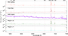 |
Fig. 1. Integrated spectra and detected lines in (top to bottom): the integrated galaxy spectrum, the galaxy core and bar, the GRB region, and H II regions 15 and 17, which show a very young stellar population. |
We also obtained IFU data of a companion galaxy at a distance of 186 kpc discovered originally in H I to have the same redshift and which could have interacted with the host (see Sect. 6). The data have been presented already in de Ugarte Postigo et al. (2024), but they only show the integrated spectrum and do not list emission line fluxes. The galaxy was observed with the Potsdam Multi-Aperture Spectrophotometer (PMAS) mounted on the 3.5 m telescope of Calar Alto Observatory (Spain; Roth et al. 2005) using the  lens array, which gives a field-of-view of 16″ × 16″2. We used the V500 grism, providing a wavelength coverage from 3700−7700 Å at an average spectral resolution of ∼4.3 Å at a rotation angle of 143.5 deg. Four pointings were needed to cover the galaxy. Data reduction was done with the P3D reduction tools (Sandin et al. 2010) and the different pointings combined to a single cube.
2.2. Imaging data from HST
We obtained observations of GRB 171205A and its host galaxy with the Hubble Space Telescope (HST). Observations were obtained at three epochs on 25 December 2017 using filter F300X, on 2 July 2018 in filters F300X, F475W and F606W, and a final epoch on 2 December 2019 using F300X, F475W and F606W (1083 s). The last images were taken two years after the GRB, and therefore we expected the contribution from the afterglow or supernova to be minimal.
The imaging data were retrieved from the HST archive after standard processing (debiasing, flat-fielding and charge transfer efficiency corrections). The data were subsequently drizzled via astrodrizzle to a plate scale of 0.025 arcsec per pixel. A color composite image of the second epoch images is shown in Fig. 2. The last epoch at two years post GRB reveals an H II region right at the location of the GRB, making an association of this region to the progenitor site of the event very likely.
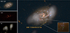 |
Fig. 2. Multi-color image of the host of GRB 171205A. Small panels, top left: False-color image based on HST images in filters F606W (red), F473W (green), and F300X (blue) taken in July 2018 with the GRB-SN still present. Center left: CO(1−0) emission from ALMA. Bottom left: H I emission from JVLA, including contours. Large panel: False-color image combining the HST data together with the CO(1−0) emission from ALMA (dark red) and H I emission from JVLA (white clouds). The inset shows data from December 2019 when the SN had faded and revealed the underlying star-forming region at the GRB site, marked by a green circle. In all images, north is up and east is left. |
2.3. Long-wavelength data
Our study is complemented with data from ALMA and GMRT already presented in de Ugarte Postigo et al. (2024) as well as data from the JVLA (Arabsalmani et al. 2022). ALMA Band 3 observations covering CO(1−0) at the redshift of the host were taken on Dec. 7 and 8, 2017 with a total integration time of 4.9 h. The data have a spectral resolution of 0.977 MHz or ∼2.6 km s−1 and a spatial resolution of  . Data were calibrated with Common Astronomy Software Applications (CASA) (McMullin et al. 2007; CASA Team 2022), smoothed to 10 km s−1, which yields an rms of 0.2 mJy and continuum subtracted. GMRT observed the field with a total time of 12 h distributed in two epochs at an observing frequency of 1.362 GHz, a total bandwidth of 16.7 MHz, and a channel width of 32.6 kHz, equivalent to 7 km s−1 (de Ugarte Postigo et al. 2024). The data were reduced with the in the Astronomical Image Processing software (van Moorsel et al. 1996) and combined to a single cube. The final cubes have beam sizes of 13″ × 19″ and 21″ × 27″.
We redid the analysis of the data taken by JVLA, which observed the field for 10.5 h over two epochs on 9 Mar. 2019 and 4 May 2019 (proposal ID: VLA/19A-394; Arabsalmani et al. 2022). The observing frequency of 1.368 GHz, with a channel width of 3.9 kHz and a 16 MHz bandwidth, which is equivalent to a velocity resolution of 0.8 km s−1 and a total velocity coverage of 3500 km s−1, and have a beam size of  .
.
The standard pipeline-calibrated data (Kent et al. 2020)3 were processed through standard procedures in CASA. Corrupted visibility was flagged before the datasets from the two epochs were combined together. On the combined dataset, we used the line-free data to produce a standard continuum image, using channels averaged to 0.5 MHz widths and a robustness of 0.5. The image has a restoring beam of 6.0″ × 4.3″ and provides a model of the continuum emission, which was used to apply one round of phase-only self-calibration to the data. Our self-calibrated continuum image shows bright extended emission from a source northeast of the GRB as well as emission from the GRB itself, with a measured flux density of 2.76 ± 0.11 mJy, consistent with previous studies at a similar epoch (Arabsalmani et al. 2022; Leung et al. 2021). The continuum emission, interpolated from line-free channels on each side of the H I emission line, was subtracted from the self-calibrated visibility, leaving only the line emission data. A spectral cube was imaged, centered on 1369.85 MHz (corresponding to a redshift of z = 0.0369), with a robustness of 0.5, 15 channels, and a velocity resolution of 34 km s−1, which had been suggested in Arabsalmani et al. (2022) as the optimal velocity resolution for this dataset. The cube channels were spatially smoothed to a common resolution of 12″ × 8″ and then smoothed in the velocity axis using the Hanning smoothing function to ensure that only emission components correlated along the spatial and velocity axes are identified. This resulting cube was then masked to a threshold of 0.55 mJy, below which local noise peaks start to contaminate the line emission. Using the masked cube we finally produced the moment 0 (total intensity) and moment 1 (velocity field) maps. A similar procedure was followed to obtain the total intensity and velocity field maps for the companion galaxy. The main difference is a cube that is phase-rotated to the companion coordinates in the imaging step and a velocity resolution of 20 km s−1, instead of 34 km s−1.
To find and detect sources in the JVLA data we used version 2 of the H I Source Finding Application Serra et al. (2015), Westmeier et al. (2021, SoFIA2). SoFIA2 is a pipeline for identifying extragalactic H I galaxies in 3D spectral line data in H I surveys such as the Widefield ASKAP L-band Legacy All-sky Blind surveY Koribalski et al. (2020, WALLABY). It uses the smooth+clip algorithm (Serra et al. 2012) to search for sources of H I emission at various angular and velocity resolutions by convolving the calibrated spectral cube with a user-specified 3D kernel. Sources above a user-specified threshold with spatial and spectral correlations in the cube are identified and automatically characterized, with the output for each identified source being their moment 0 and 1 maps as well as their line profile. In addition, moment 0 and 1 maps are output for the entire field. When we applied SoFIA2 to our data cube (smoothed to a velocity resolution of 10 km s−1), we optimized our parameters4 for source finding (increase recall, decrease precision) and subsequently checked the properties of the sources output by the pipeline individually to check if they are real or artifacts. The key parameters were: flag.threshold = 7.0 (in multiples of standard deviation – used for to discard data affected by interference or artifacts), reliability.threshold = 0.8 (reliability of a detection – between 0 and 1 – evaluated by comparing the total positive flux of the detection with the density of positive and negative detections in 3D space), scfind.threshold = 3.8 (lower source-finding threshold score – which is in units of the measured noise level – the higher the recall/lower the precision), scfind.kernelsXY = 0, 6, 12, 18, 24 (Gaussian kernels applied to the data cube in units of the FWHM of the Gaussian used to smooth the data in the spatial axes), and scfind.kernelsZ = 0, 3, 7, 15, 31 (full width of the Boxcar kernels used to smooth the data cube along the velocity axis).
3. Analysis of the different datasets
3.1. Analysis of individual spaxels
3.1.1. Emission line maps
For the MUSE data we extract emission line maps of all lines detected in individual spaxels (see figures in the appendix). We obtain the line fluxes by summing the flux in a window corresponding to 12.5 Å (10 wavelength steps or 400−750 km s−1 depending on the wavelength) and subtracting the mean of a background window in a region free of other emission lines 40−60 wavelength steps away from the emission line, unless this wavelength region was contaminated by another line or atmospheric feature, in which case we adopt a different distance of the window from the line. Since the galaxy has a considerable velocity field we have to adjust the window to the position of the line in different parts of the galaxy. We do this by fixing the center of the window to the center of a Gaussian fit to the brightest line, Hα, which also gives us the velocity field which will be discussed further in Sect. 5. With this method of choosing a narrow window we avoid getting dominated by noise from the continuum of the galaxy, which is crucial for obtaining fluxes from faint lines. Finally, we apply a cut of S/N = 5 for the bright lines (Hα, Hβ and [O III] λ5008) and S/N = 3 for the rest of the lines.
Hα and Hβ maps were derived separately after correcting for underlying stellar absorption. The stellar absorption was fitted in the process of the stellar population fitting described in Sect. 3.2.2 in Voronoi binned maps. The corrections derived for each Voronoi bin were then interpolated to derive Hα and Hβ maps for each MUSE spaxel. We furthermore correct the final emission line fluxes for a Galactic extinction value of E(B − V) = 0.138 (Schlegel et al. 1998) and the intrinsic extinction in the host using the E(B − V) map derived in Sect. 4.3 smoothed with a Gaussian kernel of 3 spaxels.
Using the data from PMAS/CAHA we also produce emission line maps of Hα and [O III] of the companion galaxy (see Fig. A.6). [N II] λ6585 and Hβ were not detected with sufficient S/N in most of the individual spaxels to make maps of those lines.
3.1.2. Pixel counting statistics
Several previous works have established a method to determine the fraction of light at the GRB site compared to the light distribution in the rest of the galaxy. The reason behind this is that bright regions are usually associated with star-formation. This work was pioneered by Fruchter et al. (2006) and has subsequently been updated including larger sample of GRB hosts (Kelly et al. 2008; Svensson et al. 2010; Blanchard et al. 2016; Lyman et al. 2017), almost exclusively using HST data due to the higher spatial resolution. However, there is quite some diversity in which filters have been used in individual analyses.
We first establish a mask containing the values where there is flux from the galaxy and furthermore filter out values that are infinite or below zero. Then we take the flux value of all remaining spaxels in the F606W and F300X filters and sort them by increasing flux. For each ranked pixel we then determine the cumulative flux, which is the sum of all fluxes from the faintest to the respective pixel, and normalize it by the total flux. Hence each pixel now has a value between 0 (faintest pixel) and 1 (brightest pixel), the fractional flux. Finally, we determine the fractional flux at the GRB position, which can then be compared to the fractional flux of other GRB sites in the samples mentioned above (see Sect. 4.1).
3.2. Voronoi binned maps
3.2.1. Voronoi tessellation procedure
To use the continuum emission for stellar population fits or absorption lines, the S/N per spaxel is not high enough and rebinning is needed. To this end we perform Voronoi tessellation as described by Cappellari & Copin (2003) which bins the spaxels within an adaptive region size to achieve a constant S/N for a given property, in this case the continuum emission.
As reference to determine the S/N we use a region of the continuum near the NaD doublet at the host redshift, between 6130 and 6200 Å. We first create a mask for the galaxy by taking only the spaxels that have an average S/N per dispersion element ≥3 in that spectral range. In this masked region, we run the Voronoi tessellation procedure requiring a S/N of 40 for the specified spectral region. The resulting bins have a fractional S/N scatter of less than 7% around the goal of 40. The resulting map is composed of 232 spatial bins (see Fig. A.2).
3.2.2. Stellar population fitting
For each of the Voronoi bins we extract a single spectrum and error spectrum, which we correct for Galactic extinction assuming a value of AV = 0.138, as derived from the Schlegel et al. (1998) maps updated with the recalibration by Schlafly & Finkbeiner (2011). The spectra are transformed to rest frame taking as reference the central wavelength of a Gaussian fit to the Balmer Hα line. Strong emission lines and artefacts remaining from the reduction, mostly due to residuals of atmospheric emission line subtraction, were masked out before proceeding to the stellar population fit.
Each of these spectra is fit using the STARLIGHT stellar population code (Cid Fernandes et al. 2005, 2009). STARLIGHT performs a fit of the observed spectral continuum using a combination of the synthesis spectra of different single stellar populations (SSPs). As reference sample, we use the SSP spectra from Bruzual & Charlot (2003). To run STARLIGHT we use a set of models of 6 different metallicities (Z = 0.0001, 0.0004, 0.0040, 0.0080, 0.0200 and 0.0500, corresponding to 1/500 to 1.5 solar metallicty) and 25 ages for each metallicity ranging from 1 Myr to 18 Gyr. For the fit we used a Calzetti reddening law (Calzetti et al. 2000). STARLIGHT simultaneously fits the ages and relative contributions of the different SSPs, as well as the average reddening, providing a star formation history (SFH) for each binned spectrum of the datacube. We also made a fit for the integrated spectrum of the galaxy using all the spaxels in the mask described in Sect. 3.2.1.
3.2.3. NaD absorption
The Voronoi binned spectra used for stellar population fit also allow for a resolved study of the absorption of the NaD doublet throughout the galaxy, which is an independent measure for extinction in the sightline. For each spectrum we fit a double Gaussian to the absorption of the doublet. The spacing of these two components is fixed to the known spacing of the NaD doublet (NaD λλ5892,5898).
Furthermore we determine the equivalent width (EW) of the doublet and its error by measuring the absorption of the features in a window that covers the two lines plus a range of 6 Å on either side. This measurement is thus model independent and gives us a more reliable value of the EW than the Gaussian fit.
3.3. Integrated H II regions and global properties
Studying the properties of integrated H II regions improves the S/N of the data. The values should otherwise follow similar trends to individual spaxels, except for changes within a single H II region. However the physical resolution of the seeing-limited MUSE dataset does not allow to trace deviations within a single H II region. We use the program “HIIexplorer” (Sanchez 2016) written in python, which searches for peaks in an Hα map and grows the region starting from the peaks down to a maximum radius defined beforehand, and which should match the typical size of an H II region at the resolution of the data. For our purpose we use a peak value of 2.5 × 10⁻¹⁸ erg cm−2 s−1 Å−1, a threshold of 0.6 × 10⁻¹⁸ erg cm−2 s−1 Å−1 and a maximum radius of 4 pixels.
This yields a final number of 60 individual H II regions (see Fig. A.2). The spectra of all spaxels in each of the 60 regions are integrated to 1D spectra which are then analyzed in the same way as we do for individual spaxels. Region 60 does not have enough S/N to measure individual lines and was therefore discarded. Region 36 was affected by a foreground star and is therefore also discarded. Because of the underlying stellar absorption in the Balmer lines (see Sect. 3.2.1) we determined the fluxes of Hα and Hβ separately from the previously corrected maps by extracting the integrated flux using the same mask as for the extraction of the spectra. We also determine the physical distance of the center of each region from the center of the galaxy by deprojection as described in Sect. 3.4 and include the derived properties in the deprojected plots in Sect. 4. The integrated properties for all H II regions are listed in Table A.1.
Last, we extract integrated spectra of the entire host galaxy from the MUSE cube taking the spaxels included in the mask created in the Voronoi tessellation (see Fig. A.2 and Sect. 3.2.1), which excludes some low S/N spaxels. We also exclude the GRB region due the presence of the SN as well as a foreground star, which falls on top of the host in the N-W part of the galaxy. To study the integrated properties of the companion galaxy we use the integrated spectrum described in de Ugarte Postigo et al. (2024). The integrated spectra of the host, the GRB region, the galaxy core and two young H II regions of interest are shown in Fig. 1, integrated fluxes and properties are presented in Table 2.
Emission lines of GRB host, GRB site and companion galaxy.
3.4. Deprojection
To study the different properties as function of physical distance from the center, we geometrically correct for the inclination of the galaxy, which is called “deprojection”. This method can only be applied to disk galaxies, since the orientation of irregular galaxies is very difficult to derive. To calculate the deprojection needed for this galaxy we measure the position angle (PA) and inclination by determining the major/minor axis and the rotation angle of the projected ellipse of the galaxy on the sky (assuming that the galaxy in reality is a circular disk). The PA is the angle of the major axis measured north through east, for which we obtain 110 deg. This is well in agreement with the PA found in the kinemetry analysis with a median of 106 ± 5.3 deg (see Sect. 5). The inclination i is obtained via the ratio between the major (a) and minor axis (b) as cos(i) = b/a, resulting in an inclination of 50 deg.
We then use these values for i and PA to correct each position in the galaxy for its “real” offset compared to the galaxy center using the im_hiiregion_deproject.pro procedure5 in IDL. The code outputs a radial distance of each pixel from the center from which we then derive a distance in kpc using the cosmology mentioned in the introduction. The same deprojection has been applied to the H II regions, taking the center of each H II region as the original position. The code also outputs the new position of each spaxel or H II region, which can then be used to recreate a deprojected image of the galaxy or one of its properties. This is shown in Fig. 3 where we plot a deprojected color image of the host and the specific SFR. In Sect. 4 we plot the derived properties for each spaxel or H II region as physical distance from the center derived via the deprojection algorithm.
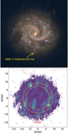 |
Fig. 3. Deprojected images of the host galaxy. Top panel: Deprojected false-color image of the galaxy using the HST and ALMA data using a PA of 110 deg and an inclination of 50 deg. The whitish dot at the outskirts of the lower spiral arm is the GRB-SN also indicated in Fig. 2. Bottom panel: Deprojected specific SFR, obtained from Hα and the HST UV continuum. Overplotted is the ring which contains most of the SF regions in the host, with exception of the GRB site (diamond) and some SF regions at the southern end of the bar (see also Sect. 6.3). |
4. Two-dimensional properties of the host
4.1. Star formation rate
We determine the current star formation rate (SFR) from the Hα flux according to Kennicutt (1992) assuming a Salpeter initial mass function (IMF) leading to a conversion of SFR = 7.2 × 10−42 LHα. The result is plotted in Fig. 4 showing the 2D map and the values at the deprojected distance from the center. We also obtain a map of the luminosity weighted specific SFR (sSFR/L), where the SFR is multiplied with the ratio between the absolute B-band magnitude and the magnitude of an L⋆ galaxy MB = −21 mag (Christensen et al. 2004):
 (1)
(1)
 |
Fig. 4. Maps and deprojected properties of SFR, metallicity and N/O. Top row: SFR from Hα. Second row: Luminosity-weighted SFR map and deprojected specific SFR from Hα. Third row: Metallicity using the O3N2 parameter (Marino et al. 2013) and deprojected values, fitted with a linear gradient of −0.009 dex/kpc. Fourth row: Map and deprojected plot of the N/O abundance derived from the N2S2 parameter. The star marks the value for a region of 2 × 2 spaxels at the GRB site, the red encircled H II region marks the one of the GRB. |
As B-band magnitude, we use the HST F475W filter image from the observations in Dec. 2019, which is similar in wavelength coverage to a B-band filter (see Fig. 4). The HST images from December 2019, which likely do not have any contamination from the GRB-SN any more, clearly show a small underlying SF region at the exact location of the GRB. Another, somewhat brighter SF region, lies to the south of it (see Fig. 2).
Ongoing star formation is present in most of the host galaxies; however, the highest values of both absolute and specific SFR are found in several H II regions distributed in a ring-like shape around the galaxy center, between ∼5 kpc and ∼7 kpc from the center, slightly closer to the center than the region of the GRB (see Figs. 3 and 4). The absolute SFR at the GRB site is slightly above the average value at that deprojected distance; however, the size of its SF region is small (∼300 pc in diameter), compared to other SF regions in the host. The total SFR of the galaxy derived from Hα is 2.28 ± 0.05 M⊙ yr−1. The sSFR/L at the exact GRB location has a value of 3.1 M⊙ yr−1 (L/L*)−1, the sSFR/L of the total H II region in which the GRB is located is slightly higher with 3.5 M⊙ yr−1 (L/L*)−1, which puts it among the highest 10% in of all H II regions in the galaxy. We will elaborate further on this in the discussion.
The high sSFR does not reflect in the global luminosity of the GRB H II region. Taking the results of the fractional flux analysis detailed in Sect. 3.1.2, the GRB region is among the 45% brightest pixel in UV (F300X), but in the 80% brightest pixels in F606W, which includes the Hα emission line (see Fig. A.5). Most studies on the fractional flux use HST data that are at restframe UV wavelengths, due to the higher average redshift of GRB hosts, corresponding to our observations in the F300X filter. Compared to previous studies (Kelly et al. 2008; Svensson et al. 2010; Blanchard et al. 2016; Lyman et al. 2017) the GRB site here is not a particularly bright region at wavelengths dominated by emission from massive stars. This might be explained by the unusual type of host galaxy for this GRB, where the GRB site was only one of several highly star-forming regions, while in the more common irregular hosts the GRB is more likely to be found in one of the few luminous star-forming regions.
4.2. Metallicity and N/O abundance
We determine the metallicity from emission lines using different strong emission line ratios. The direct Te method (Peimbert 1967) cannot be applied here as the temperature sensitive [O III] λ4363 line is only detected at a low S/N in a few regions of the host. Instead we use the O3N2 and N2 parameters in the reparametrization of Marino et al. (2013) based on the CALIFA sample of low redshift galaxies.
The O3N2 parameter shows a smooth negative metallicity gradient with no particular features. We fit the metallicity vs. distance with a simple linear fit and obtain a gradient of −0.015 dex kpc−1, which is shallow compared to other local disk galaxies (see e.g., Sánchez et al. 2014; Bresolin 2019) and does not show any flattening as observed in some of them. The metallicity in the GRB H II region is slightly lower than the average metallicity at that distance from the center (the typical metallicity error of the integrated H II regions is ∼0.01 dex), the GRB spaxel itself is consistent with the metallicity grandient. The N2 metallicity map shows a lower metallicity in the strong SF regions on top of the metallicity gradient (see Fig. A.4). In the past it has been pointed out that the N2 parameter depends on the ionization, which can affect the results (Schady et al. 2015) and, in fact, the regions of low metallicity clearly correlate with regions of high ionization (see next section). The O3N2 parameter handles the ionization issue somewhat better and, as shown in Fig. 4, the resulting metallicity map is smooth and shows no low metallicity regions specifically in the bright SF regions While the absolute value of the metallicity can depend on the metallicity calibrator used, the relative calibrations between different regions and spaxels, however, are reliable.
To further investigate the abundances in the host we plot the ratio of N/O (see Fig. 4), derived from the N2S2 parameter (N2S2 = log10([N II] λ6585/[S II] λ6714,6731) as originally introduced by Pilyugin et al. (2004), Mollá et al. (2006). We cannot determine the oxygen abundance directly since [O II] λλ3727,3729 is not in the range of the MUSE spectrum. Metal-poor, highly star-forming galaxies such as extreme emission line galaxies (EELGs) show an overabundance of nitrogen vs. oxygen compared to the general population of star-forming galaxies in the SDSS (Amorín et al. 2015). The reason for this could be WR stars, low-metallicity intermediate stars or inflows and outflows, but is likely linked to young stellar populations. The host of GRB171205A does not show a high ratio of N/O like EELGs (see Fig. 5). The different spaxels in the host, in fact, follow very closely the N/O versus metallicity correlation of SDSS SF galaxies. The regions of higher N/O ratio follow the inner spiral arms, and the ratio is highest in the bar, in particular at the end of the bar S-E of the center. The N/O abundance ratio at the GRB site is very similar to what is expected at this metallicity; however, looking at the entire H II region of the GRB, the value is one of the lowest in the host (see Fig. 4).
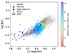 |
Fig. 5. N/O abundance vs. metallicity determined by the O3N2 parameter for different spaxels in the host of GRB171205A color coded according to distance from the center. The values are compared to star-forming galaxies in the SDSS (gray grid) and a sample of EELGs from Amorín et al. (2015). EELG metallicities were mostly determined using the Te method (Amorín et al. 2015), while for the SDSS galaxies we used the same O3N2 calibration as for the spaxels in the host. |
4.3. Extinction
In Fig. 6 we plot the 2D extinction map and the radial distribution of the extinction, derived from the Balmer decrement using Hα and Hβ, which, in the Case B recombination and zero extinction have an intrinsic ratio of 2.76 (Osterbrock & Ferland 2006). The color excess in most regions is low or even zero with a mean of 0.20 ± 0.17 mag. The highest extinction is observed in the center of the galaxy, which has E(B − V) = 1.3 mag. The location and H II region of the GRB does not show any extinction in the MUSE cube but shows some extinction in the late X-Shooter spectrum (see Table 3). The regions of highest extinction correlate very well with the CO emitting regions, which again correlate with the inter-arm regions and dust along the spiral arm (see Fig. 3).
Properties from the integrated spectra of different regions.
We furthermore derive an extinction from NaD absorption using the Voronoi binned cube, according to the relation between the NaD EW and E(B − V) established in Poznanski et al. (2012). The distribution follows a similar pattern with higher extinction in the center, but with overall higher values; however the relation between NaD EW and extinction has larger uncertainties than the Balmer decrement. The correlation with CO emission is less clear due to the lower spatial resolution used for this analysis. Again, the GRB region shows zero extinction. Finally, we derive an extinction map using the stellar population fitting described in the next section (see Fig. 6). Here we get again higher values in the core and zero extinction at the GRB site. Some of the young SF regions (see Sect. 4.6) in the spiral arms also show high extinction.
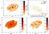 |
Fig. 6. Maps and deprojected properties of the extinction in the host, derived from different measurements. Top panels: E(B − V) determined from the Balmer decrement after correcting Hα and Hβ for stellar absorption. Bottom left panel: Extinction map using the correlation between the NaD EW and extinction from Poznanski et al. (2012). Bottom right panel: Extinction map from the stellar population fitting. The maps at the bottom were obtained from the Voronoi binned cube; the white region is a bin affected by a foreground star and has been omitted. Overplotted contours are derived from the ALMA CO(1−0) map (see de Ugarte Postigo et al. 2024). |
4.4. Ionization
Star-formation regions usually also show a high ionization level due to the strong UV radiation field from massive stars. The ratio of [O III] λ5008 versus Hα shows a clear slope of increasing [O III] toward the outer regions of the host: the GRB region and site are among the highest in the galaxy (see Fig. 7). However, [O III] is almost always weaker than Hα, in contrast to more extreme galaxies such as EELGs (e.g., Amorín et al. 2015).
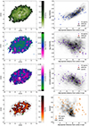 |
Fig. 7. Maps and deprojected properties of ionization measurements across the host. First row: [O III] λ5008 Å vs. Hα. Second row: Ionization of the ISM probed by [O I]/[O III]. Third row: Ionization parameter U derived from [S II]/Hβ and the O3N2 metallicity according to Díaz & Pérez-Montero (2000). Fourth row: He Iλ5876 vs. Hβ. |
We cannot determine directly the ionization of oxygen using [O II] λλ3727,29 since those doublet lines are outside the wavelength range of MUSE. The ratio [O I]/[O III] decreases with distance from the center of the galaxy (meaning that ionization increases) and the GRB H II region is in line with this trend. Here, however, the outer H II regions particularly stand out as more ionized regions, while the [O III]/Hα distribution is more smooth.
We also determine the ionization from the dimensionless parameter U based on the emission lines of [S II], Hβ and the metallicity (Díaz & Pérez-Montero 2000). The ionization parameter follows a similar pattern towards increasing ionization (lower U parameter) towards the outer regions of the host, but somewhat less pronounced as from the [O I]/[O III] ratio. The least ionized region is the H II region at the southern end of the bar, which also shows up as outlier in the [O III]/Hα map. Again, the H II regions in the outer part of the galaxy show a higher ionization and there is higher ionization along the western spiral arm extending from the end of the bar at the highly ionized region. The GRB region does not stand out as a particularly ionized region using this parameter.
He Iλ5876/Hβ can be used as indication for the hardness of the radiation field caused by either massive stars or another ionizing source. Usual values for galaxies such as the Magellanic Clouds show ratios of ∼0.03 (Martin & Kennicutt 1997). He I is also an indication of a young stellar population (González Delgado et al. 1999). Photoionization models give values of ∼0.13 during the first 5 Myr of a starburst. Our 2D map shows ratios around 0.15 in the inner regions of the regions with higher SF and especially along the spiral arm extending to the west, similar to what is observed in the U-parameter. He I around the GRB site shows a few higher value pixels, but here the extraction is complicated by the underlying supernova. The values are generally higher at the edges of the spiral arms, which could indicate some mildly shocked regions from the ISM driven away from the star-forming regions along the spiral arms.
4.5. Shocks
As a proxy for shocked regions we use the ratio of [S II]/Hα, plotted in Fig. 8, where strong [S II] indicate possible shocks. The high values at the edge of the galaxy are likely artefacts. Most of the strong star-forming regions show low values of [S II]/Hα while moderate values can be observed in the inter-arm regions. The highest values are observed in a region at the northwestern end of the bar and might actually be a signature of shocked gas induced by movements along the bar.
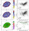 |
Fig. 8. Maps and deprojected properties of [O I]/Hα, [S II]/Hα and the Hα EW. First row: [O I]/Hα. Second row: log10 [S II]/Hα, indicative of shocked regions. Third row: Hα EW, the EW at the GRB site is only a lower limit due to the contamination of the continuum by the GRB-SN. The dashed line indicates the cut in EW applied to account for possible emission from diffuse ionized gas (see Sect. 6.1). |
No similar signature is observed at the S-E end of the bar, which contains the low ionized region mentioned in the previous subsection. The GRB region shows average values except for a few patches of higher values in the last inter-arm region east of the GRB site, while the spaxels around the GRB site show relatively high values, but not a larger pattern indicative of shocks. These observations, together with the kinematic analysis (see Sect. 5) do not point to an ongoing, violent shock or interaction scenario as an origin for the star formation in the GRB region.
A similar patter is observed for the ratio of [O I]/Hα, which is also indicative of shocks (Bik et al. 2018), with a median around −1.0, a scatter ∼0.5 dex and a slight increase towards the outer regions of the host. Regions with log([O I]/Hα) larger than ∼−1.0 could be regions excited by AGN activity; however, this seems unlikely in this galaxy and even the central H II region is below −1.0. A BPT diagram (Baldwin, Philips & Terlevich diagram, Baldwin et al. 1981) using [N II]/Hα (see Fig. 9) does not show any indication for AGN excitation anywhere in the galaxy.
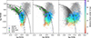 |
Fig. 9. BPT diagrams using [N II]/Hα, [S II]/Hα and [O I]/Hα for individual spaxels compared to the values for other long GRB hosts (green dots) and star forming galaxies in the SDSS (gray grid). The spaxels are color coded by their deprojected distance from the galaxy center as shown in the color bar. The value of the GRB site (color coded by its distance) is shown as a diamond. Emission lines for the GRB sample have been obtained from the same data used in Fig. 18. We only plot spaxels with EW < −6 Å to remove diffuse interstellar gas (DIG) as explained in the text. |
4.6. Star-formation history and stellar population age
In Fig. 10 we show the spectra of different regions in the host together with the result of the stellar population (SP) fit performed, as described in Section 3.2.2. For the integrated spectrum of the galaxy the residuals of the fit are very good with < 1%. This stellar population fit returns an average extinction of AV = 0.34 mag. Both the mass and the light fraction show a dominant population at around 900 Myr with additional contributions from older stars, but also a significant population with ages below 100 Myr and even some under 10 Myr, indicating recent SF activity.
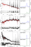 |
Fig. 10. Stellar population fits of different representative spectra. Top panel: Combined spectrum of the host. Middle panel: integrated spectrum of the core. Bottom panel: GRB site using the X-shooter observations from 14 months after the GRB instead of the SN contaminated MUSE spectra. In each panel, the top left box shows the observed spectrum (black) with the fitted spectrum overplotted in red, the lower left panel the residuals of the fit. The boxes on the right show the light (top) and mass (bottom) fraction for SPs at different ages. |
The spectrum from the core reveals a population dominated by old stars, but still with a contribution of a few percent to the light by younger stars in the 100 Myr range. This region has also a larger than average extinction of AV = 0.89 mag. To study the GRB region, we use the late time X-shooter spectrum from ∼14 months after the GRB where the contamination from the SN is negligible. We do detect some broad features, mainly at 5000−6000 Å which could be Fe-lines from the SN or residuals from the overlap between UVB and VIS arm, and which we hence exclude before fitting the stellar continuum. The H II region next to the GRB site, in the original cube, has a very blue continuum from the younger stars and a lower extinction of AV = 0.26 mag. Using the data derived from the stellar population fit, we then make maps in Voronoi binning corresponding to the age distribution in three different age ranges (Fig. 11).
 |
Fig. 11. Maps of the light percentage of the stellar population, divided into three age bins: the light percentage of the population < 30 Myr, the intermediate-age population of 30 Myr–1 Gyr, and the old population of > 1 Gyr. The white region in all three plots is a Voronoi bin affected by a foreground star and was therefore excluded from the analysis. |
The SP fit at the GRB site shows an older population of ∼1 Gyr contributing almost all of the stellar mass, and another peak with a very young population of only a few Myr contributing to the light but not the mass of the region. The GRB region has a contribution of ∼30% from a SP < 3 Myr, but 60% of the light comes from a SP of ∼1 Gyr, possibly from the last major SF event of the galaxy. Two H II regions show a light fraction for the youngest SP bin of > 60%. These regions as well as the GRB region show a small fraction of an intermediate population and a negligible contribution from a SP of > 1 Gyr. The other two young regions, however, are located at the opposite side of the galaxy compared to the GRB and within the SF “ring”, while the GRB region lies at a larger distance. This confirms that, indeed, there has been a recent onset of SF at the GRB site, which has produced the massive GRB progenitor. We will have a closer look at the other three young regions in Sect. 6.
Another, less direct, method to determine the age of the dominant stellar population is to measure the equivalent width (EW) of Hα, that is, the line luminosity compared to the continuum. Some of the other bright star-forming regions in the SF ring of the host show rather high EWs between −60 and −80 Å, which corresponds to a population age of ∼8−10 Myr according to STARBURST99 models at half solar metallicity6 (Leitherer et al. 1999). The EW at the GRB site from the MUSE cube is very low, with ∼−14 Å; however, this is only a lower limit due to the presence of the SN. For the GRB site we therefore measure the EW from the late time X-shooter spectrum, also used for the SP analysis described above. Despite the absence of the SN continuum, the EW remains low with only ∼ − 18 Å, not indicating a particularly young SP age. This probably results from the significant light contribution of an older stellar population at the site mentioned above.
5. Kinematic analysis
The kinematics of different states of the gas can give clues to possible star formation triggers such as gas inflows or past mergers or interactions. The rich dataset for this host allows us to analyze the velocity and dispersion maps of the ionized gas by probing Hα, the molecular gas via CO emission and the stellar kinematics using NaD absorption lines as well as investigate the environment for possible interacting neighbour galaxies.
5.1. The galactic environment of the host
The large field of view (FOV) of MUSE allows us to search for nearby galaxies at the same redshift. In the HST image there are several elongated objects and a round, low-surface brightness structure with a bright center at the north of the host. There is also a prominent object consisting of several bright knots ∼6 arcsec east-southeast of the host, which at first glance could be a satellite of the host galaxy. We checked for emission lines in all those objects and conclude that none of them are at the redshift of the GRB (see Fig. A.6). All objects described above belong to two groups of galaxies at z = 0.61 and z = 0.62, including the bright knots to the east-southeast, which hence is clearly not a satellite galaxy. The fact that most of the galaxies in those groups are edge on is an observational bias since edge-on galaxies are more easily detectable than face-on objects due to their higher apparent surface brightness.
Our observations in H I revealed another object at a similar redshift as the GRB (de Ugarte Postigo et al. 2024), a large H I disk from another spiral galaxy at a projected physical distance of 183 kpc to the northwest with a velocity difference of only ∼30 km s−1 (see Fig. A.7). As comparison, the LMC and SMC are located at 50 and 62 kpc, the Andromeda galaxy is at 770 kpc from the Milky Way. The companion has an H I mass similar to the host (log M = 9.45 M⊙ and 9.49 M⊙ for the host and companion, respectively) and shows a somewhat more regular H I disk than the host (see Fig. 12). We do not detect any H I gas between the two galaxies, which, if present, would likely be too faint to be detected in our data. As calculated in de Ugarte Postigo et al. (2024), assuming a transverse velocity between those two galaxies of ∼200 km s−1, the last encounter of the two galaxies happened 900 Myr ago, making an influence on the current SF of the host unlikely; however, we have no information no the actual relative velocity between the two objects.
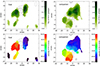 |
Fig. 12. Moment 0 and 1 maps of the host and companion observed in HI with VLA. Overlaid both objects are r′-band contours from PanSTARRS. Left: Moment 0 and 1 maps of the host galaxy. The ellipse in the top figure indicates the beam size. Right: Same for the distant companion galaxy. We note that the FOV here is larger than for the MUSE plots. |
The distant companion galaxy is also a spiral galaxy, albeit looking more irregular and with some bright star-forming regions. Unfortunately, no high resolution imaging of that galaxy is available to further study its morphology. Our PMAS data do not have a high enough S/N to allow for a detailed analysis and we only obtain resolved maps of Hα and [O III] (see Fig. A.8). Hβ is too weak and [N II] is almost not detected (the value listed in Table 2 is rather an upper limit than a detection). The outer spiral arms are very weak in Hα and we note that the [O III] emission in stronger in the S-E part, while Hα is more uniform. The metallicity of the galaxy is similar to the host of GRB 171205A (12 + log(O/H) = 8.47), but it has a considerably lower SFR of only 0.11 M⊙ yr−1 and also a very low Hα EW, and therefore no indication of a very young stellar population. The two galaxies are clearly part of a group, but their evolutionary paths are likely different.
5.2. Ionized gas kinematics
The ionized gas kinematics is traced using the Hα emission lines in the MUSE cube. In Fig. 13 we show the velocity and dispersion obtained from fitting a single Gaussian to Hα. Zero velocity is determined as the velocity at the brightest spaxel at the center of the host. The dispersion map is corrected for the instrumental resolution of MUSE, R ∼ 3000 at λ6600 Å. At first sight, the velocity field appears like a regular rotating disk. The dispersion map only shows a larger dispersion in the center due to the larger amount of material in the bulge and otherwise has values around 20−30 km s−1 with slightly higher velocities in the arms and somewhat lower in the interarm regions.
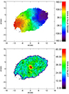 |
Fig. 13. Velocity and dispersion derived from a single Gaussian fit to the Hα line. The dispersion was corrected for the instrumental resolution of R ∼ 3000. |
To further analyze the kinematics, we fit kinemetry models (Krajnović et al. 2006) to the velocity field. This technique extracts the velocity profiles along ellipses around the center of the galaxy (as we assume disks are intrinsically round and appear as ellipses because of the inclination), which can be described by harmonic terms in Fourier analysis. The method looks for the best fitting ellipses to minimize those terms, which again then yield the parameters for these ellipses as a function of distance from the center of rotation. Fig. 14 shows the kinematic position angle (PA), the flattening of the ellipse q and the kinematic moments k1 and k1/k5 as a function of deprojected distance. The PA traces the position of maximum velocity, and therefore the PA of the best fit ellipses, q is related to the inclination by q = sin(i) and k1 as the first kinematic moment corresponding to the rotation curve of the galaxy. k5 traces the higher-order deviations from simple rotation and hence deviations from simple rotation. The kinematic center of the galaxy (v = 0 km s−1) is the brightest spaxel of Hα in the center, and corresponds to a redshift of z = 0.03714. The kinemetry code Krajnović et al. (2006) is then run for all ellipses with a minimum covering fraction of velocities of 0.7. No limits are given on q or PA.
 |
Fig. 14. Results from the kinemetry fit described in the text. Parameters obtained from the kinemetry analysis (Krajnović et al. 2006) (top). The PA of the fitted ellipses, their ellipticity q (second panel), k1 (third panel) is the first kinematic moment (equivalent to the rotation curve) and k5/k1 (fourth panel) the deviation from simple rotation. |
Figure 14 shows that the galaxy has a rotation curve (parameter k1) with a steep, linear, component out to ∼1.5 kpc after which it follows a smooth behavior out to the maximum distance where we can fit the Hα line. This is indeed the textbook behavior for a bar (which behaves as a solid body) and disk galaxy (rising and then flat rotation curve). In the same inner 1.5 kpc the ellipticity changes somewhat erratically with a sudden jump at 1.5 kpc and there are some deviations in the PA. The deviations k5/k1 from simple rotation is in general small but shows some higher values in the central 2 kpc, likely associated with the influence of the bar. At the end of the bar beyond ∼2 kpc the velocity field becomes much more regular, although some enhanced k5/k1 is present out to 4 kpc, possibly due to some remaining influence of the bar. A further increase in k5/k1 at the outermost part of the galaxy is likely a simple issue of S/N and coverage of the best fitting ellipse with the velocity data from Hα. For the same reason, the analysis does not allow to claim that the rotation curve actually starts to decline in the outermost part.
5.3. Molecular gas kinematics
The molecular gas traced by CO(1−0) emission has been presented in de Ugarte Postigo et al. (2024). Due to the much sparser velocity field probed by the CO emission we cannot do a full kinemetry analysis for the molecular gas, instead, we compare the Hα emission to the CO velocity map (see Fig. 15).
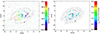 |
Fig. 15. CO velocity map (left) and residuals compared to the Hα velocity field (right). Contours are from the late-time HST F475W image. The GRB site is marked by a +. |
The velocity differences are < 15 km s−1 except the regions at the end of the bar/onset of the inner spiral arms, which show residuals up to ∼ − 50 km s−1. Disk galaxies have often higher rotation velocities for CO gas than for Hα (see e.g., Levy et al. 2018) with typical residuals of ∼25 km s−1, associated with extraplanar diffuse gas or a thick disk. At redshifts > 1 there are both examples of similar CO and Hα rotation curves and some with large discrepancies (Übler et al. 2018; Girard et al. 2019). Dispersions are often found to be larger for Hα like we observe in the host of GRB 171205A. In general, the gas dispersion in a galaxy seems to increase with redshift (Übler et al. 2019).
The largest residuals are measured at the northern end of the bar, the same region that shows indications of shocked material (see Sect. 4.5). The negative residuals could be an indication of an inflow of gas, as it is commonly observed in barred galaxies (see e.g., Yu et al. 2022, and references therein). Observations of galaxies in the local Universe have revealed details on gas transport and kinematics, especially in central regions and around the bar (see e.g., a study on M83 Della Bruna et al. 2022). Comparing the line width of Hα (see Fig. 13 and de Ugarte Postigo et al. 2024), there is a similar pattern with a high dispersion in the center and lower width in the spiral arms; however, both values are ∼15 km s−1 higher for Hα. There is no detection of CO at the GRB site itself, preventing further analysis of the gas content or kinematics of molecular gas in this part of the galaxy.
Only about 15 GRB hosts have to date been detected in CO using different transitions of CO (Stanway et al. 2015; Michalowski et al. 2018; Arabsalmani et al. 2018; Hatsukade et al. 2020; de Ugarte Postigo et al. 2020). Kinematical analysis has been limited to very rough velocity maps (Hatsukade et al. 2020), but often the only information is the CO line width due to the faintness of the emission. de Ugarte Postigo et al. (2020) make a comparison between the width of the CO line and Hβ in the host of GRB 190114C and find a very similar value. Arabsalmani et al. (2020) have CO(2−1) observations at comparable resolution for the much closer host of GRB 980425 at dL ∼ 38 Mpc, but not presenting a kinematic analysis of the full galaxy. Even for field galaxies, detailed 2D studies comparing ionized and molecular gas kinematics have been limited to galaxies in the local Universe such as the THINGS/SINGS/metal-THINGS survey (Kennicutt et al. 2003; Walter et al. 2008; Lara-López et al. 2023) and PHANGS survey (e.g., Leroy et al. 2021; Emsellem et al. 2022), only now being extended to higher redshifts by e.g., the CALIFA/EDGES survey (e.g., Levy et al. 2018).
5.4. Neutral gas kinematics
We rereduced the JVLA data already described in Arabsalmani et al. (2022) and analyze both the host and the companion in H I, the latter of which is not mentioned in Arabsalmani et al. (2022). Figure 12 shows the moment 0 (flux) and moment 1 (velocity) maps for both galaxies. As mentioned in de Ugarte Postigo et al. (2024), the companion has a higher total H I flux and also its spatial distribution is larger. Both galaxies have a velocity field of a rotating disk with a gap in the center of the disk and a slightly asymetric distribution with more HI gas in one half of the galaxy. Arabsalmani et al. (2022) found an extra component to the south of the GRB position (below the western lobe) in the VLA data, which we cannot recover in our rereduction of the same data. Instead, there seems to be a cloud offset south of the eastern lobe.
We used the high resolution JVLA data to analyze the kinematics of the H I gas and compare it to the ionized and molecular gas (see Fig. 16). The model velocity field used here is: v = v0 tanh(r/h) sin(i) cos(ϕ − PAk), where v is the line-of-sight velocity, r is the radius with respect to the center of the galaxy, ϕ is the angle with respect to the positive y-axis, PAk is the kinematic position angle of the galaxy, i is the inclination of the galaxy, and v0 and h are constants constrained by the true rotation velocity. This model has been used before to create mock galaxy velocity fields in Stark et al. (2018) and is similar to the two-parameter arctan function described in Courteau (1997) that has been used to describe galaxy rotation curves. A warp can be introduced to this model by changing the PAk with radius at a specific rate. This acts as an additional parameter in the model.
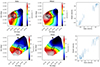 |
Fig. 16. Velocity fits to the host (top) and companion (bottom) as described in the text. Dotted values are regions of measured flux, overlaid are contours from PanSTARRS images as in Fig. 12. |
We fit the inclination, PAk, v0, h and the warp using the spatial and velocity data obtained from the JVLA observations. After a best-fit model is found, we calculate the normalized root mean squared error (NRMSE) to estimate how well the model fits the data. The NRMSE for the GRB 171205A host and companion are 0.073 and 0.078, respectively. While this fit does not exclude past interactions, it shows that the observed gas velocity can be described by the model used here. It also does not support the conclusions reached by Arabsalmani et al. (2022) of a recent interaction with a smaller satellite, of which there is no trace in the optical data.
6. Discussion
6.1. The GRB site compared to the host properties
To check for the peculiarity (or lack of thereof) of the GRB H II region, we compare a number of properties derived in Sect. 3 to (1) the average properties of all spaxels in the galaxy and (2) the average properties of the ISM in a ring of ±1 kpc compared to the galactocentric distance of the GRB of ∼8 kpc. We determine the mean and standard deviation for each property in all spaxels with sufficient S/N in (a) the entire host (see also Table 3) and (b) in a bin of ±1 kpc around the deprojected distance of the GRB. We subsequently determine the deviation of the GRB site as (propGRB–propgal/1 kpc)/standdevgal/1 kpc (see Fig. 17). SFR/spaxel, ionization and Hα EW at the GRB site are rather similar to the global and local values, the latter is due to the fact that the GRB site shows a rather low EW for an actively star-forming region. The extinction is considerably lower as it is consistent with zero at the GRB site. The metallicity is > 1σ lower at the GRB site, the fact that the deviation is less compared to the global metallicity is due to the larger standard deviation taking all spaxels in the galaxy. The sSFR does not have a large deviation in σ owing to the large standard deviation for this value in the galaxy, on an absolute scale, the sSFR in the GRB H II region and site are twice the average in the galaxy. We also note that the global properties derived from the integrated galaxy spectrum match rather well with the average values of all spaxels.
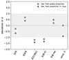 |
Fig. 17. Deviation in standard deviation σ of different properties in the GRB H II region compared to the mean value in the host (green diamonds) and compared to a bin of ±1 kpc around distance of the GRB (8 kpc, magenta dots). The SFR is determined as SFR/spaxel to account for the fact that the spectrum of the GRB HII region was integrated over several spaxels. |
We furthermore determine the position of the GRB site in the BPT diagram, the different spaxels in the galaxy as well as other long GRB hosts from the literature (see Fig. 9). BPT diagrams serve to distinguish regions excited by hot stars and those excited by AGN activity. In the most commonly used version, plotting [N II]/Hα vs. [O III]/Hβ do not show any indication for AGN excitation using the demarcation line of Kewley et al. (2007), but parts of the galaxy, including the GRB region, are in the intermediate region Kauffmann et al. (2003). The other two BPT diagrams using [S II]/Hα and [O I]/Hα do show parts of the galaxy, especially the outer regions, to fall into the AGN part. We also checked for a possible contribution from diffuse ionized gas (DIG), which can contribute several tens of % to the emission (see e.g., Poetrodjojo et al. 2019; Della Bruna et al. 2022). DIG is often found in interarm regions and is contributing a larger fraction in the outskirts of a galaxy. To remove a possible contribution from DIG we only plot spaxels with a Hα EW of < −6 Å. Applying this cut, we get a DIG fraction of 1.6%, which is low for a spiral galaxy, but possibly our S/N anyway removes most of the possible DIG contribution before any further analysis. Figure 8 shows that DIG might contribute a small part in the outskirts but almost nothing in the center of the galaxy. Hence we exclude DIG contributing significantly to the emission anywhere in the host. The values for individual spaxels show a trend from very low ionization regions in the center to values closer to the values for GRB hosts in the outskirts, including the GRB site. The GRB site has a relatively low ionization and high metallicity compared to those for other GRB hosts or sites, which are distributed more to the upper left of the diagram (Krühler et al. 2015). Only for the BPT diagram with [O I]/Hα do the values of the GRB site and galaxy fall in the same region as other long-GRB hosts; however, we only have [O I] clearly detected in four other GRB hosts. The high-ionization regions outside the photoionized regions in the [SII]/Hα and [OI]/Hα BPT diagrams are not due to extended amounts of DIG, we do not see any sign for AGN activity and most of the outlier spaxels are in the outskirts of the host, hence we attribute this high ionization as due to shocks.
There are two other regions in the host that have a very young stellar population, region 15 and 17 (for the H II region numbering and location, please refer to Fig. A.2) at the opposite side of the galaxy, with a higher fraction of a young population than the GRB site itself. Both regions have a moderate, but not very high sSFR and a metallicity at the host average. The lowest metallicity regions (20, 26 and 39, region 39 is next to the GRB site) do not show any particular pattern nor a very young stellar population and a lower sSFR than the GRB site. Several regions at the same side of the galaxy as the GRB (region 1, 4, 5 and 8) have both a high EWs and high sSFRs (> 3 M⊙ yr−1(L/L*)−1), the same is the case for regions 3 and 7 on the opposite, northern side of the galaxy. Moreover, region 3 has the highest values both in sSFR (4.87 M⊙ yr−1(L/L*)−1) and EW (−77 Å) and a metallicity on the lower side. The SP ages derived from STARBURST99 models, however, indicate SP ages of 7 Myr for the highest EW regions. Possibly several of these regions mentioned above might have also been able, in principle, to produce a GRB progenitor, but due to the scarcity of GRBs (GRBs are about 1/10 000 times less frequent than core-collapse SNe, see e.g., Spinelli & Ghirlanda 2023) and particularly rare in high-mass galaxies (Taggart & Perley 2021) it is unlikely to detect another GRB in the same galaxy. This scarcity might also point to some very peculiar stellar properties, that all have to occur in the same star, to actually make a star explode as a GRB, with many more parameters needing to be fulfilled than only the ISM properties from which the progenitor originates.
6.2. The GRB site and host in comparison to other GRB hosts
As a grand-design spiral, the host of GRB 171205A is a very rare type of GRB host. While it is difficult to determine the exact morphology of GRB hosts at higher redshifts, of the 47 long-GRB hosts at z < 0.5, there are only 10 confirmed spiral galaxies (including the host of GRB 171205A), which is ∼20%. However, two of them are disputed as being the actual host galaxy (GRB 190829A, a very large spiral host which might have a dwarf behind being the actual host, and GRB 051109B, where the host association is unclear), two are SN-less long GRBs (GRB 060505, a dwarf spiral, Thöne et al. 2014), and GRB 111005A, a nearly edge-on large spiral, Michalowski et al. 2018) and for GRB 011121 fits to the images suggest a disk and bulge, but definite imaging is missing. This is somewhat surprising since 40% of low mass galaxies (log M < 9.5 M⊙) and 70% of high mass galaxies (log M > 9.5 M⊙) at z < 1 are spiral galaxies or classified as “disky”, while the fraction of spirals goes to almost zero at z ∼ 4 (see the recent JWST study by Jacobs et al. 2023). In Fig. A.1 we plot the GRB hosts mentioned above in relative physical size together with the dwarf irregular host of GRB 100416D and the smallest host detected, the host of GRB 060218 with an r50 of only 0.36 kpc (Lyman et al. 2017). The typical GRB host has an r50 and r80 of 1.7 ± 0.2 and 3.1 ± 0.4 kpc respectively (Lyman et al. 2017), while the r50 for the host of GRB 171205A is 4.54 kpc, more than twice the median for long GRB hosts.
Long GRBs usually have a small offset from their host, in contrast to short GRBs. Since most long GRB hosts are dwarfs, the absolute median offset is only 1.0−1.3 kpc depending on the sample used (Blanchard et al. 2016; Lyman et al. 2017). The absolute distance for the GRB site of GRB 171205A is 5.23 kpc, almost 5 times larger than the median offset of previous samples. However, due to the different physical sizes of GRB hosts, it is more instructive to use the offset normalized to r50. The site of GRB 171205A has a normalized offset of 1.15, which puts it among the 20% largest offsets for long GRB hosts (Blanchard et al. 2016; Lyman et al. 2017) (see Fig. A.5), on the upper end of values for the offset but still well within a standard GRB host.
To compare the host of GRB 171205A with the general population of long GRB hosts we collect properties of 54 long GRB hosts from the literature up to z ∼ 2.4 with an average redshift of 0.93 using global or integrated spectra of the host as well as 7 low redshift (z < 0.65) resolved GRB sites (IFU and longslit). We derive metallicities using the O3N2 parameter (using the calibration in Marino et al. 2013) (47 hosts), the specific SFR (39 hosts), stellar mass (38 hosts), extinction (47 hosts) and Hα EWs (16 hosts) of both the integrated spectra and the sample of resolved GRB locations (except for the stellar mass where we do not have measurements for the GRB site only), visualized as violin plots in Fig. 18 (for references to the different literature samples used see the figure caption).
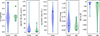 |
Fig. 18. Violin plots of different properties of global/integrated GRB host spectra (blue plots) and the same properties at the resolved GRB sites (green plots). The dots are the global values for the host of GRB 171205A, diamonds are the values at the GRB site of GRB 171205A. Emission lines for the integrated host spectra were obtained from the samples of Krühler et al. (2015), Han et al. (2010), with additional single GRBs from Della Valle et al. (2006), Christensen et al. (2008), Kelly et al. (2013), Schulze et al. (2014), Thöne et al. (2014), Izzo et al. (2017), Heintz et al. (2018), Cano et al. (2017b), de Ugarte Postigo et al. (2018, 2020), Melandri et al. (2019). Stellar masses were taken from the GHostS database (http://www.grbhosts.org) and Palmerio et al. (2019). Rest-frame B-band magnitudes to derive the sSFR were taken from the TOUGH sample (Hjorth et al. 2012) and Krühler et al. (2011). Hα EW were determined from public spectra stored in the GRBspec database (de Ugarte Postigo et al. 2014b). The values for the GRB sites were taken from Christensen et al. (2008), Thöne et al. (2014), Izzo et al. (2017), Cano et al. (2017b), de Ugarte Postigo et al. (2018), Melandri et al. (2019). |
Both the host and GRB site of GRB 171205A show a high metallicity compared to other GRB hosts/sites, the GRB site would even fall in the upper metallicity range for the global sample. We note that we derived all metallicities consistently using the O3N2 parameter in the calibration from Marino et al. (2013), which gives lower values than some of the calibrators used in, for example, Krühler et al. (2015) and we do not obtain any super solar values for the same GRB hosts in their study. The location in the BPT diagram at the lower end of the distribution for GRB hosts, implying a low ionization and high metallicity, is in line with this observation. Regarding the sSFR, the GRB site is somewhat above the median while the value of the integrated galaxy value falls below the median of the sample, not surprising given that the host is not a starburst galaxy. The mass of the galaxy is in the upper third of the distribution but not among the most massive hosts, which, however, are all at redshifts of z > 1, in line with the findings of Palmerio et al. (2019) that GRB host masses increase with redshift. Previous studies found a metallicity threshold for GRB hosts (Perley et al. 2016; Vergani et al. 2017; Schulze et al. 2014); however, this threashold was determined to be rather high (0.5−0.9 Z⊙), which is not in tension with our findings. The extinction of the host is average and the GRB site has one of the lowest values of the sample, also not surprising given its location in a small, blue star-forming region in the outskirts of the galaxy.
6.3. Kinematics of neutral vs. molecular vs. ionized gas and possible star formation triggers
The velocity fields of ionized (traced by Hα), and molecular (traced by CO(1−0)) gas are surprisingly smooth and show no sign of any major interaction in the recent past. Interaction is known as one of the triggers of star formation, in particular outside of denser cluster regions. The only major companion at the same redshift is 183 kpc from the host and any possible interaction would have happened at timescales much beyond what is needed for a recent burst of star formation.
In contrast, the H I gas distribution is more asymmetric. Arabsalmani et al. (2022) publish a high resolution map of H I of the VLA data which shows a butterfly like shape and an extra component in the S-W. While the main double-lobe of H I gas is likely the normal H I disk of the host, the extra component was interpreted as the H I disk of a recently interacting satellite. Our reanalysis of the same dataset did not result in any extraplanar emission in the western lobe, instead, we observe some extra component south of the eastern lobe, but also at low significance. Thus we issue caution here in the overinterpretation of any extraplanar feature. The kinematics of both the component plotted in Arabsalmani et al. (2022) and the different one we found in our analysis are consistent with being a part of the rotating H I disk. We do not find any evidence for other emission in the MUSE cube for any of these proposed extraplanar components, neither in continuum nor Hα.
Star formation in the host is concentrated into a ring around 5−7 kpc from the center, somewhat closer to the center than the GRB site, corresponding to an undisturbed inside-out star formation process in this galaxy. However, in the S-E part of the galaxy, where the GRB exploded, there is enhanced star formation both in- and outside of the main ring (see Fig. 3). This could suggest that the H I inflow/small merger triggered some additional SF in this region of the galaxy. There are a few regions with high sSFR, low metallicity and low SP age at this side of the galaxy, region 4, 5 and 8 discussed in Sect. 6.1 as well as the GRB region. The most extreme H II regions, however, are at the opposite side of the galaxy, where, if the merger has been rather recent, this seems unlikely as the trigger of high SF in that opposite part of the galaxy.
Our comparison between neutral, molecular and ionized gas do not show any obvious indication for this proposed merger to be the needed SF trigger. Michałowski et al. (2012, 2015) have found large amounts of H I gas close to the GRB site in several GRB hosts and propose inflow of H I gas as possible SF trigger. Arabsalmani et al. (2019) found a ring-like structure in the host of GRB 980425 in H I and interpret this as remaining from a previous interaction with a dwarf galaxy. Inflow or interaction only visible in H I gas might also be at place here, but we still lack any evidence in other wavelengths or properties to confirm this theory.
7. Conclusions
In this paper, we present the most extensive resolved multiwavelength study of a long GRB host to date. We find GRB 171205A to be at a redshift of z = 0.036 or 163 Mpc using MUSE/VLT IFU spectroscopy, HST UV, and VIS imaging as well as ALMA CO(1−0) and H I 21 cm observations. The main conclusions from this extensive dataset can be summarized as follows:
-
The host is a grand-design spiral galaxy with a short bar, which is a rare type for long-GRB hosts, in particular at low redshift (< 20%), which are primarily irregular galaxies. In contrast, almost half of the known low-redshift galaxies have a disk morphology.
-
The host shows a smooth negative metallicity gradient of −0.015 dex kpc−1. The total SFR is not particularly high, with ∼1 M⊙ yr−1.
-
The GRB was located in a small star-forming region in an outer spiral arm at a deprojected distance of ∼8 kpc. The metallicity at the GRB site is around half solar and the absolute SFR is low; likewise, the region is only among the 45% brightest pixels in the host in UV light. However, given the size of the H II region, the luminosity-weighted sSFR is one of the highest in the host (3.5 M⊙ yr−1(L L*)−1) and is high compared to other GRB sites. SP modeling suggests a significant contribution from a very young stellar population. The region appears to be dust-free with zero extinction.
-
The GRB site is not a particularly unique site in the host. Several other H II regions show a similar combination of low metallicity, high sSFR, and young age. The H II region in which the GRB occurred shows the sixth highest sSFR and the fourth lowest metallicity, a comparison of the age is complicated by the presence of the underlying GRB-SN.
-
The velocity field of the ionized and molecular gas is very regular with only small deviations in the center, connected to the bar. The end of the bar shows some further evidence of shocked regions from optical emission line ratios. The width of CO is ∼15 km s−1 lower than that of Hα, but the velocity fields of CO and Hα match well.
-
The H I emission is different from ionized and molecular gas, with an excess to the southeast of the galaxy, which could be connected to an inflow of gas. This has also been observed in the past for several other GRB hosts, but not for the hosts of other types of SNe.
Our study shows that long GRBs can occur in many different types of (star-forming) galaxies, including a rather standard yet star-forming galaxy for its redshift, and that the conditions at the actual site are more important than general host properties. Previous resolved studies of GRB hosts also showed differences between the GRB site and the global host properties, although these differences were generally not extreme (Christensen et al. 2008; Krühler et al. 2017; Thöne et al. 2014; Izzo et al. 2017). The sample is still rather small, but it is likely that, the larger and more unusual the host is, the larger the deviations of the GRB site from the host properties. This would be in favor of the idea that GRBs require a set of very limited conditions, which can occur in different types of galaxies as long as some star-forming region has precisely the right conditions to form a GRB. On the other hand, the region hosting a GRB progenitor, especially in larger hosts, might not be a unique region; considering the scarcity of stars turning into a GRB at the end of their lives, this is difficult to verify for any given host galaxy.
We also note that the GRB studied here was a so-called low-luminosity GRB (ll-GRB), which can only be observed at low redshifts due to their faint afterglow. Therefore, the results for cosmological GRBs might be different. On the other hand, properties such as metallicity and SFR were less extreme in this host and its GRB site than found for other GRB hosts. Several studies have found GRB production to be stifled above a certain metallicity, ranging between half solar and solar metallicity (Schulze et al. 2015; Perley et al. 2016; Palmerio et al. 2019). Only one paper has investigated and found a noncorrelation between metallicity and GRB γ-ray emission (Levesque et al. 2010); however this was based on a sample of only 16 GRBs before 2010. There may be physical reasons for the fact that this GRB host and site had a relatively high metallicity while the GRB, afterglow, and SN were all relatively weak (which also made the detection of the cocoon emission possible); for example, it may be that higher-metallicity stars lead to an almost-choked jet. Further studies of this topic are warranted.
Despite the extensive dataset across the electromagnetic spectrum, the origin of the SF hosting this GRB is still unclear. Violent SF or a SF trigger through major interactions does not seem to be needed to produce a GRB progenitor, and there have been very few cases so far of any kind of recent interaction triggering new SF. However, several hosts do show an asymmetric, offset, extraplanar presence of H I gas, often close to the location of the GRB. Further highly detailed and panchromatic studies are needed to obtain adequate statistics on the kinematics of the different gas components, as well as abundances and other properties at the GRB site, and extension to higher redshifts is also highly warranted, albeit observationally challenging.
Data availability
The reduced JVLA datacube is available at the CDS via anonymous ftp to cdsarc.cds.unistra.fr (130.79.128.5) or via https://cdsarc.cds.unistra.fr/viz-bin/cat/J/A+A/690/A66
PI: N. Tanvir, Program ID 0100.D-0649.
CAHA project no. 19A-3.5-029, PI: L. Izzo.
For a complete description of the parameters, see: https://gitlab.com/SoFiA-Admin/SoFiA-2/-/wikis/SoFiA-2-Control-Parameters
Acknowledgments
Based on observations collected at the European Organisation for Astronomical Research in the Southern Hemisphere under ESO programme 0100.D-0649. JFAF acknowledges support from the Spanish Ministerio de Ciencia, Innovación y Universidades through the grant PRE2018-086507. M.J.M. acknowledges the support of the National Science Centre, Poland through the SONATA BIS grant 2018/30/E/ST9/00208 and the Polish National Agency for Academic Exchange Bekker grant BPN/BEK/2022/1/00110. AJL was supported by the European Research Council (ERC) under the European Union’s Horizon 2020 research and innovation programme (grant agreement No. 725246). L.C. is supported by DFF/Independent Research Fund Denmark, grant-ID 2032–00071. J.L. thanks Aaron Lawson and Ananthan Karunakaran for useful discussions regarding the VLA data. This research has made use of the GHostS database (www.grbhosts.org), which is partly funded by Spitzer/NASA grant RSA Agreement No. 1287913. This research is based on observations made with the NASA/ESA Hubble Space Telescope obtained from the Space Telescope Science Institute, which is operated by the Association of Universities for Research in Astronomy, Inc., under NASA contract NAS 5–26555. These observations are associated with program 15349.
References
- Amorín, R., Pérez-Montero, E., Contini, T., et al. 2015, A&A, 578, A105 [NASA ADS] [CrossRef] [EDP Sciences] [Google Scholar]
- Arabsalmani, M., Le Floc’h, E., Dannerbauer, H., et al. 2018, MNRAS, 476, 2332 [NASA ADS] [CrossRef] [Google Scholar]
- Arabsalmani, M., Roychowdhury, S., Starkenburg, T. K., et al. 2019, MNRAS, 485, 5411 [NASA ADS] [CrossRef] [Google Scholar]
- Arabsalmani, M., Renaud, F., Roychowdhury, S., et al. 2020, ApJ, 899, 165 [NASA ADS] [CrossRef] [Google Scholar]
- Arabsalmani, M., Roychowdhury, S., Renaud, F., et al. 2022, AJ, 164, 69 [NASA ADS] [CrossRef] [Google Scholar]
- Baldwin, J. A., Phillips, M. M., & Terlevich, R. 1981, PASP, 93, 5 [Google Scholar]
- Bik, A., Östlin, G., Menacho, V., et al. 2018, A&A, 619, A131 [NASA ADS] [CrossRef] [EDP Sciences] [Google Scholar]
- Blanchard, P. K., Berger, E., & Fong, W.-F. 2016, ApJ, 817, 144 [Google Scholar]
- Bresolin, F. 2019, MNRAS, 488, 3826 [NASA ADS] [Google Scholar]
- Bruzual, G., & Charlot, S. 2003, MNRAS, 344, 1000 [NASA ADS] [CrossRef] [Google Scholar]
- Calzetti, D., Armus, L., Bohlin, R. C., et al. 2000, ApJ, 533, 682 [NASA ADS] [CrossRef] [Google Scholar]
- Cano, Z., Wang, S.-Q., Dai, Z.-G., & Wu, X.-F. 2017a, Adv. Astron., 2017, 8929054 [CrossRef] [Google Scholar]
- Cano, Z., Izzo, L., de Ugarte Postigo, A., et al. 2017b, A&A, 605, A107 [NASA ADS] [CrossRef] [EDP Sciences] [Google Scholar]
- Cappellari, M., & Copin, Y. 2003, MNRAS, 342, 345 [Google Scholar]
- CASA Team (Bean, B., et al.) 2022, PASP, 134, 114501 [NASA ADS] [CrossRef] [Google Scholar]
- Chrimes, A. A., Stanway, E. R., & Eldridge, J. J. 2020, MNRAS, 491, 3479 [NASA ADS] [CrossRef] [Google Scholar]
- Christensen, L., Hjorth, J., & Gorosabel, J. 2004, A&A, 425, 913 [NASA ADS] [CrossRef] [EDP Sciences] [Google Scholar]
- Christensen, L., Vreeswijk, P. M., Sollerman, J., et al. 2008, A&A, 490, 45 [NASA ADS] [CrossRef] [EDP Sciences] [Google Scholar]
- Cid Fernandes, R., Mateus, A., Sodré, L., Stasińska, G., & Gomes, J. M. 2005, MNRAS, 358, 363 [Google Scholar]
- Cid Fernandes, R., Schoenell, W., Gomes, J. M., et al. 2009, Rev. Mex. Astron. Astrofis. Conf. Ser., 35, 127 [Google Scholar]
- Courteau, S. 1997, AJ, 114, 2402 [Google Scholar]
- Della Bruna, L., Adamo, A., McLeod, A. F., et al. 2022, A&A, 666, A29 [NASA ADS] [CrossRef] [EDP Sciences] [Google Scholar]
- Della Valle, M., Chincarini, G., Panagia, N., et al. 2006, Nature, 444, 1050 [NASA ADS] [CrossRef] [Google Scholar]
- Detmers, R. G., Langer, N., Podsiadlowski, P., & Izzard, R. G. 2008, A&A, 484, 831 [NASA ADS] [CrossRef] [EDP Sciences] [Google Scholar]
- de Ugarte Postigo, A., Thöne, C. C., Rowlinson, A., et al. 2014a, A&A, 563, A62 [NASA ADS] [CrossRef] [EDP Sciences] [Google Scholar]
- de Ugarte Postigo, A., Blazek, M., Janout, P., et al. 2014b, SPIE Conf. Ser., 9152, 91520B [NASA ADS] [Google Scholar]
- de Ugarte Postigo, A., Izzo, L., Kann, D. A., et al. 2017, GRB Coordinates Network, 22204 [Google Scholar]
- de Ugarte Postigo, A., Thöne, C. C., Bensch, K., et al. 2018, A&A, 620, A190 [NASA ADS] [CrossRef] [EDP Sciences] [Google Scholar]
- de Ugarte Postigo, A., Thöne, C. C., Martín, S., et al. 2020, A&A, 633, A68 [EDP Sciences] [Google Scholar]
- de Ugarte Postigo, A., Michalowski, M., Thoene, C. C., et al. 2024, A&A, submitted [arXiv:2406.16726] [Google Scholar]
- Díaz, A. I., & Pérez-Montero, E. 2000, MNRAS, 312, 130 [CrossRef] [Google Scholar]
- Dichiara, S., Bernardini, M. G., Burrows, D. N., et al. 2019, GRB Coordinates Network, 25552 [Google Scholar]
- Emsellem, E., Schinnerer, E., Santoro, F., et al. 2022, A&A, 659, A191 [NASA ADS] [CrossRef] [EDP Sciences] [Google Scholar]
- Fruchter, A. S., Levan, A. J., Strolger, L., et al. 2006, Nature, 441, 463 [NASA ADS] [CrossRef] [Google Scholar]
- Fynbo, J. P. U., Watson, D., Thöne, C. C., et al. 2006, Nature, 444, 1047 [NASA ADS] [CrossRef] [Google Scholar]
- Girard, M., Dessauges-Zavadsky, M., Combes, F., et al. 2019, A&A, 631, A91 [NASA ADS] [CrossRef] [EDP Sciences] [Google Scholar]
- González Delgado, R. M., Leitherer, C., & Heckman, T. M. 1999, ApJS, 125, 489 [CrossRef] [Google Scholar]
- Han, X. H., Hammer, F., Liang, Y. C., et al. 2010, A&A, 514, A24 [NASA ADS] [CrossRef] [EDP Sciences] [Google Scholar]
- Hatsukade, B., Ohta, K., Hashimoto, T., et al. 2020, ApJ, 892, 42 [NASA ADS] [CrossRef] [Google Scholar]
- Heintz, K. E., Malesani, D., Wiersema, K., et al. 2018, MNRAS, 474, 2738 [NASA ADS] [CrossRef] [Google Scholar]
- Hjorth, J., Sollerman, J., Møller, P., et al. 2003, Nature, 423, 847 [Google Scholar]
- Hjorth, J., Malesani, D., Jakobsson, P., et al. 2012, ApJ, 756, 187 [Google Scholar]
- Izzo, L., Thöne, C. C., Schulze, S., et al. 2017, MNRAS, 472, 4480 [Google Scholar]
- Izzo, L., de Ugarte Postigo, A., Maeda, K., et al. 2019, Nature, 565, 324 [Google Scholar]
- Jacobs, C., Glazebrook, K., Calabrò, A., et al. 2023, ApJ, 948, L13 [NASA ADS] [CrossRef] [Google Scholar]
- Jones, D. H., Read, M. A., Saunders, W., et al. 2009, MNRAS, 399, 683 [Google Scholar]
- Jones, A., Noll, S., Kausch, W., Szyszka, C., & Kimeswenger, S. 2013, A&A, 560, A91 [NASA ADS] [CrossRef] [EDP Sciences] [Google Scholar]
- Kauffmann, G., Heckman, T. M., Tremonti, C., et al. 2003, MNRAS, 346, 1055 [Google Scholar]
- Kelly, P. L., Kirshner, R. P., & Pahre, M. 2008, ApJ, 687, 1201 [NASA ADS] [CrossRef] [Google Scholar]
- Kelly, P. L., Filippenko, A. V., Fox, O. D., Zheng, W., & Clubb, K. I. 2013, ApJ, 775, L5 [NASA ADS] [CrossRef] [Google Scholar]
- Kennicutt, R. C. 1992, ApJ, 388, 310 [Google Scholar]
- Kennicutt, R. C., Armus, L., Bendo, G., et al. 2003, PASP, 115, 928 [NASA ADS] [CrossRef] [Google Scholar]
- Kent, B. R., Masters, J. S., Chandler, C. J., et al. 2020, ASP Conf. Ser., 527, 571 [NASA ADS] [Google Scholar]
- Kewley, L. J., Brown, W. R., Geller, M. J., Kenyon, S. J., & Kurtz, M. J. 2007, AJ, 133, 882 [NASA ADS] [CrossRef] [Google Scholar]
- Koribalski, B. S., Staveley-Smith, L., Westmeier, T., et al. 2020, Ap&SS, 365, 118 [Google Scholar]
- Krajnović, D., Cappellari, M., de Zeeuw, P. T., & Copin, Y. 2006, MNRAS, 366, 787 [Google Scholar]
- Krühler, T., Greiner, J., Schady, P., et al. 2011, A&A, 534, A108 [CrossRef] [EDP Sciences] [Google Scholar]
- Krühler, T., Malesani, D., Fynbo, J. P. U., et al. 2015, A&A, 581, A125 [Google Scholar]
- Krühler, T., Kuncarayakti, H., Schady, P., et al. 2017, A&A, 602, A85 [NASA ADS] [CrossRef] [EDP Sciences] [Google Scholar]
- Lara-López, M. A., Pilyugin, L. S., Zaragoza-Cardiel, J., et al. 2023, A&A, 669, A25 [NASA ADS] [CrossRef] [EDP Sciences] [Google Scholar]
- Leitherer, C., Schaerer, D., Goldader, J. D., et al. 1999, ApJS, 123, 3 [Google Scholar]
- Leroy, A. K., Schinnerer, E., Hughes, A., et al. 2021, ApJS, 257, 43 [NASA ADS] [CrossRef] [Google Scholar]
- Leung, J. K., Murphy, T., Ghirlanda, G., et al. 2021, MNRAS, 503, 1847 [NASA ADS] [CrossRef] [Google Scholar]
- Levan, A. J., Lyman, J. D., Tanvir, N. R., et al. 2017, ApJ, 848, L28 [Google Scholar]
- Levesque, E. M., Soderberg, A. M., Kewley, L. J., & Berger, E. 2010, ApJ, 725, 1337 [NASA ADS] [CrossRef] [Google Scholar]
- Levy, R. C., Bolatto, A. D., Teuben, P., et al. 2018, ApJ, 860, 92 [NASA ADS] [CrossRef] [Google Scholar]
- Liang, E., Zhang, B., Virgili, F., & Dai, Z. G. 2007, ApJ, 662, 1111 [NASA ADS] [CrossRef] [Google Scholar]
- Lyman, J. D., Levan, A. J., Tanvir, N. R., et al. 2017, MNRAS, 467, 1795 [NASA ADS] [Google Scholar]
- Marino, R. A., Rosales-Ortega, F. F., Sánchez, S. F., et al. 2013, A&A, 559, A114 [NASA ADS] [CrossRef] [EDP Sciences] [Google Scholar]
- Martin, C. L., & Kennicutt, R. C. 1997, ApJ, 483, 698 [CrossRef] [Google Scholar]
- McMullin, J. P., Waters, B., Schiebel, D., Young, W., & Golap, K. 2007, ASP Conf. Ser., 376, 127 [Google Scholar]
- Melandri, A., Malesani, D. B., Izzo, L., et al. 2019, MNRAS, 490, 5366 [Google Scholar]
- Michałowski, M. J., Kamble, A., Hjorth, J., et al. 2012, ApJ, 755, 85 [CrossRef] [Google Scholar]
- Michałowski, M. J., Gentile, G., Hjorth, J., et al. 2015, A&A, 582, A78 [NASA ADS] [CrossRef] [EDP Sciences] [Google Scholar]
- Michalowski, M. J., Xu, D., Stevens, J., et al. 2018, A&A, 616, A169 [CrossRef] [EDP Sciences] [Google Scholar]
- Modjaz, M., Liu, Y. Q., Bianco, F. B., & Graur, O. 2016, ApJ, 832, 108 [NASA ADS] [CrossRef] [Google Scholar]
- Modjaz, M., Bianco, F. B., Siwek, M., et al. 2020, ApJ, 892, 153 [NASA ADS] [CrossRef] [Google Scholar]
- Mollá, M., Vílchez, J. M., Gavilán, M., & Díaz, A. I. 2006, MNRAS, 372, 1069 [CrossRef] [Google Scholar]
- Nicuesa Guelbenzu, A. M., Klose, S., Schady, P., et al. 2021a, ApJ, 923, 38 [NASA ADS] [CrossRef] [Google Scholar]
- Nicuesa Guelbenzu, A. M., Klose, S., Schady, P., et al. 2021b, A&A, 650, A117 [NASA ADS] [CrossRef] [EDP Sciences] [Google Scholar]
- Noll, S., Kausch, W., Barden, M., et al. 2012, A&A, 543, A92 [NASA ADS] [CrossRef] [EDP Sciences] [Google Scholar]
- Osterbrock, D. E., & Ferland, G. J. 2006, Astrophysics of Gaseous Nebulae and Active Galactic Nuclei (Sausalito: University Science Books) [Google Scholar]
- Palmerio, J. T., Vergani, S. D., Salvaterra, R., et al. 2019, A&A, 623, A26 [NASA ADS] [CrossRef] [EDP Sciences] [Google Scholar]
- Patel, M., Gompertz, B. P., O’Brien, P. T., et al. 2023, MNRAS, 523, 4923 [NASA ADS] [CrossRef] [Google Scholar]
- Peimbert, M. 1967, ApJ, 150, 825 [NASA ADS] [CrossRef] [Google Scholar]
- Perley, D. A., Tanvir, N. R., Hjorth, J., et al. 2016, ApJ, 817, 8 [Google Scholar]
- Pilyugin, L. S., Vílchez, J. M., & Contini, T. 2004, A&A, 425, 849 [NASA ADS] [CrossRef] [EDP Sciences] [Google Scholar]
- Planck Collaboration VI. 2020, A&A, 641, A6 [NASA ADS] [CrossRef] [EDP Sciences] [Google Scholar]
- Poetrodjojo, H., D’Agostino, J. J., Groves, B., et al. 2019, MNRAS, 487, 79 [Google Scholar]
- Poznanski, D., Prochaska, J. X., & Bloom, J. S. 2012, MNRAS, 426, 1465 [Google Scholar]
- Rastinejad, J. C., Gompertz, B. P., Levan, A. J., et al. 2022, Nature, 612, 223 [NASA ADS] [CrossRef] [Google Scholar]
- Roth, M. M., Kelz, A., Fechner, T., et al. 2005, PASP, 117, 620 [Google Scholar]
- Sanchez, S. F. 2016, Astrophysics Source Code Library [record ascl:1603.017] [Google Scholar]
- Sánchez, S. F., Rosales-Ortega, F. F., Iglesias-Páramo, J., et al. 2014, A&A, 563, A49 [CrossRef] [EDP Sciences] [Google Scholar]
- Sandin, C., Becker, T., Roth, M. M., et al. 2010, A&A, 515, A35 [NASA ADS] [CrossRef] [EDP Sciences] [Google Scholar]
- Savaglio, S., Rau, A., Greiner, J., et al. 2012, MNRAS, 420, 627 [NASA ADS] [CrossRef] [Google Scholar]
- Schady, P., Krühler, T., Greiner, J., et al. 2015, A&A, 579, A126 [NASA ADS] [CrossRef] [EDP Sciences] [Google Scholar]
- Schady, P., Yates, R. M., Christensen, L., et al. 2024, MNRAS, 529, 2807 [NASA ADS] [CrossRef] [Google Scholar]
- Schlafly, E. F., & Finkbeiner, D. P. 2011, ApJ, 737, 103 [Google Scholar]
- Schlegel, D. J., Finkbeiner, D. P., & Davis, M. 1998, ApJ, 500, 525 [Google Scholar]
- Schneider, B., Le Floc’h, E., Arabsalmani, M., Vergani, S. D., & Palmerio, J. T. 2022, A&A, 666, A14 [NASA ADS] [CrossRef] [EDP Sciences] [Google Scholar]
- Schulze, S., Malesani, D., Cucchiara, A., et al. 2014, A&A, 566, A102 [NASA ADS] [CrossRef] [EDP Sciences] [Google Scholar]
- Schulze, S., Chapman, R., Hjorth, J., et al. 2015, ApJ, 808, 73 [NASA ADS] [CrossRef] [Google Scholar]
- Serra, P., Oosterloo, T., Morganti, R., et al. 2012, MNRAS, 422, 1835 [Google Scholar]
- Serra, P., Westmeier, T., Giese, N., et al. 2015, MNRAS, 448, 1922 [Google Scholar]
- Spinelli, R., & Ghirlanda, G. 2023, Universe, 9, 60 [NASA ADS] [CrossRef] [Google Scholar]
- Stanway, E. R., Levan, A. J., Tanvir, N. R., Wiersema, K., & van der Laan, T. P. R. 2015, ApJ, 798, L7 [Google Scholar]
- Stark, D. V., Bundy, K. A., Westfall, K., et al. 2018, MNRAS, 480, 2217 [NASA ADS] [CrossRef] [Google Scholar]
- Svensson, K. M., Levan, A. J., Tanvir, N. R., Fruchter, A. S., & Strolger, L.-G. 2010, MNRAS, 405, 57 [NASA ADS] [Google Scholar]
- Taggart, K., & Perley, D. A. 2021, MNRAS, 503, 3931 [NASA ADS] [CrossRef] [Google Scholar]
- Tanga, M., Krühler, T., Schady, P., et al. 2018, A&A, 615, A136 [NASA ADS] [CrossRef] [EDP Sciences] [Google Scholar]
- Thöne, C. C., Christensen, L., Prochaska, J. X., et al. 2014, MNRAS, 441, 2034 [Google Scholar]
- Thöne, C. C., Izzo, L., Flores, H., et al. 2021, A&A, 656, A136 [NASA ADS] [CrossRef] [EDP Sciences] [Google Scholar]
- Übler, H., Genzel, R., Tacconi, L. J., et al. 2018, ApJ, 854, L24 [CrossRef] [Google Scholar]
- Übler, H., Genzel, R., Wisnioski, E., et al. 2019, ApJ, 880, 48 [Google Scholar]
- van Moorsel, G., Kemball, A., & Greisen, E. 1996, ASP Conf. Ser., 101, 37 [NASA ADS] [Google Scholar]
- Vergani, S. D., Palmerio, J., Salvaterra, R., et al. 2017, A&A, 599, A120 [NASA ADS] [CrossRef] [EDP Sciences] [Google Scholar]
- Walter, F., Brinks, E., de Blok, W. J. G., et al. 2008, AJ, 136, 2563 [Google Scholar]
- Westmeier, T., Kitaeff, S., Pallot, D., et al. 2021, MNRAS, 506, 3962 [NASA ADS] [CrossRef] [Google Scholar]
- Woosley, S. E., & Heger, A. 2006, ApJ, 637, 914 [CrossRef] [Google Scholar]
- Yoon, S. C., Langer, N., & Norman, C. 2006, A&A, 460, 199 [NASA ADS] [CrossRef] [EDP Sciences] [Google Scholar]
- Yu, S.-Y., Kalinova, V., Colombo, D., et al. 2022, A&A, 666, A175 [NASA ADS] [CrossRef] [EDP Sciences] [Google Scholar]
Appendix A: Additional figures and tables
Properties of the integrated H II regions, region 33 contains the GRB
Table A.1. continued.
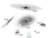 |
Fig. A.1. Comparison of the physical size of different low redshift long GRB hosts including the host of GRB 171205A. The red circles have a radius of 1 kpc and are placed at the best known location of each burst. Also indicated is the typical r50 = 1.7 kpc of long GRB hosts (Lyman et al. 2017). |
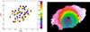 |
Fig. A.2. Left: H II regions with extracted integrated spectra used in the analysis throughout the paper. Overlaid are continuum contours from HST. We number the H II regions for easier reference in the text. Right: Voronoi tessellation of the MUSE continuum data constructed to give a S/N of 40 per bin. |
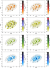 |
Fig. A.3. From top left to bottom left: Maps of Hα, Hβ, [O III] λ 5008, [O I] λ 6300, [N II] λ 6585, the sum of the [S II] λλ 6717,6732 doublet, He Iλ 5877 and Ar IIIλ 7135, all fluxes are 10−17 erg cm−2 Å−1 and corrected for Galactic and host intrinsic extinction. The position of the GRB is indicated with a black circle. |
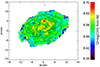 |
Fig. A.4. Map of the metallicity determined by the N2 parameter according to Marino et al. (2013). |
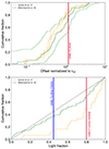 |
Fig. A.5. Top: Cumulative offsets normalized to r50 for two samples of long GRB hosts galaxies observed with HST (Lyman et al. 2017; Blanchard et al. 2016). The offset for GRB 171205A is the measured offset, not the deprojected offset used elsewhere in the paper since the comparison samples are mostly irregular galaxies where deprojection is hampered. Bottom: Cumulative distribution of the fraction of brightest pixel at the GRB site in different GRB host galaxies from the same sample as in the plot above. The dashed line indicates the GRB site following the general light distribution. The two lines indicate the light fraction for the site of GRB 171205A in the F300X filter (UV) and F606W filter (∼R-band). |
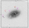 |
Fig. A.6. Galaxies in the FOV of MUSE around the host of GRB 171205A with their corresponding redshifts. None of the sources are physically related to the GRB host. |
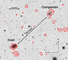 |
Fig. A.7. Larger view of the field including the host galaxy and the companion mentioned throughout the paper. Red contours are from VLA. Both objects are at a very similar redshift and hence part of a group. |
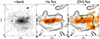 |
Fig. A.8. R-band image and emission line maps of Hα and [O III] λ 5008 for LEDA 951348, the galaxy companion of the host of GRB 171205A at 186 kpc. |
All Tables
Log of the observations used in this paper. The last column refers to the presence or absence of the underlying GRB-SN.
All Figures
|
Fig. 1. Integrated spectra and detected lines in (top to bottom): the integrated galaxy spectrum, the galaxy core and bar, the GRB region, and H II regions 15 and 17, which show a very young stellar population. |
| In the text | |
|
Fig. 2. Multi-color image of the host of GRB 171205A. Small panels, top left: False-color image based on HST images in filters F606W (red), F473W (green), and F300X (blue) taken in July 2018 with the GRB-SN still present. Center left: CO(1−0) emission from ALMA. Bottom left: H I emission from JVLA, including contours. Large panel: False-color image combining the HST data together with the CO(1−0) emission from ALMA (dark red) and H I emission from JVLA (white clouds). The inset shows data from December 2019 when the SN had faded and revealed the underlying star-forming region at the GRB site, marked by a green circle. In all images, north is up and east is left. |
| In the text | |
|
Fig. 3. Deprojected images of the host galaxy. Top panel: Deprojected false-color image of the galaxy using the HST and ALMA data using a PA of 110 deg and an inclination of 50 deg. The whitish dot at the outskirts of the lower spiral arm is the GRB-SN also indicated in Fig. 2. Bottom panel: Deprojected specific SFR, obtained from Hα and the HST UV continuum. Overplotted is the ring which contains most of the SF regions in the host, with exception of the GRB site (diamond) and some SF regions at the southern end of the bar (see also Sect. 6.3). |
| In the text | |
|
Fig. 4. Maps and deprojected properties of SFR, metallicity and N/O. Top row: SFR from Hα. Second row: Luminosity-weighted SFR map and deprojected specific SFR from Hα. Third row: Metallicity using the O3N2 parameter (Marino et al. 2013) and deprojected values, fitted with a linear gradient of −0.009 dex/kpc. Fourth row: Map and deprojected plot of the N/O abundance derived from the N2S2 parameter. The star marks the value for a region of 2 × 2 spaxels at the GRB site, the red encircled H II region marks the one of the GRB. |
| In the text | |
|
Fig. 5. N/O abundance vs. metallicity determined by the O3N2 parameter for different spaxels in the host of GRB171205A color coded according to distance from the center. The values are compared to star-forming galaxies in the SDSS (gray grid) and a sample of EELGs from Amorín et al. (2015). EELG metallicities were mostly determined using the Te method (Amorín et al. 2015), while for the SDSS galaxies we used the same O3N2 calibration as for the spaxels in the host. |
| In the text | |
|
Fig. 6. Maps and deprojected properties of the extinction in the host, derived from different measurements. Top panels: E(B − V) determined from the Balmer decrement after correcting Hα and Hβ for stellar absorption. Bottom left panel: Extinction map using the correlation between the NaD EW and extinction from Poznanski et al. (2012). Bottom right panel: Extinction map from the stellar population fitting. The maps at the bottom were obtained from the Voronoi binned cube; the white region is a bin affected by a foreground star and has been omitted. Overplotted contours are derived from the ALMA CO(1−0) map (see de Ugarte Postigo et al. 2024). |
| In the text | |
|
Fig. 7. Maps and deprojected properties of ionization measurements across the host. First row: [O III] λ5008 Å vs. Hα. Second row: Ionization of the ISM probed by [O I]/[O III]. Third row: Ionization parameter U derived from [S II]/Hβ and the O3N2 metallicity according to Díaz & Pérez-Montero (2000). Fourth row: He Iλ5876 vs. Hβ. |
| In the text | |
|
Fig. 8. Maps and deprojected properties of [O I]/Hα, [S II]/Hα and the Hα EW. First row: [O I]/Hα. Second row: log10 [S II]/Hα, indicative of shocked regions. Third row: Hα EW, the EW at the GRB site is only a lower limit due to the contamination of the continuum by the GRB-SN. The dashed line indicates the cut in EW applied to account for possible emission from diffuse ionized gas (see Sect. 6.1). |
| In the text | |
|
Fig. 9. BPT diagrams using [N II]/Hα, [S II]/Hα and [O I]/Hα for individual spaxels compared to the values for other long GRB hosts (green dots) and star forming galaxies in the SDSS (gray grid). The spaxels are color coded by their deprojected distance from the galaxy center as shown in the color bar. The value of the GRB site (color coded by its distance) is shown as a diamond. Emission lines for the GRB sample have been obtained from the same data used in Fig. 18. We only plot spaxels with EW < −6 Å to remove diffuse interstellar gas (DIG) as explained in the text. |
| In the text | |
|
Fig. 10. Stellar population fits of different representative spectra. Top panel: Combined spectrum of the host. Middle panel: integrated spectrum of the core. Bottom panel: GRB site using the X-shooter observations from 14 months after the GRB instead of the SN contaminated MUSE spectra. In each panel, the top left box shows the observed spectrum (black) with the fitted spectrum overplotted in red, the lower left panel the residuals of the fit. The boxes on the right show the light (top) and mass (bottom) fraction for SPs at different ages. |
| In the text | |
|
Fig. 11. Maps of the light percentage of the stellar population, divided into three age bins: the light percentage of the population < 30 Myr, the intermediate-age population of 30 Myr–1 Gyr, and the old population of > 1 Gyr. The white region in all three plots is a Voronoi bin affected by a foreground star and was therefore excluded from the analysis. |
| In the text | |
|
Fig. 12. Moment 0 and 1 maps of the host and companion observed in HI with VLA. Overlaid both objects are r′-band contours from PanSTARRS. Left: Moment 0 and 1 maps of the host galaxy. The ellipse in the top figure indicates the beam size. Right: Same for the distant companion galaxy. We note that the FOV here is larger than for the MUSE plots. |
| In the text | |
|
Fig. 13. Velocity and dispersion derived from a single Gaussian fit to the Hα line. The dispersion was corrected for the instrumental resolution of R ∼ 3000. |
| In the text | |
|
Fig. 14. Results from the kinemetry fit described in the text. Parameters obtained from the kinemetry analysis (Krajnović et al. 2006) (top). The PA of the fitted ellipses, their ellipticity q (second panel), k1 (third panel) is the first kinematic moment (equivalent to the rotation curve) and k5/k1 (fourth panel) the deviation from simple rotation. |
| In the text | |
|
Fig. 15. CO velocity map (left) and residuals compared to the Hα velocity field (right). Contours are from the late-time HST F475W image. The GRB site is marked by a +. |
| In the text | |
|
Fig. 16. Velocity fits to the host (top) and companion (bottom) as described in the text. Dotted values are regions of measured flux, overlaid are contours from PanSTARRS images as in Fig. 12. |
| In the text | |
|
Fig. 17. Deviation in standard deviation σ of different properties in the GRB H II region compared to the mean value in the host (green diamonds) and compared to a bin of ±1 kpc around distance of the GRB (8 kpc, magenta dots). The SFR is determined as SFR/spaxel to account for the fact that the spectrum of the GRB HII region was integrated over several spaxels. |
| In the text | |
|
Fig. 18. Violin plots of different properties of global/integrated GRB host spectra (blue plots) and the same properties at the resolved GRB sites (green plots). The dots are the global values for the host of GRB 171205A, diamonds are the values at the GRB site of GRB 171205A. Emission lines for the integrated host spectra were obtained from the samples of Krühler et al. (2015), Han et al. (2010), with additional single GRBs from Della Valle et al. (2006), Christensen et al. (2008), Kelly et al. (2013), Schulze et al. (2014), Thöne et al. (2014), Izzo et al. (2017), Heintz et al. (2018), Cano et al. (2017b), de Ugarte Postigo et al. (2018, 2020), Melandri et al. (2019). Stellar masses were taken from the GHostS database (http://www.grbhosts.org) and Palmerio et al. (2019). Rest-frame B-band magnitudes to derive the sSFR were taken from the TOUGH sample (Hjorth et al. 2012) and Krühler et al. (2011). Hα EW were determined from public spectra stored in the GRBspec database (de Ugarte Postigo et al. 2014b). The values for the GRB sites were taken from Christensen et al. (2008), Thöne et al. (2014), Izzo et al. (2017), Cano et al. (2017b), de Ugarte Postigo et al. (2018), Melandri et al. (2019). |
| In the text | |
|
Fig. A.1. Comparison of the physical size of different low redshift long GRB hosts including the host of GRB 171205A. The red circles have a radius of 1 kpc and are placed at the best known location of each burst. Also indicated is the typical r50 = 1.7 kpc of long GRB hosts (Lyman et al. 2017). |
| In the text | |
|
Fig. A.2. Left: H II regions with extracted integrated spectra used in the analysis throughout the paper. Overlaid are continuum contours from HST. We number the H II regions for easier reference in the text. Right: Voronoi tessellation of the MUSE continuum data constructed to give a S/N of 40 per bin. |
| In the text | |
|
Fig. A.3. From top left to bottom left: Maps of Hα, Hβ, [O III] λ 5008, [O I] λ 6300, [N II] λ 6585, the sum of the [S II] λλ 6717,6732 doublet, He Iλ 5877 and Ar IIIλ 7135, all fluxes are 10−17 erg cm−2 Å−1 and corrected for Galactic and host intrinsic extinction. The position of the GRB is indicated with a black circle. |
| In the text | |
|
Fig. A.4. Map of the metallicity determined by the N2 parameter according to Marino et al. (2013). |
| In the text | |
|
Fig. A.5. Top: Cumulative offsets normalized to r50 for two samples of long GRB hosts galaxies observed with HST (Lyman et al. 2017; Blanchard et al. 2016). The offset for GRB 171205A is the measured offset, not the deprojected offset used elsewhere in the paper since the comparison samples are mostly irregular galaxies where deprojection is hampered. Bottom: Cumulative distribution of the fraction of brightest pixel at the GRB site in different GRB host galaxies from the same sample as in the plot above. The dashed line indicates the GRB site following the general light distribution. The two lines indicate the light fraction for the site of GRB 171205A in the F300X filter (UV) and F606W filter (∼R-band). |
| In the text | |
|
Fig. A.6. Galaxies in the FOV of MUSE around the host of GRB 171205A with their corresponding redshifts. None of the sources are physically related to the GRB host. |
| In the text | |
|
Fig. A.7. Larger view of the field including the host galaxy and the companion mentioned throughout the paper. Red contours are from VLA. Both objects are at a very similar redshift and hence part of a group. |
| In the text | |
|
Fig. A.8. R-band image and emission line maps of Hα and [O III] λ 5008 for LEDA 951348, the galaxy companion of the host of GRB 171205A at 186 kpc. |
| In the text | |
Current usage metrics show cumulative count of Article Views (full-text article views including HTML views, PDF and ePub downloads, according to the available data) and Abstracts Views on Vision4Press platform.
Data correspond to usage on the plateform after 2015. The current usage metrics is available 48-96 hours after online publication and is updated daily on week days.
Initial download of the metrics may take a while.