| Issue |
A&A
Volume 689, September 2024
|
|
|---|---|---|
| Article Number | A248 | |
| Number of page(s) | 21 | |
| Section | Interstellar and circumstellar matter | |
| DOI | https://doi.org/10.1051/0004-6361/202450736 | |
| Published online | 19 September 2024 | |
SO2 and OCS toward high-mass protostars
A comparative study of ice and gas
1
Laboratory for Astrophysics, Leiden Observatory, Leiden University,
PO Box 9513,
2300
RA
Leiden,
The Netherlands
2
Leiden Observatory, Leiden University,
PO Box 9513,
2300
RA
Leiden,
The Netherlands
3
European Southern Observatory,
Garching,
Germany
4
Max-Planck-Institut für Extraterrestrische Physik,
Giessenbachstrasse 1,
85748
Garching,
Germany
Received:
16
May
2024
Accepted:
17
July
2024
Abstract
Context. OCS and SO2 are both major carriers of gaseous sulfur and are the only sulfurated molecules detected in interstellar ices to date. They are thus the ideal candidates for exploring the evolution of the volatile sulfur content throughout the different stages of star formation.
Aims. We aim to investigate the chemical history of interstellar OCS and SO2 by deriving a statistically significant sample of gas-phase column densities toward massive protostars and comparing them to observations of gas and ices toward other sources, from dark clouds to comets.
Methods. We analyzed a subset of 26 line-rich massive protostars observed by ALMA in Band 6 as part of the High Mass Protocluster Formation in the Galaxy (ALMAGAL) survey. Column densities were derived for OCS and SO2 from their rare isotopologs O13CS and 34SO2 toward the compact gas around the hot cores. We compared the abundance ratios of gaseous OCS, SO2, and CH3OH with ice detections toward both high- and low-mass sources as well as dark clouds and comets.
Results. We find that gas-phase column density ratios of OCS and SO2 with respect to methanol remain fairly constant as a function of luminosity between low- and high-mass sources, despite their very different physical conditions. In our dataset, OCS and SO2 are weakly correlated. The derived gaseous OCS and SO2 abundances relative to CH3OH are overall similar to protostellar ice values, with a significantly larger scatter for SO2 than for OCS. Cometary and dark-cloud ice values agree well with protostellar gas-phase ratios for OCS, whereas higher abundances of SO2 are generally seen in comets compared to the other sources. Gaseous SO2/OCS ratios are consistent with ices toward dark clouds, protostars, and comets, albeit with some scatter.
Conclusions. The constant gas-phase column density ratios throughout low- and high-mass sources indicate an early-stage formation before intense environmental differentiation begins. Icy protostellar values are similar to the gas-phase medians and are compatible with an icy origin for these species followed by thermal sublimation. The larger spread in SO2 compared to OCS ratios with respect to CH3OH is likely due to a more water-rich chemical environment associated with the former, as opposed to a CO-rich origin for the latter. Post-sublimation gas-phase processing of SO2 can also contribute to the large spread. Comparisons to ices in dark clouds and comets point to a significant inheritance of OCS from earlier to later evolutionary stages.
Key words: astrochemistry / techniques: interferometric / stars: protostars / ISM: abundances / ISM: molecules
Corresponding author; This email address is being protected from spambots. You need JavaScript enabled to view it.
© The Authors 2024
 Open Access article, published by EDP Sciences, under the terms of the Creative Commons Attribution License (https://creativecommons.org/licenses/by/4.0), which permits unrestricted use, distribution, and reproduction in any medium, provided the original work is properly cited.
This article is published in open access under the Subscribe to Open model. This email address is being protected from spambots. You need JavaScript enabled to view it. to support open access publication.
1 Introduction
Over 240 molecules have been detected in the interstellar medium to date, among which at least 30 contain one or more sulfur atoms (McGuire 2022). With an abundance of S/H ~ 1.35 × 10⁻⁵, sulfur is one of the most common elements in space (Asplund et al. 2009). S-bearing species are observed in the gas phase throughout most stages of star and planet formation, from diffuse and dense clouds (e.g., Drdla et al. 1989; Navarro-Almaida et al. 2020; Spezzano et al. 2022; Esplugues et al. 2022) and protostars (e.g., Blake et al. 1987, 1994; van der Tak et al. 2003; Li et al. 2015; Drozdovskaya et al. 2018; Codella et al. 2021; Artur de la Villarmois et al. 2023; Fontani et al. 2023; Kushwahaa et al. 2023) to protoplanetary disks (Fuente et al. 2010; Phuong et al. 2018; Semenov et al. 2018; Le Gal et al. 2019, 2021; Rivière-Marichalar et al. 2021; Booth et al. 2024). They have also been detected in Solar System bodies such as comets (Smith et al. 1980; Bockelée-Morvan et al. 2000; Biver et al. 2021a,b; Calmonte et al. 2016; Altwegg et al. 2022), planets (Moullet et al. 2013), and satellites (Hibbitts et al. 2000; Jessup et al. 2007; Moullet et al. 2008; Cartwright et al. 2020), as well as toward extragalactic sources (Henkel & Bally 1985; Petuchowski & Bennett 1992; Mauersberger et al. 1995; Heikkilä et al. 1999; Martín et al. 2003, 2005). Identified species range from simple diatomic molecules such as CS and SO to the complex organics methanethiol and ethanethiol (CH3SH and CH3CH2SH; Linke et al. 1979; Gibb et al. 2000; Cernicharo et al. 2012; Kolesniková et al. 2014; Zapata et al. 2015; Müller et al. 2016; Majumdar et al. 2016; Rodríguez-Almeida et al. 2021).
Despite this widespread detection, derived abundances in dense starless cores, protostars, and protoplanetary disks can only account for up to a few percent of the total expected cosmic value (Tieftrunk et al. 1994; Wakelam et al. 2004; Anderson et al. 2013; Vastel et al. 2018; Fuente et al. 2019, 2023; Le Gal et al. 2019, 2021; Rivière-Marichalar et al. 2019, 2020; Bouscasse et al. 2022). The bulk of the sulfur content is largely thought to be locked away in or underneath the ice mantles that shroud interstellar dust grains, in a state that makes its detection challenging. Such icy mantles start to form early in the interstellar evolutionary sequence, during the so-called translucent-cloud phase. Atoms of H and O adsorb onto dust grains and react to form H2O, resulting in a water-rich ice layer (Tielens & Hagen 1982; Hiraoka et al. 1998; Mokrane et al. 2009; Dulieu et al. 2010; Ioppolo et al. 2010; Cuppen et al. 2010; Romanzin et al. 2011; Öberg et al. 2011). As the density of the collapsing cloud increases, carbon monoxide (CO) molecules present in the gas phase catastrophically freeze out on top of the water-rich ice, forming a second coating known as the CO-rich ice layer (Tielens et al. 1991; Boogert et al. 2002; Pontoppidan et al. 2003; Pontoppidan 2006; Öberg et al. 2011). This CO ice is efficiently converted into methanol (CH3OH) by reactions involving H atoms (Tielens & Hagen 1982; Charnley et al. 1992; Hiraoka et al. 1994; Watanabe & Kouchi 2002; Fuchs et al. 2009; Cuppen et al. 2009; Santos et al. 2022). Complementarily, some smaller contribution to CH3OH formation from ice chemistry in less dense environments, before the catastrophic CO freeze-out, is also often invoked (e.g., Wada et al. 2006; Hodyss et al. 2009; Öberg et al. 2010; Bergner et al. 2017; Lamberts et al. 2017; Qasim et al. 2018), although it is likely not dominant.
Eventually, the environment close to the emerging young stellar object is warmed up to temperatures of 100–300 K, resulting in the complete thermal sublimation of the ices. This chemically rich region surrounding the protostar is known as the hot core for massive sources or the hot corino for low-mass counterparts (e.g., Herbst & van Dishoeck 2009), and is thought to be representative of the bulk ice content. For simplicity, we henceforth utilize “hot core” as an umbrella term for both high- and low-mass sources. By studying the compact emission originated from the hot core in comparison to ice observations, it is possible to gain insight into the formation and destruction mechanisms of molecules in both the gas and solid phases.
Compared to gaseous species, the unambiguous detection of solid-state molecules embedded in interstellar ices poses significantly more challenges. Spectral features of species in the solid phase are intrinsically broad and highly degenerate, with properties such as peak position and width that vary considerably with the ice environment. Likely as a consequence of such inherent limitations, only two sulfur-bearing species have been identified in ices so far: carbonyl sulfide (OCS) and sulfur dioxide (SO2). The former was first detected by Palumbo et al. (1995) toward the massive protostar W33A. Soon after, Boogert et al. (1997) suggested the presence of the latter toward both W33A and NGC 7538:IRS1 – another massive young stellar object (MYSO). Since then, both species have been either inferred or detected in ices toward other protostars as well as dark clouds (Palumbo et al. 1997; Öberg et al. 2008; Zasowski et al. 2009; Yang et al. 2022; Boogert et al. 2022; McClure et al. 2023; Rocha et al. 2024). Recently, the presence of SO2 ice was confirmed by James Webb Space Telescope (JWST) observations toward the solar-type protostar IRAS 2A by constraining the contribution of blended species, in particular OCN−, to its 7.6 μm region (Rocha et al. 2024).
In the gas phase, both species are commonly detected. Gaseous SO2 is observed toward protostellar systems both through its pure rotational transitions occurring at submillimeter wavelengths and through its rovibrational lines probed by the mid-infrared (Keane et al. 2001; Dungee et al. 2018; Nickerson et al. 2023; van Gelder et al. 2024). It is a good tracer of outflows, jets, and accretion shocks due to its enhanced gas-phase formation at high temperatures (T ≳ 100 K) combined with either sputtering or thermal sublimation of SO2 or its precursors from icy dust grains (Pineau des Forêts et al. 1993; Sakai et al. 2014; Oya et al. 2019; Taquet et al. 2020; Tychoniec et al. 2021; van Gelder et al. 2021). It has also been shown to trace disk winds (Tabone et al. 2017). While this is the case for the main isotopolog (i.e., 32SO2), the emission of minor isotopologs such as 34SO2 is expected to be mostly compact, tracing the hot core region. Moreover, in contrast to SO2, gaseous OCS emission is not expected to have significant contributions from outflows (van der Tak et al. 2003; Drozdovskaya et al. 2018), tracing predominately the envelope surrounding protostars (e.g., Herpin et al. 2009; Oya et al. 2016). As the only two sulfurated molecules detected in both gas and ices, SO2 and OCS are the ideal targets for performing a comparative study between these two physical states.
In this work, we explored the origin and fate of two of the most abundant sulfur species, OCS and SO2, by directly comparing their solid and gaseous components during the evolution of star-forming regions. We utilized data from the ALMA Evolutionary study of High Mass Protocluster Formation in the Galaxy (ALMAGAL) survey and selected a subsample of 26 line-rich sources to perform the analysis. This is the first interferometric study on a statistically significant sample of detections for these two molecules in the gas phase. The molecular column densities were derived from the rare isotopologs O13CS and 34SO2 to avoid contamination from extended emission and to limit line optical depth effects. We thus focused on the hot core region, which contains the molecular reservoir from the ices after complete thermal sublimation. We compared their ratios to other observations in the solid and gas phases taken from the literature. This includes recent work that utilized ground-based infrared observatories to investigate OCS ice abundances (among other species) in a large sample of MYSOs (Boogert et al. 2022), as well as space observations by JWST of both OCS and SO2 ices toward sources ranging from background stars to protostars (McClure et al. 2023; Rocha et al. 2024). This work sets the stage for future studies of gas and ice enabled by the combination of data from the Atacama Large Millimeter/submillimeter Array (ALMA) and JWST on both low- and high-mass protostars, paving the way to a more thorough understanding of the sulfur chemical evolution of the interstellar medium.
In Sec. 2, we describe the observational parameters and details of the dataset, as well as the procedure for fitting a synthetic spectrum to the lines of interest. The resulting emission morphologies, kinematics, and column densities are presented in Sec. 3. The column density ratios with respect to methanol and in comparison to other observations are discussed in Sec. 4. Finally, our main findings and conclusions are summarized in Sec. 5.
2 Observations and methods
2.1 The observations
The ALMAGAL survey (2019.1.00195.L; PIs: P. Schilke, S. Molinari, C. Battersby, P. Ho) was observed by ALMA in Band 6 (~1 mm). It targeted over 1000 dense clumps across the Galaxy with M > 500 M⊙ and d < 7.5 kpc, chosen based on the Herschel infrared Galactic Plane Survey (Hi-GAL; Molinari et al. 2010; Elia et al. 2017, 2021). ALMAGAL covers a statistically significant sample of sources in all stages of star formation, with many of them consisting of MYSOs. For this work we considered only archival data made publicly available before February 2021 and with beam sizes between 0.5″ and 1.5″ (~1000–5000 au). The Common Astronomy Software Applications1 (CASA; McMullin et al. 2007) version 5.6.1. was used to pipeline calibrate and image the data. The selection of sources was based on a subset studied in both Nazari et al. (2022) and van Gelder et al. (2022a), thus culling for particularly line-rich sources for which the CH3OH column densities – our benchmark for comparison – are well constrained. In van Gelder et al. (2022a), the selection was based on sources with high bolometric luminosities (Lbol > 1000 L⊙) where complex organic molecules such as CH3OH and CH3CN were detected. In Nazari et al. (2022), the selection criterium consisted of sources that contain the CH3CN 127−117 line above the 2.5–3σ level. Within the subset studied by both Nazari et al. (2022) and van Gelder et al. (2022a), we excluded sources for which the line profiles of the targeted molecules differed significantly across species, to avoid probing distinct emitting regions. An example case of an excluded source is shown in Appendix A. The final subset consists of 26 line-rich sources, whose properties and observational parameters are listed in Appendix B.
In this work, we made use of two out of the four spectral windows in ALMAGAL, encompassing frequencies of ~217.00–218.87 GHz and ~219.07–220.95 GHz with a spectral resolution of ~0.5 MHz (~0.7 km s−1). The spectral windows cover 4 transitions of 34SO2, 11 transitions of 33SO2, and 1 transition of O13CS with upper energy Eup < 800 K and Einstein Aij > 1 × 10⁻⁶ s−1 (see Appendix C). However, only the 111,11−100,10 transitions of 34SO2 and 33SO2 were detected in our sources (Eup = 60.1 K and 57.9 K, respectively). For 34SO2, this corresponds to only one line, whereas for 33SO2 it encompasses 7 hyperfine components caused by the nuclear spin I = 3/2 of the 33S atom. The remaining 34SO2 and 33SO2 lines are rather weak (Aij < 2.6 × 10⁻⁵ s−1) and for the most part highly blended, hampering their detections. O13CS is detected in its 18–17 transition (Eup = 99.5 K). No other isotopologs of OCS, including O12CS, are covered in the ALMAGAL range. One line of 32SO2 is covered, but it is not included in this work due to its likely contamination from outflow emission and because it is probably optically thick.
The spectra utilized in this work are the same as in van Gelder et al. (2022a). For all sources with the CH3OH 80,8−71,6 line (Eup = 97 K) above the 3σ level, the spectra were extracted from the peak pixel for this line in the integrated intensity maps. This particular transition of CH3OH was chosen because it is the strongest methanol line within the sample with Eup > 70 K, to avoid contamination by the outflow or extended emission that are probed by lines with lower Eup. The choice of extracting the spectra from the methanol peak intends to maximize the signal-to-noise ratio of both 34SO2 and O13CS originating from the hot core region. In G023.3891p00.1851, the peak emission of the methanol isotopolog CH2DOH is offset by ~0.6″ (approximately half a beam) from that of CH3OH, and thus the CH2DOH 171,16e0−170,17e0 (Eup = 336 K) peak is chosen to extract the spectrum since it is a more reliable tracer of the hot core. All sources probed here show line widths of ≳3 km s−1, well above the spectral resolution of ~0.7 km s−1, and the spectral sensitivity corresponds to ~0.2 K (for a list of rms values see Appendix B).
2.2 Spectral analysis
The target molecules of this study are SO2 and OCS, the two sulfur-bearing species detected in both gas and ices so far. We analyzed them by means of their rare isotopologs 34SO2 and O13CS in order to avoid issues with optically thick lines and contamination from extended emission and outflows. The 33SO2 emission is also analyzed as a diagnostic tool to assess whether or not 34SO2 is indeed optically thin (Sec. 3.3). We utilized the CASSIS2 spectral analysis tool (Vastel et al. 2015) to fit the spectrum for each source and derive each species’ column density (N) and full width at half maximum (FWHM) assuming that the excitation is under local thermodynamic equilibrium. Since we only detect one line per species per source, the excitation temperature was fixed to Tex = 150 K in the spectral fittings – a roughly averaged value for hot cores (see, e.g., van Gelder et al. 2020; Yang et al. 2021; Nazari et al. 2022). Fixing the Tex to 60–250 K only changes the derived column densities by up to a factor of ~3, and both molecules in the same direction. Furthermore, for ≳80% of the sources in this work, excitation temperatures derived from CH3CN lines range between 120 and 170 K (Nazari et al. 2022), corresponding to only up to a factor of 1.6 difference in column densities for SO2 and OCS. Thus, the assumption of a fixed Tex = 150 K does not interfere significantly with the column density ratios – the main focus of this work. The spectroscopic properties employed in the fittings of each species are obtained from the Cologne Database for Molecular Spectroscopy (CDMS; Müller et al. 2001, 2005).
The 34SO2 and O13CS lines analyzed in this work are mostly unblended, which allows the utilization of the grid fitting method as explained in detail previously (van Gelder et al. 2020; Nazari et al. 2021; Chen et al. 2023). In summary, a grid of column densities and FWHMs is tested and the best-fit model is assigned to the combination with the lowest χ2. In this work N was varied from 1 × 1013 cm−2 to 1 × 1017 cm−2 with a step of 0.1 on a logarithmic scale, and the FWHM was varied from 3 km s−1 to 11 km s−1 with a spacing of 0.1 km s−1 on a linear scale. The radial velocities (Vlsr) are derived by eye using increments of 0.1 km s−1 in a similar manner as described in Nazari et al. (2022) and Chen et al. (2023), and are fixed to the best manually derived values for the grid fits. Their median offsets are of 0.35 km s−1 from the velocities for CH3OH in the same sources (see Sec. 3.2). The 2σ errors are derived from the reduced χ2 calculated from the comparison between the resulting model of each grid point and the observed spectrum. If the 2σ uncertainties of the column densities are smaller than 20%, we assumed a 20% uncertainty as a conservative estimate to account for systematic sources of errors. In a few instances, such as for 34SO2 in 693050, more severe blending or deviations from a Gaussian profile are observed (see Appendix D). Nonetheless, the integrated line emissions are still encompassed by our models well within the adopted conservative uncertainties, and thus it does not affect our analysis. In the cases of G025.6498p01.0491 for 34SO2, and 126348 and 707948 for O13CS, the emission is better described by two components (see Appendix D). However, obtaining column density ratios for each velocity component separately is not possible since they are not resolved for methanol. In such cases, we performed the grid fits assuming one Gaussian and fixing the Vlsr to the mean between the values derived by eye for each component. This procedure yields column densities within 20% of the ones obtained by manually fitting each component separately. Thus, to ensure a systematic approach to the line analysis, we utilized the column densities derived from the grid fittings to these sources. The exact source sizes are not known, so we assumed that the source fully fills the beam (i.e., a beam dilution factor of unity). Since this work focuses on comparing column density ratios, this assumption does not interfere with the analysis as long as the lines are optically thin (van Gelder et al. 2020; Nazari et al. 2021).
Fitting 33SO2 is more challenging. It is considerably less abundant than 34SO2, and its only detected transitions are blended with ![Mathematical equation: $\[\mathrm{CH}_3^{13} \mathrm{CN}\]$](/articles/aa/full_html/2024/09/aa50736-24/aa50736-24-eq1.png) . The fitting was thus performed by eye on top of the best models for
. The fitting was thus performed by eye on top of the best models for ![Mathematical equation: $\[\mathrm{CH}_3^{13} \mathrm{CN}\]$](/articles/aa/full_html/2024/09/aa50736-24/aa50736-24-eq2.png) derived by Nazari et al. (2022). The Vlsr values of 33SO2 were fixed to those of 34SO2, while its column densities and FWHMs were varied in steps of 0.1 in log space and 0.1 in linear space, respectively. For most sources, barely or no emission was left underfit after accounting for
derived by Nazari et al. (2022). The Vlsr values of 33SO2 were fixed to those of 34SO2, while its column densities and FWHMs were varied in steps of 0.1 in log space and 0.1 in linear space, respectively. For most sources, barely or no emission was left underfit after accounting for ![Mathematical equation: $\[\mathrm{CH}_3^{13} \mathrm{CN}\]$](/articles/aa/full_html/2024/09/aa50736-24/aa50736-24-eq3.png) . In such cases we assigned 33SO2 as upper limits. However, for four sources (615590, 644284A, 693050, and G343.1261-00.0623) the
. In such cases we assigned 33SO2 as upper limits. However, for four sources (615590, 644284A, 693050, and G343.1261-00.0623) the ![Mathematical equation: $\[\mathrm{CH}_3^{13} \mathrm{CN}\]$](/articles/aa/full_html/2024/09/aa50736-24/aa50736-24-eq4.png) model underfit the emission significantly (≲50%), in which cases we could derive approximate column densities for 33SO2.
model underfit the emission significantly (≲50%), in which cases we could derive approximate column densities for 33SO2.
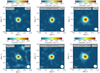 |
Fig. 1 Integrated intensity maps of the 34SO2 111,11−100,10 (Eup = 60.1 K, top) and O13CS 18–17 (Eup = 99.5 K, bottom) lines for 744757A, G318.0489p00.0854B, and G345.5043p00.3480. The integration limits are set to [−2, 2] km s−1 with respect to the sources’ Vlsr. The white star denotes the source positions derived from the peak continuum emission, and the 3σ threshold is denoted by the white line in the color bars. The beam size is shown in the lower-right corner of each panel, and a scale bar is depicted in the lower left. |
2.3 Isotope ratio calibration
Isotopic abundances are dependent on the stellar population and therefore vary as a function of the distance to the Galactic center (DGC). In order to obtain accurate column densities of the main SO2 and OCS isotopologs, it is thus required to calibrate the isotope ratios of (32S/34S), (32S/33S), and (12C/13C) accordingly. Recently, Yan et al. (2023) utilized CS lines in a wide variety of isotopologs observed toward 110 high-mass star-forming regions to derive the equations
![Mathematical equation: $\[\left({ }^{32} \mathrm{S} /{ }^{34} \mathrm{S}\right)=(0.73 \pm 0.36) D_{\mathrm{GC}}+(16.50 \pm 2.07),\]$](/articles/aa/full_html/2024/09/aa50736-24/aa50736-24-eq5.png) (1)
(1)
![Mathematical equation: $\[\left({ }^{32} \mathrm{S} /{ }^{33} \mathrm{S}\right)=(2.64 \pm 0.77) D_{\mathrm{GC}}+(70.80 \pm 5.57),\]$](/articles/aa/full_html/2024/09/aa50736-24/aa50736-24-eq6.png) (2)
(2)
![Mathematical equation: $\[\left({ }^{12} \mathrm{C} /{ }^{13} \mathrm{C}\right)=(4.77 \pm 0.81) D_{\mathrm{GC}}+(20.76 \pm 4.61).\]$](/articles/aa/full_html/2024/09/aa50736-24/aa50736-24-eq7.png) (3)
(3)
The DGC can be calculated based on the source’s distance to Earth (d) and its coordinates. The resulting values for each source are listed in Appendix B and are used to derive 32SO2 and O12CS from the isotopologs. For the solar neighborhood, the ratios are (32S/34S)~22, (32S/33S)~92, and (12C/13C)~59. The uncertainties in the final column densities of 32SO2 and O12CS (henceforth simply SO2 and OCS) are obtained by propagating the errors in the derived column densities of the minor isotopologs together with the uncertainties in Eqs. 1–3 and the typical error of ~0.5 kpc in DGC (see Nazari et al. 2022).
3 Results
3.1 Morphology
The integrated intensity maps of 34SO2 and O13CS for 744757A, G318.0489p00.0854B, and G345.5043p00.3480 are presented in Fig. 1. These are chosen as a representative sample of the sources analyzed in this work. The emission areas of both species are compact (with typical radii of ~1000–3000 au considering all sources) and mostly unresolved, in accordance with the expectation that rare isotopologs likely trace the hot core region with little to no contribution from extended emission. The case of 693050 is an exception in which the 34SO2 and O13CS peaks are offset from the continuum peak (as shown by the white star) by ~4000 au (see Appendix E). This could be the result of optically thick dust at these wavelengths, leading to continuum over-substraction or dust attenuation toward the continuum peak, which has been shown to hide molecular emission in protostellar systems (De Simone et al. 2020). Indeed, the same behavior is observed for CH3OH emission in 693050, in line with this hypothesis (van Gelder et al. 2022b). Higher spatial resolution is required to fully distinguish the species’ emitting regions. Still, some spatial information can be acquired by comparing their best-fit parameters (see Sect. 3.2).
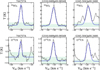 |
Fig. 2 Observed spectra toward 744757A, G318.0489p00.0854B, and G345.5043p00.3480 (gray) superimposed by their best-fit models (blue). The upper panels show the lines of 34SO2 (111,11−100,10), and the lower panels lines of 013CS (18–17). The green shadowed area delimits the 3σ threshold. |
3.2 Fitting results
The best-fit parameters of 34SO2 and O13CS for all sources are listed in Appendix F, together with the corresponding column densities derived for SO2 and OCS. The best-fit models are shown in Fig. 2 for a set of representative sources: 744757A, G318.0489p00.0854B, and G345.5043p00.3480. The models for the remaining sources are presented in Appendix D. 3σ upper limits are provided when line intensities do not surpass this detection threshold. For most sources, the 34SO2 column densities range between 1015 and 1016 cm−2, which corresponds to SO2 column densities of 1016−1017 cm−2. The only exceptions to this trend are the sources for which only N(34SO2) upper limits could be derived.
In comparison, the O13CS column densities are roughly one order of magnitude lower, but given the larger ratios of (12C/13C) compared to (32S/34S), the corresponding N(OCS) values also range between 1016 and 1017 cm−2. Absolute column densities are nevertheless subject to biases such as the assumed emitting area and thus are not ideal to be directly compared. Column density ratios are a more reliable form of comparison to provide information on the chemical inventories of different systems. The column densities derived in this work will be discussed in detail in Sect. 4.
Despite the emissions probed here being largely unresolved, line widths and velocities can be utilized to infer the kinematics of the gas. In Appendix G, we present a comparison between the widths and velocities for both 34SO2 and O13CS with respect to ![Mathematical equation: $\[\mathrm{CH}_3^{18} \mathrm{OH}\]$](/articles/aa/full_html/2024/09/aa50736-24/aa50736-24-eq8.png) . The latter were obtained from the fittings performed by van Gelder et al. (2022a). For some sources, van Gelder et al. (2022a) did not detect
. The latter were obtained from the fittings performed by van Gelder et al. (2022a). For some sources, van Gelder et al. (2022a) did not detect ![Mathematical equation: $\[\mathrm{CH}_3^{18} \mathrm{OH}\]$](/articles/aa/full_html/2024/09/aa50736-24/aa50736-24-eq9.png) , in which cases we compared them to the fitting parameters of the main CH3OH isotopolog (signaled by empty markers). The median offsets of the line widths and peak velocities between the three different species are, respectively, 0.15 and 0.35 km s−1. This is in line with all three molecules tracing a similar compact gas within the hot core region and serves as validation for a comparative analysis of their column density ratios. The fact that no distinctively large discrepancy in FWHM and Vlsr is observed for 34SO2 is an indication that any contribution from outflows to this line can be neglected.
, in which cases we compared them to the fitting parameters of the main CH3OH isotopolog (signaled by empty markers). The median offsets of the line widths and peak velocities between the three different species are, respectively, 0.15 and 0.35 km s−1. This is in line with all three molecules tracing a similar compact gas within the hot core region and serves as validation for a comparative analysis of their column density ratios. The fact that no distinctively large discrepancy in FWHM and Vlsr is observed for 34SO2 is an indication that any contribution from outflows to this line can be neglected.
3.3 Is 34SO2 optically thin?
Line emissions from rare isotopologs are usually assumed to be optically thin. However, this is not necessarily always true, especially for abundant species such as SO2. For this reason, we utilized the four sources in which 33SO2 is detected to assess whether 34SO2 is indeed optically thin. Their best-fit parameters are listed in Appendix H. We derived the column densities of SO2 (i.e., of the main isotopolog) from both N(34SO2) and N(33SO2) separately, using their isotope ratios as described in Sect. 2.3. Figure 3 shows the ratios of SO2 column densities derived from 34SO2 over the 33SO2 counterparts for the four sources. The resulting values are all remarkably close to unity, confirming that both the 34SO2 and 33SO2 lines are indeed optically thin. In fact, the larger the N(SO2)/N(CH3CN) ratios (indicated by the red arrow), the closer the values are to unity. Given that the 33SO2 lines had to be fitted on top of ![Mathematical equation: $\[\mathrm{CH}_3^{13} \mathrm{CN}\]$](/articles/aa/full_html/2024/09/aa50736-24/aa50736-24-eq10.png) (see the discussion in Sect. 2.2), this strongly suggests that the small discrepancies in SO2 column densities calculated from N(33SO2) and N(34SO2) are mostly due to 33SO2 being heavily blended.
(see the discussion in Sect. 2.2), this strongly suggests that the small discrepancies in SO2 column densities calculated from N(33SO2) and N(34SO2) are mostly due to 33SO2 being heavily blended.
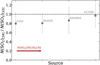 |
Fig. 3 Ratios of N(32SO2) derived from N(34SO2) (numerator) over those derived from N(33SO2) (denominator). The red arrow indicates that the sources are sorted in order of increasing N(SO2)/N(CH3CN) relative abundances. The dashed line highlights the unity mark. G343 stands for source G343.1261-00.0623. |
4 Discussion
As mentioned in Sect. 3.2, column density ratios are a good metric to compare the chemical content of different sources and types of environments. Here we utilized the CH3OH column densities derived by van Gelder et al. (2022a) from minor isotopologs as a basis for comparison. Given the ice origin of methanol, it is possible to deduct information on the chemical history of OCS and SO2 from their relative abundances with respect to ch3oh. In the following subsections, we compare N(OCS)/N(CH3OH) and N(SO2)/N(CH3OH) derived in this work with relative abundances taken from the literature. These encompass gas-phase observations toward both MYSOs and low-mass young stellar objects (LYSOs), ice observations toward protostars and dark clouds, as well as cometary ratios. A complete list of references from which these ratios are taken can be found in Appendix I.
4.1 N(OCS)/N(CH3OH)
Figure 4 shows a comparison of the column density ratios of N(OCS)/N(CH3OH) for various objects. It includes gas-phase observations in low- and high-mass sources as well as ice observations in MYSOs, in dark clouds, and in comets (see Appendix I for a list of references). The ratios derived in this work are shown in blue. In general, no trend in ratio versus luminosity is observed. Indeed, the data points for protostars (including both ice and gas phases) result in a Pearson correlation coefficient (r) of only −0.11. Spearman correlation tests are also performed and yield similar results to Pearson’s for all cases explored in this work. Figure 4 also contain single-dish observations, but since these probe a much larger scale compared to interferometric counterparts, they are not included in the analysis. Furthermore, Kushwahaa et al. (2023) note that their observations could be subject to beam dilution, which could affect the gas-phase ratios for most of the low-mass sources shown in Fig. 4 (with the exception of IRAS 16293–2422 B). Nonetheless, they can still provide information on general trends in abundances. The fairly constant abundance ratios observed throughout all sources indicate that OCS must be formed under similar conditions irrespective of the mass (or luminosity) of the protostar. Considering the drastically different physical conditions experienced by MYSOs and LYSOs during their evolution, particularly regarding their temperatures and UV fields, this lack of correlation with respect to luminosity points to an early formation of the bulk of OCS under cold and dense conditions, prior to the onset of star formation. More data points for low-mass sources would be useful to further constrain any potential trend obscured by the scatter in the ratios.
A considerable number of data points are available for N(OCS)/N(CH3OH) ratios in protostellar ices (Boogert et al. 2022), which enables a statistically significant analysis. Using abundance distribution histograms is an instructive approach to comparing different, large datasets (see, e.g., Öberg et al. 2011). In Fig. 5, the log-transformed N(OCS)/N(CH3OH) ratios are presented for both ice and gas observations toward MYSOs, and are centered on the weighted median of the ALMAGAL dataset (~0.033). Ice lower limits affect the median value by <5% and are thus not included in the analysis. Overall, the ice ratios in MYSOs are slightly lower than the gas-phase counterparts, with a difference of a factor of ~3 between their weighted medians. This discrepancy is remarkably small, and could be due to the uncertainties in the spectral analysis (especially considering the approximation of a fixed Tex). Such strikingly similar ratios provide strong evidence of an icy origin for OCS.
Furthermore, both ice and gas datasets have small scatters, which suggests that the column densities of CH3OH and OCS are subject to similar dependences. A spread factor f, defined by 10 to the power of the weighted 1σ standard deviation measured in log 10 space, serves as a convenient comparison basis between distinct datasets (see, e.g., Nazari et al. 2023). Table 1 summarizes the weighted median gas-phase ratios and spread factors derived in this work for N(OCS)/N(CH3OH), N(SO2)/N(CH3OH), and N(SO2)/N(OCS). For the ALMAGAL subset, the N(OCS)/N(CH3OH) ratios results in f = 2.8, whereas ice observations in MYSOs have f = 1.9. These small scatters suggest similar conditions during the formation of the bulk of OCS and CH3OH, strengthening the conclusion of an icy origin to OCS followed by thermal sublimation. It is worth noting that the lower limits in the available ice ratios are either equivalent to or higher than the corresponding weighted median, so a high abundance tail similar to the gas-phase case could be plausible.
The small scatter for OCS points to an ice environment similar to CH3OH. This agrees with the main proposed chemical routes to form OCS, which involve the sulfurization of CO ices. Laboratory experiments show that OCS ice can be readily formed by the reactions (Ferrante et al. 2008; Jiménez-Escobar et al. 2014; Chen et al. 2015; Nguyen et al. 2021; Santos et al. 2024)
![Mathematical equation: $\[\mathrm{s}{-}\mathrm{CO}+\mathrm{s}{-}\mathrm{S} \rightarrow \mathrm{s}{-}\mathrm{OCS},\]$](/articles/aa/full_html/2024/09/aa50736-24/aa50736-24-eq11.png) (4)
(4)
![Mathematical equation: $\[\mathrm{s}{-}\mathrm{CO}+\mathrm{s}{-}\mathrm{SH} \rightarrow \mathrm{s}{-}\mathrm{HSCO}+\mathrm{s}{-}\mathrm{H} \rightarrow \mathrm{s}{-}\mathrm{OCS}+\mathrm{s}{-}\mathrm{H}_2\]$](/articles/aa/full_html/2024/09/aa50736-24/aa50736-24-eq12.png) (5)
(5)
which can either be induced by thermalized S and SH adsorbed on the ice or as a result of the energetic processing of larger species (e.g., CO2 and H2S). Indeed, Boogert et al. (2022) analyzed a large sample of ice observations toward massive protostars and conclude that OCS and CH3OH column densities are correlated, pointing to an OCS formation concomitant with CH3OH during the dense pre-stellar core stage, with both sharing CO as a common precursor.
Comparisons with dark clouds prior to star formation and comets are also relevant to constrain the evolution of sulfur species in both solid and gas phases. Observed N(OCS)/N(CH3OH) ice ratios in dark clouds agree strikingly well with the protostellar observations toward both ice and gas. This is in full support of the hypothesis that OCS is formed in the ices within pre-stellar cores. Caution should be taken when comparing these values, however, since only two data points are available for ices in pre-stellar cores so far (McClure et al. 2023). Nonetheless, it can still provide the basis for an interesting preliminary comparison. Cometary ratios, in turn, are marginally higher (by a factor of ~4) than the weighted median for ALMAGAL, although their spread encompasses both gas and ice observations. This small discrepancy could be due to additional processing of OCS during the protostellar disk phase (as was also suggested by Boogert et al. 2022) or as a result of selective CH3OH destruction before incorporation into comets. The latter has been previously suggested by Öberg et al. (2011) as one explanation to the depletion of cometary CH3OH, CH4, and CO ices relative to H2O compared to protostars. However, given that OCS and CH3OH are mixed, it seems unlikely that a destruction mechanism could affect one but not the other.
Weighted medians of the column density ratios and spread factors derived in this work for gas-phase species in massive sources (not including upper limits).
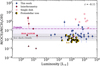 |
Fig. 4 Column density ratios N(OCS)/N(CH3OH) derived in this work (blue markers) for 26 high-mass protostars as a function of luminosity. Literature gas-phase values are shown for comparison (red markers), together with ice values in protostars (yellow and black markers), dark clouds (dashed gray line), and comets (dash-dot purple line). The references can be found in Appendix I. Upper and lower limits toward protostars are denoted by downward and upward facing triangles, respectively. The ranges of values for dark clouds and comets are shown by their respective shadowed areas. For gas-phase ratios, filled markers correspond to interferometric observations, whereas empty markers denote single-dish counterparts. The Pearson correlation coefficient for protostellar ratios in both gas and ices, but excluding single-dish observations and lower limits, is displayed in the upper-right corner. IRAS 16293B stands for the source IRAS 16293-2422 B. |
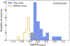 |
Fig. 5 Relative abundance distributions of N(OCS)/N(CH3OH) for the gas-phase observations of massive sources analyzed in this work (blue) compared to ice observations toward 20 MYSOs (Boogert et al. 2022, yellow). Both histograms are normalized to the weighted gas-phase median value derived from the ALMAGAL dataset for 26 high-mass protostars. |
4.2 N(SO2)/N(CH3OH)
Figure 6 shows a comparison of the column density ratios of N(SO2)/N(CH3OH). Similarly to OCS, no correlation is observed for the column density ratios in protostars as a function of luminosity (Pearson r = −0.08), in support of the hypothesis of an early formation during the pre-stellar core stage. One caveat to this conclusion is that the gaseous SO2 column densities in LYSOs are derived from its major isotopolog for most sources (light-red points in Fig. 6), which could contain appreciable contamination from outflow emission and could be optically thick. In fact, Artur de la Villarmois et al. (2023) estimate that ~40% of the SO2 emission in their study is extended. The only exception among low-mass sources is the data point corresponding to IRAS 16293–2422 B, for which SO2 column densities are derived from 34SO2 (dark-red point in Fig. 6). Further works focused on compact, optically thin SO2 emission (as traced by, e.g., 34SO2) in low-mass sources are warranted to further evaluate this hypothesis.
In contrast to OCS, ice ratios of N(SO2)/N(CH3OH) in protostars are still scarce. However, the available values so far for both high-mass and low-mass sources taken from Boogert et al. (1997, 2022) and Rocha et al. (2024) agree fairly well with the median gas-phase ratios derived in this study. The weighted median for our subset of MYSOs (excluding upper limits) is ~0.044, which is consistent with both ice ratios of 0.06±0.04 and 0.07±0.04 in a low- and high-mass source, respectively. This agrees with the hypothesis that SO2 is primarily formed in ices prior to the onset of star formation, and later sublimates upon thermal heating by the protostar.
The scatter in the ALMAGAL values is considerably larger than that for OCS, which suggests that the column densities of CH3OH and SO2 are subject to different dependences. For the ALMAGAL subset, N(SO2)/N(CH3OH) ratios result in f = 5.8. For comparison, oxygen- and nitrogen-bearing complex organic molecules typically have N(X)/N(CH3OH) spread factors of f ≲3.5 (Nazari et al. 2022; Chen et al. 2023). There are likely two reasons behind this large scatter for SO2: one related to both CH3OH and SO2 ice environments, and another related to post-desorption processing of SO2.
Compared to methanol, the body of knowledge on interstellar SO2 formation in cold environments is still somewhat scarce. Currently, its main proposed formation routes generally involve SO and a source of oxygen as reactants (Hartquist et al. 1980; Charnley 1997; Atkinson et al. 2004; Blitz et al. 2000; Woods et al. 2015; Vidal & Wakelam 2018; Laas & Caselli 2019):
![Mathematical equation: $\[\mathrm{SO}+\mathrm{OH} \rightarrow \mathrm{SO}_2+\mathrm{H},\]$](/articles/aa/full_html/2024/09/aa50736-24/aa50736-24-eq13.png) (6)
(6)
![Mathematical equation: $\[\mathrm{SO}+\mathrm{O}_2 \rightarrow \mathrm{SO}_2+\mathrm{O},\]$](/articles/aa/full_html/2024/09/aa50736-24/aa50736-24-eq14.png) (7)
(7)
![Mathematical equation: $\[\mathrm{SO}+\mathrm{O} \rightarrow \mathrm{SO}_2.\]$](/articles/aa/full_html/2024/09/aa50736-24/aa50736-24-eq15.png) (8)
(8)
In the gas phase, such routes are usually not viable at temperatures below 100 K (e.g., van Gelder et al. 2021). One exception might be Reaction 6, for which rate constants have been predicted to range from ~(2–3) × 10−10 cm3 s−1 for temperatures between 10 and 100 K (Fuente et al. 2019). Still, observed gaseous abundances of SO2 in both diffuse and dense clouds are ~10−6−10−5 with respect to CO (Turner 1995; Cernicharo et al. 2011, see also Table 4 in Laas & Caselli 2019), which are three to four orders of magnitude lower than ice abundances. Adsorption of SO2 from the gas phase therefore cannot account for the ice observations. Rather, solid-phase routes to SO2 must be considered, for which Reactions 6–8 are also good candidates (Smardzewski 1978; Moore et al. 2007; Ferrante et al. 2008; Chen et al. 2015; Vidal et al. 2017).
Like SO2, gas-phase abundances of SO with respect to CO are still orders of magnitude smaller than those of SO2 in the ices (Turner 1995; Lique et al. 2006; Neufeld et al. 2015). Thus, even if all SO adsorbed from the gas phase would be converted to SO2, it would still be insufficient to explain SO2 abundances. Alternatively, S atoms adsorbed on the ices could react with O or OH to form SO through
![Mathematical equation: $\[\mathrm{s}{-}\mathrm{S}+\mathrm{s}{-}\mathrm{O} \rightarrow \mathrm{s}{-}\mathrm{SO},\]$](/articles/aa/full_html/2024/09/aa50736-24/aa50736-24-eq16.png) (9)
(9)
![Mathematical equation: $\[\mathrm{s}{-}\mathrm{S}+\mathrm{s}{-}\mathrm{OH} \rightarrow \mathrm{s}{-}\mathrm{SO}+\mathrm{s}{-}\mathrm{H},\]$](/articles/aa/full_html/2024/09/aa50736-24/aa50736-24-eq17.png) (10)
(10)
which in turn can lead to SO2 ice via Reactions 6–8. Atomic S can also directly form SO2 ice by reacting with O2:
![Mathematical equation: $\[\mathrm{s}{-}\mathrm{S}+\mathrm{s}{-}\mathrm{O}_2 \rightarrow \mathrm{s}{-}\mathrm{SO}_2.\]$](/articles/aa/full_html/2024/09/aa50736-24/aa50736-24-eq18.png) (11)
(11)
In addition to the atomic form, interactions of HS radicals with O can efficiently produce SO ice:
![Mathematical equation: $\[\mathrm{s}{-}\mathrm{HS}+\mathrm{s}{-}\mathrm{O} \rightarrow \mathrm{s}{-}\mathrm{SO}+\mathrm{s}{-}\mathrm{H}.\]$](/articles/aa/full_html/2024/09/aa50736-24/aa50736-24-eq19.png) (12)
(12)
Most of these routes have been probed in the laboratory by a number of experimental works involving H2S ices mixed with oxygen-bearing molecules (e.g., CO2 or H2O) and exposed to energetic processing (such as UV photons or protons) to generate the open-shell species (Smardzewski 1978; Moore et al. 2007; Ferrante et al. 2008; Chen et al. 2015). Indeed, HS radicals are thought to be formed in ices via both the hydrogenation of adsorbed S atoms and the destruction of H2S molecules. The latter can occur either through energetic processing, as mentioned above, or due to H-induced abstraction reactions (Oba et al. 2018, 2019; Santos et al. 2023). Furthermore, Laas & Caselli (2019) assert that Reactions 7 and 8 are hindered in ices due to the high diffusion and binding energies of the reactants. Radical and atom formation through energetic processing could partially circumvent this issue.
Irrespective of the mechanism to originate SO2, all routes require an oxygen-rich environment to take place. Such an environment is more likely to occur in the earlier phases of the pre-stellar stage, during which H2O ices grow from the hydrogenation of O, O2, and O3 (e.g., Tielens & Hagen 1982; Miyauchi et al. 2008; Ioppolo et al. 2008; Lamberts et al. 2016). Therefore, SO2 should be formed simultaneously with H2O during the low-density stage of pre-stellar cores. In contrast, CH3OH is mainly formed at a much later stage, when densities are high enough for CO to catastrophically freeze-out onto the grains (Av > 9, nH ≳ 105 cm−3). This discrepancy in the formation timeline of the two species means that they will be subject to different physical conditions and collapse timescales, which may explain the large scatter in the observed ratios. While it is true that ice observations of SO2 have so far been best described by laboratory measurements of SO2 in a CH3OH-rich environment (Boogert et al. 1997; Rocha et al. 2024), the SO2 ice feature at 7.6 μm was shown to be highly sensitive to ice mixtures and temperatures (Boogert et al. 1997). Hence, further systematic infrared characterizations of SO2, perhaps with a combination of tertiary ice mixtures including H2O, would be beneficial to better constrain the chemical environment of this molecule.
A complementary explanation for the scatter in N(SO2)/N(CH3OH) is the reprocessing of SO2 in the gas phase. The SO2 emission probed in this work traces the hot core region surrounding the protostar, where thermal heating has led the volatile ice content to fully sublimate. At the typically warmer temperatures of such environments (≳100 K), the conditions become favorable for Reactions 6–8 to take place in the gas phase (Hartquist et al. 1980; van Gelder et al. 2021). Given the large variation of source structures and physical conditions associated with massive protostars, the degree to which such reactions occur will likely vary considerably from source to source and are thus expected to result in a wide scatter of SO2 column densities. Indeed, the models in Vidal & Wakelam (2018) predict that the gaseous SO2 abundances in protostars are particularly subject to large variations depending on the composition of the parent cloud and the temperature. Furthermore, van Gelder et al. (2021) show that gas-phase SO2 formation is strongly linked to the local UV radiation field since the strength of the latter will largely affect the distribution of reactants. These properties are expected to vary considerably from one massive source to another.
In addition to SO2, CH3OH ices typically show considerable variations in column density from source to source (Öberg et al. 2011), which could be contributing to the scatter seen for N(SO2)/N(CH3OH). Nonetheless, the larger spread for N(SO2) compared to other species relative to N(CH3OH) (e.g., Nazari et al. 2022; Chen et al. 2023 and the N(OCS)/N(CH3OH) ratios in this work) points to a significant effect directly associated with SO2. Differences in the emitting area of SO2 and CH3OH could also play a part in the scatter (Nazari et al. 2024), albeit to a lesser extent since experimental laboratory sublimation temperatures of SO2 and CH3OH are generally quite similar (at ~120 K and ~145 K, respectively; Kaňuchová et al. 2017; Mifsud et al. 2023; Carrascosa et al. 2023). Co-desorption with H2O can potentially raise the sublimation temperature of SO2, but not enough to result in an appreciable difference to CH3OH (see, e.g., Fraser et al. 2001 for sublimation temperatures of H2O). Overall, both the origin of SO2 in ices and its fate after sublimation are likely to play a part in the large scatter seen in Fig. 6.
In dark clouds, the ice ratios of N(SO2)/N(CH3OH) are generally lower than in the protostellar phase (both for ice and gas observations) by about one order of magnitude. This discrepancy could indicate some additional production of SO2 during the protostellar phase, conceivably due to the enhanced UV radiation field produced in such environments. Cometary ratios are marginally higher, but still in a reasonably good agreement with protostellar ices, and are larger than the weighted median for gasphase MYSOs by a factor of ~6. As for the case of OCS, causes for this enhancement could be additional processing of SO2 during the protostellar disk phase, or as a result of selective CH3OH destruction before incorporation into comets. Given that SO2 and CH3OH are proposed to inhabit different ice phases, this supposition is not a priori unreasonable. In summary, the ratios shown in Fig. 6 support the hypothesis of a moderate, but not complete inheritance of SO2 ices from the pre-stellar phase into comets.
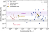 |
Fig. 6 Same as Fig. 4, but for N(SO2)/N(CH3OH). Literature ratios with N(SO2) derived from the main isotopolog are signaled by light red markers to differentiate them from values derived from 34SO2, which are shown in darker red. The data point for the low-mass protostellar ice ratio corresponds to the JWST observations toward IRAS 2A (Rocha et al. 2024), and the high-mass ice ratios correspond to airborne (KAO) and ground-base (IRTF) observations toward NGC 7538 IRS 9 (upper limit) and W33A (Boogert et al. 1997, 2022). |
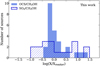 |
Fig. 7 Same as Fig. 5, but for N(SO2)/N(CH3OH) (hatched) and N(OCS)/N(CH3OH) (filled) gas-phase observations from the ALMAGAL dataset. In this case, each ratio is normalized to its own weighted median value. |
4.3 SO2 versus OCS
The column density ratios for SO2/OCS as a function of luminosity agree with the conclusions drawn in the previous subsections (see Appendix J). Figure 7 presents the distribution histograms of N(SO2) and N(OCS) with respect to N(CH3OH) derived in this work. Each N(X)/N(CH3OH) is normalized to its own weighted median, so that both distributions are centered on 1 (i.e., 0 in log space). This figure clearly shows the distinctive behaviors of SO2 and OCS, emphasizing that the latter is likely much more strongly linked to CH3OH than the former. Furthermore, it suggests that the reprocessing of SO2 upon desorption is much more drastic than for OCS, in agreement with the models in Vidal & Wakelam (2018).
Another relevant source of information is to compare the direct correlation between SO2 and OCS abundances with respect to CH3OH (Fig. 8). Based on the derived Pearson coefficient (r = 0.32), a weak correlation appears to exist between N(SO2)/N(CH3OH) and N(OCS)/N(CH3OH). This is supported by the Spearman’s correlation test, which yields a coefficient of ρ = 0.38 with a p-value of 0.05. The fact that this association is weak is unsurprising, since the bulk of SO2 and OCS probably originate from two different ice environments, which means that their chemistry cannot be strongly linked. Nonetheless, some modest connection seems to be present between the two sulfur-bearing species. This could be due, for instance, to one species providing a source of sulfur that is converted into the other. Indeed, SO2 ices can be dissociated into S atoms upon energetic processing, which could in turn react with CO to form OCS. Likewise, OCS molecules can also yield S atoms upon fragmentation, which in turn can react with H2O to form SO2 (Ferrante et al. 2008). Alternatively, this correlation could be the result of a common precursor to both species, such as atomic S or SH radicals. We emphasize, however, that the correlation is weak and reliant on the high-abundance end of the range of values, and thus should be considered with caution.
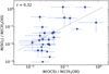 |
Fig. 8 Relative abundances N(SO2)/N(CH3OH) versus N(OCS)/N(CH3OH) for the ALMAGAL dataset analyzed in this work. Upper limits in the N(SO2)/N(CH3OH) ratios are denoted by downward facing triangles. The Pearson correlation coefficient (excluding upper limits) is shown in the upper-left corner, and the dotted line traces the 1:1 relation. |
5 Conclusions
In this work we analyzed the emission of OCS and SO2 toward 26 line-rich MYSOs observed as part of the ALMAGAL survey. We compared their abundances with respect to methanol with other gas-phase observations toward low-mass sources, as well as in interstellar ices and comets. Our main findings are as follows:
The gaseous column density ratios of OCS/CH3OH and SO2/CH3OH show no trend with respect to luminosity, pointing to an early onset formation of both sulfur-bearing molecules before star formation begins. The ratios in protostellar ices are consistent with the weighted medians of the ALMAGAL dataset, suggesting an icy origin for both OCS and SO2 followed by thermal sublimation upon heating from the protostar;
A large scatter in relative abundances is observed with ALMAGAL for gaseous SO2/CH3OH (f = 5.8), but not for OCS/CH3OH (f = 2.8). We suggest that this is due to different chemical environments during the formation of SO2 and OCS, with the former being formed during the low-density phase of cold clouds, and the latter’s formation mostly taking place during the later, high-density pre-stellar stage. OCS and CH3OH both originate from reactions with CO ice. Post-desorption processing likely also contributes to the spread in N(SO2)/N(CH3OH);
For OCS, dark cloud ice values are in remarkably good agreement with both protostellar ice and gas observations. Cometary ratios are also quite similar, at only a factor of ~4 higher. Some extra formation of OCS during the protostellar disk phase has been suggested as a root for this difference, as well as selective destruction of CH3OH. Nonetheless, all ratios point to a significant inheritance of OCS ices throughout the different stages of star formation;
The gaseous abundances of SO2 relative to CH3OH derived in this work agree with both dark-cloud and cometary ice ratios. Values in comets are generally slightly higher (by a factor of ~6) than in protostars, which in turn are higher than in dark clouds. This could indicate some additional formation of SO2 during the protostellar and protoplanetary-disk phases, although selective destruction of CH3OH could also explain such observations in the latter case;
A weak correlation (r = 0.32) is found between N(SO2)/N(CH3OH) and N(OCS)/N(CH3OH). While the bulk of these ices is likely formed in different environments on two distinct evolutionary timescales, some interconversion between SO2 and OCS is possible and could lead to a weak association. This could also result from a common precursor of the two species, arguably S or HS.
Overall, our findings suggest that OCS and SO2 differ significantly in both their formation and destruction pathways, but could still potentially share a common history. It should be noted that the dataset studied here is biased in favor of line-rich sources and therefore our results might not represent all massive protostars. Furthermore, it is clear that more observational constraints on interstellar ice column densities of sulfur-bearing species, and in particular of SO2, are paramount to building a more complete understanding of the origin and fate of sulfur. The JWST offers a unique opportunity for such constraints to be explored in depth.
Acknowledgements
Astrochemistry at Leiden is supported by funding from the European Research Council (ERC) under the European Union’s Horizon 2020 research and innovation programme (grant agreement No. 101019751 MOLDISK) and the Danish National Research Foundation through the Center of Excellence “InterCat” (Grant agreement no.: DNRF150).
Appendix A Example of an excluded source
Figure A.1 contains an example of a source that was excluded from the analysis because of large divergences in the spectral properties between 34SO2 and O13CS, in this case potentially due to self absorption of the 34SO2 lines.
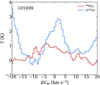 |
Fig. A.1 Superimposed lines of 34SO2 (red) and O13CS (blue) observed toward 101899. |
Appendix B Source properties and observational parameters
The observational parameters for each source and their physical properties are listed in Table B.1.
Observational parameters and physical properties of the sources.
Appendix C List of transitions
Table C lists all the transitions of 34SO2, 33SO2, and O13CS with Eup < 800 K and Aij > 10−6 s−1 covered in the data.
Covered transitions.
Appendix D Best-fit models for all sources
Figures D.1 and D.2 show the best-fit models derived by the grid-fitting approach for each source in the ALMAGAL subset analyzed here. The former contains the results for 34SO2, and the latter for O13CS.
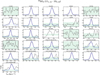 |
Fig. D.1 Observed spectra toward each source (gray) superimposed by its best-fit model for 34SO2 (blue). The green shadowed area delimits the 3σ threshold. The name of each source is shown on the top of each panel. |
Appendix E Integrated intensity map of 693050
Figure E.1 shows the integrated intensity maps of source 693050 for 34SO2 111,11−100,10 and O13CS 18–17. The offset in the emission to the continuum peak is likely due to effects of optically thick dust at these wavelengths.
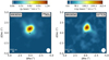 |
Fig. E.1 Integrated intensity maps of the 34SO2 111,11−100,10 (left) and O13CS 18–17 (right) lines for 693050. The integration limits are set to [-5, 5] km s−1 with respect to the source’s Vlsr. The white star denotes the source positions derived from the continuum emission, and the 3σ threshold is delimited by the white line in the color bars. The beam size is shown in the lower-right corner of each panel, and a scale bar is depicted in the lower left. |
Appendix F Best-fit parameters of 34SO2 and O13CS
Tables F.1 and F.2 list the best-fit parameters for 34SO2 and O13CS, respectively, obtained with the grid fitting approach toward all sources. The isotope ratios for each source and corresponding estimated column densities of the main isotopologs are also reported.
Fitting results for 34SO2.
Fitting results for O13CS.
Appendix G FWHM and Vlsr of 34SO2 and O13CS compared to CH3OH
Figure G.1 shows the ratios of FWHM and differences of Vlsr for 34SO2 and O13CS with respect to CH3OH.
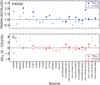 |
Fig. G.1 FWHM ratios (upper panel) and Vlsr differences (lower panel) with respect to |
![Mathematical equation: $\[\mathrm{CH}_3^{18} \mathrm{OH}\]$](/articles/aa/full_html/2024/09/aa50736-24/aa50736-24-eq21.png)
![Mathematical equation: $\[\mathrm{CH}_3^{18} \mathrm{OH}\]$](/articles/aa/full_html/2024/09/aa50736-24/aa50736-24-eq22.png)
Appendix H Best-fit parameters of 33SO2
Table H.1 lists the best-fit parameters for the 33SO2 transitions in the sources where it could be constrained.
Fitted parameters for 33SO2.
Appendix I Literature ratios
Table I.1 lists the literature values for N(SO2)/N(CH3OH), N(OCS)/N(CH3OH), and N(SO2)/N(OCS) gathered in this work.
References of literature ratios.
Appendix J N(SO2)/N(OCS)
The ratios of the derived column densities for SO2 and OCS are shown in Fig. J.1 as a function of luminosity. For comparison, ratios measured in the gas phase of low-mass sources are also shown, together with ice observations toward comets, dark clouds, as well as both low- and high-mass protostars.
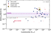 |
Fig. J.1 Same as Fig. 4, but for N(SO2)/N(OCS). Literature ratios with N(SO2) derived from the main isotopolog are signaled by light red markers to differentiate them from values derived from 34SO2, which are shown in darker red. |
References
- Agúndez, M., Marcelino, N., Cernicharo, J., Roueff, E., & Tafalla, M. 2019, A&A, 625, A147 [Google Scholar]
- Altwegg, K., Combi, M., Fuselier, S. A., et al. 2022, MNRAS, 516, 3900 [NASA ADS] [CrossRef] [Google Scholar]
- Anderson, D. E., Bergin, E. A., Maret, S., & Wakelam, V. 2013, ApJ, 779, 141 [Google Scholar]
- Artur de la Villarmois, E., Guzmán, V. V., Yang, Y. L., Zhang, Y., & Sakai, N. 2023, A&A, 678, A124 [NASA ADS] [CrossRef] [EDP Sciences] [Google Scholar]
- Asplund, M., Grevesse, N., Sauval, A. J., & Scott, P. 2009, ARA&A, 47, 481 [NASA ADS] [CrossRef] [Google Scholar]
- Atkinson, R., Baulch, D. L., Cox, R. A., et al. 2004, Atmos. Chem. Phys., 4, 1461 [NASA ADS] [CrossRef] [Google Scholar]
- Bergner, J. B., Öberg, K. I., & Rajappan, M. 2017, ApJ, 845, 29 [Google Scholar]
- Biver, N., Bockelée-Morvan, D., Moreno, R., et al. 2015, Sci. Adv., 1, 1500863 [NASA ADS] [CrossRef] [Google Scholar]
- Biver, N., Bockelée-Morvan, D., Boissier, J., et al. 2021a, A&A, 648, A49 [EDP Sciences] [Google Scholar]
- Biver, N., Bockelée-Morvan, D., Lis, D. C., et al. 2021b, A&A, 651, A25 [NASA ADS] [CrossRef] [EDP Sciences] [Google Scholar]
- Blake, G. A., Sutton, E. Masson, C. R., & Phillips, T. G. 1987, ApJ, 315, 621 [NASA ADS] [CrossRef] [Google Scholar]
- Blake, G. A., van Dishoeck, E. F., Jansen, D. J., Groesbeck, T. D., & Mundy, L. G. 1994, ApJ, 428, 680 [NASA ADS] [CrossRef] [Google Scholar]
- Blitz, M. A., McKee, K. W., & Pilling, M. J. 2000, Proc. Combust. Inst., 28, 2491 [CrossRef] [Google Scholar]
- Bockelée-Morvan, D., Lis, D. C., Wink, J. E., et al. 2000, A&A, 353, 1101 [Google Scholar]
- Boogert, A. C. A., Schutte, W. A., Helmich, F. P., Tielens, A. G. G. M., & Wooden, D. H. 1997, A&A, 317, 929 [NASA ADS] [Google Scholar]
- Boogert, A. C. A., Blake, G. A., & Tielens, A. G. G. M. 2002, ApJ, 577, 271 [NASA ADS] [CrossRef] [Google Scholar]
- Boogert, A. C. A., Brewer, K., Brittain, A., & Emerson, K. S. 2022, ApJ, 941, 32 [NASA ADS] [CrossRef] [Google Scholar]
- Booth, A. S., Temmink, M., van Dishoeck, E. F., et al. 2024, AJ, 167, 165 [NASA ADS] [CrossRef] [Google Scholar]
- Bouscasse, L., Csengeri, T., Belloche, A., et al. 2022, A&A, 662, A32 [NASA ADS] [CrossRef] [EDP Sciences] [Google Scholar]
- Calmonte, U., Altwegg, K., Balsiger, H., et al. 2016, MNRAS, 462, S253 [NASA ADS] [CrossRef] [Google Scholar]
- Carrascosa, H., Satorre, M. Á., Escribano, B., Martín-Doménech, R., & Muñoz Caro, G. M. 2023, MNRAS, 525, 2690 [NASA ADS] [CrossRef] [Google Scholar]
- Cartwright, R. J., Nordheim, T. A., Cruikshank, D. P., et al. 2020, ApJ, 902, L38 [NASA ADS] [CrossRef] [Google Scholar]
- Cernicharo, J., Spielfiedel, A., Balança, C., et al. 2011, A&A, 531, A103 [NASA ADS] [CrossRef] [EDP Sciences] [Google Scholar]
- Cernicharo, J., Marcelino, N., Roueff, E., et al. 2012, ApJ, 759, L43 [NASA ADS] [CrossRef] [Google Scholar]
- Cesaroni, R., Hofner, P., Araya, E., & Kurtz, S. 2010, A&A, 509, A50 [NASA ADS] [CrossRef] [EDP Sciences] [Google Scholar]
- Charnley, S. B. 1997, ApJ, 481, 396 [NASA ADS] [CrossRef] [Google Scholar]
- Charnley, S. B., Tielens, A. G. G. M., & Millar, T. J. 1992, ApJ, 399, L71 [Google Scholar]
- Chen, Y. J., Juang, K. J., Nuevo, M., et al. 2015, ApJ, 798, 80 [Google Scholar]
- Chen, Y., van Gelder, M. L., Nazari, P., et al. 2023, A&A, 678, A137 [NASA ADS] [CrossRef] [EDP Sciences] [Google Scholar]
- Codella, C., Bianchi, E., Podio, L., et al. 2021, A&A, 654, A52 [NASA ADS] [CrossRef] [EDP Sciences] [Google Scholar]
- Cuppen, H. M., van Dishoeck, E. F., Herbst, E., & Tielens, A. G. G. M. 2009, A&A, 508, 275 [NASA ADS] [CrossRef] [EDP Sciences] [Google Scholar]
- Cuppen, H. M., Ioppolo, S., Romanzin, C., & Linnartz, H. 2010, Phys. Chem. Chem. Phys. (Incorp. Faraday Trans.), 12, 12077 [NASA ADS] [CrossRef] [Google Scholar]
- De Simone, M., Ceccarelli, C., Codella, C., et al. 2020, ApJ, 896, L3 [NASA ADS] [CrossRef] [Google Scholar]
- Dello Russo, N., DiSanti, M. A., Mumma, M. J., Magee-Sauer, K., & Rettig, T. W. 1998, Icarus, 135, 377 [NASA ADS] [CrossRef] [Google Scholar]
- Dello Russo, N., Kawakita, H., Vervack, R. J., & Weaver, H. A. 2016, Icarus, 278, 301 [NASA ADS] [CrossRef] [Google Scholar]
- Drdla, K., Knapp, G. R., & van Dishoeck, E. F. 1989, ApJ, 345, 815 [Google Scholar]
- Drozdovskaya, M. N., van Dishoeck, E. F., Jørgensen, J. K., et al. 2018, MNRAS, 476, 4949 [Google Scholar]
- Dulieu, F., Amiaud, L., Congiu, E., et al. 2010, A&A, 512, A30 [NASA ADS] [CrossRef] [EDP Sciences] [Google Scholar]
- Dungee, R., Boogert, A., DeWitt, C. N., et al. 2018, ApJ, 868, L10 [NASA ADS] [CrossRef] [Google Scholar]
- Elia, D., Molinari, S., Schisano, E., et al. 2017, MNRAS, 471, 100 [NASA ADS] [CrossRef] [Google Scholar]
- Elia, D., Merello, M., Molinari, S., et al. 2021, MNRAS, 504, 2742 [NASA ADS] [CrossRef] [Google Scholar]
- Esplugues, G., Fuente, A., Navarro-Almaida, D., et al. 2022, A&A, 662, A52 [NASA ADS] [CrossRef] [EDP Sciences] [Google Scholar]
- Esplugues, G., Rodríguez-Baras, M., San Andrés, D., et al. 2023, A&A, 678, A199 [NASA ADS] [CrossRef] [EDP Sciences] [Google Scholar]
- Ferrante, R. F., Moore, M. H., Spiliotis, M. M., & Hudson, R. L. 2008, ApJ, 684, 1210 [NASA ADS] [CrossRef] [Google Scholar]
- Fontani, F., Roueff, E., Colzi, L., & Caselli, P. 2023, A&A, 680, A58 [NASA ADS] [CrossRef] [EDP Sciences] [Google Scholar]
- Fraser, H. J., Collings, M. P., McCoustra, M. R. S., & Williams, D. A. 2001, MNRAS, 327, 1165 [Google Scholar]
- Fuchs, G. W., Cuppen, H. M., Ioppolo, S., et al. 2009, A&A, 505, 629 [NASA ADS] [CrossRef] [EDP Sciences] [Google Scholar]
- Fuente, A., Cernicharo, J., Agúndez, M., et al. 2010, A&A, 524, A19 [CrossRef] [EDP Sciences] [Google Scholar]
- Fuente, A., Navarro, D. G., Caselli, P., et al. 2019, A&A, 624, A105 [NASA ADS] [CrossRef] [EDP Sciences] [Google Scholar]
- Fuente, A., Treviño-Morales, S. P., Alonso-Albi, T., et al. 2021, MNRAS, 507, 1886 [NASA ADS] [CrossRef] [Google Scholar]
- Fuente, A., Rivière-Marichalar, P., Beitia-Antero, L., et al. 2023, A&A, 670, A114 [NASA ADS] [CrossRef] [EDP Sciences] [Google Scholar]
- Gibb, E., Nummelin, A., Irvine, W. M., Whittet, D. C. B., & Bergman, P. 2000, ApJ, 545, 309 [NASA ADS] [CrossRef] [Google Scholar]
- Gieser, C., Semenov, D., Beuther, H., et al. 2019, A&A, 631, A142 [NASA ADS] [CrossRef] [EDP Sciences] [Google Scholar]
- Hartquist, T. W., Dalgarno, A., & Oppenheimer, M. 1980, ApJ, 236, 182 [NASA ADS] [CrossRef] [Google Scholar]
- Hatchell, J., Thompson, M. A., Millar, T. J., & MacDonald, G. H. 1998, A&A, 338, 713 [Google Scholar]
- Heikkilä, A., Johansson, L. E. B., & Olofsson, H. 1999, A&A, 344, 817 [NASA ADS] [Google Scholar]
- Henkel, C., & Bally, J. 1985, A&A, 150, L25 [NASA ADS] [Google Scholar]
- Herbst, E., & van Dishoeck, E. F. 2009, ARA&A, 47, 427 [NASA ADS] [CrossRef] [Google Scholar]
- Herpin, F., Marseille, M., Wakelam, V., Bontemps, S., & Lis, D. C. 2009, A&A, 504, 853 [NASA ADS] [CrossRef] [EDP Sciences] [Google Scholar]
- Hibbitts, C. A., McCord, T. B., & Hansen, G. B. 2000, J. Geophys. Res., 105, 22541 [NASA ADS] [CrossRef] [Google Scholar]
- Hiraoka, K., Ohashi, N., Kihara, Y., et al. 1994, Chem. Phys. Lett., 229, 408 [Google Scholar]
- Hiraoka, K., Miyagoshi, T., Takayama, T., Yamamoto, K., & Kihara, Y. 1998, ApJ, 498, 710 [CrossRef] [Google Scholar]
- Hodyss, R., Johnson, P. V., Stern, J. V., Goguen, J. D., & Kanik, I. 2009, Icarus, 200, 338 [NASA ADS] [CrossRef] [Google Scholar]
- Hofner, P., Wiesemeyer, H., & Henning, T. 2001, ApJ, 549, 425 [Google Scholar]
- Honma, M., Nagayama, T., & Sakai, N. 2015, PASJ, 67, 70 [NASA ADS] [CrossRef] [Google Scholar]
- Ioppolo, S., Cuppen, H. M., Romanzin, C., van Dishoeck, E. F., & Linnartz, H. 2008, ApJ, 686, 1474 [NASA ADS] [CrossRef] [Google Scholar]
- Ioppolo, S., Cuppen, H. M., Romanzin, C., van Dishoeck, E. F., & Linnartz, H. 2010, Phys. Chem. Chem. Phys. (Incorp. Faraday Trans.), 12, 12065 [NASA ADS] [CrossRef] [Google Scholar]
- Jessup, K. L., Spencer, J., & Yelle, R. 2007, Icarus, 192, 24 [NASA ADS] [CrossRef] [Google Scholar]
- Jiménez-Escobar, A., Muñoz Caro, G. M., & Chen, Y. J. 2014, MNRAS, 443, 343 [Google Scholar]
- Jørgensen, J. K., Müller, H. S. P., Calcutt, H., et al. 2018, A&A, 620, A170 [Google Scholar]
- Kaňuchová, Z., Boduch, P., Domaracka, A., et al. 2017, A&A, 604, A68 [CrossRef] [EDP Sciences] [Google Scholar]
- Keane, J. V., Boonman, A. M. S., Tielens, A. G. G. M., & van Dishoeck, E. F. 2001, A&A, 376, L5 [NASA ADS] [CrossRef] [EDP Sciences] [Google Scholar]
- Kolesniková, L., Tercero, B., Cernicharo, J., et al. 2014, ApJ, 784, L7 [Google Scholar]
- Kushwahaa, T., Drozdovskaya, M. N., Tychoniec, Ł., & Tabone, B. 2023, A&A, 672, A122 [NASA ADS] [CrossRef] [EDP Sciences] [Google Scholar]
- Laas, J. C., & Caselli, P. 2019, A&A, 624, A108 [NASA ADS] [CrossRef] [EDP Sciences] [Google Scholar]
- Lamberts, T., Samanta, P. K., Köhn, A., & Kästner, J. 2016, Phys. Chem. Chem. Phys. (Incorp. Faraday Trans.), 18, 33021 [NASA ADS] [CrossRef] [Google Scholar]
- Lamberts, T., Fedoseev, G., Kästner, J., Ioppolo, S., & Linnartz, H. 2017, A&A, 599, A132 [NASA ADS] [CrossRef] [EDP Sciences] [Google Scholar]
- Le Gal, R., Öberg, K. I., Loomis, R. A., Pegues, J., & Bergner, J. B. 2019, ApJ, 876, 72 [Google Scholar]
- Le Gal, R., Öberg, K. I., Teague, R., et al. 2021, ApJS, 257, 12 [NASA ADS] [CrossRef] [Google Scholar]
- Le Roy, L., Altwegg, K., Balsiger, H., et al. 2015, A&A, 583, A1 [NASA ADS] [CrossRef] [EDP Sciences] [Google Scholar]
- Li, J., Wang, J., Zhu, Q., Zhang, J., & Li, D. 2015, ApJ, 802, 40 [Google Scholar]
- Linke, R. A., Frerking, M. A., & Thaddeus, P. 1979, ApJ, 234, L139 [NASA ADS] [CrossRef] [Google Scholar]
- Lique, F., Cernicharo, J., & Cox, P. 2006, ApJ, 653, 1342 [NASA ADS] [CrossRef] [Google Scholar]
- Lumsden, S. L., Hoare, M. G., Urquhart, J. S., et al. 2013, ApJS, 208, 11 [Google Scholar]
- Majumdar, L., Gratier, P., Vidal, T., et al. 2016, MNRAS, 458, 1859 [NASA ADS] [CrossRef] [Google Scholar]
- Manigand, S., Jørgensen, J. K., Calcutt, H., et al. 2020, A&A, 635, A48 [NASA ADS] [CrossRef] [EDP Sciences] [Google Scholar]
- Martín, S., Mauersberger, R., Martín-Pintado, J., García-Burillo, S., & Henkel, C. 2003, A&A, 411, L465 [NASA ADS] [CrossRef] [EDP Sciences] [Google Scholar]
- Martín, S., Martín-Pintado, J., Mauersberger, R., Henkel, C., & García-Burillo, S. 2005, ApJ, 620, 210 [CrossRef] [Google Scholar]
- Mauersberger, R., Henkel, C., & Chin, Y. N. 1995, A&A, 294, 23 [NASA ADS] [Google Scholar]
- McClure, M. K., Rocha, W. R. M., Pontoppidan, K. M., et al. 2023, Nat. Astron., 7, 431 [NASA ADS] [CrossRef] [Google Scholar]
- McGuire, B. A. 2022, ApJS, 259, 30 [NASA ADS] [CrossRef] [Google Scholar]
- McMullin, J. P., Waters, B., Schiebel, D., Young, W., & Golap, K. 2007, in Astronomical Data Analysis Software and Systems XVI, eds. R. A. Shaw, F. Hill, & D. J. Bell (San Francisco: ASP), ASP Conf. Ser., 376, 127 [Google Scholar]
- Mège, P., Russeil, D., Zavagno, A., et al. 2021, A&A, 646, A74 [NASA ADS] [CrossRef] [EDP Sciences] [Google Scholar]
- Mifsud, D. V., Herczku, P., Rahul, K. K., et al. 2023, Phys. Chem. Chem. Phys. (Incorp. Faraday Trans.), 25, 26278 [NASA ADS] [CrossRef] [Google Scholar]
- Mininni, C., Fontani, F., Sánchez-Monge, A., et al. 2021, A&A, 653, A87 [NASA ADS] [CrossRef] [EDP Sciences] [Google Scholar]
- Miyauchi, N., Hidaka, H., Chigai, T., et al. 2008, Chem. Phys. Lett., 456, 27 [CrossRef] [Google Scholar]
- Mokrane, H., Chaabouni, H., Accolla, M., et al. 2009, ApJ, 705, L195 [Google Scholar]
- Molinari, S., Swinyard, B., Bally, J., et al. 2010, A&A, 518, A100 [Google Scholar]
- Moore, M. H., Hudson, R. L., & Carlson, R. W. 2007, Icarus, 189, 409 [CrossRef] [Google Scholar]
- Moullet, A., Lellouch, E., Moreno, R., Gurwell, M. A., & Moore, C. 2008, A&A, 482, 279 [NASA ADS] [CrossRef] [EDP Sciences] [Google Scholar]
- Moullet, A., Lellouch, E., Moreno, R., et al. 2013, ApJ, 776, 32 [NASA ADS] [CrossRef] [Google Scholar]
- Müller, H. S. P., Thorwirth, S., Roth, D. A., & Winnewisser, G. 2001, A&A, 370, L49 [Google Scholar]
- Müller, H. S. P., Schlöder, F., Stutzki, J., & Winnewisser, G. 2005, J. Mol. Struct., 742, 215 [Google Scholar]
- Müller, H. S. P., Belloche, A., Xu, L.-H., et al. 2016, A&A, 587, A92 [NASA ADS] [CrossRef] [EDP Sciences] [Google Scholar]
- Mumma, M. J., Bonev, B. P., Villanueva, G. L., et al. 2011, ApJ, 734, L7 [Google Scholar]
- Navarro-Almaida, D., Le Gal, R., Fuente, A., et al. 2020, A&A, 637, A39 [NASA ADS] [CrossRef] [EDP Sciences] [Google Scholar]
- Nazari, P., van Gelder, M. L., van Dishoeck, E. F., et al. 2021, A&A, 650, A150 [EDP Sciences] [Google Scholar]
- Nazari, P., Meijerhof, J. D., van Gelder, M. L., et al. 2022, A&A, 668, A109 [NASA ADS] [CrossRef] [EDP Sciences] [Google Scholar]
- Nazari, P., Tabone, B., van’t Hoff, M. L. R., Jørgensen, J. K., & van Dishoeck, E. F. 2023, ApJ, 951, L38 [NASA ADS] [CrossRef] [Google Scholar]
- Nazari, P., Tabone, B., Rosotti, G. P., & van Dishoeck, E. F. 2024, Correlations among complex organic molecules around protostars: Effects of physical structure [Google Scholar]
- Neufeld, D. A., Godard, B., Gerin, M., et al. 2015, A&A, 577, A49 [NASA ADS] [CrossRef] [EDP Sciences] [Google Scholar]
- Nguyen, T., Oba, Y., Sameera, W. M. C., Kouchi, A., & Watanabe, N. 2021, ApJ, 922, 146 [NASA ADS] [CrossRef] [Google Scholar]
- Nickerson, S., Rangwala, N., Colgan, S. W. J., et al. 2023, ApJ, 945, 26 [NASA ADS] [CrossRef] [Google Scholar]
- Oba, Y., Tomaru, T., Lamberts, T., Kouchi, A., & Watanabe, N. 2018, Nat. Astron., 2, 228 [NASA ADS] [CrossRef] [Google Scholar]
- Oba, Y., Tomaru, T., Kouchi, A., & Watanabe, N. 2019, ApJ, 874, 124 [NASA ADS] [CrossRef] [Google Scholar]
- Öberg, K. I., Boogert, A. C. A., Pontoppidan, K. M., et al. 2008, ApJ, 678, 1032 [Google Scholar]
- Öberg, K. I., van Dishoeck, E. F., Linnartz, H., & Andersson, S. 2010, ApJ, 718, 832 [Google Scholar]
- Öberg, K. I., Boogert, A. C. A., Pontoppidan, K. M., et al. 2011, ApJ, 740, 109 [Google Scholar]
- Osorio, M., Anglada, G., Lizano, S., & D’Alessio, P. 2009, ApJ, 694, 29 [Google Scholar]
- Oya, Y., Sakai, N., López-Sepulcre, A., et al. 2016, ApJ, 824, 88 [Google Scholar]
- Oya, Y., López-Sepulcre, A., Sakai, N., et al. 2019, ApJ, 881, 112 [Google Scholar]
- Palumbo, M. E., Tielens, A. G. G. M., & Tokunaga, A. T. 1995, ApJ, 449, 674 [NASA ADS] [CrossRef] [Google Scholar]
- Palumbo, M. E., Geballe, T. R., & Tielens, A. G. G. M. 1997, ApJ, 479, 839 [NASA ADS] [CrossRef] [Google Scholar]
- Petuchowski, S. J., & Bennett, C. L. 1992, ApJ, 391, 137 [NASA ADS] [CrossRef] [Google Scholar]
- Phuong, N. T., Chapillon, E., Majumdar, L., et al. 2018, A&A, 616, A5 [NASA ADS] [CrossRef] [EDP Sciences] [Google Scholar]
- Pillai, T., Kauffmann, J., Wyrowski, F., et al. 2011, A&A, 530, A118 [CrossRef] [EDP Sciences] [Google Scholar]
- Pineau des Forêts, G., Roueff, E., Schilke, P., & Flower, D. R. 1993, MNRAS, 262, 915 [CrossRef] [Google Scholar]
- Pontoppidan, K. M. 2006, A&A, 453, L47 [NASA ADS] [CrossRef] [EDP Sciences] [Google Scholar]
- Pontoppidan, K. M., Fraser, H. J., Dartois, E., et al. 2003, A&A, 408, 981 [NASA ADS] [CrossRef] [EDP Sciences] [Google Scholar]
- Qasim, D., Chuang, K. J., Fedoseev, G., et al. 2018, A&A, 612, A83 [NASA ADS] [CrossRef] [EDP Sciences] [Google Scholar]
- Rivière-Marichalar, P., Fuente, A., Goicoechea, J. R., et al. 2019, A&A, 628, A16 [Google Scholar]
- Rivière-Marichalar, P., Fuente, A., Le Gal, R., et al. 2020, A&A, 642, A32 [EDP Sciences] [Google Scholar]
- Rivière-Marichalar, P., Fuente, A., Le Gal, R., et al. 2021, A&A, 652, A46 [NASA ADS] [CrossRef] [EDP Sciences] [Google Scholar]
- Rocha, W. R. M., van Dishoeck, E. F., Ressler, M. E., et al. 2024, A&A, 683, A124 [NASA ADS] [CrossRef] [EDP Sciences] [Google Scholar]
- Rodríguez-Almeida, L. F., Jiménez-Serra, I., Rivilla, V. M., et al. 2021, ApJ, 912, L11 [Google Scholar]
- Romanzin, C., Ioppolo, S., Cuppen, H. M., van Dishoeck, E. F., & Linnartz, H. 2011, J. Chem. Phys., 134, 084504 [NASA ADS] [CrossRef] [Google Scholar]
- Sahu, D., Liu, S.-Y., Su, Y.-N., et al. 2019, ApJ, 872, 196 [Google Scholar]
- Sakai, N., Sakai, T., Hirota, T., et al. 2014, Nature, 507, 78 [Google Scholar]
- Saki, M., Gibb, E. L., Bonev, B. P., et al. 2020, AJ, 160, 184 [Google Scholar]
- Santos, J. C., Chuang, K.-J., Lamberts, T., et al. 2022, ApJ, 931, L33 [NASA ADS] [CrossRef] [Google Scholar]
- Santos, J. C., Linnartz, H., & Chuang, K. J. 2023, A&A, 678, A112 [NASA ADS] [CrossRef] [EDP Sciences] [Google Scholar]
- Santos, J., Linnartz, H., & Chuang, K.-J. 2024, A&A, in press, https://doi.org/10.1051/0004-6361/202451368 [Google Scholar]
- Schuhmann, M., Altwegg, K., Balsiger, H., et al. 2019, ACS Earth Space Chem., 3, 1854 [NASA ADS] [CrossRef] [Google Scholar]
- Semenov, D., Favre, C., Fedele, D., et al. 2018, A&A, 617, A28 [NASA ADS] [CrossRef] [EDP Sciences] [Google Scholar]
- Smardzewski, R. R. 1978, J. Chem. Phys., 68, 2878 [Google Scholar]
- Smith, A. M., Stecher, T. P., & Casswell, L. 1980, ApJ, 242, 402 [NASA ADS] [CrossRef] [Google Scholar]
- Spezzano, S., Sipilä, O., Caselli, P., et al. 2022, A&A, 661, A111 [NASA ADS] [CrossRef] [EDP Sciences] [Google Scholar]
- Tabone, B., Cabrit, S., Bianchi, E., et al. 2017, A&A, 607, L6 [NASA ADS] [CrossRef] [EDP Sciences] [Google Scholar]
- Tafalla, M., Myers, P. C., Mardones, D., & Bachiller, R. 2000, A&A, 359, 967 [NASA ADS] [Google Scholar]
- Taquet, V., Codella, C., De Simone, M., et al. 2020, A&A, 637, A63 [NASA ADS] [CrossRef] [EDP Sciences] [Google Scholar]
- Tieftrunk, A., Pineau des Forets, G., Schilke, P., & Walmsley, C. M. 1994, A&A, 289, 579 [Google Scholar]
- Tielens, A. G. G. M., & Hagen, W. 1982, A&A, 114, 245 [Google Scholar]
- Tielens, A. G. G. M., Tokunaga, A. T., Geballe, T. R., & Baas, F. 1991, ApJ, 381, 181 [NASA ADS] [CrossRef] [Google Scholar]
- Tobin, J. J., Looney, L. W., Li, Z.-Y., et al. 2016, ApJ, 818, 73 [CrossRef] [Google Scholar]
- Turner, B. E. 1995, ApJ, 455, 556 [NASA ADS] [CrossRef] [Google Scholar]
- Tychoniec, Ł., van Dishoeck, E. F., van’t Hoff, M. L. R., et al. 2021, A&A, 655, A65 [NASA ADS] [CrossRef] [EDP Sciences] [Google Scholar]
- van der Tak, F. F. S., van Dishoeck, E. F., & Caselli, P. 2000, A&A, 361, 327 [NASA ADS] [Google Scholar]
- van der Tak, F. F. S., Boonman, A. M. S., Braakman, R., & van Dishoeck, E. F. 2003, A&A, 412, 133 [NASA ADS] [CrossRef] [EDP Sciences] [Google Scholar]
- van der Tak, F. F. S., Chavarría, L., Herpin, F., et al. 2013, A&A, 554, A83 [NASA ADS] [CrossRef] [EDP Sciences] [Google Scholar]
- van Gelder, M. L., Tabone, B., Tychoniec, Ł., et al. 2020, A&A, 639, A87 [NASA ADS] [CrossRef] [EDP Sciences] [Google Scholar]
- van Gelder, M. L., Tabone, B., van Dishoeck, E. F., & Godard, B. 2021, A&A, 653, A159 [CrossRef] [EDP Sciences] [Google Scholar]
- van Gelder, M. L., Jaspers, J., Nazari, P., et al. 2022a, A&A, 667, A136 [NASA ADS] [CrossRef] [EDP Sciences] [Google Scholar]
- van Gelder, M. L., Nazari, P., Tabone, B., et al. 2022b, A&A, 662, A67 [NASA ADS] [CrossRef] [EDP Sciences] [Google Scholar]
- van Gelder, M. L., Ressler, M. E., van Dishoeck, E. F., et al. 2024, A&A, 682, A78 [NASA ADS] [CrossRef] [EDP Sciences] [Google Scholar]
- Vastel, C., Bottinelli, S., Caux, E., Glorian, J. M., & Boiziot, M. 2015, in SF2A-2015: Proceedings of the Annual meeting of the French Society of Astronomy and Astrophysics, 313 [Google Scholar]
- Vastel, C., Quénard, D., Le Gal, R., et al. 2018, MNRAS, 478, 5514 [Google Scholar]
- Vidal, T. H. G., & Wakelam, V. 2018, MNRAS, 474, 5575 [Google Scholar]
- Vidal, T. H. G., Loison, J.-C., Jaziri, A. Y., et al. 2017, MNRAS, 469, 435 [Google Scholar]
- Wada, A., Mochizuki, N., & Hiraoka, K. 2006, ApJ, 644, 300 [Google Scholar]
- Wakelam, V., Castets, A., Ceccarelli, C., et al. 2004, A&A, 413, 609 [NASA ADS] [CrossRef] [EDP Sciences] [Google Scholar]
- Watanabe, N., & Kouchi, A. 2002, ApJ, 571, L173 [Google Scholar]
- Woods, P. M., Occhiogrosso, A., Viti, S., et al. 2015, MNRAS, 450, 1256 [Google Scholar]
- Yan, Y. T., Henkel, C., Kobayashi, C., et al. 2023, A&A, 670, A98 [NASA ADS] [CrossRef] [EDP Sciences] [Google Scholar]
- Yang, Y.-L., Evans, Neal J., I., Smith, A., et al. 2020, ApJ, 891, 61 [CrossRef] [Google Scholar]
- Yang, Y.-L., Sakai, N., Zhang, Y., et al. 2021, ApJ, 910, 20 [Google Scholar]
- Yang, Y.-L., Green, J. D., Pontoppidan, K. M., et al. 2022, ApJ, 941, L13 [NASA ADS] [CrossRef] [Google Scholar]
- Zapata, L. A., Palau, A., Galván-Madrid, R., et al. 2015, MNRAS, 447, 1826 [NASA ADS] [CrossRef] [Google Scholar]
- Zasowski, G., Kemper, F., Watson, D. M., et al. 2009, ApJ, 694, 459 [CrossRef] [Google Scholar]
All Tables
Weighted medians of the column density ratios and spread factors derived in this work for gas-phase species in massive sources (not including upper limits).
All Figures
|
Fig. 1 Integrated intensity maps of the 34SO2 111,11−100,10 (Eup = 60.1 K, top) and O13CS 18–17 (Eup = 99.5 K, bottom) lines for 744757A, G318.0489p00.0854B, and G345.5043p00.3480. The integration limits are set to [−2, 2] km s−1 with respect to the sources’ Vlsr. The white star denotes the source positions derived from the peak continuum emission, and the 3σ threshold is denoted by the white line in the color bars. The beam size is shown in the lower-right corner of each panel, and a scale bar is depicted in the lower left. |
| In the text | |
|
Fig. 2 Observed spectra toward 744757A, G318.0489p00.0854B, and G345.5043p00.3480 (gray) superimposed by their best-fit models (blue). The upper panels show the lines of 34SO2 (111,11−100,10), and the lower panels lines of 013CS (18–17). The green shadowed area delimits the 3σ threshold. |
| In the text | |
|
Fig. 3 Ratios of N(32SO2) derived from N(34SO2) (numerator) over those derived from N(33SO2) (denominator). The red arrow indicates that the sources are sorted in order of increasing N(SO2)/N(CH3CN) relative abundances. The dashed line highlights the unity mark. G343 stands for source G343.1261-00.0623. |
| In the text | |
|
Fig. 4 Column density ratios N(OCS)/N(CH3OH) derived in this work (blue markers) for 26 high-mass protostars as a function of luminosity. Literature gas-phase values are shown for comparison (red markers), together with ice values in protostars (yellow and black markers), dark clouds (dashed gray line), and comets (dash-dot purple line). The references can be found in Appendix I. Upper and lower limits toward protostars are denoted by downward and upward facing triangles, respectively. The ranges of values for dark clouds and comets are shown by their respective shadowed areas. For gas-phase ratios, filled markers correspond to interferometric observations, whereas empty markers denote single-dish counterparts. The Pearson correlation coefficient for protostellar ratios in both gas and ices, but excluding single-dish observations and lower limits, is displayed in the upper-right corner. IRAS 16293B stands for the source IRAS 16293-2422 B. |
| In the text | |
|
Fig. 5 Relative abundance distributions of N(OCS)/N(CH3OH) for the gas-phase observations of massive sources analyzed in this work (blue) compared to ice observations toward 20 MYSOs (Boogert et al. 2022, yellow). Both histograms are normalized to the weighted gas-phase median value derived from the ALMAGAL dataset for 26 high-mass protostars. |
| In the text | |
|
Fig. 6 Same as Fig. 4, but for N(SO2)/N(CH3OH). Literature ratios with N(SO2) derived from the main isotopolog are signaled by light red markers to differentiate them from values derived from 34SO2, which are shown in darker red. The data point for the low-mass protostellar ice ratio corresponds to the JWST observations toward IRAS 2A (Rocha et al. 2024), and the high-mass ice ratios correspond to airborne (KAO) and ground-base (IRTF) observations toward NGC 7538 IRS 9 (upper limit) and W33A (Boogert et al. 1997, 2022). |
| In the text | |
|
Fig. 7 Same as Fig. 5, but for N(SO2)/N(CH3OH) (hatched) and N(OCS)/N(CH3OH) (filled) gas-phase observations from the ALMAGAL dataset. In this case, each ratio is normalized to its own weighted median value. |
| In the text | |
|
Fig. 8 Relative abundances N(SO2)/N(CH3OH) versus N(OCS)/N(CH3OH) for the ALMAGAL dataset analyzed in this work. Upper limits in the N(SO2)/N(CH3OH) ratios are denoted by downward facing triangles. The Pearson correlation coefficient (excluding upper limits) is shown in the upper-left corner, and the dotted line traces the 1:1 relation. |
| In the text | |
|
Fig. A.1 Superimposed lines of 34SO2 (red) and O13CS (blue) observed toward 101899. |
| In the text | |
|
Fig. D.1 Observed spectra toward each source (gray) superimposed by its best-fit model for 34SO2 (blue). The green shadowed area delimits the 3σ threshold. The name of each source is shown on the top of each panel. |
| In the text | |
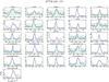 |
Fig. D.2 Same as Fig. D.1, but for O13CS. |
| In the text | |
|
Fig. E.1 Integrated intensity maps of the 34SO2 111,11−100,10 (left) and O13CS 18–17 (right) lines for 693050. The integration limits are set to [-5, 5] km s−1 with respect to the source’s Vlsr. The white star denotes the source positions derived from the continuum emission, and the 3σ threshold is delimited by the white line in the color bars. The beam size is shown in the lower-right corner of each panel, and a scale bar is depicted in the lower left. |
| In the text | |
|
Fig. G.1 FWHM ratios (upper panel) and Vlsr differences (lower panel) with respect to |
| In the text | |
|
Fig. J.1 Same as Fig. 4, but for N(SO2)/N(OCS). Literature ratios with N(SO2) derived from the main isotopolog are signaled by light red markers to differentiate them from values derived from 34SO2, which are shown in darker red. |
| In the text | |
Current usage metrics show cumulative count of Article Views (full-text article views including HTML views, PDF and ePub downloads, according to the available data) and Abstracts Views on Vision4Press platform.
Data correspond to usage on the plateform after 2015. The current usage metrics is available 48-96 hours after online publication and is updated daily on week days.
Initial download of the metrics may take a while.