| Issue |
A&A
Volume 689, September 2024
|
|
|---|---|---|
| Article Number | A98 | |
| Number of page(s) | 16 | |
| Section | The Sun and the Heliosphere | |
| DOI | https://doi.org/10.1051/0004-6361/202450430 | |
| Published online | 05 September 2024 | |
Multi-spacecraft study with the Icarus model
Modelling the propagation of CMEs to Mercury and Earth
1
Department of Mathematics/Centre for mathematical Plasma Astrophysics, KU Leuven, 3001 Leuven, Belgium
2
Institute of Atmospheric Physics CAS, Dept of Space Physics, 14100 Prague, Czech Republic
3
LESIA, Observatoire de Paris, Université PSL, CNRS, Sorbonne Université, Univ. Paris Diderot, Sorbonne Paris Cité, 5 place Jules Janssen, 92195 Meudon, France
4
SUPA, School of Physics and Astronomy, University of Glasgow, G12 8QQ, Glasgow, UK
5
Institute of Physics, University of Maria Curie-Skłodowska, 20 031 Lublin, Poland
Received:
18
April
2024
Accepted:
19
May
2024
Context. Coronal mass ejections (CMEs) are the main drivers of the disturbances in interplanetary space. Earth-directed CMEs can be dangerous, and understanding the CME interior magnetic structure is crucial for advancing space weather studies. It is important to assess the capabilities of a numerical heliospheric model, as a firm understanding of the nature and extent of its limitations can be used to improve the model and the space weather predictions based on it.
Aims. The aim of the present study is to test the capabilities of the recently developed heliospheric model Icarus and the linear force-free spheromak model that has been implemented in it.
Methods. To validate the Icarus space weather modelling tool, two CME events were selected that were observed by two spacecraft located near Mercury and Earth, respectively. This enables us to test the heliospheric model computed with Icarus at two distant locations. The source regions for the CMEs were identified, and the CME parameters were determined and later optimised. Different adaptive mesh refinement levels were applied in the simulations to assess its performance by comparing the simulation results to in situ measurements.
Results. The first CME event erupted at 15:25 on July 9, 2013. The modelled time series were in good agreement with the observations both at MESSENGER and ACE. The second CME event started at 10:25 on February 16, 2014, and was more complicated, as three CME interactions occurred in this event. It was impossible to recover the observed profiles without modelling the other two CMEs that were observed, one before the main CME and one afterward. The parameters for the three CMEs were identified and the three CMEs were modelled in Icarus. For both CME studies, AMR level 3 was sufficient to reconstruct small-scale features near Mercury, while at Earth, AMR level 4 was necessary due to the radially stretched grid that was used.
Conclusions. The profiles obtained at both spacecraft resemble the in situ measurements well. The current limitations of the space weather modelling tool result in an excessively small deceleration of the CME propagation during the CME–CME interaction as measured by MESSENGER and ACE.
Key words: magnetohydrodynamics (MHD) / methods: numerical / methods: observational / Sun: coronal mass ejections (CMEs) / Sun: heliosphere / solar wind
© The Authors 2024
 Open Access article, published by EDP Sciences, under the terms of the Creative Commons Attribution License (https://creativecommons.org/licenses/by/4.0), which permits unrestricted use, distribution, and reproduction in any medium, provided the original work is properly cited.
This article is published in open access under the Subscribe to Open model. Subscribe to A&A to support open access publication.
1. Introduction
Coronal mass ejections (CMEs) are massive eruptive events originating in the solar corona and travelling out into the heliosphere. They are considered the main drivers of space weather disturbances (Gopalswamy et al. 2017). Space weather is the branch of physics that focuses on studying and predicting the physical conditions in the heliosphere, with a particular focus on Earth. Thus, studying the main sources of the disturbances is crucial for advancing space weather studies. CMEs are often associated with solar flares, which are energy bursts within the solar corona. During a CME eruption, a large plasma cloud (up to 1016 g) is expelled from the Sun (Webb & Howard 2012). The speeds of these clouds range between 100 and 3000 km s−1 according to SOHO/LASCO observations. The average speed of a CME was estimated by Webb et al. (2006) to be ∼450 km s−1. CME eruptions occur more frequently during periods of high solar activity. During solar minimum, the number of eruptions decreases and the interplanetary medium is less disturbed.
As a CME travels through space, it interacts with the solar wind. During periods when the Sun is most active, multiple CMEs can be released from nearby regions. When these CMEs come into contact with each other along their propagation in the heliosphere, they create intricate CME–CME interaction regions that travel through the solar wind. CMEs expand as they travel from the Sun, and can reach sizes of ∼10 − 20 R⊙ at as little as 0.1 au from the Sun. The exact eruption scenarios and the interior description of the CMEs are still under debate among solar physicists. Still, it is commonly agreed that the violent eruptions are connected with the release of magnetic energy. The CME interior is not homogeneous and is often associated with complex magnetic flux ropes (Webb & Howard 2012; Cane & Richardson 2003; Vourlidas et al. 2013).
The CMEs can be observed with coronagraphs such as the SOHO/LASCO-C2 and C3 coronagraphs (Brueckner et al. 1995), and the coronagraphs mounted on the two satellites of the Solar Terrestrial Relations Observatory (STEREO, Kaiser 2005)). Interplanetary CMEs (ICMEs) can also be identified from in situ measurements. These ejections have significant features allowing them to be distinguished from solar wind features (Burlaga 1991; Zhang et al. 2021).
There are several limitations to the observation capabilities today. The coronagraph images are useful in estimating or calculating the early evolution characteristics of CMEs. They can provide information about the eruption time, direction, size (spread angle), and speed of the CME. However, these images do not help determine the ejected material’s magnetic field configuration or strength. On the other hand, in situ measurements provide local data on plasma and magnetic field quantities at a specific spacecraft location and time. Therefore, they represent only a trajectory through the enormous magnetic clouds as they pass by the spacecraft, which limits its sampling significantly, as the interior is not homogeneous and is evolving. Therefore, modelling the global evolution of a magnetic cloud is a challenge for the solar physics community.
One way to decrease the uncertainty and increase the number of sampling points is to consider multi-point observations (Burlaga et al. 1982). Numerous new multi-point missions are being proposed and designed, providing greater insight into future events. Multiple spacecraft can help identify historical events when the same CMEs are observed through their alignment at different locations. This approach has enabled scientists to study the interior of CMEs in greater detail, providing a better sampling of these historical events. Often, the knowledge extracted from these multi-point observations is the motivation for proposing such missions to advance our understanding of these events. Today, it is rare for such ‘fortunate’ alignments to occur, which limits the events that can be investigated through this method. However, several studies describe such events observed by multiple spacecraft (Winslow et al. 2015; Grison et al. 2018; Davies et al. 2020; Palmerio et al. 2021; Salman et al. 2020).
CMEs are a global threat to the operation of satellites and ground-based technology on Earth. The CME magnetic field interacts with Earth’s magnetosphere, causing geomagnetic storms that can lead to telecommunication failures and power grid blackouts (Kilpua et al. 2017). Nowadays, with the increased amount of spacecraft and satellites in space, the focus of space weather is not just on Earth but is now spread over the entire heliosphere, as multiple points are being sampled simultaneously. Violent events have shortened the operational lifespan of satellites; for example, the geophysical satellite GOES suffered a shortening of its operational lifespan by three years. Space weather events can cause malfunction of transmission systems. For example, the PRARE instrument on the European Space Agency’s ERS-1 satellite was affected by space weather to the extent that its position can no longer be determined. This makes the interpretation of the measurements of the instrument rather challenging.
The damage caused by regular events, especially during phases of maximum activity of the Sun (explained in the following section), has been estimated to accumulate to an economic loss of 10 billion euros per year (National Research Council 2008). The potential loss from future strong Earth-directed events is increasing continuously because our dependence on telecommunications, navigation, and electronic systems is increasing day to day. In 2019, the National Threat and Hazard Identification and Risk Assessment (THIRA) of the US Federal Emergency Management Agency (FEMA) identified space weather as one of the two threats that could potentially disturb our society globally, the other one being a pandemic (THIRA 2019). Therefore, an unexpected major solar event can cause damage locally on Earth but also interfere with ongoing space missions.
Potential damage can be mitigated if the eruption and its propagation are predicted well in advance, allowing preventive measures. Space weather forecasting has become the standard approach for monitoring the environment surrounding Earth and predicting the arrival time and strength of CMEs.
A new heliospheric modelling tool, Icarus (Verbeke et al. 2022; Baratashvili et al. 2022b), was recently developed at the Centre for Mathematical Plasma-Astrophysics (CmPA, KU Leuven) within the European Heliospheric FORecasting Information Asset project (EUHFORIA, Pomoell & Poedts 2018) as an alternative heliospheric wind and CME evolution model. Icarus is implemented in the MPI-AMRVAC framework (Xia et al. 2018) and performs solar wind and CME simulations with advanced techniques, such as grid stretching and adaptive mesh refinement (AMR), to obtain fast predictions at Earth (Baratashvili et al. 2022b). A magnetised CME model was integrated into Icarus, which allows the modelling of the CME interior magnetic field and investigation of its evolution as the CME travels from the Sun towards the Earth (Baratashvili & Poedts 2024).
To validate the new heliospheric model Icarus and the implemented magnetised spheromak CME model, two CMEs were chosen that were observed by multiple spacecraft from the catalogue presented in Winslow et al. (2015). The first CME case studied here occurred on July 9, 2013, and was observed by the MErcury Surface, Space ENvironment, GEochemistry, and Ranging (MESSENGER) spacecraft near Mercury and the Advanced Composition Explorer (ACE) satellite near Earth. The second event occurred on February 16, 2014, and was observed by MESSENGER and ACE. However, in the latter case, the three-CME interaction was identified near Earth, while at MESSENGER these CMEs do not interact. We model both CME events with Icarus, and compare the time series at MESSENGER and ACE with the observational data. We applied different AMR levels to estimate the performance of Icarus with MESSENGER and ACE data, considering the large radial separation.
The paper is organised as follows: Section 2 presents the numerical setup in Icarus as well as the available CME models and advanced techniques for efficient simulations, such as grid stretching and solution AMR. Section 3 presents the identification of the source, the obtained parameters for modelling the CMEs, and the modelled data at MESSENGER and ACE for the first CME event of July 9, 2013. The analysis of the second CME event of February 16, 2014, is presented in Section 4. The conclusions and outlooks following this study are presented in Section 5.
2. Numerical setup in Icarus
Icarus (Verbeke et al. 2022) is a heliospheric modelling tool implemented in the framework of MPI-AMRVAC (Xia et al. 2018). MPI-AMRVAC, a numerical architecture developed in Fortran, solves partial differential equations on different types of grids with the support of different numerical solvers and flux limiters. Therefore, MPI-AMRVAC is well suited for astrophysical applications. The domain of Icarus is the same as the heliospheric domain of EUHFORIA. The inner radial boundary is located at 0.1 au, which represents the usual separation point between the coronal and heliospheric models, as beyond this point, the solar wind is super-Alfvénic, and all the information travels radially outwards. The domain in the radial direction extends up to 2 au, including the orbit of Mars. The whole 360° degrees are spanned in the longitudinal direction, but the area in the latitudinal direction is limited to [−60 ° +60°] degrees. Hence, the poles are excluded, which avoids narrow grid cells (in spherical coordinates) near the poles. Baratashvili et al. (2022a) performed a study of different combinations of numerical schemes and flux limiters to obtain the optimal blending regarding optimal capturing of the shocks with the most efficient performance. As a result, the default setting is fixed to the Total Variation Diminishing Lax-Friedrichs numerical method (TVDLF, Tóth & Odstrčil 1996), a second-order scheme in time and space, combined with the second-order ‘woodward’ flux limiter (van Leer 1977).
To initiate the solar wind in the heliosphere, the characteristic plasma description is necessary at the inner boundary. Currently, Icarus uses boundary conditions provided with the Wang-Sheeley-Arge (WSA) semi-empirical coronal model (Wang & Sheeley 1990; Arge et al. 2003). Thus obtained plasma conditions at 0.1 au are radially extended to 2 au and set as initial conditions for the relaxation phase in which the Magnetohydrodynamics (MHD) equations are solved in the heliospheric domain. In contrast to the original EUHFORIA version, the coordinate frame is chosen to be co-rotating with the Sun, implying that once the relaxation phase finishes, the background wind solution is stationary. The relaxation phase is only the first phase when performing the simulations and it usually lasts ∼10 − 14 days, which is the time that is necessary for the slow wind stream to traverse the entire domain. The next phase is the CME insertion phase, that is, 5 days before the actual forecasting phase, any CMEs that occurred in that time window are injected at the inner heliospheric boundary. The final phase of the simulations is the space weather forecasting phase, which starts with the injection of the CME(s) for which the evolution and arrival one wants to predict.
Considering the many similarities between the original EUHFORIA and the newly implemented Icarus models, it is important to stress the main advantages of the Icarus framework. The co-rotating grid and the use of the magnetic field components as primitive variables simplify the injection of the CMEs. Moreover, MPI-AMRVAC supports advanced numerical techniques to optimise the computational mesh, making the simulations more efficient and accurate. Radial grid stretching and AMR are applied in Icarus. Radial grid stretching avoids cell deformation near the inner and outer boundaries when the domain is radially extended as it maintains a constant aspect ratio between the cell widths and lengths throughout the domain.
Figure 1 shows cut-out slices from the computational grid for the radially stretched (left) and the equidistant (right) grids. The vertical axis shows the distance from the Sun, and since the heliospheric domain starts at 0.1 au, the first cell starts at 0.1. The red and green horizontal lines show the locations of Mercury and Earth, respectively. In the equidistant slice, the cell sizes are the same in the radial direction at both locations. However, in the radially stretched grid, the difference between the cell sizes in the radial direction at these two locations is notable. As a matter of fact, in the equidistant simulation, the radial width of the cell in the low-resolution simulation is fixed to 1.37 R⊙, both at Mercury and Earth, while for the radially stretched grid in the lowest resolution, the radial size of the cell at Mercury is ∼4.1 R⊙ (depending on the location of Mercury) while at Earth it is 10.7 R⊙. This difference is significant for interpreting the numerical simulation results obtained at Mercury and Earth. Compared to the equidistant grid resolution, the basic stretched grid resolution is significantly lower at both locations. On the one hand, this makes the simulations less computationally expensive, but on the other hand, it would decrease the accuracy of the results significantly.
 |
Fig. 1. Radial slices cut out from the radially stretched (left) and equidistant (right) grids. The vertical axis shows the distance from the Sun. The type of grid is indicated on the horizontal axis. The red horizontal line shows the location of Mercury along the radius and the green line shows the location of Earth. |
To compensate for the decreased resolution with the stretched grid, AMR techniques are applied. MPI-AMRVAC is block-adaptive, which means that the AMR is applied using blocks of cells with a maximum of one level of refinement difference between adjacent blocks. MPI-AMRVAC allows the user to define the size of the blocks and to implement the desired criterion. Wherever this criterion is satisfied in the domain, the corresponding area is refined, if necessary up to the indicated maximum refinement level. Different refinement criteria aimed at optimizing CME propagation simulations are discussed in Baratashvili et al. (2022b). Each consecutive AMR level decreases the cell size locally in each direction by a factor of two. Hence, the cell size in any (n) AMR level is (2(n − 1)) times smaller than the local cell size in the basic grid, which is always the low-resolution computational grid. An overview of the used cell sizes in the radial direction at Mercury (averaged at 0.387 au) and Earth (i.e. at L1) for different numbers of AMR levels are given in Table 1.
Resolutions at L1 for different simulations with the stretched grid.
The radial resolution is significantly lower at Earth than at Mercury, such that one level less refinement at Mercury has a similar resolution to the one level higher refinement resolution at Earth. For comparison, in the low-resolution equidistant mesh simulation, the radial cell size is 1.37 R⊙ as stated before, and in the medium-resolution simulation, which is used for standard operational simulations, it is 0.685 R⊙ at both locations.
A significant amount of CPU time can be saved when AMR is applied optimally, that is, when it is applied only at the locations where the higher resolution is necessary (Baratashvili et al. 2022b; Baratashvili & Poedts 2024). As the aim of this study is to validate the newly implemented magnetised linear force-free spheromak model in Icarus at multiple locations, the refinement criterion should be tailored to the CME, including both its shock front and interior. Therefore, the combined criterion described in Baratashvili et al. (2022b) is applied. Hence, the shock is captured by refining the grid where ∇ · V < 0, that is, in the compression region. The CME interior is traced with a built-in density tracer function in MPI-AMRVAC. This function traces the injected CME plasma as the CME evolves in the domain and registers the CME plasma density values at these locations, while it remains zero everywhere else. The combination of these two criteria thus follows the whole CME structure (magnetic cloud and leading shock front) throughout the domain. We further constrained the refinement criteria in the space weather modelling scope and restricted the refinement to the Sun-Earth line with a range of Δϕ = 30° in the longitudinal direction, Δθ = 15° in the latitudinal direction, and [50 R⊙ < r < 250 R⊙] radially. These constraints restrict the domain where the AMR is applied, avoiding unnecessary refinement (spilling CPU time) in the areas that are not interesting to us.
The magnetised CME model implemented in Icarus is described in Baratashvili & Poedts (2024). It is achieved via linking the previously implemented LFF spheromak model in EUHFORIA to Icarus for consistency Verbeke et al. (2019). Therefore, for obtaining the magnetic field components in Icarus during the injection phase, each time the communication is set up to the EUHFORIA spheromak model, the components are calculated and passed back to Icarus via a Fortran-C binder. The magnetic field is defined as follows in the spheromak model
![$$ \begin{aligned} \mathbf B = \frac{1}{r\prime sin\theta \prime } \left[\frac{1}{r\prime } \frac{\partial \psi }{\partial \theta \prime } \mathbf \hat{r}\prime - \frac{\partial \psi }{\partial r\prime } \boldsymbol{\hat{\theta }\prime } + Q \boldsymbol{\hat{\phi }\prime } \right], \end{aligned} $$](/articles/aa/full_html/2024/09/aa50430-24/aa50430-24-eq1.gif)
where ψ and Q are scalar potentials that only depend on r′ and θ′ (Chandrasekhar 1956), and  ,
,  , and
, and  denote unit vectors in each of the three local spherical coordinate directions. The magnetic field is divergence-free by the given definition, and the solution is determined so that J × B = 0, thus force-free.
In the simulations presented in this study, the given magnetised CME model is used and the AMR condition is always fixed to the combined criterion described above.
3. CME event I: July 9, 2013
3.1. Observations of the studied CME
Validating an evolving CME model at different locations in the heliospheric requires a careful choice of the CME event and its extensive analysis. To allow evolution between the observation points, spacecraft with sufficient radial separation were chosen. For the analysis in the present paper, CME events were chosen that have been observed near Mercury by the MESSENGER spacecraft and near the Earth by the ACE spacecraft. Grison et al. (2018) found that more than 30 CMEs of the catalogue of Winslow et al. (2015) have also been observed by VEX, ACE, STEREO-A, or STEREO-B.
For this study, we chose two CME events observed by MESSENGER and ACE; the two events are referred to as CME #16 and CME #19 in Grison et al. (2018). The first event was observed by MESSENGER starting at 01:05 on July 11, 2013, and by ACE starting at 16:30 on July 12, 2013 (Salman et al. 2020). We modelled the solar wind with Icarus using the magnetogram at the time closest to the eruption event. We estimated the parameters for the CME, and modelled the CME event with the Icarus heliospheric modelling tool.
The associated CME event in the solar corona occurred on July 9, 2013. The associated eruption started at 15:24 UT at the Sun according to Winslow et al. (2015). Figure 2 summarises the observations of the source region. The panels are plotted using data from the Atmospheric Imaging Assembly (AIA) and Helioseismic and Magnetic Imager (HMI) instruments on board the Solar Dynamics Observatory (SDO). The left panel represents the solar atmosphere observed with the 304 Å wavelength filter. The blue circles are plotted at the possible footpoints of the flux rope that erupted. The picture in the middle panel is obtained with the 131 Å filter, where an inverse S-shape sigmoid is visible. The sigmoid was approximated and indicated with the red dotted curve. Using the sigmoid shape of the erupting flux rope is a good proxy to identify the chirality of the CME. As explained by Titov & Démoulin (1999) and Démoulin & Pariat (2009), the inverse S-shape sigmoid can be spotted at the eruption site in the AIA 131 image. This suggests that the sign of the magnetic helicity of the CME is negative and therefore the corresponding CME has a left-handed magnetic field orientation. The right panel shows the HMI magnetogram where an approximation of the Polarity Inversion Line (PIL) is over-plotted with a red line to identify the tilt of the eruption (Marubashi et al. 2015). This event is also considered by Palmerio et al. (2018) and the tilt, estimated from the active region configuration at the photosphere, is −45°. The inclination of the flux rope is with respect to the ecliptic and the tilt is defined from solar West, opposite to the definition in (Palmerio et al. 2018), where the inclination is defined from solar East and the tilt is identified to be 50°. The approximated sigmoid and the footprint locations are also plotted on top. To constrain the tilt of the spheromak model, we align its magnetic axis with the PIL orientation as done in Maharana et al. (2023) and Sarkar et al. (2024). For example, a tilt of 0° configuration of the spheromak model is a westward flux-rope normal to the Sun–Earth line. For the left-handed flux rope, the inclination is negative (positive) when rotating towards North, anticlockwise (South, clockwise).
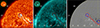 |
Fig. 2. Images taken from JHelioviewer corresponding to the source of the CME event prior to the eruption at 13:48:20 on July 9, 2013. The left panel shows the image of the solar atmosphere in Solar Dynamics Observatory/Atmospheric Imaging Assembly 304 Å wavelength, where the circles identify the footpoints. The middle panel shows the solar corona in SDO/AIA 131 Å wavelength, with a dotted sigmoid shape plotted on top. The right panel shows the HMI magnetogram with the red line corresponding to the polarity inversion line (PIL) together with the dotted sigmoid and the footprints plotted on the left and middle panels. |
The CME event was observed by the STEREO-A and STEREO-B coronagraphs and in situ by MESSENGER near Mercury and ACE near Earth. The locations of STEREO-A, STEREO-B, Mercury, and Earth are given in Figure 3. The angular separation between MESSENGER and ACE at that time is only 3.1° (Salman et al. 2020).
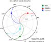 |
Fig. 3. Alignment of the Mercury and Earth at the time of the CME eruption. The locations of STEREO-A and STEREO-B are also plotted. The figure is generated with Solar-MACH (Gieseler et al. 2023). |
The images observed by the coronagraph instruments on the STEREO-A and STEREO-B after ∼3 hours from the CME eruption are plotted in Figure 4. The panels are generated with the Stereo CME Analysis Tool (StereoCAT) at the Community Coordinated Modeling Center.
 |
Fig. 4. White-light images seen from STEREO-A C2 and STEREO-B C2 ∼3 hours after the CME eruption. The figure was generated with the Stereo CME analysis tool. |
The CME was fitted with the online tool available on the StereoCAT website to estimate the direction of the CME, its angular width, the speed of propagation, and its arrival time at 0.1 au. The initially estimated CME parameters were used as the starting point for the 3D reconstruction with the Graduated Cylindrical Shell (GCS) model (Thernisien 2011). The obtained parameters for injecting the CME at 0.1 au in the heliosphere are given in Table 2. As Palmerio et al. (2018) describe, the tilt was estimated from in situ measurements to be ∼10° with the axial direction to the west and the flux rope type of NWS, in comparison to the estimated tilt of 50° with the axial direction to the southwest and the flux rope type of WSE/NWS from the solar disc appearance. Therefore, we also fixed the tilt to 10° in the simulations and later investigated the difference between two models with the same parameters, but the tilt fixed to 45° and 10° degrees, respectively.
Parameters for the input for the spheromak CME model for the event on July 9, 2013.
3.2. Comparison of simulations to data
First, the background solar wind was simulated in the heliosphere. The WSA coronal model of EUHFORIA was used to obtain the plasma conditions at 0.1 au. The Global Oscillation Network Group (GONG) magnetogram corresponding to 2013-07-09T13:14:00 was used for computing the coronal model. After a relaxation period of 14 days, the spheromak CME model with the parameters described in Table 2 was injected. The time series modelled at different planets and spacecraft are generated while obtaining the modelled 3D heliosphere. The time series obtained at Mercury and Earth are used to compare with the observed data.
Figure 5 shows the time series of the magnetic field components near Mercury. The blue line corresponds to the observed data by the MESSENGER spacecraft. As MESSENGER was originally designed to study the magnetosphere of Mercury in more detail, it spends a significant amount of time inside the magnetosphere of the planet. The magnetic field of Mercury is rather strong. Therefore, the times when the satellite is affected by the magnetic field of the planet are removed from the observed time series. The nearest magnetopause crossing is estimated to be ∼1 − 2 hours from the spacecraft’s passage through the plasma sheet, during which the plasma parameters and the magnetic field are expected to change (Sun et al. 2022; James et al. 2017). The average crossing length from the magnetometer observations was estimated to be ∼3.5 hours.
 |
Fig. 5. Simulations performed with different numerical grids in Icarus. The blue line corresponds to in situ data observed at the MESSENGER spacecraft. Magnetic field components are plotted. The black, red, and green lines indicate shock arrival time, the ME LE, and the ME TE, respectively. Equidistant grid simulations on the low and medium-resolution grids are given in orange and green. The simulations performed on the stretched grid with AMR levels 2, 3, and 4 are given in red, purple, and brown, respectively. |
The dashed black, red, and green vertical lines indicate the arrival of the disturbance at MESSENGER, followed by the arrival of the magnetic ejecta leading edge (ME LE) and the passing of the magnetic ejecta trailing edge (ME TE), according to Winslow et al. (2015). However, the arrival of the shock and the ME LE fall in the period of the magnetosphere passing, which is associated with high spikes in the magnetic field, but does not indicate the arrival of the magnetic cloud. Therefore, the time inside the magnetosphere crossing interval cannot be considered as the arrival time of the CME at MESSENGER. The strong variations in the magnetic field components and increased total magnetic field at ∼22:00 on July 10, could indicate the arrival of the CME sheath (Burlaga et al. 1982).
The results from simulations in Icarus performed on different grids are presented with different curves. The orange and green curves correspond to simulations performed on the low and medium-resolution computational grids, while red, purple, and brown curves correspond to simulations performed on the stretched grids in combination with AMR refinement levels 2, 3, and 4, respectively. The AMR criterion is the same in all simulations, as described in Section 2.
Because of the strong noise in the MESSENGER data and the magnetosphere passing at the possible start of the CME arrival at the planet, a detailed comparison of the modelled and observed data is challenging. However, we see that the polarity of the simulated magnetic field for all components is in agreement with the observed data. The strength of the positive Bz component is modelled poorly, as it seems higher in the observed data. However, the negative values of this component are modelled well. The profile of the simulated total magnetic field strength resembles the observed profile. The simulated Bx and By components vary rather smoothly in time, and no strong variations are present. The advantage of applied AMR can be seen in the profiles of By and the total magnetic field strength at the effective arrival of the magnetic cloud in the simulation. The small peak before the arrival of the magnetic cloud is better resolved in the AMR level 3 simulation than in the equidistant medium-resolution simulation and is more similar to the observational data. The feature in AMR level 4 simulations is sharper than in all other simulation results and shows more variations as MESSENGER passes through the magnetic cloud.
Figure 6 shows the plasma and magnetic field parameters at ACE. The colour choices are similar to the previous figure, the observed data is plotted in blue, and the arrival of the disturbances, ME LE and ME TE, are plotted with black, red, and green vertical dashed lines, respectively. The left panel focuses on plasma parameters and plasma−β in the simulation. when considering the arrival time the speed profiles are modelled well, but the number density peaks slightly earlier than in the observation data. The shock in the speed values is steeper in AMR level 3 and 4 simulations than in the equidistant medium-resolution simulation. The value of the plasma beta indicates that the magnetic cloud arrival is in good agreement with the observed data. In this panel, we can see the two-peak structure in AMR level 4 simulation, which can be connected to the peaks at the arrival of the disturbances at Earth and the arrival of the magnetic cloud. The two peaks are also present in the equidistant medium-resolution simulation, but the first peak is stronger than the second one, in this case.
 |
Fig. 6. Simulations performed with different numerical grids in Icarus. The blue line corresponds to in situ data observed at the ACE spacecraft. On the left panel the radial velocity, number density, and logarithm of plasma-β are plotted. The right panel shows the magnetic field components and the total magnetic field. The shock arrival time, the ME LE, and the ME TE are indicated in the catalogue from Winslow et al. (2015) and are plotted with black, red, and green dashed lines, respectively. Equidistant grid simulations on the low- and medium-resolution grids are given in orange and green. The simulations performed on the stretched grid with AMR levels 2, 3, and 4 are given in red, purple, and brown, respectively. |
On the right panel of Figure 6, we can see that the simulated Bx component of the magnetic field closely resembles the profiles in the observed data. In the case of the By and Bz components, the overall profiles are similar in the modelled and observed data, but the profiles in the magnetosheath and beginning of the ME seem to be compressed in the modelled data, not catching the exact profile of the observed data. In the simulation study, it was observed that the magnetic cloud arrived a bit later in the equidistant medium-resolution simulation. This delay could be explained by the fact that the shock arrival in the radial velocity panel was less steep, indicating a gradual increase compared to other simulation runs. This indicates that the front of the CME is more diffuse in the equidistant simulations than in the other simulations and the sheath region is modelled more poorly. When considering the total magnetic field panel, the increased strength in the sheath region can be distinguished well in AMR level 3 and 4 simulations, with AMR level 4 results being slightly more similar to the observed data. The stronger magnetic field region arrives later in the equidistant medium-resolution simulation and appears to be narrower than in the AMR simulations and the observed data. The strength of the total magnetic field is underestimated in the simulation results.
Overall, the CME interaction at Mercury and Earth is modelled well, considering that the arrival time and the strengths of the variables and profiles are in good agreement with the observed data at Mercury by the MESSENGER spacecraft and near Earth by the ACE spacecraft. Grison et al. (2018) reported that no significant acceleration or deceleration was calculated for this CME event. From the simulations, we could also see that at both locations it arrived close to the arrival time reported in Winslow et al. (2015) and Salman et al. (2020). When comparing the magnetic field components at two different locations, we can see no significant change in the orientation of the magnetic field configurations, which indicates that the two spacecraft passed through the CME at similar locations and no significant rotation and deflection took place from the orbit or Mercury to the orbit of Earth.
When considering different computational grids for modelling the solar wind and the CME, we can see that near Mercury, the equidistant medium-resolution simulation result is more similar to the AMR level 3 simulation results, when comparing the resolved small variations in the time-series. The AMR level 4 simulation resolves the structure of the magnetic field upon its arrival in more detail than the other simulations and performs better than the equidistant medium-resolution simulation.
Figure 7 shows the results from the Icarus simulation performed on the stretched grid in combination with AMR refinement level 4. The snapshots are taken in the equatorial plane at the arrival time of the CME shock at 1 au. The white dashed line is along the Sun-Earth line and the Earth icon is placed at the location of Earth in the given snapshot. The frame is rotated so that Earth is fixed at 0° longitude. The left panel represents the magnetic field strength with the given colour bar in [nT]. The middle panel represents the CME density values, saturated to (0, 0.1) in the code units, for better visibility. The density profile is overlaid by the divergence of ⃗V values, showing the compression regions in the domain. The values are saturated to ( − 0.1, 0.1) to better distinguish the compression regions, given in red. Thus, from this panel, we can see the whole structure, the red shock front, and the CME interior behind it. The right panel represents the same values plotted as in the middle panel but with the computational grid plotted on top. The same portion is plotted from the equatorial plane without zooming for consistency. The dense region corresponds to AMR level 4 covering most of the CME interior and the CME shock front, as indicated in the AMR refinement criterion.
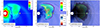 |
Fig. 7. Equatorial plane in Icarus at the arrival time of the disturbance at 1 au. The distance from the Sun is indicated on the horizontal and vertical axes. The left panel shows the slice coloured with total magnetic field values. The middle panel shows the plasma density inside the CME overlaid with the divergence of velocity values. The right panel shows the medium panel with the computational grid plotted on top. The frame is rotated so that Earth is fixed at 0 longitude. The white dashed line is along the Sun–Earth line. |
Finally, we performed a simulation with the tilt that was calculated from the PIL line at the solar photosphere and compared it to a simulation using the tilt deduced from the in situ measurement by Palmerio et al. (2018). Figure 8 shows the time series at Mercury (left panel) and at ACE (middle and right panels). Both simulations were performed on the stretched grid with 4 AMR levels, as these simulations resolve more small-scale structures in time series than others. The orange curve corresponds to the parameter setup given in Table 2, with tilt = 10°, while the green curve corresponds to the simulation with tilt = 45°. At Mercury, we can see, the Bx component is overestimated in the simulation with tilt = 45°. The By component is comparable to the standard tilt simulation, but the magnetic cloud seems less extended.
 |
Fig. 8. Observations at Mercury and ACE plotted in blue similar to Figures 5 and 6. The left panel represents magnetic field components at MESSENGER and the middle and right panels show those at ACE. The orange curve corresponds to the same parameter setup as reported previously, with the tilt = 10° and green corresponds to the same parameter set, apart from tilt = 45°. The simulations are performed on an AMR level 4 grid. |
The Bz component is underestimated compared to the simulation results with tilt = 10°. Overall, at Mercury, the simulation with tilt = 10° produces results that are more similar to the observed data than with tilt = 45°. At ACE, the profiles corresponding to the simulations with tilt fixed to 10° and 45° are more similar and no significant difference can be spotted. When comparing the magnetic field component profiles at Mercury and ACE, we can see that there is a larger difference in the case of the simulation with tilt = 45°, especially in the By and Bz components, which can be explained to the rotating feature of the spheromak model in the simulation (Asvestari et al. 2022; Maharana et al. 2023; Sarkar et al. 2024). This indicates that the rotation of the flux-rope occurred in the solar corona or the lower heliosphere, below ∼0.35 au, since the magnetic field components are better recovered by the simulation with the tilt fixed to 10° at both locations in the heliosphere.
Table 3 shows the wall-clock times for the different Icarus simulations all performed on 4 nodes on the Genius cluster at KU Leuven. Each node contains 2 Xeon Gold 6240 CPUs@2.6 GHz (Cascadelake), 18 cores each. The equidistant medium-resolution simulation took the longest as expected, ∼1 h 14 min. The AMR level 4 simulation, which produced comparable or better results when looking at time series data, took only ∼35 minutes, which is ∼2.1 times faster than the equidistant medium-resolution simulation. The AMR level 3 simulation took under 8 minutes, similar to low-resolution simulation while showing considerably more small-scale features in the time-series data. Thus, performing simulations with the combined refinement criterion, which aims at a large area is still more advantageous than using the standard equidistant grid without optimization.
Wall-clock times for the performed simulations in Icarus.
4. CME event II: February 16, 2014
4.1. Observations of the studied CME
For the second analysed event we chose the CME which occurred on February 16, 2014, at 10:24 UT, as reported by Winslow et al. (2015) and Salman et al. (2020). The CME was observed at MESSENGER on February 17, 2014, at 04:17, and at ACE on February 19, 2014, at 03:48. The corresponding spacecraft longitudinal separation was 4.8°. The source was identified in the solar atmosphere, corresponding to the active NOAA 11977, and the M1.1 class flare occurred at 09:00 UT with the peak at 09:26 am with coordinates S10E00. The snapshots of the region before the eruption are given in Figure 9. The left figure shows the AIA 304 Å wavelength filter, where possible foot-points are encircled in blue. The middle panel shows AIA 131 Å to distinguish the sigmoid structure better. The approximated S-shaped sigmoid is plotted with the red dotted line at the eruption site. The sigmoid’s orientation means that the eruption’s chirality is positive. Therefore, the flux-rope magnetic field configuration is right-handed. The right panel shows the HMI magnetogram with the PIL plotted on top, the approximated sigmoid structure, and the footprint sites for the whole picture. The PIL suggests that the axial direction is northwest, and the flux rope is WNE/SWN type. The tilt calculated from the PIL is ∼59.6°.
 |
Fig. 9. Images taken from JHelioviewer corresponding to the source of the CME related to the eruption at 09:22:11 on February 16, 2014. The left panel shows the image of the solar atmosphere in SDO/AIA 304 Å wavelength, where the circles identify the footpoints. The middle panel shows the solar corona in SDO/AIA 131 Å wavelength, with a dotted sigmoid shape plotted on top. The right panel shows the HMI magnetogram with the red line corresponding to the PIL together with the dotted sigmoid and the footprints plotted on the left and middle panels. |
The CME event was observed by MESSENGER and ACE, and their locations, together with Stereo-A and Stereo-B, are plotted in Figure 10. The angular separation between Mercury and Earth is slightly larger (by 1.7°) here than for the previous CME event studied. The CMEs were not well distinguishable in the available coronagraph images. Nevertheless, the signatures can be seen in Stereo-A C2 and SOHO/LASCO C3 images, given in Figure 11. The CME is encircled in white, and the leading parts are indicated by a white arrow. The white-light images from Stereo-B did not contain good enough images to distinguish CME contribution. Therefore, they are not plotted. The snapshots in Figure 11 are taken after ∼2.5 hours since the launch of the CME from the solar atmosphere. Therefore, the CME has already expanded in the C2 image and can already be seen in C3. Since the CME cannot be distinguished very well, obtaining parameters from StereoCAT and GCS fitting was challenging. The obtained parameters were used as initial guesses and further optimised when comparing the modelled data to the observed data.
 |
Fig. 10. Alignment of the Mercury and Earth at the time of the CME eruption. The locations of STEREO-A and STEREO-B are also plotted. The figure is generated with Solar-MACH (Gieseler et al. 2023). |
 |
Fig. 11. The white-light images seen from STEREO-A Cor2 and SOHO/LASCO Cor3 ∼2.5 hours after CMEC eruption. The figure is generated with the Stereo CME Analysis Tool. |
4.2. Three interacting CMEs
However, when injecting only this single CME in the heliosphere, the synthetic time series poorly matched the in situ data, missing prominent features in the data. The catalog by Richardson & Cane (2024) indicates CMEs registered at Earth (L1) before and after this CME. According to this catalog, the registered disturbances on Earth are given in Table 4. CMEP, CMEC, and CMEA stand for the previous CME, the current CME, and the CME that arrives after, respectively. From this table, we can see that the arrival of the disturbance for the second CME is before the ME of the first one has passed Earth. Therefore, there is a CME-CME interaction occurred before 1 au.
CMEs registered at Earth in the catalogue by Richardson & Cane (2024).
The third CME arrival time is right after the second one (CMEC) has passed Earth. This indicates a second CME-CME interaction along the way, and the third CME compressed the second CME. Since with the isolated second CME modelling the time series did not replicate any of the prominent features in the observed data, we also modelled the other two CMEs, resulting in a heliospheric simulation with three consecutive CMEs being injected from the inner boundary.
The source of the preceding CME was not identified, which was also reported in the study by Wang et al. (2018). We estimated the CME parameters to model it at 0.1 au from the in situ data to reconstruct the plasma conditions before the arrival of CMEC. The CME must have had low speed, as upon its arrival at Earth, the speed increases suddenly from ∼350 km s−1 to ∼420 km s−1 (Figure 12). The CME speed profile is flat. The ME arrives 8.5 hours later, and it takes 15 hours to pass ACE according to Table 4. However, the in situ data reveal that after the arrival of the magnetosheath of the second CME, there is a slight variation in the plasma−β profile. But the ME ended passing ACE at 15:00 am from Figure 12, meaning the passage took 21 hours. The magnetic field strength does not significantly increase since it remains under 10 nT throughout the ME passage while it reaches ∼20 nT in the preceding sheath. Considering the orientation of the magnetic field components, a left-handed CME configuration was assumed with 0° tilt.
 |
Fig. 12. Simulations performed with different numerical grids in Icarus. The blue line corresponds to in situ data observed at the ACE spacecraft. The radial velocity, number density, and logarithm of plasma-β are plotted on the left figure. The right figure shows the magnetic field components and the total magnetic field. The shock arrival time, the ME LE, and the ME TE are indicated in the catalogue from Winslow et al. (2015) and are plotted with black, red, and green dashed lines, respectively. The solid vertical magenta and blue lines indicate the arrival of the shock disturbances of the previous and following CMEs on Earth. Equidistant grid simulations on the low and middle-resolution grids are given in orange and green. The simulations performed on the stretched grid with AMR levels 2, 3, and 4 are given in red, purple, and brown, respectively. |
On the other hand, the third CME, CMEA, was found in The Space Weather Database Of Notifications, Knowledge, Information (DONKI) catalog of CCMC with estimated direction, size, and propagation speed. According to the parameters reported in the DONKI catalog, the CME was launched at (ϕ, θ) = (−29 ° , − 19 ° ) in HEEQ coordinates with a speed of Vr = 600 km s−1 and a half angular width ω/2 = 53°. The CME reached 0.1 au, the inner heliospheric boundary, at 07:32 on February 18, 2014. Since these parameters were obtained for the simple hydrodynamics plasma CME model, the parameters were fitted with the StereoCAT online tool and GCS 3D reconstruction and further optimised in the simulations. The aim of including the third CME in the simulation is to investigate its effect on the main CME we are modelling. The CME was visible at STA, SOHO/LASCO, and STB, as shown in Figure 13. As can be seen from these figures, CMEA is large and has a high speed since the snapshots are taken only ∼1.5 hours after the CME launch. After performing the fitting of the CME with the StereoCAT online tool, the obtained (ϕ, θ) = (−10 ° , − 36 ° ) in HEEQ coordinates with the speed of Vr = 950 km s−1 and half angular width ω/2 = 43°. We located the source on the solar photosphere to identify the orientation of the flux rope and estimate the tilt for the input spheromak CME model. Figure 14 shows the source region before the eruption. In all three figures, the location of the eruption is indicated with a white circle. The left figure is made through the AIA 304 Å wavelength filter. The middle figure shows the solar corona through the AIA 131 Å filter. The right figure shows the HMI magnetogram. The possible PIL locations are over-plotted with red solid lines at the possible eruption site. The exact CME source was hard to identify since the eruption can only be seen near the limb. The images in the AIA 131 Å and AIA 304 Å filters are blurry, and it is hard to distinguish the pre-eruptive structures to identify the tilt and exact helicity of the flux-rope. We started with the PIL tilt shown in the figure and further optimised it in the simulations. Since the goal of including the third CME was only to check its effect on the second one and whether it compresses the previous one, further identification of the source of the third CME was not pursued. The obtained parameters are given in Table 5, which were used for modelling CMEs in the heliosphere.
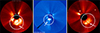 |
Fig. 13. The white-light images seen from STEREO-A Cor2, SOHO/LASCO Cor3 and STEREO-B C2 ∼1.5 hours after the CMEA eruption. The figure is generated with the Stereo CME Analysis Tool. |
 |
Fig. 14. The images taken from JHelioviewer correspond to the source of CMEA event before the eruption at 01:21:26 on February 18, 2014. The left and right panels show the images of the solar atmosphere in Solar Dynamics Observatory/Atmospheric Imaging Assembly 304 Å and 131 Å wavelengths, respectively. The white circle highlights the filament area. The right panel shows the HMI magnetogram with the red lines corresponding to the polarity inversion lines (PIL) found in the filament region. |
The parameters for the input for the spheromak CME model for the three CMEs for February 16, 2014.
4.3. Comparison of simulations to data
Figure 15 shows the time series obtained at MESSENGER. The MESSENGER data are plotted in blue. The data from passages of the magnetosphere are removed as the CME contribution cannot be distinguished there from the strong magnetosphere magnetic field. The black, red, and green vertical dashed lines indicate the arrival of the disturbance, ME LE and ME TE at MESSENGER reported in Winslow et al. (2015), respectively. Unfortunately, MESSENGER enters the magnetosphere of Mercury within 2 hours from the arrival of the ME, so more than half of the CME contribution cannot be distinguished from the observed data. This increases the ambiguity when comparing the modelled data to the observed data. In the left figure, the equidistant grid simulation results with the low and middle-resolution grids are plotted with orange and green, respectively. The results for AMR level 2, 3, and 4 simulations on stretched grids are plotted with red, purple, and brown colours, respectively. The right-hand side figure plots the AMR level 4 simulation result in the solid magenta line. The synthetic data was shifted artificially by 13 hours back in time to match the arrival time in the observed data to allow better comparison of the magnetic field components to the MESSENGER observations. The shifted synthetic data is plotted with the dashed magenta line.
 |
Fig. 15. Simulations performed with different numerical grids in Icarus. The blue line corresponds to in situ data observed at the MESSENGER spacecraft. The black, red, and green vertical dashed lines indicate the shock arrival time, the ME LE, and the ME TE, respectively. The left figure shows magnetic field components. Equidistant grid simulation results with low and medium-resolution grids are given in orange and green. The results of the simulations performed on the stretched grid with the combination of AMR levels 2, 3, and 4 are given in red, purple, and brown, respectively. The right figure shows the shift of the modelled data in time with 13 hours to project the profiles during the CME interaction at MESSENGER. |
The CME arrives later than in the observed data in the simulation results. The time delay is 10 − 13 hours, depending on the resolution of the simulation. Grison et al. (2018) describes the deceleration of the CMEs beyond the Mercury orbit until 1 au. In this case, the CME deceleration was significant, as from ballistic measurements of the CME speed, the CME transit speed from the Sun to Mercury was estimated to be ∼820 km s−1, and the average CME transit speed from Mercury to Earth was estimated to be ∼570 km s−1 (Salman et al. 2020). In the simulation, this deceleration was not recovered. Therefore, the arrival times at the two locations were not accurate. Since the observed data was of low quality and mostly missing at Messenger, we fixed the parameters to match the arrival time at Earth. Thus, we get a significant delay in the synthetic data for the CME arrival at MESSENGER. For more accessible comparison purposes on the right panel in Figure 15, we shifted the synthetic data by 13 hours, as mentioned. We only plotted the results of one simulation corresponding to AMR level 4 so as not to overload the figure. This figure shows that the polarities of the magnetic field components match the observed data. The negative values of the Bz component are not reconstructed well, and the strength of the positive values is similar to the observed data.
The left panel of Figure 15 displays results computed on different simulation grids. The low resolution and AMR level 2 simulations show similar smooth profiles. The AMR level 3 simulation already indicates results comparable to the equidistant medium-resolution simulation. The AMR level 4 simulation result demonstrates the sharpest profiles when changing the magnetic field polarities, which can also be seen in the total magnetic field strength profile. Unfortunately, further comparison of the synthetic data with the observations at MESSENGER is difficult, as most of the observed data is missing. Therefore, the passing of the ME is ambiguous since it coincides with the period when the MESSENGER is located within the planet’s magnetosphere.
Figure 12 shows the time profiles at ACE. The observational data by ACE are plotted in blue, and the vertical dashed black, red, and green lines represent the arrival of the shock disturbance, ME LE and ME TE at Earth, respectively, for CMEC. The arrival times for the shock and the passing of the ME are the same as indicated in Winslow et al. (2015). However, the arrival of the ME was shifted from the reported 12:00 to 14:34, as the plasma variables in these ∼2.5 hours have more of a sheath structure than of the ME. The plasma-β and magnetic field components fluctuate, usually characteristic of the sheath region. After the newly identified arrival of the ME, the ME has more homogeneous profiles, and plasma-β values start to decrease, indicating the domination of the magnetic forces over the plasma pressure force.
In Figure 12, the solid vertical magenta and blue lines indicate the arrival of the sheath of the previous and following CMEs, indicated with CMEP and CMEA. Since the shock of CMEA arrives shortly after the passage of the ME TE of the CMEC, they appear very close on the figure, but the lines can be distinguished.
At the magenta vertical line, corresponding to the arrival of CMEP in the simulation, we can see a slight increase in the speed profile, comparable to that in the observational data. The enhancement in the number density profiles is also localised around this vertical magenta line. In contrast, in the observational data, the main increase in the number density arrives later at ACE. The plasma-β values indicate the arrival of the ME shortly after the arrival of the magneto sheath region, which is in good agreement with the observed data. The modelled magnetic field components agree with the observations for the first CME. The strength of the total magnetic field is also similar to the one observed, guaranteeing good background conditions upon the arrival of the following CME, which is the main CME we are modelling in this study. The profiles in this region are smooth. Therefore, no significant advantage can be seen in any of the different simulations regarding the sharpness of profiles or resolving more small-scale structures.
The arrival time for the second CME, indicated by CMEC on the figure, is similar in the synthetic modelled data and the observations. However, the solar wind profile is overestimated before the arrival by ∼40 km s−1. The shock jump is calculated by the following formula Vjump = VP − VSW, where SW stands for the solar wind before the arrival of the disturbance and P stands for the peak value upon the arrival. From this calculation, the speed jump in the observational data is ∼105 km s−1, while in the synthetic data from the simulation, it corresponds to ∼210 km s−1. Therefore, the speed upon the arrival of the CME is strongly overestimated, which indicates that the deceleration is not very well modelled in Icarus.
When the ME arrives at ACE, there is a further increase in the speed values in the observed data by ∼60 km s−1. Then, the profile of the speed is flat while passing by ACE, while in the synthetic data from the simulation, the speed values decrease towards the tail of the CME, obtaining similar values at the ME TE. This could indicate that the CME was more compressed in the observed data by the third CME, not allowing it to expand, while the compression was not reconstructed to the same extent in the modelled data.
The number density modelled by Icarus agrees with the observed data. In plasma-β values, we can see that the values in the modelled data start to decrease, similar to the observed data, where the arrival of the ME LE is indicated. However, we see that in the observed data, the values start to increase at the ME rear, which is not the case in the modelled data. This indicates that the third CME has not compressed the second one as much in the simulation as in the actual scenario.
When considering the total magnetic field strength (Figure 12, left bottom panel), there is a substantial increase upon the arrival of the shock of the second CME. This results from the CME-CME interaction occurring from the orbit of Mercury onwards to 1 au, as the shock of the second CME travels through the ME of the first one. This region is slightly more compressed in the modelled data than in the observations. Still, all magnetic field components are very similar to the observed data, apart from the By component, for which the negative region is more expanded, and the positive region seems more compressed and arrives later. The magnetic field values before the arrival of the ME are in agreement with the observations. The ME arrives at the red vertical dashed line in Figure 12, both in the simulations and observation data. The modelled and observed profiles of the magnetic field components are similar. In the simulation results, the profiles seem more “stretched”, caused by a weaker interaction with the third CME.
The simulated third CME, CMEA, arrives simultaneously as in the observed data. Only the first part of the third CME is plotted, as analysing the third CME in detail exceeds the scope of this paper. Because of the over-expanded second CME, we obtain a CME-CME interaction between the second and the third CME, which is much smaller in the observed data. The speed values are in good agreement between the observed and modelled data in the front part of CMEA; however, later on, the simulated CME is much faster. The plasma−β values are slightly lower, and the total magnetic field is also stronger in the simulations than in the observations in the front part of CMEA, while it is the reverse later on.
The interactions with the other CMEs were not captured well with a smaller radius for the second CME. The reason for the over-expanded second CME and insufficient compression can be a characteristic of the spheromak CME model, which usually is more radially expanded than in the observations (Scolini et al. 2019).
The separation between the spacecraft during this CME case was 4.8°, which is slightly larger than in the first case. When comparing the magnetic field components, the polarities are in good agreement for By and Bz, but are different for the Bx component, which the longitudinal separation between the spacecraft could cause.
The refinement criterion was the same as in the first CME case reported in Section 3, with only one difference, as we fixed a slightly larger margin for the latitudinal direction to allow more refinement. Upon the arrival of the second CME, the shock jump in the speed values is the sharpest in the simulation performed on the medium-resolution equidistant grid and in the AMR level 4 simulation (Figure 12). The AMR level 3 results are similar to the AMR level 2 simulations regarding smoothness. The third CME arrives at the latest in the AMR level 4 simulation, but the profile is very similar to that from the medium equidistant simulation. Therefore, we can see that the features are well resolved at Mercury with AMR level 3 simulation. In contrast, at Earth, the profiles modelled with AMR level 3 are relatively smooth, and an additional refinement level is required to see smaller structures.
Figure 16 shows the simulation results in the equatorial plane crossing Earth, showing the strength of the magnetic field in nT. The three snapshots are taken at the arrival times at 1 au for CMEP, CMEC, and CMEA, respectively. The simulation output is saved only every 3 hours. Therefore, the snapshot closest to the arrival times is plotted. All three snapshots are within 1 hour from the observed arrival time reported in Table 4. The simulation is performed on an AMR level 4 grid. This figure shows the increase in the total magnetic field regions upon the arrival of the second and third CMEs. In the middle and right panels, we can see the CME-CME interactions between the first and second CME pairs and the second and third CME pairs, respectively.
 |
Fig. 16. The snapshots represent the equatorial plane in Icarus. The slice is coloured with B – total magnetic field values in [nT]. The distance from the Sun is indicated on the horizontal and vertical axes. The left figure represents a snapshot taken at the arrival time of the first CME on Earth. The second CME represents the snapshot corresponding to the arrival of the second CME, and the third one denotes the magnetic field configuration upon the arrival of the third CME. The timestamps are indicated on each snapshot. The frame is rotated so that Earth is fixed at 0 longitude. The white dashed line is along the Sun-Earth line. |
Table 6 shows the run times for the simulations performed in Icarus. All simulations are performed on four nodes on the Genius cluster at KU Leuven. The medium-resolution simulation is 8 and 1.9 times slower than the simulation with the stretched grid and AMR levels 3 and 4. AMR level 3 produces results similar to the medium equidistant simulation at Mercury, and AMR level 4 performs similarly to the medium-resolution simulation on Earth. Therefore, depending on the purpose of the simulation, the maximum refinement level can be chosen accordingly.
The wall-clock times for the performed simulations in Icarus.
4.4. Timing tests
Figure 17 compares the time performance of the two types of simulations. The highest resolution simulations, the AMR level 4 run on a stretched grid and the medium-resolution simulation on an equidistant grid, were performed on 1, 2, 4, and 8 nodes with 2 Xeon Gold 6240 CPUs@2.6 GHz (Cascadelake), 18 cores each, on the Genius cluster at KU Leuven. The AMR level 4 and medium-resolution simulation times are marked with red triangles and blue squares, respectively. When both simulations are performed on one node, AMR level 4 simulation is 3.5 times faster; on two nodes – 2.9 times faster; on four nodes – 1.88 times faster; and on eight nodes – 1.3 times faster.
 |
Fig. 17. The timing tests for the medium-resolution simulation on the equidistant grid and the AMR level 4 simulation on the stretched grid. The horizontal axis denotes the number of nodes, and the vertical axis denotes the wall clock time in hours. The simulations are performed on the given amount of nodes with 2 Xeon Gold 6240 CPUs@2.6 GHz (Cascadelake), 18 cores each, on the Genius cluster at KU Leuven. |
Additionally, we calculated that performing the medium-resolution simulation on four nodes speeds up simulations by a factor of 4.1 compared to the performed simulation on one node. In contrast, for the AMR level 4 case, the simulation on four nodes is 2.2 times faster than on one node. The medium and AMR level 4 simulations performed on eight nodes are 7.95 and 3 times faster than those performed on one node. Therefore, the efficiency gain when running with additional nodes decreases with more AMR levels than in the medium-resolution equidistant simulation. Nevertheless, the simulations performed on the stretched grid with AMR level 4 are faster than those with the medium-resolution simulation on the equidistant grid while resolving similarly or better the small-scale features in the variations of the time series of the modelled quantities.
5. Conclusions
We validated the magnetised linear force-free spheromak model newly implemented in the optimised heliospheric wind and CME evolution tool Icarus. To do so, we selected two CME events that were observed by two spacecraft, namely MESSENGER and ACE.
There were multiple reasons to choose these particular events. First, the CME events observed by MESSENGER and ACE are favourable because the radial separation between the orbit of Mercury and Earth is large, and ranges between 0.55 and 0.65 au, depending on the location of the planets. This allows a comparison of the performance of the code close to the inner boundary of the computational domain and farther out in the middle of the domain (in the radial direction).
The events were chosen from the catalogue described in Winslow et al. (2015) and have already been further analysed by Grison et al. (2018). From the listed events, we chose one that represents a quiet case, with a clearly defined CME shock and magnetic cloud, and a second one where more complex interactions are observed. The first of these events occurred on July 9, 2013, and the second on February 16, 2014.
We identified the source region for the first CME event and obtained the parameters for modelling the CME with the geometrical fitting on the StereoCAT online tool and 3D GCS reconstruction. We then injected the spheromak CME model in Icarus with the determined parameters. The synthetic (modelled) data at the locations of Mercury and Earth were compared to the observed data by MESSENGER and ACE. The periods MESSENGER spent in Mercury’s magnetosphere were removed from the time series. However, the arrival time of the CME at MESSENGER coincided with the spacecraft passing through the planet’s magnetosphere. Therefore, this cannot be considered the start of the magnetosheath of the CME at MESSENGER. The spacecraft goes through the magnetosphere of Mercury two more times until the passing of the trailing edge is registered at MESSENGER; therefore, the data are incomplete. Still, Icarus modelled the polarities of the magnetic field components in agreement with the observed data. Unfortunately, MESSENGER does not observe plasma conditions, such as speed, number density, and temperature, and hence complete validation of all states is impossible.
Further, we investigated the effect of the CME at ACE. We modelled the arrival time of the CME and find it to be in agreement with the observed data; the modelled magnetic field components also replicate the strength values and polarity signs of the observed data. As reported by Grison et al. (2018), no significant deceleration or acceleration was obtained for this CME event. The modelled arrival at both locations agrees with the dates reported in Winslow et al. (2015) and Salman et al. (2020). The simulation performed using the AMR level 4 grid resolves the small-scale signatures on Earth, while at Mercury, the profiles are rather smooth, and we see no significant advantage of using AMR. The AMR level 3 and 4 simulations are, respectively, ∼9.5 and 2.1 times faster than the medium-resolution equidistant grid simulation, even though the results modelled with the AMR level 3 and 4 simulations are similar or slightly better than the medium-resolution simulations on the equidistant grid.
The second CME case is more complex, as the catalogue by Richardson & Cane (2024) registered other CMEs before and after the chosen CME. We identified the source of the second CME event and obtained the CME parameters again through StereoCAT and GCS fitting. The coronagraph images do not provide sufficiently high-quality data, and the CME contributions are faint. Therefore, we further optimised the CME parameters with heliospheric modelling. However, we were not able to reconstruct the time series profiles by modelling the isolated CME in Icarus.
The conditions prior to the arrival of the CME are significantly different in the simulations, and the CME is overexpanded. Therefore, the preceding and following CMEs were taken into account in the Icarus model. The source of the preceding CME cannot be identified, as the CME is slow and extended. We estimated the parameters for the injection at 0.1 au, the inner heliospheric boundary, to reconstruct the conditions before the arrival of the CME of our choice. Next, the source region for the third CME was located. A large filament was observed with multiple ribbons, but we were not able to identify the exact source for the ejected flux rope. The tilt of the spheromak was further optimised with the heliospheric simulations. As the aim of including the third CME is to investigate its effect on the propagation of the main CME in the event, the parameters of the third CME were not optimised in detail.
In summary, we modelled the second CME event by injecting three CMEs into Icarus. The CME–CME interaction between the preceding and the main CME was well reconstructed and the arrival signatures were captured in the heliospheric simulation. The main CME is more expanded in the Icarus simulation than in the observations. Therefore, the interaction between the second and third CMEs is underestimated in the simulation results compared to observations. However, we note from the observations that the presence of the third CME still compressed and pushed the second CME, compared to simulations where the third CME was not modelled. We also find the choice of CME density for injecting the CMEs to be important, as it has a large effect on whether or not the plasma cloud is contained.
Overall, we note that lower AMR levels are sufficient at the orbit of MESSENGER to distinguish smaller-scale features, while higher levels of AMR are needed at ACE. This is due to the nature of the stretched grid, as the cell sizes are naturally smaller at the orbit of Mercury than at the orbit of Earth. The best results were obtained with AMR level 4 at ACE, while at Mercury AMR level 3 results were already similar to equidistant medium-resolution simulations. This implies that when choosing recent missions for sampling the heliosphere, lower AMR levels are sufficient to obtain sufficiently detailed time series when the spacecraft is close to the inner heliospheric boundary.
We also analysed the simulation wall-clock times. The AMR level 3 and 4 simulations are 8 and 1.88 times faster than the medium-resolution equidistant simulation runs, respectively. The AMR simulations are slightly slower than in the previous CME case, as three CME are modelled, and a considerably larger part of the computational domain needs to be refined.
Finally, we performed timing tests for the AMR level 4 and medium-resolution simulations. For this purpose, we performed simulations on 1, 2, 4, and 8 nodes on the same cluster at KU Leuven. The results indicate that a large number of nodes is not beneficial for the given size of the simulations.
In summary, we successfully modelled the two CME events with the new heliospheric modelling tool Icarus. We compared the time series profiles with the observed data for both cases. We sampled the isolated CME and the complex three-CME interactions at two locations inside the heliosphere. The results show that the observed deceleration is not reproduced by the Icarus simulations for the CME–CME interaction case. However, the profiles of the variables in the time series match the observed data. Future work will focus on studying and modelling the possible deceleration mechanisms in the heliosphere, and a more advanced magnetised CME model with a self-similar expansion will be considered for the multi-spacecraft study.
Acknowledgments
This research has received funding from the European Union’s Horizon 2020 research and innovation programme under grant agreement No 870405 (EUHFORIA 2.0) and the ESA project “Heliospheric modelling techniques” (Contract No. 4000133080/20/NL/CRS). These results were also obtained in the framework of the projects C14/19/089 (C1 project Internal Funds KU Leuven), G0B5823N and G002523N (FWO-Vlaanderen), 4000134474 (SIDC Data Exploitation, ESA Prodex-12), and Belspo project B2/191/P1/SWiM. The Computational resources and services used in this work were provided by the VSC-Flemish Supercomputer Center, funded by the Research Foundation Flanders (FWO) and the Flemish Government-Department EWI. We acknowledge the Community Coordinated Modeling Center (CCMC) at Goddard Space Flight Center for the use of the StereoCAT tool, https://ccmc.gsfc.nasa.gov/analysis/stereo/.
References
- Arge, C. N., Odstrcil, D., Pizzo, V. J., & Mayer, L. R. 2003, AIP Conf. Ser., 679, 190 [Google Scholar]
- Asvestari, E., Rindlisbacher, T., Pomoell, J., & Kilpua, E. K. J. 2022, ApJ, 926, 87 [NASA ADS] [CrossRef] [Google Scholar]
- Baratashvili, T., & Poedts, S. 2024, A&A, 683, A81 [NASA ADS] [CrossRef] [EDP Sciences] [Google Scholar]
- Baratashvili, T., Verbeke, C., Keppens, R., & Poedts, S. 2022a, Sun and Geosphere, 17 [Google Scholar]
- Baratashvili, T., Verbeke, C., Wijsen, N., & Poedts, S. 2022b, A&A, 667, A133 [NASA ADS] [CrossRef] [EDP Sciences] [Google Scholar]
- Brueckner, G. E., Howard, R. A., Koomen, M. J., et al. 1995, Sol. Phys., 162, 357 [NASA ADS] [CrossRef] [Google Scholar]
- Burlaga, L. F., Klein, L., Sheeley, N. R. J., et al. 1982, Geophys. Rev. Lett., 9, 1317 [CrossRef] [Google Scholar]
- Burlaga, L. F. E. 1991, Physics of the Inner Heliosphere II, 21 (Springer Berlin Heidelberg), 1 [NASA ADS] [CrossRef] [Google Scholar]
- Cane, H. V., & Richardson, I. G. 2003, J. Geophys. Res. (Space Phys.), 108, 1156 [NASA ADS] [CrossRef] [Google Scholar]
- Chandrasekhar, S. 1956, Proc. Nat. Acad. Sci., 42, 1 [NASA ADS] [CrossRef] [Google Scholar]
- Davies, E. E., Forsyth, R. J., Good, S. W., & Kilpua, E. K. J. 2020, Sol. Phys., 295, 157 [NASA ADS] [CrossRef] [Google Scholar]
- Démoulin, P., & Pariat, E. 2009, Adv. Space Res., 43, 1013 [CrossRef] [Google Scholar]
- Gieseler, J., Dresing, N., Palmroos, C., et al. 2023, Front. Astron. Space Sci., 9, 384 [NASA ADS] [CrossRef] [Google Scholar]
- Gopalswamy, N., Yashiro, S., Akiyama, S., & Xie, H. 2017, Sol. Phys., 292, 65 [NASA ADS] [CrossRef] [Google Scholar]
- Grison, B., Souček, J., Krupar, V., et al. 2018, J. Space Weather Space Clim., 8, A54 [CrossRef] [EDP Sciences] [Google Scholar]
- James, M. K., Imber, S. M., Bunce, E. J., et al. 2017, J. Geophys. Res. (Space Phys.), 122, 7907 [NASA ADS] [CrossRef] [Google Scholar]
- Kaiser, M. L. 2005, Adv. Space Res., 36, 1483 [NASA ADS] [CrossRef] [Google Scholar]
- Kilpua, E., Koskinen, H. E. J., & Pulkkinen, T. I. 2017, Liv. Rev. Sol. Phys., 14, 5 [Google Scholar]
- Maharana, A., Scolini, C., Schmieder, B., & Poedts, S. 2023, A&A, 675, A136 [NASA ADS] [CrossRef] [EDP Sciences] [Google Scholar]
- Marubashi, K., Akiyama, S., Yashiro, S., et al. 2015, Sol. Phys., 290, 1371 [NASA ADS] [CrossRef] [Google Scholar]
- National Research Council 2008, Severe Space Weather Events: Understanding Societal and Economic Impacts: A Workshop Report (Washington, DC: The National Academies Press) [Google Scholar]
- Palmerio, E., Kilpua, E. K. J., Möstl, C., et al. 2018, Space Weather, 16, 442 [NASA ADS] [CrossRef] [Google Scholar]
- Palmerio, E., Nieves-Chinchilla, T., Kilpua, E. K. J., et al. 2021, J. Geophys. Res. (Space Phys.), 126, e2021JA029770 [NASA ADS] [CrossRef] [Google Scholar]
- Pomoell, J., & Poedts, S. 2018, J. Space Weather Space Clim., 8, A35 [NASA ADS] [CrossRef] [EDP Sciences] [Google Scholar]
- Richardson, I., & Cane, H. 2024, Near-Earth Interplanetary Coronal Mass Ejections Since January 1996 (Harvard Dataverse) [Google Scholar]
- Salman, T. M., Winslow, R. M., & Lugaz, N. 2020, J. Geophys. Res. (Space Phys.), 125, e27084 [NASA ADS] [Google Scholar]
- Sarkar, R., Pomoell, J., Kilpua, E., et al. 2024, ApJS, 270, 18 [NASA ADS] [CrossRef] [Google Scholar]
- Scolini, C., Rodriguez, L., Mierla, M., Pomoell, J., & Poedts, S. 2019, A&A, 626, A122 [NASA ADS] [CrossRef] [EDP Sciences] [Google Scholar]
- Sun, W., Dewey, R. M., Aizawa, S., et al. 2022, Sci. China. Earth Sci., 65, 25 [CrossRef] [Google Scholar]
- Thernisien, A. 2011, ApJS, 194, 33 [Google Scholar]
- THIRA 2019, 2019 National Threat and Hazard Identification and Risk Assessment (THIRA) (FEMA) [Google Scholar]
- Titov, V. S., & Démoulin, P. 1999, A&A, 351, 707 [NASA ADS] [Google Scholar]
- Tóth, G., & Odstrčil, D. 1996, J. Comput. Phys., 128, 82 [CrossRef] [Google Scholar]
- van Leer, B. 1977, J. Comput. Phys., 23, 276 [Google Scholar]
- Verbeke, C., Pomoell, J., & Poedts, S. 2019, A&A, 627, A111 [NASA ADS] [CrossRef] [EDP Sciences] [Google Scholar]
- Verbeke, C., Baratashvili, T., & Poedts, S. 2022, A&A, 662, A50 [NASA ADS] [CrossRef] [EDP Sciences] [Google Scholar]
- Vourlidas, A., Lynch, B. J., Howard, R. A., & Li, Y. 2013, Sol. Phys., 284, 179 [NASA ADS] [Google Scholar]
- Wang, Y. M., Sheeley, N. R. J., 1990, ApJ, 355, 726 [NASA ADS] [CrossRef] [Google Scholar]
- Wang, Y., Shen, C., Liu, R., et al. 2018, J. Geophys. Res. (Space Phys.), 123, 3238 [NASA ADS] [CrossRef] [Google Scholar]
- Webb, D. F., & Howard, T. A. 2012, Liv. Rev. Sol. Phys., 9, 3 [Google Scholar]
- Webb, D. F., Mizuno, D. R., Buffington, A., et al. 2006, J. Geophys. Res.: Space Phys., 111, A12 [CrossRef] [Google Scholar]
- Winslow, R. M., Lugaz, N., Philpott, L. C., et al. 2015, J. Geophys. Res. (Space Phys.), 120, 6101 [NASA ADS] [CrossRef] [Google Scholar]
- Xia, C., Teunissen, J., El Mellah, I., Chané, E., & Keppens, R. 2018, ApJS, 234, 30 [Google Scholar]
- Zhang, J., Temmer, M., Gopalswamy, N., et al. 2021, Prog. Earth Planet. Sci., 8, 56 [CrossRef] [Google Scholar]
All Tables
Parameters for the input for the spheromak CME model for the event on July 9, 2013.
The parameters for the input for the spheromak CME model for the three CMEs for February 16, 2014.
All Figures
|
Fig. 1. Radial slices cut out from the radially stretched (left) and equidistant (right) grids. The vertical axis shows the distance from the Sun. The type of grid is indicated on the horizontal axis. The red horizontal line shows the location of Mercury along the radius and the green line shows the location of Earth. |
| In the text | |
|
Fig. 2. Images taken from JHelioviewer corresponding to the source of the CME event prior to the eruption at 13:48:20 on July 9, 2013. The left panel shows the image of the solar atmosphere in Solar Dynamics Observatory/Atmospheric Imaging Assembly 304 Å wavelength, where the circles identify the footpoints. The middle panel shows the solar corona in SDO/AIA 131 Å wavelength, with a dotted sigmoid shape plotted on top. The right panel shows the HMI magnetogram with the red line corresponding to the polarity inversion line (PIL) together with the dotted sigmoid and the footprints plotted on the left and middle panels. |
| In the text | |
|
Fig. 3. Alignment of the Mercury and Earth at the time of the CME eruption. The locations of STEREO-A and STEREO-B are also plotted. The figure is generated with Solar-MACH (Gieseler et al. 2023). |
| In the text | |
|
Fig. 4. White-light images seen from STEREO-A C2 and STEREO-B C2 ∼3 hours after the CME eruption. The figure was generated with the Stereo CME analysis tool. |
| In the text | |
|
Fig. 5. Simulations performed with different numerical grids in Icarus. The blue line corresponds to in situ data observed at the MESSENGER spacecraft. Magnetic field components are plotted. The black, red, and green lines indicate shock arrival time, the ME LE, and the ME TE, respectively. Equidistant grid simulations on the low and medium-resolution grids are given in orange and green. The simulations performed on the stretched grid with AMR levels 2, 3, and 4 are given in red, purple, and brown, respectively. |
| In the text | |
|
Fig. 6. Simulations performed with different numerical grids in Icarus. The blue line corresponds to in situ data observed at the ACE spacecraft. On the left panel the radial velocity, number density, and logarithm of plasma-β are plotted. The right panel shows the magnetic field components and the total magnetic field. The shock arrival time, the ME LE, and the ME TE are indicated in the catalogue from Winslow et al. (2015) and are plotted with black, red, and green dashed lines, respectively. Equidistant grid simulations on the low- and medium-resolution grids are given in orange and green. The simulations performed on the stretched grid with AMR levels 2, 3, and 4 are given in red, purple, and brown, respectively. |
| In the text | |
|
Fig. 7. Equatorial plane in Icarus at the arrival time of the disturbance at 1 au. The distance from the Sun is indicated on the horizontal and vertical axes. The left panel shows the slice coloured with total magnetic field values. The middle panel shows the plasma density inside the CME overlaid with the divergence of velocity values. The right panel shows the medium panel with the computational grid plotted on top. The frame is rotated so that Earth is fixed at 0 longitude. The white dashed line is along the Sun–Earth line. |
| In the text | |
|
Fig. 8. Observations at Mercury and ACE plotted in blue similar to Figures 5 and 6. The left panel represents magnetic field components at MESSENGER and the middle and right panels show those at ACE. The orange curve corresponds to the same parameter setup as reported previously, with the tilt = 10° and green corresponds to the same parameter set, apart from tilt = 45°. The simulations are performed on an AMR level 4 grid. |
| In the text | |
|
Fig. 9. Images taken from JHelioviewer corresponding to the source of the CME related to the eruption at 09:22:11 on February 16, 2014. The left panel shows the image of the solar atmosphere in SDO/AIA 304 Å wavelength, where the circles identify the footpoints. The middle panel shows the solar corona in SDO/AIA 131 Å wavelength, with a dotted sigmoid shape plotted on top. The right panel shows the HMI magnetogram with the red line corresponding to the PIL together with the dotted sigmoid and the footprints plotted on the left and middle panels. |
| In the text | |
|
Fig. 10. Alignment of the Mercury and Earth at the time of the CME eruption. The locations of STEREO-A and STEREO-B are also plotted. The figure is generated with Solar-MACH (Gieseler et al. 2023). |
| In the text | |
|
Fig. 11. The white-light images seen from STEREO-A Cor2 and SOHO/LASCO Cor3 ∼2.5 hours after CMEC eruption. The figure is generated with the Stereo CME Analysis Tool. |
| In the text | |
|
Fig. 12. Simulations performed with different numerical grids in Icarus. The blue line corresponds to in situ data observed at the ACE spacecraft. The radial velocity, number density, and logarithm of plasma-β are plotted on the left figure. The right figure shows the magnetic field components and the total magnetic field. The shock arrival time, the ME LE, and the ME TE are indicated in the catalogue from Winslow et al. (2015) and are plotted with black, red, and green dashed lines, respectively. The solid vertical magenta and blue lines indicate the arrival of the shock disturbances of the previous and following CMEs on Earth. Equidistant grid simulations on the low and middle-resolution grids are given in orange and green. The simulations performed on the stretched grid with AMR levels 2, 3, and 4 are given in red, purple, and brown, respectively. |
| In the text | |
|
Fig. 13. The white-light images seen from STEREO-A Cor2, SOHO/LASCO Cor3 and STEREO-B C2 ∼1.5 hours after the CMEA eruption. The figure is generated with the Stereo CME Analysis Tool. |
| In the text | |
|
Fig. 14. The images taken from JHelioviewer correspond to the source of CMEA event before the eruption at 01:21:26 on February 18, 2014. The left and right panels show the images of the solar atmosphere in Solar Dynamics Observatory/Atmospheric Imaging Assembly 304 Å and 131 Å wavelengths, respectively. The white circle highlights the filament area. The right panel shows the HMI magnetogram with the red lines corresponding to the polarity inversion lines (PIL) found in the filament region. |
| In the text | |
|
Fig. 15. Simulations performed with different numerical grids in Icarus. The blue line corresponds to in situ data observed at the MESSENGER spacecraft. The black, red, and green vertical dashed lines indicate the shock arrival time, the ME LE, and the ME TE, respectively. The left figure shows magnetic field components. Equidistant grid simulation results with low and medium-resolution grids are given in orange and green. The results of the simulations performed on the stretched grid with the combination of AMR levels 2, 3, and 4 are given in red, purple, and brown, respectively. The right figure shows the shift of the modelled data in time with 13 hours to project the profiles during the CME interaction at MESSENGER. |
| In the text | |
|
Fig. 16. The snapshots represent the equatorial plane in Icarus. The slice is coloured with B – total magnetic field values in [nT]. The distance from the Sun is indicated on the horizontal and vertical axes. The left figure represents a snapshot taken at the arrival time of the first CME on Earth. The second CME represents the snapshot corresponding to the arrival of the second CME, and the third one denotes the magnetic field configuration upon the arrival of the third CME. The timestamps are indicated on each snapshot. The frame is rotated so that Earth is fixed at 0 longitude. The white dashed line is along the Sun-Earth line. |
| In the text | |
|
Fig. 17. The timing tests for the medium-resolution simulation on the equidistant grid and the AMR level 4 simulation on the stretched grid. The horizontal axis denotes the number of nodes, and the vertical axis denotes the wall clock time in hours. The simulations are performed on the given amount of nodes with 2 Xeon Gold 6240 CPUs@2.6 GHz (Cascadelake), 18 cores each, on the Genius cluster at KU Leuven. |
| In the text | |
Current usage metrics show cumulative count of Article Views (full-text article views including HTML views, PDF and ePub downloads, according to the available data) and Abstracts Views on Vision4Press platform.
Data correspond to usage on the plateform after 2015. The current usage metrics is available 48-96 hours after online publication and is updated daily on week days.
Initial download of the metrics may take a while.