| Issue |
A&A
Volume 695, March 2025
|
|
|---|---|---|
| Article Number | A225 | |
| Number of page(s) | 8 | |
| Section | Planets, planetary systems, and small bodies | |
| DOI | https://doi.org/10.1051/0004-6361/202453169 | |
| Published online | 21 March 2025 | |
Effects of the September 2014 coronal mass ejection chain in the inner Solar System and the response of the Martian ionosphere
1
Istituto Nazionale di Geofisica e Vulcanologia,
Via di Vigna Murata 605,
00143
Roma,
Italy
2
School of Physics and Astronomy, University of Leicester,
Leicester,
UK
3
Department of Geophysics, Graduate School of Science, Kyoto University,
Kyoto,
Japan
★ Corresponding author; This email address is being protected from spambots. You need JavaScript enabled to view it.
Received:
26
November
2024
Accepted:
9
February
2025
Abstract
Context. During September 2014, intense solar activity led to a number of coronal mass ejections (CMEs) propagating in the heliosphere. The strong perturbation in the interplanetary magnetic field and the remarkable enhancements in the energetic particle fluxes accelerated by the shock waves associated with the CMEs affected the environments of the inner planets of the Solar System.
Aims. Taking advantage of a relatively favorable position in terms of angular distance among Mercury, Earth, and Mars, our purpose is to observe the evolution and impact of strong solar events, providing an overview of the impact of the same solar phenomena on different planetary environments, with special interest in the response of Mars’ ionosphere as this may have implications for future exploration of the red planet.
Methods. We used observations from a fleet of spacecraft distributed in the inner Solar System, such as STEREO B, MESSENGER, Mars Express, and SOHO, to perform a characterization of the interaction with the planets, investigating some of the main effects of the CMEs on the different planetary environments. Besides, we applied a numerical simulation to reconstruct the magnetic connection from Mercury, Earth, and Mars to the solar corona on the dates on which the CME events occurred.
Results. We find that the CMEs events analyzed here induced remarkable effects that affected all the environments of the inner planets of the Solar System. Enhancements in the solar energetic particle fluxes were observed at Mercury, Earth, and Mars, with different characteristics. In addition, a solar radio burst was observed both at Earth and Mars, together with strong disturbances in the geomagnetic field, and diffuse echoes and radio black outs in the Martian ionosphere.
Conclusions. The proposed multi-spacecraft and multiparameter analysis, along with the numerical simulations for reconstructing the magnetic footpoints of the Parker spiral on the Sun’s surface, offer a detailed cause-and-effect framework for studying space weather events in the Solar System.
Key words: Sun: heliosphere / Sun: particle emission / solar wind / interplanetary medium / planets and satellites: atmospheres
© The Authors 2025
 Open Access article, published by EDP Sciences, under the terms of the Creative Commons Attribution License (https://creativecommons.org/licenses/by/4.0), which permits unrestricted use, distribution, and reproduction in any medium, provided the original work is properly cited.
This article is published in open access under the Subscribe to Open model. This email address is being protected from spambots. You need JavaScript enabled to view it. to support open access publication.
1 Introduction
Intense electric and magnetic fields are generated in the Sun because of the differential rotation and plasma convection due to a dynamo action (Tobias et al. 2001). All solar fluctuations that result in the most intense phenomena of solar activity, such as solar flares and coronal mass ejections (CMEs), can be traced back to the high variability of the strong solar magnetic fields that thread their way through the photosphere to the chromosphere and then into the solar corona. Most solar flares are generated in magnetic loops in the lower corona, where the sudden impulse of energy triggers an immediate response in the form of bursts of radiation and particle acceleration. Coronal mass ejections constitute the most intense manifestation of the solar activity. They are the product of impulsive changes in the corona, in which a large amount of plasma and magnetic flux are driven outward from the Sun and ejected into the solar wind stream. Solar corona and/or solar wind ions are accelerated in a short time up to energies of tens of mega-electronvolts, in CME-driven shock waves or in strong solar flares.
These particles propagate along the interplanetary magnetic field, reaching and affecting the environments of the inner planets of the Solar System (e.g., Khoo et al. 2024). In addition, enhanced fluxes of such particles represent a hazard for spacecraft operations. For example, in the case of Mercury, its weak internal magnetic field, together with its close proximity to the Sun, constitute the conditions for a marked response of the planet to extreme solar events and intense solar energetic particle (SEP) fluxes (Winslow et al. 2015; Ippolito et al. 2022, 2025; Orsini et al. 2022, 2024). When strong SEP events occur, a significant part of high-energy particles can penetrate the inner magnetosphere of the planet (Leblanc et al. 2003; Lilensten et al. 2014; Plainaki et al. 2016a) and consequently interact with Mercury’s surface. From such an interaction, a variety of secondary products can be created, including neutrals, photons, and secondary charged particles (Milillo et al. 2021). At Earth, violent solar phenomena produce remarkable effects, such as geomagnetic storms, ring current enhancement, or displays of aurorae at lower latitudes, among many others. However, the most critical effect is the impact of solar activity on technological systems, which poses risks to satellite transmissions and instruments. Such space weather effects can include, among others, degradations in high-frequency (HF) radio communications and damaging of the power grids. Solar flare effects on Earth are almost immediate: hard X-rays emitted from the flare increase the ionization of the upper atmosphere, causing strong disturbances to radio communications and satellite signal disruption. The energetic particles released during a flare can reach our planet and penetrate Earth’s magnetosphere and ionosphere, leading to geomagnetic storms and polar cap absorption at high latitudes.
On Venus and Mars, two planets that do not possess intrinsic magnetic fields, similar effects are often visible. When a CME hit the planets, compressions of the magnetosphere and ionosphere together with wave activity at the boundaries are seen (e.g., Sánchez-Cano et al. 2017; Palmerio et al. 2021; Yu et al. 2023), enhanced ionospheric outflow (e.g., Kajdic et al. 2021), and increased ionization and irregularities in the ionosphere (Morgan et al. 2014; Harada et al. 2018b; Witasse et al. 2017). Moreover, when a SEP event impacts these planets, large showers of high energetic particles affect the lower ionosphere (typically below 100 km), although seemingly to different degrees (Nordheim et al. 2015; Plainaki et al. 2016b; Herbst et al. 2020). While at Venus the effect of these particles on the creation of low ionospheric layers is unclear (Tripathi et al. 2024), at Mars, they are known to produce significant space weather effects. For example, SEP electron events with energies larger than 70 keV are known to create ionospheric layers between 50 and 100 km that produce significant absorption in HF radio propagation in the atmosphere of Mars. These can last up to two weeks consecutively (e.g., Sánchez–Cano et al. 2019; Lester et al. 2022). However, the role of SEP protons cannot be totally discarded as there is also significant evidence that they contribute to the attenuation observed in Mars’ atmosphere (e.g., Harada et al. 2023; Withers et al. 2022). Moderate SEP events with energies lower than 70 keV also produce some HF signal degradation as it is well known by the two radars currently on Mars, the Mars Advanced Radar for Subsurface and Ionosphere Sounding (MARSIS) and the Shallow Radar (SHARAD), on board Mars Express and the Mars Reconnaissance Orbiter, respectively (e.g., Cartacci et al. 2013, 2018; Campbell et al. 2024). These radars sound the surface and subsurface of Mars but since the radio signals crossed the ionosphere twice in their way to the surface and back, they typically suffer strong phase degradation in their signal propagation path due to the ionosphere. This degradation needs to be corrected to get a focus surface reflection, and is dependent on frequency – the lower the carrier frequency, the more degradation is seen – but it is of particular importance during electron precipitation events in the ionosphere, when the surface reflection can be extremely blurry. This is in part also related to the presence of crustal magnetic fields in a region of the equator and southern hemisphere of Mars, which creates a complex interaction with the solar wind, and different magnetic topologies (i.e., closed, open, or draped fields) allow or inhibit the precipitation of electrons into the ionosphere (e.g., Xu et al. 2019). This combination of particle precipitation and magnetic topology has allowed us to use the signal degradation introduced in both radars to get the most accurate ionospheric variability maps of Mars on the nightside (Cartacci et al. 2013) and on the dayside (Campbell et al. 2024). It is important to note that recently it has been observed that solar flares can produce similar levels of radio absorption in the atmosphere (Harada et al. 2025). Moreover, another unique manifestation of space weather effects on Mars is the display of different types of aurora all over the planet. While it is known that a discrete aurora is typically present on the nightside of Mars over crustal field regions (e.g., Schneider et al. 2021) as well as far away over enhanced ionospheric density regions (Harada et al. 2024; Lillis et al. 2022), the planet can glow as a whole during SEP events, creating global diffuse aurora (Schneider et al. 2021), which in principle could be attributed to the ionospheric layers producing radio attenuation, although this is a currently open space weather topic for Mars (Sánchez–Cano et al. 2021).
In this paper, we discuss some of the main effects on the inner Solar System’s different planetary environments, induced by a train of CMEs that occurred in September 2014 (Fig. 1). We give an overview of the impact of such strong solar events at Mercury, Earth, and Mars, providing a more detailed analysis of the response of the Martian ionosphere. The aim of this work is to better understand how each planetary body could respond to the same solar event, allowing us to do some comparative planetology with respect to space weather.
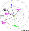 |
Fig. 1 Locations of planets in the inner Solar System on September 1, 2014 during the ejection of the CME E127. |
2 The 2014 September chain of events
A first fast halo CME was observed by Solar TErrestrial RElations Observatory – Behind (STEREO B) spacecraft on September 1, 2014 (Gopalswamy et al. 2020). The event had its origin in the solar active region 12158, as it is classified by the National Oceanic and Atmospheric Administration (NOAA), and located behind the east limb (N14E127) of the solar disk seen from the Earth (Plotnikov et al. 2017). Because of the relative proximity of Mercury, Earth, and Mars (see Fig. 1), this event affected the environments of the inner planets of the Solar System, inducing a strong enhancement both in proton and electron fluxes of solar origin, measured at Mercury and later on Mars and Earth. Due to the position of Mercury and STEREO B with respect to the direction of propagation of the September 1 CME, a sudden increase in the proton fluxes measured by STEREO B and the instrument Fast Imaging Plasma Spectrometer (FIPS) on board Mercury Surface, Space ENvironment, GEochemistry and Ranging (MESSENGER) can be seen in the upper panel of Fig. 2, while a gradual enhancement is observed at Mars and Earth from data obtained from the ion mass analyser (IMA) sensor of the Analyser of Space Plasma and Energetic Atoms (ASPERA-3) instrument on board Mars Express (MEX; Barabash et al. 2004), the High Energy Neutron Detector (HEND) on board Mars Odyssey (Zeitlin et al. 2010), and the Energetic and Relativistic Nuclei and Electron (ERNE) of the Solar and Heliospheric Observatory (SOHO) instruments, respectively. A second and then a third strong CME followed the one observed on September 1, occurring, respectively, on September 9 and 10, 2014. Both these CMEs originated from the same active region, 12158. This time, since the two CMEs propagated toward Earth and Mars, the enhancements in the proton fluxes are more evident and sharper for the particles measured at the Lagrange point 1 (L1) and at Mars, as can be seen from the lower panels of Fig. 2.
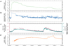 |
Fig. 2 Panel a: proton fluxes in the energy range within 10–20 MeVaa53169-24 measured by STEREO-B/LET from September 1– 15, 2014. Panel b: proton fluxes observed at Mercury by MESSEN- GER/FIPS instrument for the same date in the energy channel from 12.9 to 14 KeV (FIPS background counts in this energy channel can be caused by >1 MeV SEP electrons >10 MeV SEP protons; Gershman et al. 2015, 2016). Panel c: 15 keV 15 keV ion counts (which represent the background counts induced by SEP protons; Futaana et al. 2008) measured at Mars from September 1–15, 2014, by the IMA/ASPERA3 instrument on board Mars Express and HEND on Mars Odyssey in the energy range 195–>1000 keV (Sánchez–Cano et al. 2018). Panel d: proton fluxes measured by SOHO/ERNE instrument in the energy channel between 8 and 10 MeV, for the same time period. All the data plotted in panels a, b, and d were obtained from the AMDA database1. Data plotted in panel (c) were retrieved from NASA’s Planetary Data System web page2. |
3 Magnetic footpoint reconstruction
The intense fluxes of solar protons produced by the flares and the chain of CMEs occurred in the first half of September 2014 and traveled along the magnetic field lines of the solar wind, reaching the planetary bodies of the inner Solar System (Reames 2013). To better understand these processes, we applied a Monte Carlo (MC) simulation to study the interplanetary magnetic field lines transport in the solar wind (Ippolito et al. 2025, 2022, 2005). Such a simulation allowed us to reconstruct the magnetic footpoint of the Parker spiral connecting Mercury, the Earth, and Mars to the solar corona. In our model, the elementary displacement, dr, along the field line is parallel to B(r), since a magnetic field line is tangent by definition to the magnetic field at each point in space. This can be written as dr = Bdλ, where dλ is a scalar quantity. Choosing dλ as ds/|B|, the field line equations can be written as dr/ds = B/|B|, where ds is the arc length element along B. Besides, considering dλ as dξB0, with B0 constant and dξ a scalar quantity, one obtains
 (1)
(1)
where the magnetic field, B(r), is given by the average field,  , plus the fluctuation, δB(r).
To evaluate the quasi-linear magnetic field line diffusion coefficient in case of anisotropic turbulence, as observed in the solar wind, we considered a three-dimensional model of magnetic turbulence, represented as the sum of static magnetic perturbations (Pommois et al. 1999; Zimbardo et al. 2000):
![Mathematical equation: $\delta {\bf{B}}({\bf{r}}) = \sum\limits_{k,\sigma } \delta B({\bf{k}}){\widehat{\bf{e}}_\sigma }({\bf{k}})exp\,i\left[ {{\bf{k}}\cdot{\bf{r}} + {\phi _{\bf{k}}}^\sigma } \right],$](/articles/aa/full_html/2025/03/aa53169-24/aa53169-24-eq3.png) (2)
(2)
where  are the polarization unit vectors, while φkσ are random phases. The Fourier amplitude, δB(k), is represented by the spectrum:
 (3)
(3)
where γ = 3/2 represents the spectral index, and lx, ly, and lz are the correlation lengths in the x, y, and z directions, respectively. A random force term, proportional to the diffusion coefficient, was applied to the MC simulation, in addition to the magnetic field line equations. With this action, we can evaluate how the magnetic field lines diffuse with respect to the average field. A random displacement of the simulated field line was applied at each step of the integration along the Parker magnetic field model. To tailor to a specific event the reconstruction of the magnetic connection from a Solar System Body to the solar corona, the observed values of solar wind velocity and magnetic fluctuation level were ingested by the model,
 (4)
(4)
where i = x, y; ηx (ξ) and ηy (ξ) are two uncorrelated random functions, and  represents the random force amplitudes (Veltri et al. 1998; Ippolito et al. 2005).
The random displacement is proportional to a local diffusion coefficient that quantifies the local transport of magnetic field lines, considering the fluctuation level and the main features of the anisotropy of the solar wind turbulence (Pommois et al. 2001). We considered the z direction to be along the local average interplanetary magnetic field, B0 , the x direction to be normal to the plane formed by B0 and the radial direction (solar wind speed direction), and the y direction to complete the righthanded system. The average spiral field variation is much larger than the correlation length of the magnetic turbulence, so we computed the diffusion coefficients of magnetic field lines in a local frame in Cartesian geometry as follows:
 (5)
(5)
where D, μ, and ν are dimensionless parameters, and i = x,y. A best fit of the computed diffusion coefficient yields D = 0.028, μ = 1.51, and ν = 0.67 (Veltri et al. 1998; Zimbardo et al. 2000; Pommois et al. 2001). The turbulence correlation lengths in the x, y, and z directions, respectively, lx, ly, and lz, quantify the anisotropy of turbulence in the solar wind. From the literature, the typical fluctuation levels relevant to the solar wind are δB/B0 ≃ 0.5–1 (Zank et al. 1998). This corresponds to degrees of anisotropy of lx/1y = 1 ÷ 10 and 1z/1y = 1 ÷ 10.
The planets of the inner Solar System can be immersed in different plasma streams with a variable speed, at any given time. Since we do not know a priori the solar wind speed along the field lines that are magnetically connected to each planet, we used data from the Advanced Composition Explorer (ACE) satellite for the solar wind speed, considering 6 days before the occurrence of the considered event and computing the average velocity. When the average solar wind velocity is below 500 km/s, the uncertainty on the large-scale magnetic structure of the solar wind can be neglected. The position of the planets with respect to the current sheet represents further important information to determine whether each planet is surrounded by a positive or negative magnetic sector, which means a magnetic field outward or inward from the Sun (Russell 2001). To get such information, we considered the Source Surface Synoptic Charts produced by the Wilcox Solar Observatory (WSO). The WSO synoptic charts are produced by computing the photospheric field observations with a potential field model, forced to be radial at the source surface to approximate the effect of the accelerating solar wind on the field configuration (Hoeksema & Scherrer 1986). The resulting magnetic maps are based on the portion of the solar disk visible from the Earth, and show the strength, polarity, and location of the magnetic flux density at the solar source surface (r = 2.5 Rs). To describe the magnetic connection between the planets and the solar corona, we integrated Eq. (1) for approximately 105 field lines using the values of δB/B observed. Starting from the Earth’s magnetopause, from a circle with an estimated diameter of 40 RE (with RE being the Earth’s radius), we stopped the integration at r ≈ 3RS. We then plotted the distribution of field lines from the Earth to the arrival points at the solar wind source surface as contour levels. These represent the probability density of magnetic connection with the Earth, obtained from the numerical simulation, with isolevels spaced by a factor of 2. The positions of the magnetic field line are plotted in heliographic latitude and longitude, on the background of the magnetic field maps at the source surface of the solar wind, provided by the Wilcox Solar Observatory3. The position of the Earth, Mercury, and Mars, and their relative magnetic footpoints, together with the flare site (asterisk), have been projected on the solar magnetic configuration at the source surface. The thick solid line on the magnetogram represents the magnetic equator, while the thinner lines are the isointensity contours of |B|.
The results of the simulation, together with the additional information regarding the flares position and the magnetic configuration at source surface, are shown in Fig. 4. In this figure, we report the magnetic footpoints of the Earth (blue contour lines), Mars (green contour lines), and Mercury (petrol blue contour lines), traced back on the solar surface (4 solar radii) for September 1, 9, and 10, 2014, from top to bottom. Each panel also reports the projection of Earth (blue square), Mars (green square), and Mercury (petrol blue spot) and the flare sites. All these features are projected on the solar magnetic configuration provided by WSO at the source surface (r = 2.5 Rs).
4 SEP events: Particle fluxes at different locations (STEREO B, Mercury, Earth, and Mars)
The CME that occurred on September 1, 2014, led to an intense SEP event observed at Mercury, as can be clearly seen from the proton fluxes measured by FIPS/MESSENGER and reported in panel b of Fig. 2. From the upper panel of the same figure, it can be noticed how strong enhancements in the energetic proton fluxes have also been measured by the STEREO satellite due to its position with respect to the propagation direction of the CME shock (see Fig. 1). From the data taken by IMA/Mars Express and ERNE/SOHO, plotted, respectively, in panels c–e of Fig. 2, it can be seen how the increases in the energetic protons measured at L1 and at Mars are less evident and have a delay of some days. This is due to the fact that, because of their angular distance of Mars and the Earth from the propagation path of the CME, the associated shock wave, in its expansion in the interplanetary medium, takes a few days to reach the interplanetary magnetic field lines through which the accelerated protons can reach the two planets. The CME observed on September 9, 2014 most probably originated in a M4.5 flare in the eastern sector of the solar disk seen by the Earth. This CME, although not too fast and with a direction of propagation not favorable for being geo-effective, caused an evident enhancement in the energetic protons observed at Mars (see Fig. 2) starting on 10 September, since the shock wave associated with the CME was reasonably directed toward the planet. From Fig. 2, no appreciable increase is visible in the protons measured by FIPS/MESSENGER at Mercury, probably because the Hermian environment was still in a recovery phase from the stronger events triggered by the CME of September 1. Due to the higher angular distance with respect to the propagation direction of the shock, the enhancements in the proton fluxes observed at Earth are measured with more than a day of delay from the CME observation, starting from September 10. A further halo CME, reported by the STEREO and Wind WAVES type II bursts and the corresponding CMEs Catalog4 (Gopalswamy et al. 2018), associated with a X1.6 solar flare, was observed on September 10 coming from the same active region (AR12158) in which the September 1 and 9 CMEs originated. As can be deduced from the two lower panels of Fig. 3b, the X1.6 flare led to a fast CME that produced a gradual increase in the energetic pron fluxes measured by GOES satellite at L1. The peak of such an enhancement in the proton fluxes at Earth, also visible in Fig. 2, is delayed because of the angular distance of the AR origin of the CME with respect to the magnetic footpoint of the Parker spiral passing through our planet, as can be seen in the lower panel of Fig. 4. The proximity of the magnetic footpoint of Mercury to the site of the X-class flare that produced the CME would suggest that strong fluxes of energetic protons could have reached the planet. From the FIPS/MESSENGER measurements reported in Fig. 2, an enhancement can be seen in the observed particle at Mercury. Nevertheless, a lack of data, maybe due to the saturation of the instruments, prevents further consideration of the SEP event at Mercury. A gradual and smooth enhancement in the energetic proton fluxes has been also observed by STEREO B, and is visible in the data plotted in the upper panel of Fig. 2. From the IMA/MEX observations plotted in Fig. 2, an increase is clearly visible in the energetic protons in the Martian environment, due to the particles accelerated by the CME shock wave. The enhancement is quasi-simultaneous to the increase in the energetic particles measured at L1, because, though the radial distance from Mars to the Sun is greater, the magnetic footpoint of the Parker spiral passing through the planet, compared to the magnetic footpoint of the Earth, was at that time closer to the region of the solar corona in which the CME originated, as is described in the lower panel of Fig. 4.
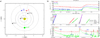 |
Fig. 3 Left panel: positions of the inner planets of the Solar System on September 10, 2014. Right panel: plots obtained from the STEREO and Wind WAVES type II bursts and the associated CMEs Catalog (Gopalswamy et al. 2018). The right panel reports the X-ray fluxes measured by the GOES satellite on September 10, 2014 (lower panel), together with the CME height-time plots (middle panel) and the energetic proton fluxes at L1 (upper panel). |
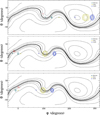 |
Fig. 4 From top to bottom: the magnetic footpoints of the Earth (blue contour lines), Mars (green contour lines), and Mercury (petrol blue contour lines), traced back on the solar surface (4 Solar radii) for September 1, 9, and 10, 2014, respectively. Each panel also reports the projection of Earth (blue square), Mars (green square), and Mercury (petrol blue spot) and of the flares site. All these features are projected on the solar magnetic configuration at the source surface (r = 2.5Rs) provided by WSO, in which the thick solid line represents the magnetic equator and the thinner lines the isointensity contours of |B|. |
5 Effects at Earth
Analyzing the geomagnetic disturbance Dst index (Mayaud 1980), which represents a 1-hour cadence proxy of the intensity of the axisymmetric currents flowing in the magnetosphere, including the ring current, the tail currents, and the magnetopause Chapman-Ferraro currents (Ganushkina et al. 2018), it can be seen from the lower panel of Fig. 5 how, starting on August 28, 2014, the geomagnetic field was characterized by a long recovery phase due to a previous geomagnetic storm recorded on August 26, 2014. The circumterrestrial environment was then strongly affected by a shock wave, probably the one related to the September 10 CME, which led to a further geomagnetic storm on September 12. This second storm reached a greater intensity than the previous one, as can be deduced from the peak value of the Dst index in Fig. 5, but lasted for a shorter interval of time since the Bz component of the IMF, plotted in the upper panel of Fig. 5, after a first negative phase that triggered the geomagnetic storm, suddenly started having positive values. An example of the disturbances produced by the September 12 geomagnetic storm (Ippolito et al. 2020) is the evident enhancement in the critical frequency of the ionospheric F2 layer recorded by the Rome ionospheric observatory. In addition, the flares that occurred on September 9 and 10, 2014, led to intense solar radio bursts observed at L1, as is demonstrated by the WIND/WAVES and STEREO-B/SWAVES instrument data for September 10, 2014, reported in Fig. 6.
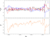 |
Fig. 5 Upper panel: values of the IMF components in the geocentric solar ecliptic coordinate system from August 26, 2014, to September 15, 2014. Lower panel: behavior of the geomagnetic disturbance Dst index from August 26, 2014, to September 15, 2014. |
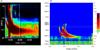 |
Fig. 6 Data from WIND/WAVES (left panel) and STEREO/SWAVES (right panel) for September 10, 2014. Clear signatures of solar radio bursts can be seen from both instruments. |
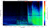 |
Fig. 7 Chain of type III solar radio bursts detected by Mars Express MARSIS-AIS instrument on September 10, 2014. The arrival time of the solar radio bursts is indicated with a vertical dashed red line. The horizontal yellow-green lines below 1.5 MHz at the center of the figure correspond to ionospheric reflections as MARSIS is a radar designed to sound the ionosphere of Mars. |
6 Impact on the Martian environment
Type III solar radio bursts tend to occur after the ejection of powerful CMEs and solar flares, drifting rapidly from high to low frequencies. These emissions can also be observed by MAR- SIS/MEX in the range frequency 0.1–5.5 MHz if they occur during the window of operation of the radar in its Active Ionospheric Sounding mode (Sanchez-Cano et al., under review). During the events studied here, three solar radio bursts were observed on September 10, 2014. Their arrival times concatenate, as can be seen in Fig. 7, and match pretty well with the solar radio bursts observed by STEREO-B in Fig. 6 in time and intensity. Other features from the ionosphere of the planet are also seen in the MARSIS data shown in Fig. 7 (see Sanchez-Cano et al., (under review) for a comprehensive review of them). Here, we analyze MARSIS surface and ionospheric echoes to characterize the Martian ionospheric response to this space weather event. Figure 8 shows the overview of the MEX observations from August 26 to September 25, 2014. To provide the space weather context, Fig. 8a shows 10-min averaged background counts of IMA in the highest-energy channel as a proxy of the SEP flux. We observe two distinct enhancements of the IMA background level corresponding to the SEP events, as is discussed in Sect. 2. Coinciding with these SEP proxy enhancements, the surface echo power at 5–5.5 MHz recorded by MARSIS is significantly reduced (Fig. 8b). This indicates that the transmitted radio pulse is substantially attenuated by electron–neutral collisions in the lower ionosphere of Mars as a result of enhanced ionization by energetic particle precipitation. Notably, we observe prolonged radio absorption perhaps with a small recovery on September 10, 2014 (Fig. 8b), even though the SEP proxy from IMA shows two distinct peaks (Fig. 8a).
Figure 8c shows the range spread of 1.4–1.6 MHz ionospheric echoes measured by MARSIS. Here, the range spread is represented by the number of range bins with an echo power exceeding 10−15 (V∕m)2 ∕Hz in an apparent altitude range of 50–200 km. The diamonds and error bars in Fig. 8c show the average and standard deviation of this range spread indicator for each periapsis leg of MARSIS observations, respectively. The ionospheric echoes with a range spread, also known as diffuse echoes, are thought to result from ionospheric irregularities (Gurnett et al. 2008; Harada et al. 2018b). Morgan et al. (2014) reported that many diffuse ionospheric echoes were detected by MARSIS during an ICME passage in 2011, implying the formation of complex structures of the topside ionosphere of Mars during space weather events. During the September 2014 event, we identify two orbits with particularly prominent diffuse echoes, orbits 13549 and 13595. Radargrams from these two orbits are shown in Figs. 8f and 8g. We observe the diffuse nature of the ionospheric echoes for most of the time intervals of the two orbits. We note that MARSIS conducted topside sounding over the equatorial and northern regions in these orbits (Fig. 8e), and the diffuse echoes are not necessarily associated with strong crustal magnetic field regions. As opposed to the prolonged radio absorption (Fig. 8b), the ionospheric echoes with an enhanced range spread occur only sporadically (Fig. 8c). This suggests that the formation of ionospheric irregularities is spatially localized, temporally limited, or both, perhaps resulting from the dynamic solar wind interaction with the upper atmosphere of Mars during the space weather event.
 |
Fig. 8 Overview of MEX observations of the Martian ionospheric response to the September 2014 space weather event. Time series data of (a) 10-min averaged counts of Mars Express IMA in the highest energy channel representing the background level, which can be used as a proxy for SEP protons (Futaana et al. 2008), (b) 5–5.5 MHz surface echo power measured by MARSIS, the reduction of which indicates radio absorption in the lower ionosphere of Mars, derived in the same manner as (Harada et al. 2023), (c) range spread of 1.4–1.6 MHz ionospheric echoes derived from periapsis MARSIS observations, showing the level of ionospheric irregularities in the topside ionosphere of Mars (Harada et al. 2018a), and (d) solar zenith angle of Mars Express. Panel e: geographic map of periapsis MARSIS observations, with colors indicating the range spread of 1.4–1.6 MHz ionospheric echoes. Radargrams demonstrate the range spread of 1.4–1.6 MHz ionospheric echoes for orbits (f) 13549 and (g) 13595. |
7 Summary and conclusions
In this study, we provide an overview of some of the effects of a series of CMEs that occurred on September 1, 9, and 10, 2014, on the planetary environments of the inner Solar System. All these solar events originated in the same active region (AR12158). To better understand the propagation of SEPs and their impact on the different planetary environments, we studied the magnetic connection from the inner planets of the Solar System to the solar corona, in relation to the three CME events. Using a MC simulation with a test particle approach, we reconstructed the magnetic footpoints of the Parker spiral passing through Mercury, Mars, and Earth.
The halo CME on September 1, directed toward Mercury and STEREO B, resulted in a significant increase in proton fluxes measured by the MESSENGER and STEREO B spacecraft. In contrast, a gradual enhancement in proton fluxes was observed at Earth and Mars, as is reported by SOHO and MESSENGER, respectively. Analyzing the footpoints of the Parker spiral on the Solar surface, we found that the large angular distance from the CME source (indicated by the red asterisk in the top panel of Fig. 4) for Mars and Earth explains the delayed arrival of energetic particles accelerated by the CME’s shock wave. This resulted in a gradual and less intense increase in proton fluxes, as is illustrated in panels c and d of Fig. 2. Additionally, diffusive ionospheric echoes were detected in the MARSIS/AIS ionograms, likely due to electron density irregularities in the Martian ionosphere caused by the space weather event. A second CME, likely associated with an M4.5 flare, caused a noticeable increase in solar protons at Mars, occurring several hours before a rise in 10 MeV proton fluxes measured at L1 by SOHO. Given the projection of Mars’s position on the solar surface, indicated by the green circle in the middle panel of Fig. 4, it was much closer to the flare site (less than 20° in heliographic longitude, while the projection of the Earth (blue box) lies at more than 90° in heliographic longitude), and is thus more directly exposed to the CME’s propagation, the energetic particles accelerated by the associated shock wave reached the region in interplanetary space linked by IMF field lines to Mars well ahead of the portion of space where magnetic connections between Earth and the Solar corona became favorable. Despite the substantial increase in solar protons observed at L1, no geomagnetic disturbances were triggered by this CME due to the positive phase of the IMF Bz component. The third CME we analyzed, which occurred on September 10, 2014, was related to an X1.6 flare. Type II and type III solar radio bursts were detected by both WIND/WAVES and STEREO/SWAVES instruments, in association with the X- class flare (see Fig. 6). Due to the relatively high angular distance (more than 110° in Heliographic longitude) between the flare site, which is most probably the source of the CME, and the Earth’s magnetic footpoint, represented by the blue contour lines in the lower panel of Fig. 4, the energetic protons accelerated in this event reached the Earth only on September 11. Nevertheless the CME associated shock wave hit the Earth on September 12, causing a moderate geomagnetic storm, aided by the negative phase of the IMF Bz component (see 5). An enhancement in the energetic particles measured at Mars is clearly visible almost at the same time as a sudden increase in the proton fluxes is observed at L1 (see panels c and d of Fig. 2). This is because, although the radial distance from the Sun is higher, the magnetic footpoint of the Parker spiral passing through Mars appears to be closer (less than 100° in Heliographic longitude) to the flare site than the Earth’s footpoint, so the CME shock wave first reached the region in space where magnetic field lines connecting Mars to the solar corona are located. The effects of this intense solar emission are also captured in the MARSIS/AIS data, as is shown in Fig. 7. The diffusion observed in the MARSIS/AIS ionograms on September 16, 2014, depicted in panel g) of Fig. 8, likely corresponds to a CME that occurred on September 14. The goal of this work is to provide a comprehensive understanding of the potential effects of strong space weather events on the planetary environments of the inner Solar System. The multispacecraft and multi-parameter analysis presented here, along with the numerical simulations reconstructing the magnetic footpoints of the Parker spiral on the Sun’s surface, offer a detailed cause-and-effect framework for studying space weather events in the Solar System, allowing us to obtain a more global picture of the related phenomenon in action.
Acknowledgements
B.S.-C. acknowledges support through UK-STFC Ernest Rutherford Fellowship ST/V004115/1. Y.H. acknowledges support through JSPS KAKENHI Grant (22K14085, 22H01285,22KK0045).
References
- Barabash, S., Lundin, R., Andersson, H., et al. 2004, Mars Express: the Scientific Payload, 1240, 121 [NASA ADS] [Google Scholar]
- Campbell, B. A., Morgan, G. A., & Sánchez-Cano, B. 2024, Geophys. Res. Lett., 51, e2023GL105758 [Google Scholar]
- Cartacci, M., Amata, E., Cicchetti, A., et al. 2013, Icarus, 223, 423 [NASA ADS] [CrossRef] [Google Scholar]
- Cartacci, M., Sánchez-Cano, B., Orosei, R., et al. 2018, Icarus, 299, 396 [NASA ADS] [CrossRef] [Google Scholar]
- Futaana, Y., Barabash, S., Yamauchi, M., et al. 2008, Planet. Space Sci., 56, 873 [Google Scholar]
- Ganushkina, N. Y., Liemohn, M. W., & Dubyagin, S. 2018, Rev. Geophys., 56, 309 [NASA ADS] [CrossRef] [Google Scholar]
- Gershman, D. J., Raines, J. M., Slavin, J. A., et al. 2015, J. Geophys. Res. Space Phys., 120, 8559 [Google Scholar]
- Gershman, D. J., Dorelli, J. C., DiBraccio, G. A., et al. 2016, Geophys. Res. Lett., 43, 5935 [Google Scholar]
- Gopalswamy, N., Mäkelä, P., Yashiro, S., et al. 2018, ApJ, 868, L19 [NASA ADS] [CrossRef] [Google Scholar]
- Gopalswamy, N., Mäkelä, P., Yashiro, S., et al. 2020, Sol. Phys., 295, 18 [NASA ADS] [CrossRef] [Google Scholar]
- Gurnett, D., Huff, R., Morgan, D., et al. 2008, Adv. Space Res., 41, 1335 [Google Scholar]
- Harada, Y., Gurnett, D. A., Kopf, A. J., Halekas, J. S., & Ruhunusiri, S. 2018a, J. Geophys. Res.: Space Phys., 123, 1018 [Google Scholar]
- Harada, Y., Gurnett, D. A., Kopf, A. J., et al. 2018b, Geophys. Res. Lett., 45, 7960 [Google Scholar]
- Harada, Y., Nakamura, Y., Sánchez-Cano, B., et al. 2023, Space Weather, 21, e2023SW003755 [Google Scholar]
- Harada, Y., Fujiwara, Y., Lillis, R. J., 2024, Earth Planets Space, 76, 1880 [Google Scholar]
- Harada, Y., Sánchez-Cano, B., Lester, M., & Ippolito, A. 2025, Icarus, 425, 116342 [NASA ADS] [CrossRef] [Google Scholar]
- Herbst, K., Banjac, S., Atri, D., & Nordheim, T. A. 2020, A&A, 633, A15 [NASA ADS] [CrossRef] [EDP Sciences] [Google Scholar]
- Hoeksema, J., & Scherrer, P. H. 1986, Sol. Phys., 105, 205 [Google Scholar]
- Ippolito, A., Pommois, P., Zimbardo, G., & Veltri, P. 2005, A&A, 438, 705 [NASA ADS] [CrossRef] [EDP Sciences] [Google Scholar]
- Ippolito, A., Perrone, L., Plainaki, C., & Cesaroni, C. 2020, J. Space Weather Space Clim., 10, 52 [NASA ADS] [Google Scholar]
- Ippolito, A., Plainaki, C., Zimbardo, G., et al. 2022, A&A, 660, A50 [NASA ADS] [CrossRef] [EDP Sciences] [Google Scholar]
- Ippolito, A., Alberti, T., & Giannattasio, F. 2025, ApJ, 979, 146 [NASA ADS] [Google Scholar]
- Kajdic, P., Sánchez-Cano, B., Neves-Ribeiro, L., et al. 2021, J. Geophys. Res.: Space Phys., 126, e2020JA028442 [Google Scholar]
- Khoo, L. Y., Sánchez-Cano, B., Lee, C. O., et al. 2024, ApJ, 963, 107 [NASA ADS] [CrossRef] [Google Scholar]
- Leblanc, F., Luhmann, J. G., Johnson, R. E., & Liu, M. 2003, Planet. Space Sci., 51, 339 [NASA ADS] [CrossRef] [Google Scholar]
- Lester, M., Sanchez-Cano, B., Potts, D., et al. 2022, J. Geophys. Res.: Space Phys., 127, e2021JA029535 [Google Scholar]
- Lilensten, J., Coates, A. J., Dehant, V., et al. 2014, A&ARv,, 22, 79 [Google Scholar]
- Lillis, R. J., Deighan, J., Brain, D., et al. 2022, Geophys. Res. Lett., 49, e2022GL099820 [Google Scholar]
- Mayaud, P. N. 1980, Geophys. Monogr. Ser., 22 [Google Scholar]
- Milillo, A., Mangano, V., Massetti, S., et al. 2021, Icarus, 355, 114 [Google Scholar]
- Morgan, D. D., Diéval, C., Gurnett, D. A., et al. 2014, J. Geophys. Res.: Space Phys., 119, 5891 [Google Scholar]
- Nordheim, T., Dartnell, L., Desorgher, L., Coates, A., & Jonesi, G. 2015, Icarus, 245, 80 [NASA ADS] [CrossRef] [Google Scholar]
- Orsini, S., Milillo, A., Lichtenegger, H., et al. 2022, Nat. Commun., 13, 7390 [Google Scholar]
- Orsini, S., Mangano, V., Milillo, A., et al. 2024, Sci. Rep., 14, 30728 [Google Scholar]
- Palmerio, E., Kilpua, E. K. J., Witasse, O., et al. 2021, Space Weather, 19, e2020SW002654 [NASA ADS] [CrossRef] [Google Scholar]
- Plainaki, C., Lilensten, J., Radioti, A., et al. 2016a, J. Space Weather Space Clim., 6, A31 [NASA ADS] [CrossRef] [EDP Sciences] [Google Scholar]
- Plainaki, C., Paschalis, P., Grassi, D., Mavromichalaki, H., & Andriopoulou, M. 2016b, Ann. Geophys., 34, 595 [NASA ADS] [Google Scholar]
- Plotnikov, I., Rouillard, A. P., & Share, G. H. 2017, A&A, 608, A43 [NASA ADS] [CrossRef] [EDP Sciences] [Google Scholar]
- Pommois, P., Veltri, P., & Zimbardo, G. 1999, Phys. Rev. E, 59, 2244 [Google Scholar]
- Pommois, P., Veltri, P., & Zimbardo, G. 2001, J. Geophys. Res.: Space Phys., 106, 24965 [NASA ADS] [CrossRef] [Google Scholar]
- Reames, D. V. 2013, Space Sci. Rev., 1275, 53 [Google Scholar]
- Russell, C. T. 2001, Geophys. Monogr.-Am. Geophys. Union, 125, 73 [Google Scholar]
- Sánchez-Cano, B., Hall, B. E. S., Lester, M., et al. 2017, J. Geophys. Res.: Space Phys., 122, 6611 [Google Scholar]
- Sánchez–Cano, B., Witasse, O., Lester, M., et al. 2018, J. Geophys. Res.: Space Phys., 123, 8778 [Google Scholar]
- Sánchez–Cano, B., Blelly, P. L., Lester, M., et al. 2019, J. Geophys. Res.: Space Phys., 124, 4556 [Google Scholar]
- Sánchez–Cano, B., Lester, M., Andrews, D. J., et al. 2021, Exp. Astron., 54, 641 [Google Scholar]
- Schneider, N. M., Milby, Z., Jain, S. K., et al. 2021, J. Geophys. Res.: Space Phys., 126, e2021JA029428 [Google Scholar]
- Tobias, S., Brummell, N. H., Clune, T. L., & Toomre, J. 2001, ApJ, 549, 1183 [NASA ADS] [CrossRef] [Google Scholar]
- Tripathi, K. R., Imamura, T., Choudhary, R. K., Sánchez–Cano, B., & Ambili, K. M. 2024, Geophys. Res. Lett., 51, e2024GL109724 [Google Scholar]
- Veltri, P., Zimbardo, G., & Pommois, P. 1998, Adv. Space Res., 22, 55 [NASA ADS] [CrossRef] [Google Scholar]
- Winslow, R. M., Lugaz, N., Philpott, L. C., et al. 2015, J. Geophys. Res.: Space Phys., 120, 1601 [Google Scholar]
- Witasse, O., Sánchez-Cano, B., Mays, M. L., et al. 2017, JGR Space Phys., 122, 7865 [Google Scholar]
- Withers, P., Felici, M., Mendillo, M., et al. 2022, J. Geophys. Res.: Space Phys., 127, e2022JA030737 [Google Scholar]
- Xu, S., Weber, T., Mitchell, D. L., et al. 2019, J. Geophys. Res.: Space Phys., 124, 1823 [Google Scholar]
- Yu, B., Chi, Y., Owens, M., et al. 2023, ApJ, 953, 105 [NASA ADS] [Google Scholar]
- Zank, G. P., Matthaeus, W. H., Bieber, J. W., & H., M. 1998, J. Geophys. Res.: Space Phys., 103, 2085 [NASA ADS] [CrossRef] [Google Scholar]
- Zeitlin, C., Boynton, W., Mitrofanov, I., et al. 2010, Space Weather, 8, https://agupubs.onlinelibrary.wiley.com/doi/pdf/10.1029/2009SW000563 [Google Scholar]
- Zimbardo, G., Veltri, P., & Pommois, P. 2000, Phys. Rev. E, 61, 1940 [NASA ADS] [CrossRef] [Google Scholar]
All Figures
|
Fig. 1 Locations of planets in the inner Solar System on September 1, 2014 during the ejection of the CME E127. |
| In the text | |
|
Fig. 2 Panel a: proton fluxes in the energy range within 10–20 MeVaa53169-24 measured by STEREO-B/LET from September 1– 15, 2014. Panel b: proton fluxes observed at Mercury by MESSEN- GER/FIPS instrument for the same date in the energy channel from 12.9 to 14 KeV (FIPS background counts in this energy channel can be caused by >1 MeV SEP electrons >10 MeV SEP protons; Gershman et al. 2015, 2016). Panel c: 15 keV 15 keV ion counts (which represent the background counts induced by SEP protons; Futaana et al. 2008) measured at Mars from September 1–15, 2014, by the IMA/ASPERA3 instrument on board Mars Express and HEND on Mars Odyssey in the energy range 195–>1000 keV (Sánchez–Cano et al. 2018). Panel d: proton fluxes measured by SOHO/ERNE instrument in the energy channel between 8 and 10 MeV, for the same time period. All the data plotted in panels a, b, and d were obtained from the AMDA database1. Data plotted in panel (c) were retrieved from NASA’s Planetary Data System web page2. |
| In the text | |
|
Fig. 3 Left panel: positions of the inner planets of the Solar System on September 10, 2014. Right panel: plots obtained from the STEREO and Wind WAVES type II bursts and the associated CMEs Catalog (Gopalswamy et al. 2018). The right panel reports the X-ray fluxes measured by the GOES satellite on September 10, 2014 (lower panel), together with the CME height-time plots (middle panel) and the energetic proton fluxes at L1 (upper panel). |
| In the text | |
|
Fig. 4 From top to bottom: the magnetic footpoints of the Earth (blue contour lines), Mars (green contour lines), and Mercury (petrol blue contour lines), traced back on the solar surface (4 Solar radii) for September 1, 9, and 10, 2014, respectively. Each panel also reports the projection of Earth (blue square), Mars (green square), and Mercury (petrol blue spot) and of the flares site. All these features are projected on the solar magnetic configuration at the source surface (r = 2.5Rs) provided by WSO, in which the thick solid line represents the magnetic equator and the thinner lines the isointensity contours of |B|. |
| In the text | |
|
Fig. 5 Upper panel: values of the IMF components in the geocentric solar ecliptic coordinate system from August 26, 2014, to September 15, 2014. Lower panel: behavior of the geomagnetic disturbance Dst index from August 26, 2014, to September 15, 2014. |
| In the text | |
|
Fig. 6 Data from WIND/WAVES (left panel) and STEREO/SWAVES (right panel) for September 10, 2014. Clear signatures of solar radio bursts can be seen from both instruments. |
| In the text | |
|
Fig. 7 Chain of type III solar radio bursts detected by Mars Express MARSIS-AIS instrument on September 10, 2014. The arrival time of the solar radio bursts is indicated with a vertical dashed red line. The horizontal yellow-green lines below 1.5 MHz at the center of the figure correspond to ionospheric reflections as MARSIS is a radar designed to sound the ionosphere of Mars. |
| In the text | |
|
Fig. 8 Overview of MEX observations of the Martian ionospheric response to the September 2014 space weather event. Time series data of (a) 10-min averaged counts of Mars Express IMA in the highest energy channel representing the background level, which can be used as a proxy for SEP protons (Futaana et al. 2008), (b) 5–5.5 MHz surface echo power measured by MARSIS, the reduction of which indicates radio absorption in the lower ionosphere of Mars, derived in the same manner as (Harada et al. 2023), (c) range spread of 1.4–1.6 MHz ionospheric echoes derived from periapsis MARSIS observations, showing the level of ionospheric irregularities in the topside ionosphere of Mars (Harada et al. 2018a), and (d) solar zenith angle of Mars Express. Panel e: geographic map of periapsis MARSIS observations, with colors indicating the range spread of 1.4–1.6 MHz ionospheric echoes. Radargrams demonstrate the range spread of 1.4–1.6 MHz ionospheric echoes for orbits (f) 13549 and (g) 13595. |
| In the text | |
Current usage metrics show cumulative count of Article Views (full-text article views including HTML views, PDF and ePub downloads, according to the available data) and Abstracts Views on Vision4Press platform.
Data correspond to usage on the plateform after 2015. The current usage metrics is available 48-96 hours after online publication and is updated daily on week days.
Initial download of the metrics may take a while.