| Issue |
A&A
Volume 689, September 2024
|
|
|---|---|---|
| Article Number | A247 | |
| Number of page(s) | 21 | |
| Section | Extragalactic astronomy | |
| DOI | https://doi.org/10.1051/0004-6361/202449194 | |
| Published online | 17 September 2024 | |
The XMM-Newton and NuSTAR view of IRASF11119+3257
I. Detection of multiple ultra fast outflow components and a very cold corona
1
INAF – Osservatorio di Astrofisica e Scienza dello Spazio di Bologna, Via Gobetti, 93/3, 40129 Bologna, Italy
2
Department of Physics and Astronomy (DIFA), University of Bologna, Via Gobetti, 93/2, 40129 Bologna, Italy
3
Quasar Science Resources SL for ESA, European Space Astronomy Centre (ESAC), Science Operations Department, 28692 Villanueva de la Cañada, Madrid, Spain
4
Max Planck Institute für Extraterrestriche Physik, Giessenbachstrasse, 85748 Garching, Germany
5
INAF – Osservatorio Astrofisico di Arcetri, Largo Enrico Fermi 5, 50125 Firenze, Italy
6
Department of Physics, University of Rome ‘Tor Vergata’, Via della Ricerca Scientifica 1, 00133 Rome, Italy
7
INAF – Osservatorio Astronomico di Roma, Via Frascati 33, 00078 Monte Porzio Catone, (Roma), Italy
8
INFN – Rome Tor Vergata, Via della Ricerca Scientifica 1, 00133 Rome, Italy
9
Department of Astronomy, University of Maryland, College Park, MD 20742, USA
10
NASA Goddard Space Flight Center, Code 662, Greenbelt, MD 20771, USA
11
INAF – Istituto di Astrofisica e Planetologia Spaziali, Via Fosso del Cavaliere, 00133 Roma, Italy
12
Department of Physics, Institute for Astrophysics and Computational Sciences, The Catholic University of America, Washington, DC 20064, USA
13
INAF – Osservatorio Astronomico di Brera, Via Bianchi 46, 23807 Merate, LC, Italy
14
Dipartimento di Fisica, Universitá di Trento, Via Sommarive 14, Trento 38123, Italy
15
Department of Physics and Astronomy, College of Charleston, Charleston, SC 29424, USA
16
Dipartimento di Matematica e Fisica, Università degli Studi Roma Tre, Via della Vasca Navale 84, 00146 Roma, Italy
17
Department of Physics, Informatics and Mathematics, University of Modena and Reggio Emilia, 41125 Modena, Italy
18
Centro de Astrobiologia (CAB), CSIC-INTA, Departamento de Astrofisica, Cra. de Ajalvir Km. 4, 28850 Torrejon de Ardoz, Madrid, Spain
19
Joint Space-Science Institute, University of Maryland, College Park, MD 20742, USA
Received:
9
January
2024
Accepted:
17
June
2024
Context. IRASF11119+3257 is an ultra-luminous infrared galaxy with a post-merger morphology, hosting a type-1 quasar at z = 0.189. It shows a prominent ultra-fast outflow (UFO) absorption feature (vout ∼ 0.25c) in its 2013 Suzaku spectrum. This is the first system in which the energy released by the UFO was compared to that of the known galaxy-scale molecular outflow to investigate the mechanism driving active galactic nuclei (AGN) feedback.
Aims. In 2021, we obtained the first XMM-Newton long look of the target, coordinated with a simultaneous NuSTAR observation, with the goal of constraining the broad band continuum and the nuclear wind physical properties and energetics with an unprecedented accuracy.
Methods. The new high-quality data allowed us to clearly detect at a confidence level P > 99.8% multiple absorption features associated with the known UFO at the 9.1 and 11.0 keV rest frames. Furthermore, an emission plus absorption feature at 1.1 − 1.3 keV reveals the presence of a blueshifted P-Cygni profile in the soft band.
Results. We associate the two hard band features with blends of FeXXV and FeXXVI Heα-Lyα and Heβ-Lyβ line pairs and infer a large column (NH ∼ 1024 cm−2) of highly ionized (log ξ ∼ 5) gas outflowing at vout = 0.27 ± 0.01c. The 1.3 keV absorption line can be associated with a blend of Fe and Ne transitions, produced by a lower column (NH ∼ 3 × 1021 cm−2) and ionization (log ξ ∼ 2.6) gas component outflowing at the same speed. Using a radiative-transfer disk wind model to fit the highly ionized UFO, we derive a mass outflow rate comparable with the mass accretion rate and the Eddington limit (Ṁout = 4.25−0.73+1.11 M⊙/yr, ∼1.6 Ṁacc and ∼1.0 ṀEdd), and kinetic energy (Ėkin = 1.21−0.20+0.32 Lbol and ∼0.7LEdd) and momentum flux (Ṗout = 6.37−1.09+1.67 Lbol/c) among the highest reported in the literature. We measured an extremely low high-energy cutoff (Ecut ∼ 25 − 30 keV). This and several other cases in the literature suggest that a steep X-ray continuum may be related to the formation of powerful winds. We also analyzed the ionized [OIII] component of the large-scale outflow through optical spectroscopy and derived a large outflow velocity (vout ∼ 3000 km/s) and energetics comparable with the large-scale molecular outflows. Finally, we observe a trend of decreasing outflow velocity from forbidden optical emission lines of decreasing ionization levels, interpreted as the outflow decelerating at large distances from the ionizing source.
Conclusions. The lack of a significant momentum boost between the nuclear UFO and the different phases of the large-scale outflow, observed in IRASF11119 and in a growing number of similar sources, can be explained by (i) a momentum-driven expansion, (ii) an inefficient coupling of the UFO with the host interstellar medium, or (iii) by repeated energy-driven expansion episodes with a low duty cycle, that average out on long timescales to produce the observed large-scale outflow.
Key words: galaxies: active / galaxies: nuclei / quasars: absorption lines / quasars: supermassive black holes / quasars: individual: IRAS F11119+3257
© The Authors 2024
 Open Access article, published by EDP Sciences, under the terms of the Creative Commons Attribution License (https://creativecommons.org/licenses/by/4.0), which permits unrestricted use, distribution, and reproduction in any medium, provided the original work is properly cited.
This article is published in open access under the Subscribe to Open model. Subscribe to A&A to support open access publication.
1. Introduction
Ultra fast outflows (UFOs, vout > 104 km s−1) launched in the vicinity of accreting super massive black holes (SMBH) were first discovered in the luminous lensed quasars APM 08279+5255 (Hasinger et al. 2002; Chartas et al. 2002) and in two low-redshift analogs, PG 1211+143 (Pounds et al. 2003) and PDS 456 (Reeves et al. 2003). They are now routinely detected as blue-shifted iron K-shell absorption lines at energies above ∼7 keV in the X-ray spectra of 30–40% of low redshift (z < 0.5) Seyferts (Tombesi et al. 2010; Gofford et al. 2013), quasars (Matzeu et al. 2023), and radio galaxies (Tombesi et al. 2014) and in an even larger fraction of the few – mostly lensed – high redshift (i.e., z ≳ 2) quasars with good enough X-ray spectra (Bertola et al. 2020; Chartas et al. 2021).
These nuclear winds span a wide range in velocity (from the defining threshold of vout > 104 km s−1, up to ∼0.3 − 0.5c, e.g., Reeves et al. 2018a; Chartas et al. 2009), with gas column densities and ionization parameters in the ranges log(NH/cm−2) ∼ 23 − 24 and log(ξ/erg cm s−1) ∼ 3 − 6, respectively. Given their physical properties and their likely wide-angle geometry nature – consistently derived from both the detection rate in the general active galactic nuclei (AGN) population and the observed P-Cygni profile shape in a few well-studied examples (e.g., Nardini et al. 2015; Laurenti et al. 2021) – they are expected to deposit a significant fraction of the SMBH accretion power into the host galaxy (e.g., Gaspari et al. 2012).
Warm absorbers (WA) with much lower column densities (log(NH/cm−2) ∼ 20 − 22) and ionization parameters (log(ξ/erg cm s−1) ∼ 1 − 3) are observed as absorption features and edges from He- and H-like ions of C, O, N, Ne, Mg, and other elements mostly in the soft X-ray band (e.g., Blustin et al. 2005). These outflows have a much lower velocity (up to 5 × 10³ km/s), and even if they are detected in an even larger fraction of AGN, that is, ∼65% (Reynolds 1997; Piconcelli et al. 2005; McKernan et al. 2007), they are estimated to carry only a small fraction of the kinetic energy of the outflow.
The claim of high-velocity ionized outflow detected in the soft band dates back to the very beginning of the nuclear wind studies era (Pounds et al. 2003) and has been recently reported in a growing number of local Seyferts and quasars (Gupta et al. 2013b, 2015; Longinotti et al. 2015; Reeves et al. 2016, 2018b; Pounds et al. 2016; Parker et al. 2017; Serafinelli et al. 2019; Krongold et al. 2021).
These absorbers, often observed in high-resolution grating spectra in the soft X-ray band, are attributed to gas clouds with a much lower ionization and column densities with respect to UFOs but with comparable outflow velocities. This class of outflows can be interpreted as being due to dense clumps of shocked interstellar medium entrained at large distances (hundreds of parsecs) by the advancing outer shock (Faucher-Giguère & Quataert 2012; Zubovas & King 2012), or as the imprint of the UFO gas itself cooling down and fragmenting at hundreds of Rg from the SMBH (Takeuchi et al. 2013; Kobayashi et al. 2018; Gaspari & Sądowski 2017). In both cases, Rayleigh-Taylor and Kelvin-Helmholtz’s instabilities are central to the process, as well as turbulence and radiative multiphase condensation, for example, via chaotic cold accretion (CCA) mechanism (Gaspari et al. 2017).
All these multiphase and multiscale winds driven by the central AGN are thought to play a fundamental role in shaping the SMBH/galaxy coevolution (e.g., Fabian 2012; Gaspari et al. 2020; Veilleux et al. 2020; Laha et al. 2021) by removing and/or heating the cold gas from the host, quenching the growth of both the SMBH and the stellar component – the so-called AGN feedback – and possibly driving the scaling relations between the SMBH mass and host properties (e.g., Silk & Rees 1998; Magorrian et al. 1998).
Finding observational evidence for AGN feedback in action is of crucial importance to understanding galaxy and SMBH evolution (e.g., Fiore et al. 2017). Theoretical models suggest energy- or momentum-conserving flows powered by the nuclear UFO (e.g., Zubovas & King 2012; Costa et al. 2014) as the driving mechanism of the large-scale outflows. Momentum-conserving flows occur if most of the wind kinetic energy is radiated away. Energy-conserving flows occur if the gas that is shock heated by the wind is not efficiently cooled and instead expands adiabatically as a hot bubble. In the latter case, the momentum rate of the large-scale outflow is boosted by a factor ∝vdw/vls, where vdw is the velocity of the nuclear disk wind and vls the velocity of the large-scale outflow.
Originally, studies of large-scale molecular outflows lacked the detection of the inner winds (e.g., Veilleux et al. 2013). Conversely, studies of AGN accretion disk winds focused only on X-ray observations of local AGNs (e.g., Tombesi et al. 2010; Gofford et al. 2013) and a few high redshift quasars (Chartas et al. 2002; Lanzuisi et al. 2012; Bertola et al. 2020). This situation changed when the detection of an accretion disk wind and a powerful molecular outflow was reported in the same source, IRAS F11119+3257 (IRAS F11119 hereafter; Tombesi et al. 2015, hereafter T15), finding momentum flux values supporting the energy-driven scenario. Later studies (Veilleux et al. 2017) revised the energetics of the large-scale outflow – also seen in CO(1–0) emission line wings with ALMA – by time-averaging over the flow time and adopted different assumptions on the covering factor and coupling of the UFO with the ISM, obtaining energetics for the wind more in line with the momentum-driven scenario (see also Nardini & Zubovas 2018 who also revised the BH mass).
These results started an entirely new line of research trying to observationally link the small-scale relativistic winds and the large-scale outflows in a few bright local and high-z AGNs (e.g., Feruglio et al. 2017; Chartas et al. 2020) through the use of the “momentum boost” diagram and similar metrics (e.g., the energy-transfer rate). The observational evidence, however, has shown contradictory results, with different systems showing a variety of behaviors in terms of outflow energetics (e.g., Reeves & Braito 2019; Smith et al. 2019; Bischetti et al. 2019; Marasco et al. 2020; Tozzi et al. 2021). Because of the large uncertainties affecting these measurements and the limited samples (see, e.g., Bonanomi et al. 2023 for a recent compilation) up to now, the results are inconclusive. Variability on different time scales is an unavoidable complication in these studies, as both the nuclear wind power and the SMBH accretion rate vary on time scales that are much shorter than the galaxy-scale winds flow time (see, e.g., Zubovas & Nardini 2020).
In this paper, we analyze new XMM-Newton and NuSTAR data of IRASF11119 to derive accurate physical parameters and energetics for the persistent nuclear outflow observed in X-rays and test the energy-driving scenario for the impact of such outflow on large scales. The paper is organized as follows: Sect. 2 illustrates the target properties; Sect. 3 describes the procedures adopted in data reduction; in Sect. 4 we describe the continuum modeling and the search for absorption and emission features; in Sect. 5 we derive the main properties and statistical significance of the detected features, while in Sect. 6 we model the UFO features with physical wind models; in Sect. 7, we discuss the possible connection between outflows and coronal properties; in Sect. 8, we derive the properties of the large-scale ionized outflow from optical spectroscopy; in Sect. 9, we derive the energetics of the nuclear and large-scale ionized outflows and compare them with results from other targets. and finally, in Sect. 10, we summarize our findings, We adopt the cosmological parameters H0 = 70 km s−1 Mpc−1, ΩΛ = 0.73 and Ωm = 0.27. Errors are given at a 90% confidence level.
2. IRAS F11119+3257
IRAS F11119 (coordinates RA=11:14:38.9, Dec = +32:41:33.3) is a nearby (z = 0.189) Ultra-luminous Infrared Galaxy (ULIRG, L8 − 1000 μm > 1012 L⊙), with post-merger morphology, hosting a red type-1 AGN with quasar luminosity (Lbol = 1.5 × 1046 erg/s), responsible for ∼80% of the total emission of the system (Veilleux et al. 2013). It has a full width at half-maximum (FWHM) of the Hβ line of ∼2000 km s−1, quite uncertain due to the complex emission lines structure (see Sect. 8). This is right at the defining threshold for Narrow Line Seyfert 1s (NLSy1s), and indeed, IRASF11119 was originally classified as such (Zheng et al. 2002). The most updated BH mass estimate from single epoch spectroscopy is  M⊙ (Nardini & Zubovas 2018) which, for the source luminosity, translates into an Eddington ratio of λEdd ∼ 0.6.
A powerful UFO with mildly relativistic velocity (vout ∼ 0.25c) was discovered through the detection of a strong absorption feature at ∼9 keV rest-frame, in a 250 ks Suzaku spectrum taken in 2013 (T15). A massive molecular outflow was previously observed in absorption in the OH 119 μm transition with Herschel with velocity vout(OH) = 1000 ± 200 km s−1 (Veilleux et al. 2013). From these early estimates, the momentum rates derived for the accretion disk wind and molecular outflow appeared consistent with an energy-conserving scenario, with the large-scale outflow momentum boosted by a factor ∝vdw/vls with respect to the inner flow. This was the first direct evidence of a UFO possibly driving a large-scale molecular outflow in its host galaxy through an energy-driven expansion (T15). The UFO was later confirmed with NuSTAR data (Tombesi et al. 2017) taken in 2016. Due to the lower energy resolution of NuSTAR (∼0.4 keV at 6 keV), the UFO was seen as a broad blended feature of absorption lines and edges above ∼9 keV. The properties of the nuclear outflow (vout, log ξ, Ėkin, and Ṗout) are broadly consistent between the two X-ray measurements, with significant variation observed in the column density, going from ∼3 to ∼6 × 1024 cm−2, suggestive of a clumpy outflowing gas.
The source also shows intense ionized outflows seen as broad emission line wings of [OIII] (vout = 1300 km s−1, Lípari et al. 2003) and Na I D absorption features (vout ≤ 1450 km s−1Rupke et al. 2005) in the optical, and [Ne III] and [Ne V] emission line wings (vout = 679 km s−1 and = 870 km s−1 respectively, Spoon & Holt 2009) in the Mid-IR.
An independent measurement of the molecular outflow energetics was obtained by detecting CO(1-0) broad wings in ALMA data (Veilleux et al. 2017). The CO outflow has the same outflow velocity vout ∼ 1000 km s−1 but a factor of ∼5 smaller momentum rate with respect to OH. It is possible to reconcile the two measurements, however, once the momentum of the OH outflow is time-averaged, taking into account the flow timescale Rout/Vout. The estimated extents of the OH and CO outflows are 0.1–1 kpc and ∼7 kpc, respectively.
Adopting the revised BH mass mentioned above and different assumptions on the covering factor and coupling with the ISM, Nardini & Zubovas (2018) derived a higher momentum rate for the X-ray UFO. This new estimate, together with the time-averaged OH and the CO outflow values, make the energetics of this wind inconsistent with the energy-driven scenario at face value. These authors argue that if energy-driven expansion is to be expected beyond a certain radius – (tens/hundreds pc, e.g., Faucher-Giguère & Quataert 2012; Costa et al. 2014), any major deviations from the expected trend could be attributed to fluctuations in the past AGN activity, suggesting that the nuclear outflow observed today may be significantly stronger than it was on average in the past and that the large-scale outflow is the result of several distinct, short-lived high-activity phases.
These results show the potential of this approach for the understanding of the galactic wind driving mechanism(s) and for reconstructing the history of SMBH accretion, but also highlight the importance of having excellent quality data to shrink the statistical error bars, keeping in mind the systematics related to the many assumptions involved in the derivation of the winds energetics (see Harrison et al. 2018 for a review).
More recently, Pan et al. (2019) reported the discovery of a HeI 10830 Å mini-BAL thanks to near-IR spectroscopy, with velocities and extensions similar to those measured for the emission line outflow (100 km/s, ∼3 kpc). Finally, thanks to very-long-baseline interferometric (VLBI) observations with the European VLBI Network (EVN) at 1.66 and 4.93 GHz, Yang et al. (2020) recently reported the detection of a two-sided but significantly beamed jet. The authors infer that the approaching jet has an intrinsic speed vout > 0.57c. The source has a quite high radio power of log(L(1.4 GHz)) = 25.04 W Hz−1 from NVSS (Condon et al. 1998) and is therefore classified as moderately radio-loud (R1.4 ∼ 20) once the obscuration in the optical bands is taken into account (Komossa et al. 2006).
3. New observations and data reduction
Observing IRASF11119 with a long XMM-Newton observation, coordinated with NuSTAR, was part of a systematic approach devoted to searching and characterizing UFOs in QSOs beyond the local Universe. This led to the approval of the SUBWAYS program (Matzeu et al. 2023; Medhipour et al. 2023; Gianolli et al. 2024), a 1.8 Ms XMM-Newton large program approved in AO18 to observe with unprecedented spectral quality 20 QSOs at z = 0.1 − 0.5. IRASF11119 was the only bright source in the same redshift and luminosity range missing a dedicated XMM-Newton long observation and, therefore, it was requested in AO20 to enrich the sample with this peculiar and well-studied target.
IRASF11119 was observed by XMM-Newton (obs. ID 0881350101) on 2021-11-12 for 117 ks and by NuSTAR (obs. ID 60701006002) on the same date for 53 ks (PI G. Lanzuisi). XMM-Newton pn (Strüder et al. 2001) and MOS1-2 (Turner et al. 2001) data were reduced using the standard software SAS, v20.0.0. For high-background screening, we followed the Piconcelli et al. (2004) procedure to maximize the source signal-to-noise ratio (S/N) by iteratively finding the combination of source extraction region and background filtering that maximizes the S/N in a given band.
We decided to perform this optimization in the 4 − 10 keV band in all cameras and not generically in the full 0.5 − 10 keV band, as the former is the band where the UFO search will be carried out, given the source redshift. At these energies, the Effective Area is smaller and the background contribution larger, and therefore the optimization of the S/N substantially differs from the one obtained for the full band (see also Matzeu et al. 2023). We selected only events corresponding to single and double-pixel events (pattern 0–4 and 0–12 for pn and MOS, respectively). A background region of 60 arcsec radius, free of instrumental features and other detected sources, is adopted. Different extraction radii were tested to define the source extraction region. For each radius, we calculated the maximum level of 4 − 10 keV band background that can be tolerated to find the optimal S/N in the same band. The final parameters for pn are: source radius rsrc = 15″, (corresponding to 75% EEF at 1 keV or 67% at 5 keV), background count rate normalized to the source area CRbkg = 0.05 c/s, and S/N = 48.3, while for MOS1(2) the parameters are rsrc = 16″(23″), CRbkg = 0.01(0.003) c/s and S/N = 32.6(35.6).
The final exposure times are 92ks for the pn and 113(111) ks for MOS1(2), respectively. Given the source flux (F4 − 10 keV = 6 × 10⁻¹³ erg cm−2 s−1), our approach allowed us to retain most of the exposure time (78 and 96% respectively), despite the presence of several background flares during the observation. A standard background flare cut, on the other hand, would have retained only ∼50% and ∼70% of the exposure time, respectively.
The EPIC source spectra were inspected for the presence of photon pile-up using the SAS task EPATPLOT. The observed-to-model singles and doubles pattern are both consistent with 1.0 within statistical errors and thus no significant pile-up is present. The response files were subsequently generated with the SAS tasks RMFGEN and ARFGEN with the calibration EPIC files version v3.13.
The NuSTAR data were processed using the NuSTAR Data Analysis Software package (NuSTARDAS) version 2.1.2 within Heasoft v.6.30 tools1. Calibrated and cleaned event files were produced using the calibration files in the NuSTAR CALDB (version 20220510) and standard filtering criteria with the NUPIPELINE task. We checked for high background periods using the NUSTAR_FILTER_LIGHTCURVE IDL script2. No significant solar flares were detected; the final NuSTAR exposure time is 52 ks. We tested different extraction regions to optimize the source spectral S/N at high energies. Finally, we adopted a region of 60 arcsec radius, corresponding to ∼70% of the encircled energy fraction for the NuSTAR point spread function (An et al. 2014). This allowed us to detect the source at over 3σ up to 20 keV observer-frame. The background was created using the NUSKYBGD IDL script2, which simulates the background spectrum at the source position considering the position-dependent stray light background component.
Finally, all the XMM-Newton and NuSTAR spectra have been grouped using the KB binning (Kaastra & Bleeker 2016), which is specifically developed to optimize the S/N in narrow, unresolved spectral features while maintaining the necessary spectral resolution (see Appendix C in Matzeu et al. 2023 for a thorough comparison between this and other binning schemes). We performed the fit by using the Cash statistics with direct background subtraction (also called W-stat, Cash 1979; Wachter et al. 1979) in XSPEC (Arnaud 1996). In the following, the unbinned MOS and FPM spectra have been merged and then binned with KB binning for plotting purposes only to highlight emission/absorption features. We also verified if the RGS spectra contained any useful source information by looking at the pre-reduced data. However, the source is too faint in the soft band (F0.5 − 2 keV = 1.8 × 10⁻¹³ erg cm−2 s−1), and the extracted spectra are completely background-dominated.
We reduced OM data following standard procedures with OMICHAIN. We used the OM UVW1, U, and V data points (the only filters in which the source is clearly detected) together with the de-absorbed X-ray best-fit model (see Sect. 4.1) to construct the source broadband SED and compute the total ionizing luminosity in the range 1 − 1000 Ryd, Lion ∼ 4 × 1045 erg s−1, which is one of the input parameters of photo-ionization models adopted later. From the SED we derived αOX ∼ 1.4, typical for sources of similar luminosities (where αOX is defined as αOX = −log(L2 keV/L2500 Å)/log(ν2 keV/>ν2500 Å), Tananbaum et al. 1979). A detailed characterization of the SED, to be used as input for creating dedicated absorption tables with XSTAR and other wind models, will be presented in Paper II.
4. Spectral analysis
4.1. Continuum
The broadband continuum of IRASF11119 (Figure 1), fitted over the observed 0.5–10 keV band with XMM-Newton and 3–20 keV band with NuSTAR, can be broadly described by a simple model comprising a primary power-law emission with reflection and high energy cutoff. We model this with pexrav in XSPEC, leaving the photon index, reflection parameter, and high energy cutoff as free parameters, while the abundances and inclinations are fixed to the default values (solar abundances and cos(i) = 0.45). The best-fit photon index is Γ = 2.05 ± 0.05, with a negligible reflection component R < 0.36, and a very low high-energy cutoff, Ecut ∼ 30 keV. The peculiar low value of Ecut will be discussed in more detail in Sect. 7. The low reflection fraction is consistent with the very weak neutral Fe Kα emission line (see also Figure 3). By fixing the reflection parameter R to 1, we obtain an even lower high energy cutoff, Ecut ∼ 20 keV, but we over-predict the flux at 6.4 keV.
 |
Fig. 1. XMM-Newton and NuSTAR spectra and continuum models and their residuals. a: background subtracted XMM-Newton (pn in black, MOS1+2 in red) and NuSTAR (FPMA+B in blue) spectra, and their corresponding background levels (gray, orange, and violet, respectively) are shown with the baseline continuum model (see Sect. 4.1). The MOS1 and 2 and FPM-A and -B spectra have been merged for plotting purposes. b: residuals (data-model/error), with respect to the baseline continuum model. In green, we highlight the energy ranges where the most prominent positive and negative residuals are found (see Sect. 4.2). c: residuals after including three emissions and three absorption Gaussian features (see Sect. 5). d: residuals after including two XSTAR tables to model the soft and hard band absorption features (see Sect. 6.1). |
This primary emission is modified by a warm absorber (WA) modeled with a XSTAR (Bautista & Kallman 2001; Kallman et al. 2004) grid with vturb = 300 km s−1 and power-law input SED with a photon index of Γ = 2 (Matzeu et al. 2023). The best-fit parameters are NH = 3.4 × 1022 cm−2 and log(ξ/erg cm s−1) = 0.4, with outflow velocity consistent with zero (vout < 2500 km/s)3. An ionized absorber is preferred with respect to a cold one as the latter is not able to reproduce the observed shape of the soft part of the spectrum: the improvement on the fit statistic (Δ𝒞−stat) when using an ionized absorber instead of a cold one, is Δ𝒞−stat = 91.3 for two more free parameters: ionization state and outflow velocity. A secondary, unobscured pexrav component, with the same parameters and normalization equal to ∼1.2% of the primary, is needed to model the rise below 1 keV and interpreted as scattered emission. This is equivalent to a partial covering absorber with a covering factor CF = 0.99.
The continuum model can be described in the following way in XSPEC format:

where the constant is introduced to take into account cross-calibration between the EPIC cameras ( within 3%) and between the XMM-Newton and NuSTAR observation (within 13%). The phabs component models the cold galactic absorption: all the fits presented in this section include the Galactic column density of  obtained from the Ben Bekhti (2016) survey. The best-fit parameters and continuum properties, such as flux and luminosity, are reported in Table 1.
Broad band 0.6 − 24 keV rest-frame continuum model properties.
We also tested the non relativistic reflection model xillver, part of the relxill package (García et al. 2014; Dauser et al. 2014), which includes a cutoff power law and its reprocessed emission (continuum and self-consistent emission and absorption features) by a distant ionized medium. We fixed the Fe abundance to Solar and the inclination of the system to 30°, the default value. Given the lack of relativistic effects from the inner disk in this model, however, there is little dependency on the emitted spectrum with inclination. The best fit is found for a significantly ionized reflector (log(ξ/erg cm s−1) = 3.4 ± 0.6), leading to slightly larger values of the photon index (Γ = 2.09 ± 0.03), the high energy cutoff ( keV) and non-negligible reflection (
 ). The emission lines from ionized Fe only partly model the emission observed at ∼7 keV. The best fit shows only a marginal improvement of Δ𝒞 = 5.5 for one more free parameter (the ionization parameter of the reflector). For consistency and a more straightforward comparison with results from the literature, in the following, we use the pexrav model (Table 1) as the baseline for the continuum fit. We stress, however, that the results on the emission and absorption features discussed below are not affected by which of the two reflection models is used.
4.2. Spectral scan
Although both pexrav and xillver can broadly reproduce the observed continuum shape, they do a poor job in terms of the spectral details. This is confirmed by the goodness of fit computed by XSPEC: a simple reflection model can be rejected at 95 − 97% confidence. As shown in the zoom-in plots in the soft and hard band in Figure 2 (left and right, respectively), substantial positive and negative residuals with respect to the pexrav model described above are visible. The negative residuals at 9 − 11 keV rest frame appear at similar energies as the broad absorption feature reported in T15. The positive and negative residuals around 1.1 − 1.3 keV instead indicate emission and absorption features never reported for this source.
 |
Fig. 2. Zoom in the soft (left) and hard (right) band of the residuals from panel b of Figure 1. The spectra in the right panel have been rebinned for clarity. Colors as in Figure 1. |
To estimate the energy, width, and significance of any absorption or emission feature relative to the underlying continuum model, we ran a blind search simultaneously in all XMM-Newton and NuSTAR spectra. The search was performed with our baseline continuum model plus a narrow Gaussian line (width fixed to σwidth = 10 eV, i.e., unresolved). We let the power-law photon index and normalization free to vary during the search. The reflection parameter and high-energy cutoff were frozen to the best-fit value to speed up the process. These have, however, a minor impact on the significance of narrow features such as the one investigated here, mainly thanks to the fact that the observed reflection is negligible (see the opposite case of APM 08279+5255 in Bertola et al. 2022).
We run the scan around the energies where residuals are more prominent, i.e., in the soft (0.8 − 1.7 keV) and the hard (5 − 12 keV) rest frame energy band in 50 and 150 energy steps, respectively. The normalization of the Gaussian component is free to vary between negative and positive values (±1 × 10⁻⁵) in 150 steps. We then generate contour plots of the deviation in Δ𝒞 from the best-fitting continuum model as a function of line energy and intensity (Figure 3). We refer to Miniutti & Fabian (2006), Tombesi et al. (2010), Gofford et al. (2013) and Matzeu et al. (2023) for a similar approach.
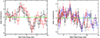 |
Fig. 3. Confidence contours showing deviations from the continuum model described in Sect. 4.1 in the soft (left) and hard (right) band. Black contours show Δ𝒞 = +0.5 while the colored contours show Δ𝒞 = −2.3 (cyan), −4.61 (blue), −9.21 (green), −13.82 (red), −18.42 (magenta), corresponding to a significance of 68%, 90%, 99%, 99.9%, and 99.99% for two parameters. In both panels, the main transitions from ionized Ne and Fe are labeled at their rest-frame energies. |
The spectral scan confirms the presence of a highly significant positive residual at ∼1.1 keV rest-frame (Figure 3, left), with a blueshift with respect to the most prominent lines expected in this region of the spectrum (namely ionized Ne and Fe lines) of the order of vout = 3 − 4 × 10⁴ km s−1. We also observe a strong absorption feature at higher energies, drawing a clear P-Cygni-like profile. If associated with the most prominent NeIX-X (at 0.91–0.92 and 1.02 keV rest-frame) and FeXVIII-XX (at 0.87 and 0.97 rest-frame) lines, the outflow velocity implied by the absorption feature would be in the range vout = 0.24 − 0.33c. The association with Fe L edges at 0.71–0.85 keV or with the blend of photoexcitation lines forming an unresolved transition array (UTA) at similar energies (Behar et al. 2001; Sako et al. 2001) would imply an even larger outflow velocity. These residuals are reminiscent of what observed in other similar targets like PDS456 (Reeves et al. 2016, 2020) and PG 1211+143 (Reeves et al. 2018b), where, thanks to high-resolution spectra from XMM-Newton RGS, similar emission and absorption features are resolved into multiple Fe and Ne highly ionized lines blueshifted by outflow velocities of ∼0.26c and ∼0.06c respectively, or IRAS 13224-3809 where Ne/Fe blended lines with outflow velocity of ∼0.25c are detected through principal component analysis (Parker et al. 2017).
In the hard band (Figure 3, right), two distinct, highly significant absorption features are observed around 9 and 11 keV. Both features can be attributed to a single outflow component with vout ∼ 0.27c if the 9.1 keV feature is associated with a blend of Fe XXV Heα and FeXXVI Lyα (at 6.70 and 6.97 keV rest-frame) and the 11 keV feature with a blend of Fe XXV Heβ and XXVI Lyβ (at 7.89 and 8.27 keV rest-frame).
We note the lack of a prominent Fe Kα line at 6.4 keV, in agreement with the low reflection measured in Sect. 4.1, while we observe highly significant positive narrow residuals at ∼6 and ∼7 keV. If the latter is attributed to Fe XXV/XXVI Kα lines, the derived blueshift is in the range vout = 5 − 17 × 103 km s−1. The presence of FeXXV/XXVI emission lines would be in agreement with the high ionization found using the xillver model for the reflector (see Sect. 4.1).
The ∼6 keV feature instead would require a substantial redshift, i.e., inflow velocity of up to 3 − 4 × 10⁴ km s−1 if associated with highly ionized Fe. Alternatively, the whole feature can be interpreted as a broad emission feature modified by self-absorption from low-velocity ionized components, as often observed in UV and soft X-ray lines (Costantini et al. 2007; Pounds & Vaughan 2011).
We also note negative residuals from pn and MOS1+2 around ∼10 keV rest-frame. These are, however, at different energies in the two sets of EPIC cameras and not seen at all by NuSTAR. The difference in energy between the pn and MOS1+2 features is of the order of ∼200 eV, which is much larger than the energy cross-calibration uncertainties expected between the two types of XMM-Newton cameras (a few tens of eV at these energies, Saxton & Stuhlinger, priv. comm.). Therefore, we conclude that these are most likely spurious features. Indeed, by running the spectral scan simultaneously on all the spectra, as explained above, we do not find any significant feature at ∼10 keV rest-frame.
As shown in Figure 1b, there are less prominent negative residuals between 2 and 5 keV. A spectral scan in this band reveals absorption features at ∼1.9, 2.7, and 3.4 keV rest frame at a significance of ∼90 − 99% confidence level. These are tentatively associated with Mg XII, Si XIV, and S XVI Lyα lines (at 1.47, 2.00, and 2.62 keV rest-frame respectively), assuming a blue shift of ∼0.27c (see Appendix A) as derived above for the 9 − 11 keV features. Indeed, modeling the hard band features with a single XSTAR table as discussed in Sect. 6 will also fit and remove these residuals.
Finally, there are noticeable negative residuals at ∼14.6 keV. Since only the NuSTAR spectra are available at these energies, the significance of the feature is quite low (∼95% confidence level from the spectral scan). If associated again with a blend of Fe XXV/XXVI Kα, the observed energy would imply an unprecedented outflow velocity of vout ∼ 0.63c, similar to the extreme wind velocity found in some of the observations of APM 08279+5255 (Chartas et al. 2009) and more recently in NGC 2992 (Luminari et al. 2023). The presence in IRASF11119 of a beamed radio jet with outflow velocity estimated to be > 0.57c (Yang et al. 2020) opens up the interesting possibility that we may observe signatures due to outflowing jet material, as tentatively reported in a handful of sources but never confirmed (Yaqoob et al. 1999; Wang et al. 2005; Zheng & Wang 2008), and suggested to explain the fastest UFOs seen in APM 08279+5255 (Zheng & Wang 2008). A thorough reanalysis of the Suzaku and NuSTAR spectra from Tombesi et al. (2015) and Tombesi et al. (2017) to explore the persistence and variability of all the features discussed above will be presented in Paper II.
5. Gaussian line properties and significance
To constrain the properties – energy, width, intensity – and the significance of the putative emission and absorption features identified in Sect. 4.2, we model each line with a Gaussian component, either in emission or absorption. The best-fit parameters of each Gaussian, labeled Emi or Absi for emission and absorption, respectively, and ordered by increasing energy, are reported in Table 2. The global fit statistics of the model comprising three emission and three absorption Gaussian lines, added to the broadband continuum, is 𝒞−stat = 392.47 for 363 d.o.f. with a significant improvement on the fit quality (see Figure 1c). Adding Gaussian emission and absorption lines to model the main residuals identified in Sect. 4.2 does not significantly impact the continuum best-fit values, which are therefore not reported in Table 2.
Best-fit parameters and significance of the Gaussian emission and absorption lines.
The location of the Gaussian lines is well constrained, with errors on the line energy of a few % in all cases. The width of the lines σwidth is consistent with a narrow, unresolved line in all cases except for the absorption line at 9 keV ( eV). When the line is consistent with being unresolved, we freeze the σwidth to its best-fit value. The equivalent width (EW) of the emission lines is in the range EW ∼ 75 − 120 eV, while the absorption lines at 9–11 keV have EW ∼ −230 eV. The absorption line in the soft is, instead, shallower with EW ∼ −30 eV.
As a first assessment of the line significance, we compute the Δ𝒞 between the best fit with and without each Gaussian line and the F-test null hypothesis probability considering two more free parameters (energy and normalization) for all cases except the absorption line at 9 keV, where also the width of the line is a free parameter. The improvement in the fit statistic Δ𝒞 is reported in Table 2 for each emission or absorption line. Pℱ, defined as 1 − Pnull where Pnull is the null hypothesis probability computed from the F-test, is also reported. All the lines are highly significant, with Pℱ > 99.9%, the weaker one being the feature at 11 keV, as also shown by the contour plots in Sect. 4.2. It is, however, well known that deriving the significance of additional components using the F-test is not appropriate when looking at emission/absorption lines (Protassov et al. 2002; Markowitz et al. 2006), as the null model is at the boundary of the parameter space (i.e., line normalization equal to 0). Furthermore, the results from the F-test tend to overestimate the significance of these components as they do not consider the full range of energies where a line might be observed by chance, the so-called look-elsewhere effect.
For this reason, we carried out a more rigorous test to assess the significance of the line based on Monte Carlo (ℳ𝒞) simulations (see, e.g., Porquet et al. 2004; Miniutti & Fabian 2006; Tombesi et al. 2010; Gofford et al. 2013; Matzeu et al. 2023 for a similar approach). The details of the simulations can be found in Appendix B. The goal of such simulations is to derive the significance of each added component Pℳ𝒞, defined as  where N is the number of simulated spectra showing a random fluctuation larger than the one observed in the data and S the total number of simulated spectra. The values of Pℳ𝒞 derived with this approach are reported in Table 2. None of the 1000 realizations in the soft and hard bands show a Δ𝒞 greater than the one observed for Em1, 2, 3 and Abs2 leading to Pℳ𝒞 > 99.9% for all these features, while Pℳ𝒞 = 99.8% for the remaining two absorption features.
6. Ultra fast outflow modeling
In the following, the same continuum model and emission lines described above are adopted, while the absorption lines are replaced by absorption tables from two different outflow templates. The continuum and emission line best-fit parameters are re-fitted to accommodate changes in the global fit.
6.1. XSTAR tables
As a first step, we adopt absorption tables created with the XSTAR photo-ionization code (Bautista & Kallman 2001; Kallman et al. 2004). This allows us to constrain the physical properties of the absorbing medium and, in particular, the ionization parameter (ξ), the column density (NH), and the outflow velocity (vout).
We start from the broadband continuum model described in Sect. 4.1. The XSTAR table modeling the WA and the three emission lines described in Sect. 5 are kept in the model, while the three absorption lines are removed and replaced by two XSTAR tables, as both the features at ∼9 and ∼11 keV can be modeled with the same highly ionized dense gas layer. We used the tables created with the XSTAR suite v2.54a for the SUBWAYS sample (Matzeu et al. 2023), which cover a wide range of column densities (log(NH/cm−2) = 23 − 24.3) and ionization parameters (log(ξ/erg cm s−1) = 2 − 8). These were generated for power-law SED of Γ = 2 input spectrum and an ionizing luminosity of Lion = 1 × 1045 erg s−1, well matched with the values observed in IRASF11119.
One of the input parameters needed to create the tables is the turbulent velocity vturb. To determine which input vturb is better suited to fit the observed features, we tested different tables with input vturb in the range 103 − 104 km s−1. We found that vturb = 3000 km s−1 and vturb = 1000 km s−1 reproduce best the observed hard band and soft band features, respectively. Therefore, in the following, we use the pre-compiled tables with such velocities. It is important to note that these values are lower than what can be derived at face value from the σ best-fit values of the Gaussian lines reported in Table 2 (∼8000 km s−1). This is because, in that approach, a single Gaussian profile is used to fit what is, in reality, the blend of multiple features: Fe XXV/XXVI Heα and Lyα in the case of the 9 keV feature, and several Fe and Ne lines in the case of the 1.3 keV feature.
One absorption table has a high best-fit column density and ionization parameter, as these are needed to reproduce the two main features in the hard band through a blend of Fe XXV/XXVI Heα-Lyα and Heβ-Lyβ transition pairs. The outflow velocity is vout = 0.27 ± 0.01c, falling in the Ultra Fast Outflow regime. We labeled this component as UFOH as it represents the high-ionization UFO component.
The soft feature instead is reproduced by a relatively low column and low ionization gas layer, with best-fit values typical of warm absorbers (Piconcelli et al. 2005; McKernan et al. 2007). The outflow velocity, vout = 0.30 ± 0.01c is, however, much higher than the typical WA and well within the UFO regime. We labeled this component as UFOL as it represents the low-ionization counterpart of the UFO. The two velocities are statistically self-consistent, as shown in Figure 4, right, suggesting that the two components are part of the same outflow. The best-fit parameters of the two XSTAR tables are shown in Table 3, while Figure 4, left, shows the confidence contours of log(NH) vs. log(ξ) for the two tables, while the residuals with respect to this model are shown in Figure 1d.
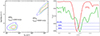 |
Fig. 4. Left: confidence contour levels of the column density NH and the ionization parameter log(ξ/erg cm s−1), for the best-fit model with two XSTAR tables, one with vturb = 1000 km s−1 for the low-ionization table UFOL and one with vturb = 3000 km s−1 for the high-ionization UFOH one. Right: contour plot of the outflow velocity for the UFOH in red and for UFOL in green. The blue lines mark one parameter’s 90, 99, and 99.9% confidence levels. |
Continuum and XSTAR absorption table best-fit parameters.
The column density of the UFOH component is at the limit of the range explored by the XSTAR tables adopted, up to NH = 2 × 1024 cm−2. Above this value, the derived intrinsic luminosity would be unreliable as XSTAR does not take into account Compton scattering. Log(NH) and log(ξ) of the highly ionized gas are also strongly correlated, as higher ionization states produce weaker absorption troughs that, in turn, can accommodate larger columns to fit the same observed features.
The outflow velocities of both UFOL and UFOH are well within the UFO regime (vout > 104 km s−1) and on the high-velocity tail of the distributions observed in the local Universe (Tombesi et al. 2010; Gofford et al. 2013; Igo et al. 2020) and up to z = 0.5 (Matzeu et al. 2023): there are only 3 cases of UFO with faster velocities among the 65 individual detections in the spectra of the four combined samples, with several sources in common. In Figure 5, we show the best-fit model with the three XSTAR tables described above. We labeled in red the main absorption features produced by the WA table, in green those relative to the UFOL table, and in blue those relative to the UFOH table. The ions producing the main features are also labeled.
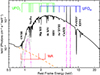 |
Fig. 5. Unfolded best-fit model (black) in νF(ν) including three XSTAR absorption tables. The emission lines are shown in magenta, and the scattered emission is in orange. The main absorption features due to the WA, UFOL, and UFOH are labeled in red, green, and blue, respectively. The ions producing the most prominent features are labeled in black. |
We stress that only one XSTAR table is needed to model both the 9 and 11 keV features, and the same table also models the less significant residuals observed at 2, 2.7, and 3.4 keV (see Appendix A). As a result, the Δ𝒞 obtained when adding this component is Δ𝒞 ∼ 42 for three more free parameters. This is significantly larger than the Δ𝒞 associated with each of the Gaussian lines reported in Table 2, boosting the overall significance with respect to the results derived in Sect. 5. Adding the XSTAR table for the UFOL gives a Δ𝒞 ∼ 15, comparable with the value derived for a simple Gaussian line. The global fit statistics of the model comprising three emission Gaussian lines and three XSTAR absorption tables for WA, UFOL and UFOH is 𝒞−stat = 389.3 for 369 d.o.f.
In order to have a rough estimate of the covering fraction of the wind, we followed the approach described in, e.g., Nardini et al. (2015) and Reeves et al. (2016), fitting the excess emission in the hard band (after removing the Gaussian lines at 6 and 7 keV) with an additive table created by XSTAR together with the absorption tables, that models the reflected emission from the wind. Indeed, the reflected emission table is able to model the emission feature at 7 keV with emission from the FeXXVI Lyα line, whose intensity is actually driving the normalization of the whole reflected component (see Nardini et al. 2015 for a similar case on PDS456).
The normalization k of the reflected component is defined by XSTAR in terms of k = fL38/D2(kpc) where L38 is the ionizing luminosity in units of 1038 erg s−1, and D(kpc) is the distance to the quasar in kpc and f is the covering fraction of the gas with respect to the total solid angle, in terms of f = Ω/4π. Thus, by comparing the predicted normalization for a fully covering shell of gas versus the observed normalization (kxstar), the covering fraction of the gas can be estimated. For IRASF11119, with Lion = 4 × 1045 erg s−1 at a luminosity distance of D = 779 Mpc, the observed value of the normalization ( ) implies a covering fraction of f > 0.4.
In Figure 6, we show the distribution of log(NH) vs. vout (left) and log(ξ) vs. vout (right) best-fit values of the three XSTAR absorption tables adopted here and compare them with the typical UFO and WA parameter spaces (cyan and green, respectively) taken from the literature (e.g., Tombesi et al. 2013; Gupta et al. 2013a; Serafinelli et al. 2019). While the WA and UFOH components fall in the respective classical regions, the outflow observed in the soft band falls in a poorly populated region of low ionization/low column clouds outflowing at velocities typical of UFOs.
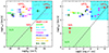 |
Fig. 6. log(NH) vs. vout (left) and log(ξ) vs. vout (right) for the WA, UFOL, and UFOH components of IRASF11119 (red diamonds). The known soft-band detected fast winds from the literature are shown with colored points: light green (Gupta et al. 2013b); cyan (Gupta et al. 2015); sky blue (Longinotti et al. 2015); magenta (Reeves et al. 2016); blue (Pounds et al. 2016); orange (Jiang et al. 2018); yellow (Serafinelli et al. 2019); dark green (Krongold et al. 2021). The low-velocity WAs region (green), UFOs region (cyan), and the correlation fits linking low-velocity WAs and UFOs (dashed black lines) are derived from Tombesi et al. (2013). |
This UFOL component represents a promising new example of a poorly explored phase of the UFO phenomenon, with only about a dozen other sources known to date to show such features mainly detected in high-resolution grating spectra. These features are thought to be produced by ISM clouds at great distances from the SMBH (tens/hundreds of parsec, also referred to as ‘meso-scale’), entrained by the advancing outer shock of the nuclear UFO (e.g. Faucher-Giguère & Quataert 2012). Alternatively, they may represent the imprint of the UFO gas itself cooling down and fragmenting (e.g. Takeuchi et al. 2013). In the latter case, the expected distances would be much smaller, of the order of hundreds of Rg. Variability of these features may help discern between the two interpretations, as in the case of PG 1211+143 (Reeves et al. 2018b), a thorough search for long and short-term variability of both the UFO features presented here will be addressed in Paper II.
The growing number of highly accreting sources in which this new outflow phase has been discovered, possibly located at the meso-scale between the nuclear UFO and the larger scale WA, supports the idea that all these different wind components are, in fact, different phases of a single phenomenon expanding from the inner regions of the AGN into the host galaxy. In particular, this may be interpreted as the interface zone in which the nuclear UFO interacts with the clumpy regions at 10s–100s of pc distance, forming blobs of fast-moving but denser and colder gas. This picture agrees with predictions by models of self-regulating feedback mechanisms for the evolution of galaxies (Zubovas & King 2012; King & Pounds 2015; Gaspari et al. 2017).
It is interesting to note that, while in the case of ‘classical’ UFOs at the accretion disk scale, vturb is generally interpreted as a velocity gradient within the outflow (with values up to 10 000 km/s in the most extreme cases, e.g. Nardini et al. 2015; Tombesi et al. 2015), for the UFOL at larger scales vturb could really be interpreted as an indication of the amount of turbulence in the flow, as for sub-relativistic outflows, at least several 100 km/s of turbulence can be expected at large scales (Wittor & Gaspari 2020). Indeed, turbulence is key to having entrained outflows and thus generate different absorbers along the LOS, as found here: the stronger the turbulence, the larger the K-H instabilities, hence the entrainment (e.g. Gaspari et al. 2020).
6.2. Disk wind table
To model the UFO features, we also tested the publicly available4 DISK-WIND table of simulated radiation-driven wind spectra generated using the Monte Carlo radiative transfer code developed in Sim et al. (2008, 2010), Matzeu et al. (2022).
The DISK-WIND computes emission and absorption spectra arising from a smooth, steady-state, and bi-conical flow with an opening angle of 45 degrees. With such assumptions, we can provide a self-consistent treatment of both transmitted and scattered components from a realistic geometry that includes a radial-dependent ionization and velocity structure across the flow. We can probe the overall mass outflow rate, velocity, and viewing angle of classical UFOs. In this work, we adopted the fast32 grid, which assumes a lunching radius of 32 Rg. The parameters of the fit are:
-
The velocity parameter (fv), which relates the terminal velocity (v∞) of the wind to the escape velocity at the origin (vesc = (2GMBH/Resc)1/2) via fv = v∞/vesc. In the case of the fast32 grid adopted here, the inner edge of the wind is launched at Resc = 32 Rg and therefore vesc = 0.25c.
-
The line-of-sight inclination angle (μ) defined as μ = cos(θ) where θ is the angle between the observer’s line-of-sight and the polar z-axis of the flow.
-
The mass outflow rate (
 ), defined as
  , i.e., normalized by the Eddington limit, making this measurement black hole mass invariant.
 -
The ionizing luminosity (ℒX) defined as ℒX = (L2 − 10 keV/LEdd)×100, which is also normalized to the Eddington limit.
-
The photon index Γ of the power-law continuum, extrapolated over the 0.1 − 511 keV range, used to self-consistently compute the wind spectrum. We linked this parameter to the pexrav best-fit photon index, recomputed after including the DISK-WIND table.
More details on the DISK-WIND parameters are provided in Sect. 2 of Matzeu et al. (2022).
Together, fv and μ regulate the observed location and width of the absorption features produced by the outflowing gas: fv by setting the terminal velocity of the flow, while the launch velocity is fixed, and μ by setting which part of the flow is intercepted by the line of sight.  regulates the amount of material in the flow and, therefore, the depth of the absorption features. Finally, ℒX regulates the degree of ionization at the location where the l.o.s. intercepts the flow.
The DISK-WIND model is designed to reproduce the typical UFO absorption features observed in the hard band (i.e., high column and high ionization state). Even if the parameters  and ℒX cover a wide range of values (
![$ \mathcal{\dot M}_{\mathrm{w}}=[0.0196{-}1.287]{\dot M_{\mathrm{Edd}}} $](/articles/aa/full_html/2024/09/aa49194-24/aa49194-24-eq30.gif) and ℒX = [0.025 − 2.516]%LEdd) these intervals do not extend enough to the lower end to cover the parameter space needed to reproduce the UFOL feature observed in IRASF11119. Therefore, we adopt the DISK-WIND table to model only the UFOH features, replacing the relative XSTAR table, while we keep the rest of the model components described in Sect. 6.1.
and ℒX = [0.025 − 2.516]%LEdd) these intervals do not extend enough to the lower end to cover the parameter space needed to reproduce the UFOL feature observed in IRASF11119. Therefore, we adopt the DISK-WIND table to model only the UFOH features, replacing the relative XSTAR table, while we keep the rest of the model components described in Sect. 6.1.
The best-fit parameters results are reported in Table 4, while the best-fit model and residuals are shown in Figure 7. The continuum parameters are only marginally affected by replacing the XSTAR table for the UFOH with the DISK-WIND table, except for a significantly smaller scatter fraction. This is due to the fact that the whole primary continuum is suppressed by the obscuring materials in the wind, and the intrinsic, absorption corrected luminosity is higher: L2 − 10 keV = 5.4 vs. 1.2 × 1044 erg s−1. The WA and UFOS parameters are also only marginally affected with respect to the fit with the XSTAR tables.
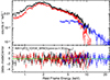 |
Fig. 7. XMM-Newton and NuSTAR spectra with the best-fit continuum model and residuals, for the model described in Sect. 6.2, where the DISK-WIND table replaces the UFOH XSTAR table. The colors are the same as in Figure 1. |
Best-fit parameters of the model where a DISK-WIND grid was used to replace the XSTAR table to model the UFOH features.
When fitted as free parameters, the wind terminal velocity and inclination angle are well constrained (see Figure 8 left): the line-of-sight intercepts the wind at an angle θ ∼ 58° from the vertical axis, where the flow has a wide range of velocities and ionization states, which blend the FeXXV and XXVI line pairs into two rather broad absorption features. fv ∼ 1.5 means that the inner edge of the wind is accelerated from vesc = 0.25c at the origin (Resc = 32 Rg) to v∞ = 0.38.
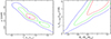 |
Fig. 8. Confidence contour levels of the DISK-WIND parameters fv vs. μ (left) and |


Due to interpolation limitations of the current DISK-WIND grids (Matzeu et al. 2022), it is recommended to freeze these two parameters to the closest grid point (μ = 0.525 and fv = 1.5, respectively, in this case) in order to get more reliable constraints on the other two parameters of interest  and ℒX. Figure 8, right, shows the results of this approach: the mass outflow rate is broadly consistent with the Eddington accretion rate (
 ), while the luminosity seen by the wind is ℒX ∼ 2.2%LEdd, which for a 2 × 10⁸ M⊙ BH translates into ℒX = 5.5 × 1044 erg s−1. This is a further indication that the absorption-corrected luminosity in the DISK-WIND fit case is higher than in the XSTAR fit (L2 − 10 keV = 5.4 × 1044 erg s−1) where Compton scattering is not included: the wind sees a factor ∼4 higher intrinsic luminosity with respect to the uncorrected, observed value, as the intrinsic luminosity is affected by obscuration by the thick wind itself.
Applying a bolometric correction of kbol ∼ 50 − 60, proper for such luminosity (Marconi et al. 2004; Duras et al. 2020), we derive a bolometric luminosity Lbol ∼ 3 × 1046 erg s−1. This is a factor ∼2 larger than the one derived from the IR emission (Veilleux et al. 2013), consistent within the BH mass and bolometric correction factor uncertainties.
The fit quality is comparable to the fit with three XSTAR tables for one more free parameter. In fact, the residuals for the two fits are indistinguishable (see Figure 1d and Figure 7). We note, however, that neither the XSTAR tables nor the DISK-WIND one are able to perfectly model the feature at 11 keV, while they do model the one at 9 keV. This may be related to the fact that the wind is probably more complex in terms of clumpiness, velocity, and ionization structure than the simple geometries assumed in both these approaches.
The DISK-WIND table also includes emission from the outflowing gas outside the line-of-sight. This produces a broad emission between 6 and 7 keV rest-frame in a classical P-Cygni profile, with an intensity that depends mainly on the system’s geometry. In the best fit described above, this emission partly accounts for the narrow emission modeled with Gaussians at 6 and 7 keV.
We will present in Paper II results on the physical properties of the wind derived using state-of-the-art wind models, such as WINE (Luminari et al. 2021), that computes both absorption and emission from the wind in a bi-conical geometry, and XRADE (Matzeu et al. 2022), an emulator of DISK-WIND developed to solve interpolation limitations of this model.
7. Properties of the X-ray corona
As described in Sect. 4.1, the primary power-law in IRASF11119 (Γ ∼ 2) is modified by an extremely low high-energy cutoff of the order of ∼30 keV, plus negligible reflection. By adding the XSTAR or DISK-WIND absorption tables, the Ecut value shifts to an even lower value (Ecut ∼ 25 keV, see Table 3 and Table 4), among the lowest reported in the literature (Kara et al. 2017; Tortosa et al. 2023). Figure 9 shows the contour plot of the primary power-law high energy cutoff vs. photon index from the best-fit model with the UFO XSTAR absorption tables, described in Sec 6.1, while the gray contours show the results from the continuum model only, described in Sect. 4.1.
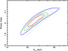 |
Fig. 9. Confidence contour levels of the high energy cutoff vs. the photon index. The colored contours refer to the best-fit model with two UFO XSTAR absorption tables, described in Sect. 6.1, while the gray contours show the results from the continuum model only, described in Sect. 4.1. |
We note that the high energy cutoff and the photon index of the primary power-law modeled with pexrav are correlated, as a flatter photon index requires an even lower cutoff to account for the observed lack of hard band counts. Also, the addition of absorption tables, such as XSTAR or DISK-WIND, shifts the Ecut to lower values, as part of the soft emission is absorbed by the wind, and therefore, the continuum in the hard band can be even steeper. However, the results are consistent with each other within 1σ confidence level.
Thanks to the advent of the NuSTAR hard X-ray imaging telescope (Harrison et al. 2013), the high energy cutoff is now known with unprecedented accuracy for tens of nearby bright Seyfert galaxies (e.g. Fabian et al. 2015; Tortosa et al. 2018; Kamraj et al. 2018; Baloković et al. 2020; Kang & Wang 2022). Figure 10 shows these measurements as a function of X-ray luminosity for local Seyferts (gray circles, from the updated sample in Bertola et al. 2022) and the binned results from the BAT-selected sample of Ricci et al. 2018 (magenta triangles). The few luminous quasars at z ≳ 0.5 for which such measurement has been possible so far are shown in green (Kammoun et al. 2017, 2023; Lanzuisi et al. 2019; Bertola et al. 2022; Marinucci et al. 2022), while PDS456 (Reeves et al. 2021) is shown in cyan. The yellow/orange areas show the runaway pair-production region (Fabian et al. 2015), translated into directly observable quantities for different geometries of the corona and assuming different BH mass values, shown with different line styles (see Lanzuisi et al. 2019 and Bertola et al. 2022 for details). The Ecut measured for IRASF11119 (see Figure 9) is shown by the red cross, where the luminosity is the average of the two different measurements obtained from the XSTAR and the DISK-WIND fits, and the error bars show the range covered by them. The target shows one of the lowest Ecut reported in the literature at all luminosities.
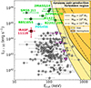 |
Fig. 10. High-energy cutoff vs. intrinsic luminosity for local Seyferts measured with NuSTAR (gray dots, from the updated sample of Bertola et al. 2022), and the binned results from the BAT-selected sample (magenta downward pointing triangles, Ricci et al. 2018). Green data points show results for luminous quasars at z ≳ 0.5: pentagon from Kammoun et al. (2017); squares Lanzuisi et al. (2019); star Bertola et al. (2022); plus Marinucci et al. (2022); right-ward triangle Kammoun et al. (2023). PDS456 (Reeves et al. 2021) is shown in cyan and IRASF11119 in red. The different intrinsic luminosities obtained from the XSTAR and DISK-WIND fits are shown by the vertical error bar. The yellow/orange areas show the runaway pair-production forbidden region (Fabian et al. 2015; Lanzuisi et al. 2019) for different geometries and BH masses. |
Several examples are known of strong X-ray UFOs detected in sources with relatively cool coronae, such as PDS456 (Ecut ∼ 50 keV, Reeves et al. 2021), or LBQS 1338-0038 (Ecut ∼ 50 keV; Matzeu et al. 2023, Matzeu et al. in prep.). The super-Eddington accreting NLSy1s I Zw 1 (Ding et al. 2022) and IRAS 04416+1215 (Tortosa et al. 2022) show even lower Ecut values (∼15 keV) and are again associated with the presence of UFOs. These findings indicate a possible correlation between strong nuclear outflows and a cold corona or soft continuum, often associated with highly accreting/super Eddington and NLSy1 sources.
High Eddington rates, by definition, promote strong radiation-driven winds and, at the same time, increase the efficiency of the corona cooling, as the Compton cooling is proportional to the inverse of the radiation energy density. In fact an anticorrelation between Ecut and λEdd has been indeed observed in Ricci et al. (2018) based on BAT data, even if such anticorrelation has not been confirmed in later studies based on NuSTAR data (Hinkle & Mushotzky 2021; Kamraj et al. 2022; Serafinelli et al. 2024). In a systematic study of super-Eddington sources Tortosa et al. (2023) indeed found indication of softer spectra and the presence of ionized outflows in most of them, but only two out of eight show low Ecut values.
On the other hand, a colder corona or softer power-law may promote the formation of nuclear winds by preventing the gas surrounding the inner disk from being over-ionized (Proga & Kallman 2004; Nomura et al. 2020; Matzeu et al. 2022),
In particular, in case of a high accretion rate, it has been suggested (e.g. Sądowski & Narayan 2016; Kubota & Done 2019) that the inner standard accretion disk puffs up due to the high radiation pressure of UV photons. The inner puffed-up disk increases the UV/soft X-ray flux seen by the corona, leading to more efficient cooling and, at the same time, shields the rest of the inner accretion disk from hard X-rays, preventing over-ionization and allowing for inner/faster winds to be launched. This mechanism has been invoked for z > 6 QSOs showing a correlation between photon index and nuclear wind (observed as CIV emission line outflowing components) outflow velocity (Tortosa et al. 2024).
The connection between a steep continuum and the presence of strong/persistent nuclear outflows may also have important implications for the impact of AGN feedback in the early Universe, given the recent results on the spectral steepening in the z > 6 QSO HYPERION sample (Zappacosta et al. 2023). A systematic study of the incidence of UFO features as a function of coronal properties and the Eddington ratio is thus needed to explore the link between all these aspects of SMBH accretion, but is beyond the scope of this paper.
8. Large-scale wind properties from optical spectroscopy
The optical spectrum of IRASF11119 shows peculiar features that have been only partially analyzed in the literature (Lípari et al. 2003; Rupke et al. 2005). We reanalyzed the publicly available 2013 SDSS-eBOSS spectrum of IRASF11119 by performing simultaneous multicomponent fitting using the code PyQSOFit (Guo et al. 2018). We model the continuum with a polynomial component and FeII emission templates from Boroson & Green (1992). Galactic extinction is also included through the dust-reddening maps of Schlegel et al. (1998). We simultaneously model emission lines with a combination of narrow and broad Gaussian functions. These include:
-
Six narrow (FWHM < 500 km/s) lines: Hα (6563 Å), Hβ (4861 Å), and [OIII] (4959,5007 Å) and [NII] (6549,6584 Å) doublets. The ratios of the [OIII] and [NII] doublets were both set to be 1:2.99 from atomic physics.
-
Two very broad (FWHM > 2000 km/s) lines to account for the Hα and Hβ Broad Line Region (BLR) emission.
-
Six broad (500 km/s < FWHM < 2000 km/s) lines to account for outflows or to better describe the BLR emission profile, which is known to be poorly reproduced with only one Gaussian line. The ratios of the [OIII] and [NII] doublets were constrained as above.
We constrain the width of the narrow components to be the same, and we do so for the broad components as well. Initially, we also request for the line centroid offset to be the same for all the lines belonging to the same group (narrow, broad, and very broad), as it is a well-tested recipe used in the characterization of galactic outflows (e.g. Brusa et al. 2015; Perna et al. 2015). However, these constraints appear to be too harsh to model the complex kinematics revealed by the optical spectrum, and we, therefore leave the offset free to vary from one line to the other in the same group.
IRASF11119, in fact, is a “blue outlier”, meaning that the peak of the [OIII] emission lines is blue-shifted by more than 250 km/s with respect to the Balmer lines (Zamanov et al. 2002). These rare sources (3–5% of optically selected AGN) are typically associated with low-mass, highly accreting AGN and with the presence of nuclear outflows (Marziani et al. 2003, 2016). Indeed, while the Hβ and Hα peak at wavelengths corresponding to z = 0.190, the [OIII] lines peak corresponds to z = 0.187, with little to no narrow emission at the expected wavelength for z = 0.190. The whole [OIII] emission can, therefore, be interpreted as due to outflowing material. We decided to untie the centroid offset of the lines in the [OIII] doublet from the rest of the narrow lines while keeping them tied to each other. In this way, both narrow and broad [OIII] lines account for outflow emission. The fit results are shown in Fig. 11. For the BLR, the FWHM of the broad and very broad components combined is ∼2500 km/s, comparable with the 2000 km/s adopted in Nardini & Zubovas (2018) from which they derived a black hole mass of MBH ∼ 2 × 10⁸ M⊙.
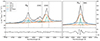 |
Fig. 11. Hβ, [OIII], and Hα regions of the optical spectrum of IRASF11119. The observed spectrum is plotted in gray, while the best fit is shown as the black dashed line. Different model components are traced by lines of different colors, as indicated by the label. The vertical dashed lines indicate the rest-frame wavelength for each labeled emission line, for z = 0.187. In the bottom panels, residuals are plotted. Note that the Hα shows significant residuals, possibly due to the blending with the [NII] doublet, but this effect is negligible for our goals. |
In addition to the previously reported lines, we also detect emission from forbidden lines of different ionization levels such as [SII], [SIII], [OII], [NeIII], and [NeV]. For each line, we measure a non-negligible velocity shift with respect to the systemic redshift obtained from the Balmer lines, and we found a clear positive trend between this shift and the ionization level of the gas responsible for each line. A similar trend is usually observed between the [OIII] and the Balmer lines (Veilleux 1991; Zamanov et al. 2002; Eracleous & Halpern 2004; Hu et al. 2008). This is interpreted in the context of decelerating outflows in a stratified medium, photoionized by the AGN (Veilleux 1991; Zamanov et al. 2002; Komossa et al. 2008; Spoon & Holt 2009): More highly ionized species correspond to gas closer to the nuclear AGN, and the observed trend indicates a stratification of the gas velocity, decreasing at larger radii.
To test this hypothesis, we computed the ionization parameter at which each ion has its peak of relative abundance using CLOUDY, v23.0 (Chatzikos et al. 2023), assuming a fixed gas density of nH = 103 cm−3 and the SED of IRASF11119 as the ionizing continuum. We can then convert this into a distance from the ionizing source using the definition of the ionization parameter ξ ≡ Lion/nr2 where n is the number density of the absorbing material, and r is the distance.
The results are shown in Figure 12. Given the low S/N levels of the SDSS spectrum, the [NeIII], [OII], and [SII] doublets are fitted with pairs of lines at a distance fixed to the lab value so that we derive a single velocity offset value for each doublet. With our assumptions, we derive that the high-ionization line [NeV] is produced by gas at ∼200 pc from the center, outflowing at velocities of ∼1500 km/s, while [OII] and [SII] doublets are produced by gas at few kpcs (i.e. at scales comparable with the whole host galaxy) and at that point the outflow velocity has dropped to ∼200 km/s. The red curve is a power-law fit to the data in the form vout = a × rb + c. The best-fit slope is b = 0.20 ± 0.07. The dashed gray line shows a dependency of the form r0.5, i.e., a purely ballistic trajectory. The best-fit relation is slightly flatter but consistent with the ballistic curve. AGN radiatively driven large-scale winds are expected to be energy-conserving at these scales and to propagate with a flatter velocity gradient, thanks to the pressure support of the hot wind (see, e.g., Fabian et al. 2015). This is shown by the green dotted curves taken from the analytic treatment presented in Faucher-Giguère & Quataert (2012), with parameters Lbol = 1046 erg s−1, vin = 0.1c, and central density n0 = 10 − 100 cm−3.
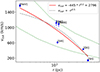 |
Fig. 12. Distance from the ionizing source vs. velocity offset for different emission lines (labeled) modeled in the SDSS spectrum. The distance is derived from the ionization level at which each ion has the peak of relative abundance. The red curve is a power-law fit of the form vout = a × rb + c with the best-fit slope b = 0.20 ± 0.07. The gray dashed line shows a curve with a slope fixed to b = 0.5, the value for a simple ballistic trajectory. The dotted green curves are taken from the analytic treatment of an expanding AGN-driven wind presented in Faucher-Giguère & Quataert (2012), for vin = 0.1c, and central density n0 = 10 (top) and n0 = 100 (bottom) cm−3. |
We stress that different assumptions on the value of the constant gas density can substantially change the results in terms of the radius of each ion, while the general trend of decreasing velocity at larger radii would remain. Introducing a radial-dependent density profile would change the slope of the curve, i.e., flatter curves for density decreasing with radius. A more detailed investigation taking into account the possible effects of a clumpy medium and of the different line critical densities is beyond the scope of this paper.
9. Energetics of the outflow components
9.1. Nuclear Outflow
To derive the energetics of the nuclear outflow we followed a standard approach starting from the best-fit values of the XSTAR tables described in Sect. 6.1. A lower limit of the distance between the central BH and the absorbing gas layer can be inferred from the radius at which the observed outflow velocity along the line of sight corresponds to the escape velocity:
For the derivation of the maximum distance of the absorber, the definition of the ionizing luminosity Lion is often used, which is the source ionizing luminosity integrated between 1–1000 Ryd. We computed Lion from the broadband SED derived in Sect. 3, i.e. Lion = 4 × 1045 erg s−1. We use again the definition of the ionization parameter, ξ ≡ Lion/nr2. As the size of the absorber cannot exceed its distance to the black hole, NH ≃ nΔr < nr, we obtain:

In the case of IRASF11119, rmin ∼ 13RS and rmax ∼ 530RS for the UFOH absorber. Following the same approach for the UFOL and WA absorbers would translate into rmin ∼ 11RS and rmax ∼ 107RS or ∼650 pc for UFOL and rmin ∼ 105RS or a few pc, and rmax ∼ 109RS or ∼104 pc for the WA. These simplified definitions are, therefore, clearly not useful for these lower ionization absorbers since the values of rmin and rmax span several orders of magnitudes from the vicinity of the SMBH to the outskirts of the host galaxy.
In fact, estimates of the location of the WA vary significantly in the literature, possibly reflecting the intrinsic multiphase, multitemperature nature of these outflows (e.g. Krolik & Kriss 2001; Krongold et al. 2007; Di Gesu et al. 2013; Laha et al. 2021). Studies from extensive multiwavelength campaigns on single sources and based on variability (e.g. Kaastra et al. 2011) locate the WA at tens of pc from the SMBH (Kaastra et al. 2012, 2014). The location of the gas responsible for the UFOL is even more uncertain. It has been suggested, and in at least one case derived from variability arguments (Serafinelli et al. 2019), that these low column and ionization UFOs may be located at the interface between the nuclear UFO and the WA, i.e., hundreds of parsecs from the SMBH (e.g., Gaspari et al. 2020), while the interpretation as the UFO gas cooling down and fragmenting (e.g., Takeuchi et al. 2013) implies much smaller distances (hundreds of Rg).
In any case, it is to be expected that the energy carried by both the UFOL and the WA is only a small fraction of that of the “classical” UFO, as the column density is 2–3 orders of magnitude lower, and for WA the outflow velocity is negligible (see Reeves et al. 2018b for a notable exception). Therefore, in the following, we focus on the derivation of the energetics of the UFOH component only.
We compute the mass outflow rate through the standard expression:
following Tombesi et al. (2012), Gofford et al. (2013), Nardini & Zubovas (2018) and assuming solar abundances, full ionization, and neglecting more complex geometrical descriptions. mp is the proton mass, Ω is the solid angle subtended by the wind, and NH, vout and r are its column density, velocity, and radius. We adopt a solid angle ΩFeK/4π = 0.5 consistent with the value derived in Sect. 6.1, and comparable to the one derived from the P-Cygni profile in PDS 456 (Nardini et al. 2015) and from population studies (Tombesi et al. 2010; Gofford et al. 2013).
We compute Ṁout using the lower limit reported in Table 3 as the upper boundary is unconstrained. The measured vout is also a lower limit since the observed value is only the component along the l.o.s. Consequently, we compute Ṁout only for the rmin as we can only derive a lower limit of this quantity. We further note that taking into account special relativistic effects, the observed NH must be corrected to take into account the reduction of the optical depth of the outflowing gas for increasing vout (e.g. Luminari et al. 2020). This velocity-dependent correction is of the order of ∼2 for an outflow velocity of 0.27c. In the following, we take into account this correction when computing the wind energetics. We therefore obtain Ṁout > 2.1 M⊙/yr or Ṁout ≳ 0.49 ṀEdd or Ṁout ≳ 0.82 Ṁacc.
In the classical treatment, we can then derive the mechanical power as 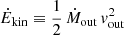 and the outflow momentum rate Ṗout ≡ Ṁout vout. The correction on Ėkin due to the special relativistic formula (γ−1)Ėoutc2 (Saez & Chartas 2011; Luminari et al. 2021) is minor since the Lorentz factor γ is ∼1.04 for vout = 0.27c. The results for UFOH are therefore Ėkin > 0.32 Lbol and Ṗout > 2.26 Lbol/c.
In the DISK-WIND fit instead, it is possible to directly derive the mass outflow rate and the terminal velocity of the wind, corrected for projection effects, as  , fv, and μ are parameters of the fit. We use the Ṁout derived in Table 4,
 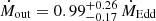 , that for a MBH = 2 × 10⁸ M⊙ translates into
 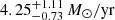 or
or  given the observed mass accretion rate.
Therefore, in IRASF11119, as it happens in similar highly accreting sources (PDS456, PG 1211+143), the mass outflow rate is comparable with the mass accretion rate and close to the Eddington limit. This suggests that the accretion rate in the external part of the accretion disk is potentially higher than Eddington, and the outflow substantially contributes to keeping the effective accretion rate onto the SMBH below such a limit.
The derived terminal velocity is larger than the observed one obtained from the XSTAR fit. This is due to inclination (deprojection) effects and to the acceleration of the gas along the line of sight up to the maximum velocity. Also, this is the velocity corresponding to the inner edge of the wind (i.e., Resc = 32 Rg), while the outer edge (i.e., Resc = 48 Rg) has a lower terminal velocity of 0.3c. The mechanical power and outflow momentum rate are also higher than what was estimated from the XSTAR fit: 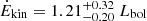 and
and 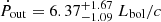 .
.
9.2. Large-scale ionized outflow
We analyze the kinematic of the large-scale outflow observed in the [OIII] emission in the SDSS spectrum using prescriptions well established in the literature (e.g., Cano-Díaz et al. 2012; Fiore et al. 2017). By assuming spherical geometry and constant density of the outflow, the mass outflow rate can be computed as  (see Lutz et al. 2020 for a discussion on the implication of different assumptions on outflow geometry and history). VOUT is the maximum outflow velocity, ROF is the outflow radius and MOF is the mass of the gas entrained in the outflow. We constrain ROF using the SDSS-BOSS fiber diameter (2″), which corresponds to 3.2 kpc at z = 0.190. This should be considered as an upper limit, and it is roughly consistent with what is derived in Figure 12 for the [OIII] radial extent. Therefore, ROF and MOF should also be considered upper limits.
The outflow velocity VOUT is estimated through non-parametric analysis in order to minimize bias arising from the fitting procedure. We compute both v02 and w80. v02 is the velocity corresponding to 2% of the flux for the [OIII]λ5008 line, with respect to the rest frame emission. w80 corresponds to the difference in velocity between 10% and 90% of the flux of the [OIII]λ5008 line. The second velocity estimator, w80, is thought to be more robust, as it takes into account a difference between velocities rather than just one measurement. However, it is not sensitive to the fact that the whole [OIII] emission is blue-shifted. Our estimate of VOUT is therefore v02 = 3053 ± 92 km/s, rather than w80 = 2264 ± 68 km/s.
The mass MOF is given by:
![$$ \begin{aligned} {M_{\rm OF}} = 5.3 \times 10^7 \frac{L_{44}(\mathrm{[OIII])} }{n_{\mathrm{e}_3}10^{[\mathrm{O/H} ]}} \, \mathrm M_{\odot } \end{aligned} $$](/articles/aa/full_html/2024/09/aa49194-24/aa49194-24-eq60.gif)
where L44([OIII]) is the luminosity of the [OIII]λ5008 line tracing the outflow in units of 1044 erg/s, 10[O/H] is the metallicity of the outflowing gas and ne3 is the electron density of the same gas in units of 1000 cm−3. Most authors estimate ne3 through the ratio R between the lines of [SII] doublet. However, in our case, the low S/N did not allow for robust measurement of R. In addition, this method has been shown to be biased towards lower densities, also in samples of AGNs with outflows (e.g., Baron & Netzer 2019; Davies et al. 2020). For these reasons, we conservatively assume the median density log(ne) = 3.7 ± 0.16 derived in Rose et al. (2018) using the Trans-Auroral Ratio (TR) which measures ne3 making use of the doublets [SII]λλ 4068, 4076, [SII]λλ 6717, 6731, [OII]λλ 3726, 3729, and [OII]λλ 7319, 7331.
The observed [OIII]λ5008 luminosity is L([OIII]) = 1.59 ± 0.11 × 1042 erg/s. However, the spectrum is reddened, as indicated by the Balmer decrement Hα/Hβ = 12.6 ± 2.9, which is > 3 − 4 times higher than the standard intrinsic value of 2.86 (Osterbrock 1989). By using the empirical approach presented in Calzetti et al. (1994), and using the extinction curve k(λ) found in Calzetti et al. (2000), we derive the corrected value of ![$ L(\mathrm{[OIII]})=1.61^{+1.46}_{-0.92} \times10^{44} $](/articles/aa/full_html/2024/09/aa49194-24/aa49194-24-eq61.gif) erg/s. Assuming solar metallicity, we derive
erg/s. Assuming solar metallicity, we derive 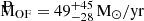 . This corresponds to a momentum outflow rate of
 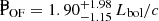 .
.
The energetics recently derived in Pan et al. (2019) using the same SDSS spectrum, along with dedicated NIR-MIR data, is higher by a factor ∼7 of the one derived above. This is partly due to the different assumed geometries: while we assume a uniformly filled spherical geometry, they assume co-spatiality and coupling of molecular, neutral, and ionized gas in a thin-shell geometry, which corresponds to higher mass outflow rates (e.g., Maiolino et al. 2012). More importantly, their modeling of the outflow combines information from molecular, ionized, and neutral phases of the gas. Consequently, their derived parameters are similar to those derived in Nardini & Zubovas (2018) for the molecular outflow alone, which is dominating the energetics at large radii. Our method, instead, by focusing on [OIII], probes the faster, lighter, and more highly ionized phase of the large-scale outflow.
9.3. Momentum boost diagram
Figure 13 summarises the results on the wind energetics derived for IRASF11119 (in red). The diamond shows the UFOH momentum rate derived from the XSTAR best-fit parameters, while the empty star shows the results from the DISK-WIND model fit. The empty pentagon shows the momentum rate of the large-scale ionized outflow observed in [OIII]. The filled circles show values from the literature, as recomputed in Nardini & Zubovas (2018). We note that the error bars on vout from the XSTAR fit presented in Figure 13 are much smaller than those used in Nardini & Zubovas (2018) and derived from the NuSTAR follow-up of 2016 (Tombesi et al. 2017), thanks to the much higher spectral quality and energy resolution of our data. On the other hand, the error bars on v∞ from the DISK-WIND fit are larger and more realistic than those obtained from the XSTAR fit, as the DISK-WIND fit is taking into account the systematic uncertainties related to the system’s geometry.
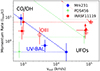 |
Fig. 13. Momentum rate vs. outflow velocity of different outflow phases for three well-known targets. Red symbols refer to IRASF11119: filled circles are taken from Nardini & Zubovas (2018). The empty diamond shows the UFOH momentum rate derived from the XSTAR fit, while the empty star shows the results from the DISK-WIND fit. The empty pentagon shows the momentum rate of the large-scale ionized outflow observed in [OIII]. Blue squares refer to Mrk231 (Feruglio et al. 2015) and green triangles to PDS456 (Bischetti et al. 2019). Data points at vout ∼ 103 km s−1 refer to molecular outflows detected in CO or OH. Data points at intermediate velocities (3 − 5000 km s−1) refer to OIII and UV winds, while at vout > 104 km s−1 refer to UFOs. Dotted horizontal lines show the expected evolution of a momentum-driven outflow, while dashed lines show the momentum boost expected for an energy-driven outflow. |
We compare our target with two local QSOs/ULIRGS systems, Mrk231 and PDS456, chosen as two of the best-studied multiphase outflows and at the two extremes of the wind propagation mechanisms: PDS456 also known as “the gentle monster” (Bischetti et al. 2019), has a large scale outflow detected in CO(3-2) with ALMA, with a momentum flux much smaller than the one measured from the very well studied and persistent X-ray UFO (e.g. Nardini et al. 2015; Matzeu et al. 2016). Mrk231, on the other hand, exhibits a powerful kpc-scale, multiphase (molecular and highly ionized, UV-BAL) outflow consistent with an energy-driven expansion powered by the nuclear wind observed in the X-rays (Feruglio et al. 2015).
These two sources are at the two extremes of the broad range of momentum boosts observed in the increasing sample of sources from which the energetics of the different outflow phases have been derived. In general, they show behaviors following either the momentum- or the energy-driven framework, with a majority in the first group (Tozzi et al. 2021; Bonanomi et al. 2023).
IRASF11119 is one of the very few sources for which the energetics of the large-scale outflow have been derived both in the molecular and ionized phases. According to the values derived in this work from the analysis of the new X-ray observations, the momentum flux of the nuclear UFO is very high in terms of Lbol/c, Ṗout ≳ 1 Lbol/c from the XSTAR fit or Ṗout ∼ 6 Lbol/c from the DISK-WIND results, while the momentum fluxes of the large-scale outflows are comparable with what observed in Mrk231 (Ṗout = 1 − 10 Lbol/c). The source, therefore, falls in the predominant group of sources (see Smith et al. 2019; Bonanomi et al. 2023) for which the large-scale wind appears to be not significantly boosted with respect to the nuclear outflow.
This could be due to the fact that the flow remains momentum-driven even at large distances from the SMBH, despite the expectations that beyond a few 100s pc the Compton cooling should become ineffective (e.g. King et al. 2011), or could be due to an inefficient coupling of the UFO with the host-galaxy ISM (Tombesi et al. 2015). Alternatively, the UFO observed today may be more powerful than it has been – on average – in the past few Myrs (flow time of the CO large scale outflow) so that the large scale outflow is the result of several short bursts of Eddington limited accretion episodes (see Nardini & Zubovas 2018; Zubovas & Nardini 2020). This is consistent with a chaotic feeding mechanism, as predicted by the CCA scenario (e.g.; Gaspari et al. 2017). Unfortunately, we do not have direct access to what has been the duty cycle of the wind over time scales of 105 − 106 years, i.e., the flow time of the OH and CO, respectively, as estimated from the ratio Rout/Vout in Veilleux et al. (2017).
On the other hand, a purely energy-driven expansion powered by a steady nuclear wind like the one observed in this work would imply large-scale momentum rates of hundreds to thousands times Lbol/c, i.e., mass outflow rates of more than several thousand M⊙/yr. Such extreme mass outflow rates have been observed only in the most powerful high-z systems, with typical Lbol > 1047 erg s−1 (Carniani et al. 2015; Bischetti et al. 2017) and in only a couple of extreme radio galaxies (Nesvadba et al. 2008) where the AGN Lbol is comparable to IRASF11119 (few×1046 erg s−1), but the outflow is most probably powered by the strong radio jets.
10. Summary
In this work, we have analyzed the new XMM-Newton and NuSTAR data collected for the highly accreting, post-merger ULIRG/QSO system IRASF11119, together with its SDSS optical spectrum. The results can be summarized as follows:
-
A “classical” nuclear wind with high column and ionization (UFOH), outflowing at vout ∼ 0.27c is clearly detected in the hard band, with parameters comparable to the previous Suzaku and NuSTAR observations, while a new component with lower column and ionization (UFOL) but similar speed is detected in the soft band.
-
We robustly measure one of the lowest high-energy cutoffs observed in AGN, Ecut ∼ 25 − 30 keV. Several other examples of sources with similar properties suggest that steep X-ray spectra – either soft power-laws or low cutoff – may promote or be connected with strong nuclear winds.
-
The optical spectrum shows a strong ionized large-scale outflow in the [OIII] forbidden lines, while several other forbidden lines are detected with decreasing outflow velocity for decreasing ionization potential, interpreted as an outflow decelerating, via entrainment, in a stratified medium, photoionized by the AGN.
-
The energetics derived for the UFOH, both from standard assumptions applied to the XSTAR fit and more directly from the DISK-WIND fit, are large, such that the mass outflow rate is comparable with the mass accretion rate and to the Eddington limit mass, Ṁout ∼ Ṁacc ∼ ṀEdd.
-
The absence of a significant momentum boost between the nuclear UFO and the different phases of the large-scale outflow suggests either a momentum-driven expansion of the wind, or a small coupling between the nuclear outflow and the ISM, or strong variability of the nuclear outflow power on time scales comparable with the large scale outflow flow-time (∼0.1 − 1 Myr).
Including IRASF11119 in the broader context of the SUBWAYS sample of z = 0.1 − 0.5 QSOs with comparable X-ray spectral quality gives a total UFO detection fraction of  (8 over 23 sources), slightly larger than the ∼30% derived in Matzeu et al. (2023) and identical to the value derived in the local Universe in Tombesi et al. (2010). This is without considering the well-known, persistent UFO detected in PDS 456, which would belong to the z = 0.1 − 0.5 sample but is an outlier in terms of BH mass and luminosity.
IRASF11119 will be a natural target for XRISM (XRISM Science Team 2020) observations: the high-resolution spectra of Resolve (Ishisaki et al. 2018) will allow to i) characterize the physical properties of the soft X-ray component of the UFO, which is now unresolved in a blend of multiple absorption lines probably from Ne and Fe ii) constrain with unprecedented accuracy the properties of the high energy UFO components by resolving individual Fe XXV/XXVI absorption lines iii) shed light on the launching mechanism if, as expected, the detailed shape of the absorption features are different for magnetic, radiation, and thermal driving (Fukumura et al. 2022).
The velocity is derived from the observed absorber redshift table parameter zo, using the Doppler formula and the relations between intrinsic absorber redshift za and source cosmological redshift zc described e.g., in Tombesi et al. (2011).
Acknowledgments
We thank the anonymous referee for their valuable feedback, which significantly enhanced the quality of this manuscript. GL, GAM, and MB acknowledge support and funding from Accordo Attuativo ASI-INAF n. 2017-14-H.0. GL, EB, MC and MD acknowledge support from PRIN MIUR 2017 Black Hole Winds and the Baryon Life Cycle of Galaxies, 2017PH3WAT. EB acknowledges the support of the INAF Large Grant 2022 “The metal circle: a new sharp view of the baryon cycle up to Cosmic Dawn with the latest generation IFU facilities”. FT acknowledges funding from the European Union – Next Generation EU, PRIN/MUR 2022 (2022K9N5B4). AL acknowledges support from the HORIZON-2020 grant “Integrated Activities for the High Energy Astrophysics Domain” (AHEAD-2020), G.A. 871158). JR and VB acknowledge support through NASA grant 80NSSC22K0474. MG acknowledges support from the ERC Consolidator Grant BlackHoleWeather (101086804). RS acknowledges support from the agreement ASI-INAF eXTP Fase B – 2020-3-HH.1-2021 and the INAF-PRIN grant “A Systematic Study of the largest reservoir of baryons and metals in the Universe: the circumgalactic medium of galaxies” (No. 1.05.01.85.10). MD gratefully acknowledges INAF funding through the “Ricerca Fondamentale 2022” program (mini-grant 1.05.12.04.04). MP acknowledges grant PID2021-127718NB-I00 funded by the Spanish Ministry of Science and Innovation/State Agency of Research (MICIN/AEI/ 10.13039/501100011033).
References
- An, H., Madsen, K. K., Westergaard, N. J., et al. 2014, SPIE Conf. Ser., 9144, 91441Q [NASA ADS] [Google Scholar]
- Arnaud, K. A. 1996, ASP Conf. Ser., 101, 17 [Google Scholar]
- Baloković, M., Harrison, F. A., Madejski, G., et al. 2020, ApJ, 905, 41 [Google Scholar]
- Baron, D., & Netzer, H. 2019, MNRAS, 486, 4290 [Google Scholar]
- Bautista, M. A., & Kallman, T. R. 2001, ApJS, 134, 139 [Google Scholar]
- Behar, E., Sako, M., & Kahn, S. M. 2001, ApJ, 563, 497 [NASA ADS] [CrossRef] [Google Scholar]
- Bertola, E., Dadina, M., Cappi, M., et al. 2020, A&A, 638, A136 [NASA ADS] [CrossRef] [EDP Sciences] [Google Scholar]
- Bertola, E., Vignali, C., Lanzuisi, G., et al. 2022, A&A, 662, A98 [NASA ADS] [CrossRef] [EDP Sciences] [Google Scholar]
- Bischetti, M., Piconcelli, E., Vietri, G., et al. 2017, A&A, 598, A122 [NASA ADS] [CrossRef] [EDP Sciences] [Google Scholar]
- Bischetti, M., Piconcelli, E., Feruglio, C., et al. 2019, A&A, 628, A118 [NASA ADS] [CrossRef] [EDP Sciences] [Google Scholar]
- Blustin, A. J., Page, M. J., Fuerst, S. V., Branduardi-Raymont, G., & Ashton, C. E. 2005, A&A, 431, 111 [CrossRef] [EDP Sciences] [Google Scholar]
- Bonanomi, F., Cicone, C., Severgnini, P., et al. 2023, A&A, 673, A46 [NASA ADS] [CrossRef] [EDP Sciences] [Google Scholar]
- Boroson, T. A., & Green, R. F. 1992, ApJS, 80, 109 [Google Scholar]
- Brusa, M., Bongiorno, A., Cresci, G., et al. 2015, MNRAS, 446, 2394 [NASA ADS] [CrossRef] [Google Scholar]
- Calzetti, D., Kinney, A. L., & Storchi-Bergmann, T. 1994, ApJ, 429, 582 [Google Scholar]
- Calzetti, D., Armus, L., Bohlin, R. C., et al. 2000, ApJ, 533, 682 [NASA ADS] [CrossRef] [Google Scholar]
- Cano-Díaz, M., Maiolino, R., Marconi, A., et al. 2012, A&A, 537, L8 [NASA ADS] [CrossRef] [EDP Sciences] [Google Scholar]
- Carniani, S., Marconi, A., Maiolino, R., et al. 2015, A&A, 580, A102 [NASA ADS] [CrossRef] [EDP Sciences] [Google Scholar]
- Cash, W. 1979, ApJ, 228, 939 [Google Scholar]
- Chartas, G., Brandt, W. N., Gallagher, S. C., & Garmire, G. P. 2002, ApJ, 579, 169 [Google Scholar]
- Chartas, G., Kochanek, C. S., Dai, X., Poindexter, S., & Garmire, G. 2009, ApJ, 693, 174 [Google Scholar]
- Chartas, G., Davidson, E., Brusa, M., et al. 2020, MNRAS, 496, 598 [Google Scholar]
- Chartas, G., Cappi, M., Vignali, C., et al. 2021, ApJ, 920, 24 [NASA ADS] [CrossRef] [Google Scholar]
- Chatzikos, M., Bianchi, S., Camilloni, F., et al. 2023, Rev. Mex. Astron. Astrofis., 59, 327 [Google Scholar]
- Condon, J. J., Cotton, W. D., Greisen, E. W., et al. 1998, AJ, 115, 1693 [Google Scholar]
- Costa, T., Sijacki, D., & Haehnelt, M. G. 2014, MNRAS, 444, 2355 [Google Scholar]
- Costantini, E., Kaastra, J. S., Arav, N., et al. 2007, A&A, 461, 121 [CrossRef] [EDP Sciences] [Google Scholar]
- Dauser, T., García, J., Parker, M. L., Fabian, A. C., & Wilms, J. 2014, MNRAS, 444, L100 [NASA ADS] [CrossRef] [Google Scholar]
- Davies, R., Baron, D., Shimizu, T., et al. 2020, MNRAS, 498, 4150 [Google Scholar]
- Di Gesu, L., Costantini, E., Arav, N., et al. 2013, A&A, 556, A94 [NASA ADS] [CrossRef] [EDP Sciences] [Google Scholar]
- Ding, Y., Li, R., Ho, L. C., & Ricci, C. 2022, ApJ, 931, 77 [NASA ADS] [CrossRef] [Google Scholar]
- Duras, F., Bongiorno, A., Ricci, F., et al. 2020, A&A, 636, A73 [NASA ADS] [CrossRef] [EDP Sciences] [Google Scholar]
- Eracleous, M., & Halpern, J. P. 2004, ApJS, 150, 181 [NASA ADS] [CrossRef] [Google Scholar]
- Fabian, A. C. 2012, ARA&A, 50, 455 [Google Scholar]
- Fabian, A. C., Lohfink, A., Kara, E., et al. 2015, MNRAS, 451, 4375 [Google Scholar]
- Faucher-Giguère, C.-A., & Quataert, E. 2012, MNRAS, 425, 605 [Google Scholar]
- Feruglio, C., Fiore, F., Carniani, S., et al. 2015, A&A, 583, A99 [NASA ADS] [CrossRef] [EDP Sciences] [Google Scholar]
- Feruglio, C., Ferrara, A., Bischetti, M., et al. 2017, A&A, 608, A30 [NASA ADS] [CrossRef] [EDP Sciences] [Google Scholar]
- Fiore, F., Feruglio, C., Shankar, F., et al. 2017, A&A, 601, A143 [NASA ADS] [CrossRef] [EDP Sciences] [Google Scholar]
- Fukumura, K., Dadina, M., Matzeu, G., et al. 2022, ApJ, 940, 6 [NASA ADS] [CrossRef] [Google Scholar]
- García, J., Dauser, T., Lohfink, A., et al. 2014, ApJ, 782, 76 [Google Scholar]
- Gaspari, M., & Sądowski, A. 2017, ApJ, 837, 149 [NASA ADS] [CrossRef] [Google Scholar]
- Gaspari, M., Brighenti, F., & Temi, P. 2012, MNRAS, 424, 190 [NASA ADS] [CrossRef] [Google Scholar]
- Gaspari, M., Temi, P., & Brighenti, F. 2017, MNRAS, 466, 677 [Google Scholar]
- Gaspari, M., Tombesi, F., & Cappi, M. 2020, Nat. Astron., 4, 10 [Google Scholar]
- Gianolli, V. E., Bianchi, S., Petrucci, P.-O., et al. 2024, A&A, 687, A235 [NASA ADS] [CrossRef] [EDP Sciences] [Google Scholar]
- Gofford, J., Reeves, J. N., Tombesi, F., et al. 2013, MNRAS, 430, 60 [Google Scholar]
- Guo, H., Shen, Y., & Wang, S. 2018, Astrophysics Source Code Library [record ascl:1809.008] [Google Scholar]
- Gupta, A., Mathur, S., Krongold, Y., & Nicastro, F. 2013a, ApJ, 768, 141 [NASA ADS] [CrossRef] [Google Scholar]
- Gupta, A., Mathur, S., Krongold, Y., & Nicastro, F. 2013b, ApJ, 772, 66 [NASA ADS] [CrossRef] [Google Scholar]
- Gupta, A., Mathur, S., & Krongold, Y. 2015, ApJ, 798, 4 [Google Scholar]
- Harrison, F. A., Craig, W. W., Christensen, F. E., et al. 2013, ApJ, 770, 103 [Google Scholar]
- Harrison, C. M., Costa, T., Tadhunter, C. N., et al. 2018, Nat. Astron., 2, 198 [Google Scholar]
- Hasinger, G., Schartel, N., & Komossa, S. 2002, ApJ, 573, L77 [Google Scholar]
- HI4PI Collaboration (Ben Bekhti, N., et al.) 2016, A&A, 594, A116 [NASA ADS] [CrossRef] [EDP Sciences] [Google Scholar]
- Hinkle, J. T., & Mushotzky, R. 2021, MNRAS, 506, 4960 [NASA ADS] [CrossRef] [Google Scholar]
- Hu, C., Wang, J.-M., Ho, L. C., et al. 2008, ApJ, 683, L115 [NASA ADS] [CrossRef] [Google Scholar]
- Igo, Z., Parker, M. L., Matzeu, G. A., et al. 2020, MNRAS, 493, 1088 [NASA ADS] [CrossRef] [Google Scholar]
- Ishisaki, Y., Ezoe, Y., Yamada, S., et al. 2018, J. Low Temp. Phys., 193, 991 [NASA ADS] [CrossRef] [Google Scholar]
- Jiang, J., Parker, M. L., Fabian, A. C., et al. 2018, MNRAS, 477, 3711 [NASA ADS] [CrossRef] [Google Scholar]
- Kaastra, J. S., & Bleeker, J. A. M. 2016, A&A, 587, A151 [NASA ADS] [CrossRef] [EDP Sciences] [Google Scholar]
- Kaastra, J. S., Petrucci, P. O., Cappi, M., et al. 2011, A&A, 534, A36 [NASA ADS] [CrossRef] [EDP Sciences] [Google Scholar]
- Kaastra, J. S., Detmers, R. G., Mehdipour, M., et al. 2012, A&A, 539, A117 [NASA ADS] [CrossRef] [EDP Sciences] [Google Scholar]
- Kaastra, J. S., Kriss, G. A., Cappi, M., et al. 2014, Science, 345, 64 [Google Scholar]
- Kallman, T. R., Palmeri, P., Bautista, M. A., Mendoza, C., & Krolik, J. H. 2004, ApJS, 155, 675 [Google Scholar]
- Kammoun, E. S., Risaliti, G., Stern, D., et al. 2017, MNRAS, 465, 1665 [CrossRef] [Google Scholar]
- Kammoun, E. S., Igo, Z., Miller, J. M., et al. 2023, MNRAS, 522, 5217 [NASA ADS] [CrossRef] [Google Scholar]
- Kamraj, N., Harrison, F. A., Baloković, M., Lohfink, A., & Brightman, M. 2018, ApJ, 866, 124 [CrossRef] [Google Scholar]
- Kamraj, N., Brightman, M., Harrison, F. A., et al. 2022, ApJ, 927, 42 [NASA ADS] [CrossRef] [Google Scholar]
- Kang, J.-L., & Wang, J.-X. 2022, ApJ, 929, 141 [NASA ADS] [CrossRef] [Google Scholar]
- Kang, J. L., & Wang, J. X. 2023, ArXiv e-prints [arXiv:2311.15499] [Google Scholar]
- Kara, E., García, J. A., Lohfink, A., et al. 2017, MNRAS, 468, 3489 [NASA ADS] [CrossRef] [Google Scholar]
- King, A., & Pounds, K. 2015, ARA&A, 53, 115 [NASA ADS] [CrossRef] [Google Scholar]
- King, A. R., Zubovas, K., & Power, C. 2011, MNRAS, 415, L6 [NASA ADS] [CrossRef] [Google Scholar]
- Kobayashi, H., Ohsuga, K., Takahashi, H. R., et al. 2018, PASJ, 70, 22 [NASA ADS] [Google Scholar]
- Komossa, S., Voges, W., Xu, D., et al. 2006, AJ, 132, 531 [NASA ADS] [CrossRef] [Google Scholar]
- Komossa, S., Xu, D., Zhou, H., Storchi-Bergmann, T., & Binette, L. 2008, ApJ, 680, 926 [NASA ADS] [CrossRef] [Google Scholar]
- Krolik, J. H., & Kriss, G. A. 2001, ApJ, 561, 684 [CrossRef] [Google Scholar]
- Krongold, Y., Nicastro, F., Elvis, M., et al. 2007, ApJ, 659, 1022 [NASA ADS] [CrossRef] [Google Scholar]
- Krongold, Y., Longinotti, A. L., Santos-Lleó, M., et al. 2021, ApJ, 917, 39 [NASA ADS] [CrossRef] [Google Scholar]
- Kubota, A., & Done, C. 2019, MNRAS, 489, 524 [NASA ADS] [CrossRef] [Google Scholar]
- Laha, S., Reynolds, C. S., Reeves, J., et al. 2021, Nat. Astron., 5, 13 [NASA ADS] [CrossRef] [Google Scholar]
- Lanzuisi, G., Giustini, M., Cappi, M., et al. 2012, A&A, 544, A2 [NASA ADS] [CrossRef] [EDP Sciences] [Google Scholar]
- Lanzuisi, G., Gilli, R., Cappi, M., et al. 2019, ApJ, 875, L20 [Google Scholar]
- Laurenti, M., Luminari, A., Tombesi, F., et al. 2021, A&A, 645, A118 [NASA ADS] [CrossRef] [EDP Sciences] [Google Scholar]
- Lípari, S., Terlevich, R., Díaz, R. J., et al. 2003, MNRAS, 340, 289 [CrossRef] [Google Scholar]
- Longinotti, A. L., Krongold, Y., Guainazzi, M., et al. 2015, ApJ, 813, L39 [Google Scholar]
- Luminari, A., Tombesi, F., Piconcelli, E., et al. 2020, A&A, 633, A55 [NASA ADS] [CrossRef] [EDP Sciences] [Google Scholar]
- Luminari, A., Nicastro, F., Elvis, M., et al. 2021, A&A, 646, A111 [NASA ADS] [CrossRef] [EDP Sciences] [Google Scholar]
- Luminari, A., Marinucci, A., Bianchi, S., et al. 2023, ApJ, 950, 160 [NASA ADS] [CrossRef] [Google Scholar]
- Lutz, D., Sturm, E., Janssen, A., et al. 2020, A&A, 633, A134 [NASA ADS] [CrossRef] [EDP Sciences] [Google Scholar]
- Magorrian, J., Tremaine, S., Richstone, D., et al. 1998, AJ, 115, 2285 [Google Scholar]
- Maiolino, R., Gallerani, S., Neri, R., et al. 2012, MNRAS, 425, L66 [Google Scholar]
- Marasco, A., Cresci, G., Nardini, E., et al. 2020, A&A, 644, A15 [EDP Sciences] [Google Scholar]
- Marconi, A., Risaliti, G., Gilli, R., et al. 2004, MNRAS, 351, 169 [Google Scholar]
- Marinucci, A., Vietri, G., Piconcelli, E., et al. 2022, A&A, 666, A169 [NASA ADS] [CrossRef] [EDP Sciences] [Google Scholar]
- Markowitz, A., Reeves, J. N., & Braito, V. 2006, ApJ, 646, 783 [NASA ADS] [CrossRef] [Google Scholar]
- Marziani, P., Zamanov, R. K., Sulentic, J. W., & Calvani, M. 2003, MNRAS, 345, 1133 [NASA ADS] [CrossRef] [Google Scholar]
- Marziani, P., Sulentic, J. W., Stirpe, G. M., et al. 2016, Ap&SS, 361, 3 [NASA ADS] [CrossRef] [Google Scholar]
- Matzeu, G. A., Reeves, J. N., Nardini, E., et al. 2016, MNRAS, 458, 1311 [Google Scholar]
- Matzeu, G. A., Lieu, M., Costa, M. T., et al. 2022, MNRAS, 515, 6172 [NASA ADS] [CrossRef] [Google Scholar]
- Matzeu, G. A., Brusa, M., Lanzuisi, G., et al. 2023, A&A, 670, A182 [Google Scholar]
- McKernan, B., Yaqoob, T., & Reynolds, C. S. 2007, MNRAS, 379, 1359 [NASA ADS] [CrossRef] [Google Scholar]
- Medhipour, M., Kriss, G. A., Krongold, Y., et al. 2023, A&A, 670, A183 [NASA ADS] [CrossRef] [EDP Sciences] [Google Scholar]
- Miniutti, G., & Fabian, A. C. 2006, MNRAS, 366, 115 [NASA ADS] [Google Scholar]
- Nardini, E., & Zubovas, K. 2018, MNRAS, 478, 2274 [Google Scholar]
- Nardini, E., Reeves, J. N., Gofford, J., et al. 2015, Science, 347, 860 [Google Scholar]
- Nardini, E., Lusso, E., & Bisogni, S. 2019, MNRAS, 482, L134 [Google Scholar]
- Nesvadba, N. P. H., Lehnert, M. D., De Breuck, C., Gilbert, A. M., & van Breugel, W. 2008, A&A, 491, 407 [NASA ADS] [CrossRef] [EDP Sciences] [Google Scholar]
- Nomura, M., Ohsuga, K., & Done, C. 2020, MNRAS, 494, 3616 [NASA ADS] [CrossRef] [Google Scholar]
- Osterbrock, D. E. 1989, Astrophysics of Gaseous Nebulae and Active Galactic Nuclei (University Science Books) [Google Scholar]
- Pan, X., Zhou, H., Liu, W., et al. 2019, ApJ, 883, 173 [NASA ADS] [CrossRef] [Google Scholar]
- Parker, M. L., Alston, W. N., Buisson, D. J. K., et al. 2017, MNRAS, 469, 1553 [NASA ADS] [CrossRef] [Google Scholar]
- Parker, M. L., Matzeu, G. A., Guainazzi, M., et al. 2018, MNRAS, 480, 2365 [NASA ADS] [CrossRef] [Google Scholar]
- Perna, M., Brusa, M., Cresci, G., et al. 2015, A&A, 574, A82 [NASA ADS] [CrossRef] [EDP Sciences] [Google Scholar]
- Piconcelli, E., Jimenez-Bailón, E., Guainazzi, M., et al. 2004, MNRAS, 351, 161 [Google Scholar]
- Piconcelli, E., Jimenez-Bailón, E., Guainazzi, M., et al. 2005, A&A, 432, 15 [NASA ADS] [CrossRef] [EDP Sciences] [Google Scholar]
- Porquet, D., Reeves, J. N., Uttley, P., & Turner, T. J. 2004, A&A, 427, 101 [NASA ADS] [CrossRef] [EDP Sciences] [Google Scholar]
- Pounds, K. A., & Vaughan, S. 2011, MNRAS, 415, 2379 [NASA ADS] [CrossRef] [Google Scholar]
- Pounds, K. A., Reeves, J. N., King, A. R., et al. 2003, MNRAS, 345, 705 [Google Scholar]
- Pounds, K. A., Lobban, A., Reeves, J. N., Vaughan, S., & Costa, M. 2016, MNRAS, 459, 4389 [Google Scholar]
- Proga, D., & Kallman, T. R. 2004, ApJ, 616, 688 [Google Scholar]
- Protassov, R., van Dyk, D. A., Connors, A., Kashyap, V. L., & Siemiginowska, A. 2002, ApJ, 571, 545 [NASA ADS] [CrossRef] [Google Scholar]
- Reeves, J. N., & Braito, V. 2019, ApJ, 884, 80 [NASA ADS] [CrossRef] [Google Scholar]
- Reeves, J. N., O’Brien, P. T., & Ward, M. J. 2003, ApJ, 593, L65 [Google Scholar]
- Reeves, J. N., Braito, V., Nardini, E., et al. 2016, ApJ, 824, 20 [NASA ADS] [CrossRef] [Google Scholar]
- Reeves, J. N., Braito, V., Nardini, E., et al. 2018a, ApJ, 854, L8 [NASA ADS] [CrossRef] [Google Scholar]
- Reeves, J. N., Lobban, A., & Pounds, K. A. 2018b, ApJ, 854, 28 [Google Scholar]
- Reeves, J. N., Braito, V., Chartas, G., et al. 2020, ApJ, 895, 37 [Google Scholar]
- Reeves, J. N., Braito, V., Porquet, D., et al. 2021, MNRAS, 500, 1974 [Google Scholar]
- Reynolds, C. S. 1997, MNRAS, 286, 513 [NASA ADS] [CrossRef] [Google Scholar]
- Ricci, C., Ho, L. C., Fabian, A. C., et al. 2018, MNRAS, 480, 1819 [NASA ADS] [CrossRef] [Google Scholar]
- Rose, M., Tadhunter, C., Ramos Almeida, C., et al. 2018, MNRAS, 474, 128 [Google Scholar]
- Rupke, D. S., Veilleux, S., & Sanders, D. B. 2005, ApJ, 632, 751 [NASA ADS] [CrossRef] [Google Scholar]
- Sądowski, A., & Narayan, R. 2016, MNRAS, 456, 3929 [CrossRef] [Google Scholar]
- Saez, C., & Chartas, G. 2011, ApJ, 737, 91 [NASA ADS] [CrossRef] [Google Scholar]
- Sako, M., Kahn, S. M., Behar, E., et al. 2001, A&A, 365, L168 [NASA ADS] [CrossRef] [EDP Sciences] [Google Scholar]
- Schlegel, D. J., Finkbeiner, D. P., & Davis, M. 1998, ApJ, 500, 525 [Google Scholar]
- Serafinelli, R., & De Rosa, A. 2024, A&A, in press, https://doi.org/10.1051/0004-6361/202450777 [Google Scholar]
- Serafinelli, R., Tombesi, F., Vagnetti, F., et al. 2019, A&A, 627, A121 [NASA ADS] [CrossRef] [EDP Sciences] [Google Scholar]
- Silk, J., & Rees, M. J. 1998, A&A, 331, L1 [NASA ADS] [Google Scholar]
- Sim, S. A., Long, K. S., Miller, L., & Turner, T. J. 2008, MNRAS, 388, 611 [CrossRef] [Google Scholar]
- Sim, S. A., Miller, L., Long, K. S., Turner, T. J., & Reeves, J. N. 2010, MNRAS, 404, 1369 [NASA ADS] [Google Scholar]
- Smith, R. N., Tombesi, F., Veilleux, S., Lohfink, A. M., & Luminari, A. 2019, ApJ, 887, 69 [NASA ADS] [CrossRef] [Google Scholar]
- Spoon, H. W. W., & Holt, J. 2009, ApJ, 702, L42 [NASA ADS] [CrossRef] [Google Scholar]
- Strüder, L., Briel, U., Dennerl, K., et al. 2001, A&A, 365, L18 [Google Scholar]
- Takeuchi, S., Ohsuga, K., & Mineshige, S. 2013, PASJ, 65, 88 [Google Scholar]
- Tananbaum, H., Avni, Y., Branduardi, G., et al. 1979, ApJ, 234, L9 [Google Scholar]
- Tombesi, F., Cappi, M., Reeves, J. N., et al. 2010, A&A, 521, A57 [NASA ADS] [CrossRef] [EDP Sciences] [Google Scholar]
- Tombesi, F., Cappi, M., Reeves, J. N., et al. 2011, ApJ, 742, 44 [Google Scholar]
- Tombesi, F., Cappi, M., Reeves, J. N., & Braito, V. 2012, MNRAS, 422, L1 [Google Scholar]
- Tombesi, F., Cappi, M., Reeves, J. N., et al. 2013, MNRAS, 430, 1102 [Google Scholar]
- Tombesi, F., Tazaki, F., Mushotzky, R. F., et al. 2014, MNRAS, 443, 2154 [NASA ADS] [CrossRef] [Google Scholar]
- Tombesi, F., Meléndez, M., Veilleux, S., et al. 2015, Nature, 519, 436 [NASA ADS] [CrossRef] [Google Scholar]
- Tombesi, F., Veilleux, S., Meléndez, M., et al. 2017, ApJ, 850, 151 [Google Scholar]
- Tortosa, A., Bianchi, S., Marinucci, A., Matt, G., & Petrucci, P. O. 2018, A&A, 614, A37 [NASA ADS] [CrossRef] [EDP Sciences] [Google Scholar]
- Tortosa, A., Ricci, C., Tombesi, F., et al. 2022, MNRAS, 509, 3599 [Google Scholar]
- Tortosa, A., Ricci, C., Ho, L. C., et al. 2023, MNRAS, 519, 6267 [NASA ADS] [CrossRef] [Google Scholar]
- Tortosa, A., Zappacosta, L., Piconcelli, E., et al. 2024, A&A, submitted [Google Scholar]
- Tozzi, G., Cresci, G., Marasco, A., et al. 2021, A&A, 648, A99 [NASA ADS] [CrossRef] [EDP Sciences] [Google Scholar]
- Turner, M. J. L., Abbey, A., Arnaud, M., et al. 2001, A&A, 365, L27 [CrossRef] [EDP Sciences] [Google Scholar]
- Veilleux, S. 1991, ApJ, 368, 158 [NASA ADS] [CrossRef] [Google Scholar]
- Veilleux, S., Bolatto, A., Tombesi, F., et al. 2017, ApJ, 843, 18 [Google Scholar]
- Veilleux, S., Meléndez, M., Sturm, E., et al. 2013, ApJ, 776, 27 [Google Scholar]
- Veilleux, S., Maiolino, R., Bolatto, A. D., & Aalto, S. 2020, A&A Rev., 28, 2 [NASA ADS] [CrossRef] [Google Scholar]
- Wachter, K., Leach, R., & Kellogg, E. 1979, ApJ, 230, 274 [NASA ADS] [CrossRef] [Google Scholar]
- Wang, J. X., Wang, T. G., Tozzi, P., et al. 2005, ApJ, 631, L33 [NASA ADS] [CrossRef] [Google Scholar]
- Wittor, D., & Gaspari, M. 2020, MNRAS, 498, 4983 [NASA ADS] [CrossRef] [Google Scholar]
- XRISM Science Team 2020, Science with the X-ray Imaging and Spectroscopy Mission (XRISM) [Google Scholar]
- Yang, J., Paragi, Z., An, T., et al. 2020, MNRAS, 494, 1744 [NASA ADS] [CrossRef] [Google Scholar]
- Yaqoob, T., George, I. M., Nandra, K., et al. 1999, ApJ, 525, L9 [NASA ADS] [CrossRef] [Google Scholar]
- Zamanov, R., Marziani, P., Sulentic, J. W., et al. 2002, ApJ, 576, L9 [NASA ADS] [CrossRef] [Google Scholar]
- Zappacosta, L., Piconcelli, E., Fiore, F., et al. 2023, A&A, 678, A201 [NASA ADS] [CrossRef] [EDP Sciences] [Google Scholar]
- Zheng, Z. Y., & Wang, J. X. 2008, ApJ, 688, 116 [NASA ADS] [CrossRef] [Google Scholar]
- Zheng, X. Z., Xia, X. Y., Mao, S., Wu, H., & Deng, Z. G. 2002, AJ, 124, 18 [NASA ADS] [CrossRef] [Google Scholar]
- Zubovas, K., & King, A. 2012, ApJ, 745, L34 [Google Scholar]
- Zubovas, K., & Nardini, E. 2020, MNRAS, 498, 3633 [Google Scholar]
Appendix A: 1-4 keV Spectral Scan
In Figure A.1, we report the results of the line scan performed in the intermediate energy range (1.5-4 keV) where MgII, Si XIV, and SXVI Lyα absorption lines produced by UFOs are sometimes observed, even in CCD-resolution spectra (e.g., Pounds et al. 2003; Parker et al. 2018). The continuum is the same as described in Sect. 4.1 while the details of the scan are the same as described in Sect. 4.2. Indeed, three narrow residuals can be seen at energies roughly corresponding to the expected energies of such lines for an outflow velocity of vout = 0.27c (dashed lines in Figure A.1). The significance of these features is, however, low and up to 99% confidence level only for the S XVI Lyα line. The Δ𝒞 values from the fit with a Gaussian line for each of these features are 4.27, 3.17, and 8.44, respectively. They contribute, nonetheless, to the total Δ𝒞 when the XSTAR or DISK-WIND tables are added to the continuum. As a consequence, including these complex absorption templates into the fit results in a significantly increased statistical significance compared to the fit with the single Gaussian lines (see Sect. 6.1).
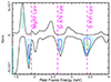 |
Fig. A.1. Confidence contours showing deviations from the continuum model described in Sect. 4.1 in the intermediate band. Contours as in Figure 2. |
Appendix B: MonteCarlo simulations
For our null hypothesis baseline model, we used the 0.6 − 24 keV rest frame best-fit continuum model described in Sect. 4.1. We simulated 1000 sets of XMM-Newton and NuSTAR spectra with the same response matrices, exposure times, and background levels as the read data. These spectra were binned following the same 𝒦ℬ binning used for the observed spectra. We then fitted the continuum model to each set of simulated spectra, leaving the same free parameters described in Sect. 4.1. Then, we simulated the spectra again, starting from the new best-fit values to accommodate for random continuum variations. We fitted these newly generated spectra again to find the new continuum best-ft (see Matzeu et al. 2023 for a similar procedure).
We perform a second fit on the same set of simulated spectra, adding a narrow Gaussian profile, with line width fixed to zero and normalization set to zero but free to fluctuate between negative and positive values to probe both absorption and emission features. The rest-frame Gaussian line energy is then stepped with the STEPPAR command in XSPEC, between 0.5 and 2 keV in ΔE = 15 eV for the soft band features (Em1 and Abs1) and between 5 and 10 keV in ΔE = 25 eV for the hard band features (Em2,3 and Abs2,3) to find the global 𝒞−stat minimum for each set of spectra in the respective energy ranges. We verified that extending the hard band range to, e.g., 12 keV to take into account that Abs3 is observed above 10 keV would not change the ℳ𝒞 results, as the strongest random fluctuations always occur where the count statistic is larger, i.e., toward the low energy boundary, between ∼5 and ∼7 keV. Interestingly, this also implies that by performing the search on the full 4-10 keV band - as usually done in the literature - we tend to underestimate the significance of the UFO features, as by definition, they appear above ∼7.5 keV (see also Nardini et al. 2019).
This process maps the Δ𝒞 variations due to random fluctuations in the simulated spectra. The ℳ𝒞 statistical significance (Pℳ𝒞) of the emission/absorption line detections can be then computed as  where N is the number of simulated spectra showing a random fluctuation larger than the one observed in the data and S the number of simulations.
None of the realizations in the soft band show Δ𝒞 > 37.96 and therefore Em1 has Pℳ𝒞 > 99.9%, while 2 realizations have Δ𝒞 > 18.56, indicating Pℳ𝒞 = 99.8% for Abs1. None of the realizations in the hard band show Δ𝒞 > 22.28 and therefore Em2,3 and Abs2 all have Pℳ𝒞 > 99.9% while 2 exceed Δ𝒞 = 16.59 and therefore Abs3 has Pℳ𝒞 = 99.8%. Even the less prominent absorption features, Abs1 in the soft band and Abs3 at 11 keV, are significant at > 3σ from ℳ𝒞 simulations.
Having performed 1000 sets of simulations for the soft and hard band, respectively, the accuracy of Pℳ𝒞 is limited to the level of 1/1000. However, significantly increasing the number of trials to increase the accuracy of Pℳ𝒞 is computationally prohibitive due to the quite complex baseline model, the simultaneous fit of five different spectra, and the need to sample two different energy ranges.
Appendix C: Tests on Ecut measurements
For the spectral fits performed in this work, we used the 𝒦ℬ binning that optimizes the bin size based on the spectral resolution and the source counts available per resolution element, with the main goal of characterizing the emission and absorption features observed. However, to our knowledge, this binning scheme has never been tested for continuum parameters accuracy, with the recent exception of Zappacosta et al. (2023) where, however, it was tested in a completely different regime: extreme low counts statistic and simple power-law models.
We, therefore, tested the impact of different fit statistics and spectral binning on the continuum parameters Γ and Ecut with particular emphasis on the extremely low high energy cutoff found in section 7. We computed the Γ vs. Ecut contours for the 𝒞−stat fit on XMM-Newton, and NuSTAR spectra binned to 5 counts per bin, and for χ2 fits on spectra binned to 20 and 50 counts per bin. As can be seen in Figure B.1, the results are stable, independently of the binning scheme and statistics adopted for the fit. We also tested the impact of including the energy ranges 20-30 keV and 20-50 keV, where the NuSTAR spectra are background-dominated but where some source signal is still present. Once again, the results are stable, with Ecut in the range 25 − 30 ± 10 as for the fit limited to 20 keV observer-frame.
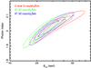 |
Fig. B.1. Contour plots of high energy cutoff vs. photon index for different binning schemes and statistics adopted. In red, the results from a fit performed with 𝒞−stat on spectra binned to 5 counts per bin, and in blue (green) from a fit performed with χ2 on spectra binned to 20 (50) counts per bin. |
Finally, we tested a posteriori the impact of the empirical correction of the EPIC effective area introduced in a 2022 EPIC calibration Technical Note5 to improve the cross-calibration in the hard band (∼6 − 10 keV) between XMM-Newton and NuSTAR. The updated ARF calibration - which translates into an increase by a factor up to 8% in the 9-10 keV band - has the effect of reducing the discrepancies between XMM-Newton and NuSTAR photon index and Ecut, in particular yielding slightly higher Γ and Ecut values in the joint fits of XMM-Newton and NuSTAR spectra of a sample of local AGN (Kang & Wang 2023). We, therefore, re-extracted the EPIC spectra with the newest calibration files and the parameter applyabsfluxcorr set to yes in the arfgen tool and recomputed the best-fit values for the different models described in 4. Given the data quality available for our target and its complex spectral shape, however, the small differences in the EPIC responses do not significantly affect our results, and the updated best-fit values are fully consistent within the error bars, with the results reported in the main text.
All Tables
Best-fit parameters and significance of the Gaussian emission and absorption lines.
Best-fit parameters of the model where a DISK-WIND grid was used to replace the XSTAR table to model the UFOH features.
All Figures
|
Fig. 1. XMM-Newton and NuSTAR spectra and continuum models and their residuals. a: background subtracted XMM-Newton (pn in black, MOS1+2 in red) and NuSTAR (FPMA+B in blue) spectra, and their corresponding background levels (gray, orange, and violet, respectively) are shown with the baseline continuum model (see Sect. 4.1). The MOS1 and 2 and FPM-A and -B spectra have been merged for plotting purposes. b: residuals (data-model/error), with respect to the baseline continuum model. In green, we highlight the energy ranges where the most prominent positive and negative residuals are found (see Sect. 4.2). c: residuals after including three emissions and three absorption Gaussian features (see Sect. 5). d: residuals after including two XSTAR tables to model the soft and hard band absorption features (see Sect. 6.1). |
| In the text | |
|
Fig. 2. Zoom in the soft (left) and hard (right) band of the residuals from panel b of Figure 1. The spectra in the right panel have been rebinned for clarity. Colors as in Figure 1. |
| In the text | |
|
Fig. 3. Confidence contours showing deviations from the continuum model described in Sect. 4.1 in the soft (left) and hard (right) band. Black contours show Δ𝒞 = +0.5 while the colored contours show Δ𝒞 = −2.3 (cyan), −4.61 (blue), −9.21 (green), −13.82 (red), −18.42 (magenta), corresponding to a significance of 68%, 90%, 99%, 99.9%, and 99.99% for two parameters. In both panels, the main transitions from ionized Ne and Fe are labeled at their rest-frame energies. |
| In the text | |
|
Fig. 4. Left: confidence contour levels of the column density NH and the ionization parameter log(ξ/erg cm s−1), for the best-fit model with two XSTAR tables, one with vturb = 1000 km s−1 for the low-ionization table UFOL and one with vturb = 3000 km s−1 for the high-ionization UFOH one. Right: contour plot of the outflow velocity for the UFOH in red and for UFOL in green. The blue lines mark one parameter’s 90, 99, and 99.9% confidence levels. |
| In the text | |
|
Fig. 5. Unfolded best-fit model (black) in νF(ν) including three XSTAR absorption tables. The emission lines are shown in magenta, and the scattered emission is in orange. The main absorption features due to the WA, UFOL, and UFOH are labeled in red, green, and blue, respectively. The ions producing the most prominent features are labeled in black. |
| In the text | |
|
Fig. 6. log(NH) vs. vout (left) and log(ξ) vs. vout (right) for the WA, UFOL, and UFOH components of IRASF11119 (red diamonds). The known soft-band detected fast winds from the literature are shown with colored points: light green (Gupta et al. 2013b); cyan (Gupta et al. 2015); sky blue (Longinotti et al. 2015); magenta (Reeves et al. 2016); blue (Pounds et al. 2016); orange (Jiang et al. 2018); yellow (Serafinelli et al. 2019); dark green (Krongold et al. 2021). The low-velocity WAs region (green), UFOs region (cyan), and the correlation fits linking low-velocity WAs and UFOs (dashed black lines) are derived from Tombesi et al. (2013). |
| In the text | |
|
Fig. 7. XMM-Newton and NuSTAR spectra with the best-fit continuum model and residuals, for the model described in Sect. 6.2, where the DISK-WIND table replaces the UFOH XSTAR table. The colors are the same as in Figure 1. |
| In the text | |
|
Fig. 8. Confidence contour levels of the DISK-WIND parameters fv vs. μ (left) and |
| In the text | |
|
Fig. 9. Confidence contour levels of the high energy cutoff vs. the photon index. The colored contours refer to the best-fit model with two UFO XSTAR absorption tables, described in Sect. 6.1, while the gray contours show the results from the continuum model only, described in Sect. 4.1. |
| In the text | |
|
Fig. 10. High-energy cutoff vs. intrinsic luminosity for local Seyferts measured with NuSTAR (gray dots, from the updated sample of Bertola et al. 2022), and the binned results from the BAT-selected sample (magenta downward pointing triangles, Ricci et al. 2018). Green data points show results for luminous quasars at z ≳ 0.5: pentagon from Kammoun et al. (2017); squares Lanzuisi et al. (2019); star Bertola et al. (2022); plus Marinucci et al. (2022); right-ward triangle Kammoun et al. (2023). PDS456 (Reeves et al. 2021) is shown in cyan and IRASF11119 in red. The different intrinsic luminosities obtained from the XSTAR and DISK-WIND fits are shown by the vertical error bar. The yellow/orange areas show the runaway pair-production forbidden region (Fabian et al. 2015; Lanzuisi et al. 2019) for different geometries and BH masses. |
| In the text | |
|
Fig. 11. Hβ, [OIII], and Hα regions of the optical spectrum of IRASF11119. The observed spectrum is plotted in gray, while the best fit is shown as the black dashed line. Different model components are traced by lines of different colors, as indicated by the label. The vertical dashed lines indicate the rest-frame wavelength for each labeled emission line, for z = 0.187. In the bottom panels, residuals are plotted. Note that the Hα shows significant residuals, possibly due to the blending with the [NII] doublet, but this effect is negligible for our goals. |
| In the text | |
|
Fig. 12. Distance from the ionizing source vs. velocity offset for different emission lines (labeled) modeled in the SDSS spectrum. The distance is derived from the ionization level at which each ion has the peak of relative abundance. The red curve is a power-law fit of the form vout = a × rb + c with the best-fit slope b = 0.20 ± 0.07. The gray dashed line shows a curve with a slope fixed to b = 0.5, the value for a simple ballistic trajectory. The dotted green curves are taken from the analytic treatment of an expanding AGN-driven wind presented in Faucher-Giguère & Quataert (2012), for vin = 0.1c, and central density n0 = 10 (top) and n0 = 100 (bottom) cm−3. |
| In the text | |
|
Fig. 13. Momentum rate vs. outflow velocity of different outflow phases for three well-known targets. Red symbols refer to IRASF11119: filled circles are taken from Nardini & Zubovas (2018). The empty diamond shows the UFOH momentum rate derived from the XSTAR fit, while the empty star shows the results from the DISK-WIND fit. The empty pentagon shows the momentum rate of the large-scale ionized outflow observed in [OIII]. Blue squares refer to Mrk231 (Feruglio et al. 2015) and green triangles to PDS456 (Bischetti et al. 2019). Data points at vout ∼ 103 km s−1 refer to molecular outflows detected in CO or OH. Data points at intermediate velocities (3 − 5000 km s−1) refer to OIII and UV winds, while at vout > 104 km s−1 refer to UFOs. Dotted horizontal lines show the expected evolution of a momentum-driven outflow, while dashed lines show the momentum boost expected for an energy-driven outflow. |
| In the text | |
|
Fig. A.1. Confidence contours showing deviations from the continuum model described in Sect. 4.1 in the intermediate band. Contours as in Figure 2. |
| In the text | |
|
Fig. B.1. Contour plots of high energy cutoff vs. photon index for different binning schemes and statistics adopted. In red, the results from a fit performed with 𝒞−stat on spectra binned to 5 counts per bin, and in blue (green) from a fit performed with χ2 on spectra binned to 20 (50) counts per bin. |
| In the text | |
Current usage metrics show cumulative count of Article Views (full-text article views including HTML views, PDF and ePub downloads, according to the available data) and Abstracts Views on Vision4Press platform.
Data correspond to usage on the plateform after 2015. The current usage metrics is available 48-96 hours after online publication and is updated daily on week days.
Initial download of the metrics may take a while.