| Issue |
A&A
Volume 689, September 2024
|
|
|---|---|---|
| Article Number | A271 | |
| Number of page(s) | 18 | |
| Section | Extragalactic astronomy | |
| DOI | https://doi.org/10.1051/0004-6361/202348795 | |
| Published online | 19 September 2024 | |
QSOFEED: Relationship between star formation and active galactic nuclei feedback⋆
1
Instituto de Astrofísica de Canarias, Calle Vía Láctea s/n, E-38205 La Laguna, Tenerife, Spain
2
Departamento de Astrofísica, Universidad de La Laguna, E-38206 La Laguna, Tenerife, Spain
3
Department of Physics & Astronomy, University of Sheffield, S6 3TG Sheffield, UK
4
Department of Physics and Astronomy, University of California, Riverside, 900 University Ave., Riverside, CA 92521, USA
Received:
30
November
2023
Accepted:
8
May
2024
Abstract
Context. Large-scale cosmological simulations suggest that feedback from active galactic nuclei (AGN) plays a crucial role in galaxy evolution. More specifically, outflows are one of the mechanisms by which the accretion energy of the AGN is transferred to the interstellar medium (ISM), heating and driving out gas and impacting star formation (SF).
Aims. The purpose of this study is to directly test this hypothesis utilising SDSS spectra of a well-defined sample of 48 low-redshift (z < 0.14) type 2 quasars (QSO2s).
Methods. By exploiting these data, we were able to characterise the kinematics of the warm ionised gas by performing a non-parametric analysis of the [OIII]λ5007 emission line. We also constrained the properties of the young stellar populations (YSP; tysp < 100 Myr) of their host galaxies via spectral synthesis modelling.
Results. These analyses revealed that 85% of the QSO2s display velocity dispersions in the warm ionised gas phase greater than that of the stellar component of their host galaxies, indicating the presence of AGN-driven outflows. We compared the gas kinematics with the intrinsic properties of the AGN and found that there is a positive correlation between gas velocity dispersion and 1.4 GHz radio luminosity – but not with the AGN bolometric luminosity or Eddington ratio. This either suggests that the radio luminosity is the key factor driving outflows or that the outflows themselves are shocking the ISM and producing synchrotron emission. We found that 98% of the sample host YSPs to varying degrees, with star formation rates (SFRs) of 0 ≤ SFR ≤ 92 M⊙ yr−1, averaged over 100 Myr. We compared the gas kinematics and outflow properties to the SFRs to establish possible correlations that could suggest that the presence of the outflowing gas could be impacting SF, but we found that no such correlation exists. This leads us to the conclusion that on the scales probed by the SDSS fibre (between 2 and 7 kpc diameters), AGN-driven outflows do not impact SF on the timescales probed in this study. However, we find a positive correlation between the light-weighted stellar ages of the QSO2s and the black hole mass, which might indicate that successive AGN episodes lead to the suppression of SF over the course of galaxy evolution.
Key words: ISM: jets and outflows / galaxies: active / galaxies: nuclei / quasars: emission lines / quasars: general
Appendices B, C, and D can be found in the Zenodo repository https://zenodo.org/records/11965868
Corresponding author; This email address is being protected from spambots. You need JavaScript enabled to view it. .
© The Authors 2024
 Open Access article, published by EDP Sciences, under the terms of the Creative Commons Attribution License (https://creativecommons.org/licenses/by/4.0), which permits unrestricted use, distribution, and reproduction in any medium, provided the original work is properly cited.
This article is published in open access under the Subscribe to Open model. This email address is being protected from spambots. You need JavaScript enabled to view it. to support open access publication.
1. Introduction
The impact of active galactic nuclei (AGN) on their host galaxies is currently a topic of heated debate. Large-scale cosmological simulations (e.g. Bower et al. 2006; Croton et al. 2006; Schaye et al. 2015; Weinberger et al. 2017; Davé et al. 2019) rely on some fraction of the prodigious energy generated by gas accreting onto the central supermassive black hole (SMBH) coupling with the host’s interstellar medium (ISM), disrupting gas which otherwise would be processed into stars. This process, known as AGN feedback, is thus credited with suppressing star formation (SF) and, consequently, preventing the growth of over-massive galaxies. AGN feedback is also invoked to explain the observed correlation between SMBH mass (MBH) and the stellar velocity dispersion of the galaxy bulge (Magorrian et al. 1998; Ferrarese & Merritt 2000; Gebhardt et al. 2000; Tremaine et al. 2002), as both will grow in step with each other.
In these simulations, AGN feedback is typically separated into two distinct modes, the radiative or quasar mode and the mechanical or jet mode (e.g. Sijacki et al. 2007; Fabian 2012). Feedback is incorporated into simulations using several different prescriptions, with the radiative mode associated with high accretion states, where the AGN is accreting at > 1 per cent of its Eddington limit. In this case, radiation emitted from the accretion disc couples with the ISM and drives the gas (Hopkins & Elvis 2010; Crenshaw et al. 2015; Fischer et al. 2017; Meena et al. 2023). In the case of objects in lower accretion states, radio jets interact with the ISM, driving shocks and carving out large-scale cavities in the inter-galactic medium, thereby preventing the cooling of gas and halting star formation (McNamara et al. 2000; Bîrzan et al. 2004; Rafferty et al. 2006).
In recent years, observational evidence for both modes of feedback, in the form of outflowing molecular and ionised gas (Harrison et al. 2014; Cicone et al. 2014; Fiore et al. 2017; Fluetsch et al. 2019; Smethurst et al. 2021; Ramos Almeida et al. 2022; Audibert et al. 2023), has demonstrated the ability of AGN to disrupt the gas in a galaxy (see Harrison & Ramos Almeida 2024 for a recent review). The most accessible phase is the warm ionised gas, where the kinematics can be measured via the strong [OIII] λ5007 emission line (e.g. Villar-Martín et al. 2011; Harrison et al. 2014; Woo et al. 2016; Speranza et al. 2022, 2024), leading to this being the most commonly investigated tracer. Studies such as these have unequivocally demonstrated that AGN-driven outflows are ubiquitous at high and low redshift. However, although we can be confident that AGN drive gas outflows, the impact of those outflows on SF is less clear. Some studies of stellar populations in AGN host galaxies have found evidence for suppressed SF (Ho 2005; Mullaney et al. 2015; Shimizu et al. 2015; Stemo et al. 2020), whilst other works have found that star formation rates (SFRs) in AGN hosts lay on or above the galaxy main sequence (Mullaney et al. 2012; Stanley et al. 2015; Scholtz et al. 2018; Grimmett et al. 2020; Jarvis et al. 2020; Shangguan et al. 2020; Zhuang & Ho 2020, 2022), suggesting that AGN do reside in star-forming galaxies.
One of the fundamental challenges in understanding the impact (if any) that AGN-driven outflows have on SF is the vastly different timescales over which AGN feedback and other processes that govern SF operate. Based on both observational and theoretical evidence, we know that AGN phases last for a few million years (Myr; Martini & Weinberg 2001; Hopkins et al. 2005), although the imprint of these phases in the ISM might be visible on significantly longer timescales of ∼100 Myr (King & Nixon 2015). Analytic modelling (King et al. 2011) also suggests that energy-driven outflows can propagate to radii larger than 10 kpc on timescales that are consistent with the current episode of AGN activity (1–100 Myr). Therefore, to further our understanding of the potential of AGN feedback in galaxy evolution and evaluate whether it is capable of directly impacting SF via the heating and/or removal of gas, we must consider SFRs over timescales consistent with with those of AGN-driven outflows (Ramos Almeida et al. 2022, 2023). In a recent work, Bessiere & Ramos Almeida (2022) used integral-field spectroscopic data of the QSO2 Mrk 34 to show that both positive and negative feedback can occur simultaneously in different parts of the same galaxy, depending on the amount of energy and turbulence that the outflows inject in the ISM. This illustrates the complexity of the outflow-ISM interplay and the need to consider the same timescales. In the case of Mrk 34, the dynamical time of the ionised outflow traced by [O III] is ∼1 Myr, and the age of the stellar populations considered in the analysis is ∼1–2 Myr.
Finally, to truly understand the impact that the current episode of AGN activity has on the distribution of gas, particularly in terms of their ability to impact SF, it is crucial to understand the characteristics of the gas in several different outflow phases in the same galaxy (Cicone et al. 2018; Harrison & Ramos Almeida 2024). We must try to understand in which gas phase the most significant disruption occurs, on what physical scales and whether this is capable of disrupting/suppressing SF.
In this paper, we provide a detailed analysis of the stellar populations and gas kinematics within the QSOFEED sample, presenting a comprehensive investigation into the interplay between AGN-driven outflows and star formation. In Sect. 2.1, we summarise the characteristics of the QSOFEED sample, outline the data utilised in this investigation and describe our methods of data analysis for both the stellar population and emission line modelling. In Sect. 3 we present our findings and investigate the possibility of correlations between gas kinematic properties and SFRs for the whole sample. Finally, in Sect. 4, we consider the results presented in this work in the context of galaxy evolution. Throughout this work, we assume a cosmology with H0 = 70 km s−1 Mpc−1, Ωm = 0.3, and ΩΛ = 0.70.
2. Data and analysis
2.1. QSOFEED sample selection and characteristics
The purpose of the Quasar Feedback (http://research.iac.es/galeria/cra/qsofeed/) project is to quantify the impact of AGN feedback on galaxies by conducting a multi-wavelength survey aimed at characterising the multi-phase outflow properties of a well-defined sample of nearby, obscured quasars (QSO2s; Ramos Almeida et al. 2017, 2019, 2022; Speranza et al. 2022, 2024). These outflow characteristics will then be compared with the intrinsic properties of the host galaxies, such as recent star formation (Bessiere & Ramos Almeida 2022) and nuclear molecular gas reservoirs (Ramos Almeida et al. 2022; Audibert et al. 2023). We focus on obscured quasars because the overwhelming direct quasar light is shielded from our view by intervening material which acts as a natural chronograph. Attempting to study the properties of the host galaxies of unobscured quasars (e.g. stellar populations) is extremely challenging because it is difficult to disentangle the galaxy and quasar light. The obscuration in QSO2s alleviates many of these issues, allowing for a detailed analysis of the host galaxy and the central regions where we expect AGN-driven outflows to have the most obvious direct impact.
The QSOFEED sample is selected from the catalogue of Sloan Digital Sky Survey (SDSS; York et al. 2000) narrow-line AGN of Reyes et al. (2008) and comprises all objects that fulfil the criteria L[OIII] > 108.5 L⊙ (log L[OIII] > 42 erg s−1) and z < 0.14. These criteria were applied to ensure that the objects selected for this study represent the most luminous nearby AGN, whilst still allowing for a detailed study of their host galaxies. Applying these criteria results in a sample of 48 QSO2s with bolometric luminosities of 44.9 < log Lbol < 46.0 erg s−1, assuming a bolometric correction of Lamastra et al. (2009) and using the extinction corrected [OIII] luminosities of Kong & Ho (2018).
The QSOFEED host galaxies are all massive (10.6 ≤ logM* ≤ 11.7 M⊙) and display a range of morphologies, including early types, spirals, and interacting systems. Visual inspections of deep optical imaging of the complete sample show that at least  per cent are currently undergoing a merger event (Pierce et al. 2023). Figure 1 shows the distribution of the redshift, mass, bolometric luminosity, and 1.4 GHz radio luminosity (L1.4 GHz)1, while Table A.1 gives a classification of the main properties. We note that not all the objects were detected in the radio (44/48 detections), so the bottom panel of Figure 1 only includes objects that were detected by either FIRST or NVSS, whilst the upper limits for L1.4 GHz are shown for these objects in Table A.1. The majority of the QSO2s have radio luminosities in the range [22.5,23.5] W Hz−1, with three objects qualifying as radio-loud, having log L1.4 GHz > 25 W Hz−1 (see the bottom panel of Fig. 1) and L1.4 GHz/L[O III] ratios above the Xu et al. (1999) division. The remaining 44 QSO2s are radio-quiet according to the two previous criteria.
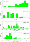 |
Fig. 1. Distribution of the key properties of the QSOFEED sample. From top to bottom, the panels show the distribution in redshift of the sample, in stellar masses of the host galaxies taken from Pierce et al. (2023), in bolometric luminosities, and in 1.4 GHz radio luminosities. Only objects that have either FIRST or NVSS detections are included in the bottom panel and upper limits are given in Table A.1. The mean value for each property is given in the individual panels. |
The black hole masses and Eddington ratios reported in Table A.1 come from Kong & Ho (2018) and were estimated using stellar velocity dispersions measured from SDSS spectra and the MBH-σ* relation. The black hole masses range from 106.8 to 108.8 M⊙ and the Eddington ratios (fEdd) between 0.01 and 4.57. Thus, our QSO2s are near-Eddington to Eddington-limit obscured AGN in the local universe, unlike Seyfert 2 galaxies, which have typical Eddington ratios of fEdd ∼ 0.001 − 0.1. We refer the reader to Ramos Almeida et al. (2022) for more details on the QSOFEED sample.
To carry out this investigation into the stellar populations and gas kinematics in the QSOFEED sample, we downloaded spectra for each object from the SDSS archive. The majority of the spectra (43) are derived from the Legacy survey (Abazajian et al. 2009), which used a 3 arcsec diameter fibre and covered an observed wavelength range of 3800–9200 Å (∼3455 − 8360 Å at the average redshift of the sample, z = 0.11) with a spectral resolution of R = 1800–2200. The remainder of the objects (5) have been observed as part of the Baryon Oscillation Spectroscopic Survey (BOSS; Dawson et al. 2013), which used a 2 arcsec diameter fibre and covered an observed wavelength range of 3600–10 000 Å (∼3270 − 9090 Å at z = 0.11) with a resolution of R = 1300–2600. Where available, the BOSS spectra were used because the extended blue-ward coverage is useful when attempting to detect the presence of young stellar populations (YSPs) and these objects are marked with an asterisk in Table A.1. The wide wavelength coverage means that key features for the modelling of stellar populations are covered, however, the signal-to-noise ratios (S/Ns) of the data vary widely across the sample, ranging from ∼12 − 40. This can have a significant impact on our ability to constrain the proportion of flux allocated to the YSP in the model and, consequently, the star formation rate.
2.2. Stellar populations modelling
Using the same stellar population modelling technique as in Bessiere & Ramos Almeida (2022), we made use of the STARLIGHT (Cid Fernandes et al. 2005) code in conjunction with the Binary Population and Spectral Synthesis (BPASS) synthetic stellar models (Eldridge et al. 2017; Stanway & Eldridge 2018). Before carrying out the modelling, the spectra were first corrected for Galactic extinction using the E(B-V) values of Schlafly & Finkbeiner (2011) and the Cardelli et al. (1989) extinction law and then shifted to the rest frame using the SDSS redshift values. The spectra were then resampled to 1 Å pix−1 as suggested in the STARLIGHT user manual.
We selected BPASS models with a broken power-law inital mass function (IMF) with α1 = −1.30 and α2 = −2.35 and an upper mass cut-off of 100 M⊙, where each template represents a simple stellar population formed in an instantaneous burst of 106 M⊙. Three metallicities were included in the modelling, allowing for sub-solar, solar and super-solar stellar populations (Z = 0.002, 0.02, 0.04) and 27 ages for each metallicity ranging from 1 Myr to 12.5 Gyr, sampled to reflect the rapidity of the evolution of the stellar spectra at young ages. The base templates can then be combined in different proportions by the STARLIGHT code to produce the final model, assuming that: (1) all the templates will be subject to the same reddening or (2) selected templates can have additional reddening applied. Throughout this study, the extinction curve of Calzetti et al. (2000) has been assumed.
To better fit the stellar populations, the nebular continuum and higher-order Balmer emission lines were first modelled and subtracted from the SDSS spectra using the same technique outlined in Bessiere et al. (2017). The most prominent emission lines were masked in this first step. To briefly summarise, initially, there were 50 independent fits to each spectrum carried out, allowing for all ages and metallicities outlined above. In this initial run, it was assumed that templates with ages of < 7 Myr could have additional reddening applied compared to those of older ages. The fit with the lowest χ2/N was then selected as the best fit and subtracted from the data, leaving a pure emission line spectrum. The [OIII]λλ5007, 4959 and Hβ lines were then fit simultaneously, using up to five Gaussian components, applying the standard technique of tying the velocities and widths of the Hβ Gaussian components to those of the [OIII] components. In this way, it is possible to better constrain the fit to the Hβ line when multiple Gaussian components are required to produce an acceptable fit. Assuming Case B recombination (Osterbrock & Ferland 2006), the total flux of the Hβ line (the sum of Gaussian components) is then used to construct the nebular model, which consists of the nebular continuum and the higher-order Balmer emission lines (e.g. H9 (3835 Å), H10 (3798 Å), H11 (3771 Å), and H12 (3750 Å)). The resulting nebular model is then subtracted from the SDSS spectrum, producing the nebular subtracted spectrum used for the remainder of the stellar modelling process. A detailed discussion of the impact of the nebular subtraction on the results of the stellar population modelling is presented in Sect. 3.1.
The next step in the modelling process is determining the best combination of metallicities to fit the nebular subtracted data. To facilitate this, three age bins for the stellar populations were defined, and stellar population templates from each bin were included in all the following modelling step. The defined age bins are: young stellar population (YSP; tysp < 100 Myr), intermediate stellar population (ISP; 100 Myr < tisp < 2 Gyr), and old stellar populations (OSP; tosp > 2Gyr).
A grid of 26 combinations of age bins and metallicities was defined by assigning one of the above metallicities to each age bin in turn. For each combination two scenarios were considered, one in which all the templates were subject to the same reddening and one in which models with ages of < 7 Myr were allowed to have additional reddening, resulting in a total of 54 combinations tested for each spectrum. Each combination was run through STARLIGHT 20 times and the combination that produced the lowest mean χ2/N was selected as the correct stellar model. To estimate the errors on the flux allocated to each of the stellar age bins outlined above, random Gaussian noise (consistent with the SDSS error spectrum) was added to each spectrum 100 times and run again using the same combination of metallicities as found in the previous step. The errors in the proportion of the flux in each age bin are then considered to be the standard deviation of the results of these 100 runs.
Examples of the STARLIGHT fits to the nebular subtracted data are shown in Figure 2, where the left panel shows the fit to J0818+36 in which 7 per cent of the flux in the normalising bin is associated with the YSP, whilst the right panel shows the fit for J1548−01, which has a large contribution from the YSP (88 per cent). In both cases, the bottom panel shows the residuals of the fit, with the grey-shaded areas showing the regions masked out during the fit. The pink-shaded areas show regions given double weighting because they are strongly associated with stellar absorption features not otherwise infilled by emission lines. The green crosses mark pixels flagged in the original SDSS spectrum and masked out of the fit.
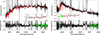 |
Fig. 2. Two examples of the results of the STARLIGHT fitting. The left panel shows the fit to J0818+36, which has a low fraction of YSP (7 per cent), where the top panel shows the data in black and the overall fit in red. The bottom panel shows the residuals of the fit with the residuals in black, the regions masked out during the fit shaded in grey and those that were double-weighted shaded in pink. Pixels flagged in the SDSS spectrum are marked by green crosses and the magenta line marks zero. The inset in the top panel shows the fit in the region of the higher-order Balmer absorption features associated with young stars. The right panel shows the same but for J1548−01, which has one of the highest fractions of YSP (88 per cent). All the STARLIGHT fits are shown in Appendix https://zenodo.org/records/11965868. |
The results of the STARLIGHT modelling also allow us to calculate star formation rates (SFR) within the physical area covered by the SDSS fibre (between 2 and 7 kpc diameters depending on the redshift). We sum the total mass associated with each input stellar template with ages < 100 Myr and divide by 108 years, thereby averaging the SFR over the timescale of interest in this work.
Although all the objects in the QSOFEED sample are obscured, making it unnecessary to introduce a direct AGN component into the stellar modelling, it is not possible to rule out potential contamination of the stellar spectrum by direct AGN light being scattered into our line of sight by the intervening obscuring material. As this scattering is wavelength dependent (Fλ ∝ λα), it would be expected to contaminate shorter (bluer) wavelengths more strongly, thus having the potential to skew the results of the stellar population modelling to younger ages.
Bessiere et al. (2017) carried out a similar study to that presented here based on a sample of 20 QSO2s at slightly higher redshift (0.3 ≤ z ≤ 0.41) within the same AGN luminosity range as those of the QSOFEED sample. In that work, the potential impact of introducing a power-law (PL) component into the model to account for this scattered component was tested by carrying out the population modelling using the same stellar templates both with and without a PL. In common with the QSOFEED sample, it was not possible to impose constraints on either the proportion of the flux contributed by the PL or α as no spectropolarimetric information was available. Therefore, the PL flux was allowed to vary between 0 ≤ PL% ≤ 100 and α between −15 ≤ α ≤ 15. The results of that work clearly demonstrated that the inclusion of an unconstrained PL component results in the modelling becoming highly degenerate between YSP age, YSP reddening, PL flux, and α and thus no meaningful constraints could be placed on the YSP from the modelling alone. For this reason, we do not attempt to include a power-law component into the stellar population modelling.
Although we are unable to place any constraints on a potential scattered AGN component, we are able to make a basic assessment of whether not including a power-law component is a valid assumption. As described above, one of the key steps in performing the stellar population modelling is to produce an emission line spectrum by subtracting the stellar model from the data. Scattered light from the obscured AGN will carry with it the imprint of the broad line region (BLR) and, therefore, we should expect to see some evidence of broad Hβ in the emission line spectrum if a scattered component is contributing strongly to the total observed flux. However, in the individual objects, we do not find evidence of any broad Hβ component in the emission line spectrum and Hβ is well fit using the same kinematic components as those used to fit the [OIII]λλ4959, 5007 emission lines.
However, we would expect traces of a broad Hβ component to be faint, but to become more significant with increasing AGN luminosity. Therefore, as a further check on the potential significance of a scattered component to the total light spectrum, we construct stacks of the Hβ and [OIII] emission lines, consisting of all objects with observed log L[OIII] > 8.9 (8 objects) excluding J1517+33, which has a double peaked [OIII] line profile. These comprise the most luminous objects in the sample, where any contamination in the form of broad Hβ, associated with the BLR, would be most evident.
The stacks for each emission line were generated independently by first normalising the individual spectra to the peak flux of the Hβ or [OIII]λ5007 line and then taking the mean value of flux at each of the pixels (excluding flagged pixels). We then fit an increasing number of Gaussian components to the [OIII] composite, applying the same constraints as outlined in Sect. 2.3, until a reasonable fit was achieved. The resulting model was then applied to fit the Hβ composite, constraining the widths and velocities of each of the Gaussian components to be the same as those obtained from the [OIII] fit, with only the amplitudes of each of the components left as free parameters. The results of this procedure are shown in Figure 3, where the top panel shows the [OIII] composite in black, the total fit in red and the individual components are also shown in different colours. The bottom panel shows the resulting fit to Hβ and the individual components which are constrained to have the same width and velocity as those shown above. The residual of the fits are shown at the bottom of each panel and clearly demonstrate that, even when considering only the most luminous objects in the QSOFEED sample, the Hβ line is well fit using the same components as [OIII] and there is no evidence that a broader component associated with light scattered from the BLR is required to adequately fit the Hβ line.
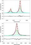 |
Fig. 3. [OIII] (top) and Hβ (bottom) emission line stacks (black) and total fits (red). The individual Gaussian components which comprise the total fit are shown in different colours, with the same components shown in the same colours in both fits. The individual components of the Hβ fit are constrained to have the same width and velocity as those obtained from the [OIII] fit, thereby demonstrating that no additional broad component is required to account for light scattered from the BLR. The residuals are shown underneath each fit. |
As a further check on our assumption that scattered AGN light does not significantly contaminate our results, we test the relationship between L[OIII] and the monochromatic continuum luminosity in the bluest common wavelength bin among the QSO2s (3684–3704 Å). If a scattered component significantly contributes to the total measured light, increasing L[OIII] should be accompanied by increasing near-UV continuum flux because both are powered by the AGN. Therefore, we calculate the Pearson correlation coefficient between the monochromatic luminosity (calculated as the average over the bin) of the continuum and L[OIII] and find r = 0.437, suggesting that no correlation exists between the two. Taking into account the results of the tests presented above, we do not consider the role that scattered light may play in the results of our stellar population analysis further.
The main results of the stellar population modelling are given in Table A.2, which shows whether the Balmer absorption lines were detectable in the unsubtracted data, the proportion of the flux allocated to each age bin, and the SFR calculated from the STARLIGHT results. ΔVSL measures the velocity shift between the data and stellar templates and σSL is the velocity dispersion of the stellar populations. The reddening (AV) and additional reddening (YAV) applied to populations with ages less than 7 Myr, as well as the metallicities of the templates used in each age bin, are also listed.
2.3. Emission line fitting
To measure the kinematics of the warm ionised gas, we adopt a non-parametric approach (Harrison et al. 2014; Zakamska & Greene 2014) to measuring the properties of the [OIII]λ5007 emission line. Initially we define the values V05,V10,V90, and V95, which measure the velocities at the 5, 10, 90, and 95 percentage points of the normalised cumulative function of the emission line flux. V05 and V95 are considered to be the maximum outflow velocities, W80 is a measure of the width of the line containing 80% of the total flux and is equivalent to 1.088 × FWHM = 2.563 × σ (W80 = V90 − V10), whilst ΔV measures the velocity offset of the broad wings of the emission line from systemic (ΔV = (V05 + V95)/2); see Zakamska & Greene 2014 for a detailed explanation). We also measure the asymmetry of the line, which is a measure of the difference of the flux in the blue and red wings of the line as A = |V90 − V50|−|V10 − V50|.
We find a wide range of [OIII] emission line profiles in the QSOFEED sample, which, in some cases, require several Gaussian components to match the profile adequately. Therefore, we first used the IDL non-linear least-squares fitting routine MPFIT (Markwardt 2009) to simultaneously fit the [OIII]λλ4959, 5007 lines, adopting the standard technique of fixing the lines to share the same kinematic components and fixing the flux ratio to a value of 3. We note that we ascribe no physical meaning to the individual components, and are solely concerned with the goodness of the overall fit (as in Harrison et al. 2014). After subtracting the continuum, we begin by fitting two Gaussian components to each line, adding components (up to a maximum of six in total) until the improvement in reduced χ2 < 10%. Each time an additional component was included, the initial input values were randomly generated (within reasonable constraints) and the fit was run nol × 30 times, where nol is the number of Gaussian components. The fit with the lowest reduced χ2 from the nol × 30 runs was the retained model for that number of Gaussian components, and the associated reduced χ2 was used to determine whether the additional component was required.
The resulting [OIII]λ5007 line model, comprising the sum of all Gaussian components, was then used as the basis for the non-parametric measurements outlined above. Figure 4 shows examples of how the method described was carried out, showing two of the diverse objects in the sample. The left column shows the results of the line fitting using MPFIT where the data is shown in black and the total fit is shown in red. The colours of the individual Gaussian components are the same for each line. The right panels show examples of how the non-parametric values were derived, with the model now in black and the grey shaded area representing W80.
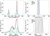 |
Fig. 4. Examples of the emission line fitting technique used. The left panels show examples of the Gaussian fits obtained using MPFIT to J1300+54 and J1347+12, which have the narrowest and broadest line profiles in the sample. The black line shows the data and the red line shows the sum of the Gaussian components which are denoted in shades of blue and green. The red crosses show pixels that were masked out of the fit. The right panels show the corresponding non-parametric values derived from the emission line models. All the emission line fits are shown in Appendix https://zenodo.org/records/11965868. |
In order to estimate the 1σ errors on these non-parametric values, noise was added to the spectrum that was consistent with the SDSS error spectrum and the fit was performed again and the non-parametric values recalculated. This process was repeated 100 times for each of the objects.
2.4. Outflow rates
Using the results of the non-parametric fitting outlined in Sect. 2.3 and the results presented in Table A.3, it is also possible to estimate outflow masses, mass rates, and kinetic energies in the warm ionised gas phase. To make these estimations, it was assumed that all gas at absolute velocities greater than V05 and V95 is outflowing.
To estimate the mass outflow rate, the electron densities were derived separately for each object using the transauroral line technique (Holt et al. 2011; Santoro et al. 2018; Davies et al. 2020; Holden et al. 2023; Holden & Tadhunter 2023), where possible, which is based on the ratio of the fluxes of the transauroral lines (TR([OII]) = [OIII](3726 + 3729)/[OIII](7319 + 7331); TR([SII]) = [SII](4068 + 4076)/[SII](6717 + 6731)). In six cases, it was not possible to use this technique because the required lines were not well detected in the SDSS data, so the [SII](6717/6731) doublet flux ratio was used instead.
Fluxes were measured from the pure emission line spectrum (i.e. data – stellar model) after fitting a first-order polynomial to remove any remaining continuum. In most cases, a single Gaussian profile was fit to each line, however, some cases required an additional Gaussian to account for the entire line profile. This was most often the case when measuring the fluxes of the [SII]6717,6731 doublet, which sometimes required an additional broader component. In cases where it was possible to measure the fluxes of the transauroral lines, the measured fluxes were used to calculate the line ratios which were then compared to those expected from photoionisation models, as first described by Holt et al. (2011). The photoionisation models were created with the CLOUDY code (Ferland et al. 2017), and assume a solar-metallicity, radiation-bounded, single-slab, plane-parallel cloud. The central ionising continuum is assumed to have a spectral index of α = 1.5, and the ionisation parameter is log U = −2.32. The density of the cloud was varied between 2 < log(ne[cm−3]) < 5 and the TR ratios were reddened from the model using the Cardelli et al. (1989) extinction law. The resulting ratios from the model were plotted and the measured ratios from the SDSS spectra were overplotted, with the electron densities being derived from this grid (see Figure 5 in Speranza et al. 2022 for an example).
In a further two cases (J1218+47 and J1316+44), it was not possible to measure the electron density using either technique because the SDSS flags cover the transauroral lines and [SII]6717,6731 doublet, therefore we adopted the mean of the measured values of electron density (ne = 4607 cm−3). The values of electron density derived from the SDSS spectra are shown in Table A.3 where electron densities measured using the [SII](6717/6731) doublet ratio are given between parenthesis. Where we have used the transauroral technique to measure ne, we find values in the range 210 < ne < 38020 cm−3 with a mean value of 4230 cm−3 and using the [SII] ratio we find a range 275 < ne < 550 cm−3, with a mean value of 455 cm−3. Where we have been able to measure ne via both methods, we have found that, on average, the electron density derived using the transauroral technique is 7 times larger than when using the [SII] ratio.
Because we are primarily interested in the high velocity outflowing gas associated with the wings of the line, it would be preferable to measure the emission line ratios used to calculate electron density (for both techniques adopted here) from the wings of the relevant emission lines. However, in practise, this is not feasible as the emission lines can be weak and difficult to deblend. Therefore, the electron densities used in these outflow calculations are derived from the ratios of the total line flux as previously described. However, it should be noted that outflowing gas is denser than non-outflowing gas (Villar-Martín et al. 1999; Speranza et al. 2022; Holden et al. 2023), meaning that we are likely to be somewhat underestimating electron densities.
After correcting the [OIII] emission line model for internal reddening using the E(B-V) values calculated from the Balmer decrements measured when constructing the nebular emission model, we then calculate the total mass of the outflow by integrating the total flux in the blue and red wings of the [OIII]λ5007 emission line model below (above) V05 (v95). After converting this value to a luminosity using the values for luminosity distance given in Table A.1, we use Eq. (1) to calculate the outflow mass (Fiore et al. 2017).
![Mathematical equation: $$ \begin{aligned} M_{\rm [OIII]} = 4 \times 10^7\,M_{\odot } \left(\frac{C}{10^\mathrm{O/H}}\right) \left(\frac{L_{\rm [OIII]}}{10^{44}}\right) \left(\frac{10^{3}}{\langle n_e \rangle }\right). \end{aligned} $$](/articles/aa/full_html/2024/09/aa48795-23/aa48795-23-eq2.gif) (1)
(1)
To then estimate the total ionised gas mass of the outflows, we assume that it is three times the [OIII] outflow mass (Mof = 3 × M[OIII]; Fiore et al. 2017). The velocity of the outflowing gas (v50) is estimated as the 50 percentile of the cumulative function of the flux between the continuum and V05 or V95 in the blue and red wings of the line independently, following Hervella Seoane et al. (2023) and Speranza et al. (2024). The kinetic energy of the outflow is then,
 (2)
(2)
The estimate of mass outflow rates and the kinetic energy they carry is dependent on the physical size of the outflow (Eqs. (3) and (4)). The use of SDSS spectroscopy in this study precludes the ability to measure the sizes of the outflow regions. However, using a combination of HST narrow-band imaging and STIS long-slit spectroscopy, Fischer et al. (2018) measured the sizes of the outflow regions in a sample of 12 QSO2s that also form part of the QSOFEED sample. They found deprojected outflow sizes ranging from 0.15–1.89 kpc, with a mean and median of 0.62 and 0.57 kpc respectively, although in 10/12 cases, the outflow radii are less than 1 kpc. Therefore, when estimating the mass outflow rates in the QSOFEED sample, here we assume an outflow radius of 0.62 kpc, so the mass outflow rate and kinetic power are given by,
 (3)
(3)
 (4)
(4)
The values for the blue and red wings of the lines are calculated independently and then summed to obtain the total values which are given in Table A.3. Figure 5 demonstrates how this process was carried out, where the flux in the regions shaded in blue and red were integrated to determine the luminosities as input for Eq. (1). The solid blue and red lines mark the v50, blue and v50, red velocity values that are used as the outflow velocities in Eqs. (2)–(4).
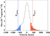 |
Fig. 5. Example of how outflow fluxes and velocities were calculated. The black line shows the model of the [OIII]λ5007 emission line and the blue and red shaded regions show the velocities at which gas is considered to be included in the outflow. The solid blue and red lines represent v50, blue and v50, red which are the outflow velocities. |
3. Results
The aim of this work is to not only characterise the stellar populations and warm ionised gas kinematics of the full QSOFEED sample, but to also compare the results of these two strands of investigation to clarify whether evidence that the presence of the AGN is directly impacting star formation can be established. Due to the likely timescales associated with AGN feedback, we are primarily concerned with the YSP because this is the population that will potentially be affected by the presence of AGN-driven outflows.
3.1. Stellar populations
The results of the stellar population modelling are given in Table A.2, which shows the percentage of the total flux allocated to each age bin (before reddening), at the normalising wavelength, as well as the extinction (AV) and additional extinction (YAV) applied by STARLIGHT to the populations with ages < 7 Myr (where applicable). In total, we find that 47/48 (98 per cent) of the objects in the QSOFEED sample require the inclusion of a YSP younger than 100 Myr in order to adequately model their SDSS spectrum. If we further discount J0052−01, which has a YSP flux consistent with 0 per cent within the errors, we find that 46/48 (96%) of the objects then require the inclusion of a YSP. Figure 6 shows the proportion of the total flux associated with the YSP, which varies between 0 and 100 per cent, against the current stellar mass within the SDSS aperture, whilst the right panel shows the SFR within the SDSS aperture, which ranges between 0 and 92 M⊙ yr−1, against the stellar mass contained within the aperture.
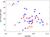 |
Fig. 6. Proportion of the flux that is attributed to the YSP by the STARLIGHT modelling against the current stellar mass within the SDSS aperture. Red symbols represent undisturbed host galaxies whilst blue represent merging systems. J1034+60 (Mrk 34) is represented by a cyan star (see Sect. 4.2) for details. |
A full morphological classification of the QSOFEED sample, based on deep optical imaging, has been presented in Pierce et al. (2023) and in order to understand whether a host galaxies’ interaction status is a determining factor in the stellar and/or gas kinematic properties found in this work, we have differentiated between these groups. Throughout this work, unless otherwise stated, blue symbols denote QSO2 host galaxies that have been classified as morphologically disrupted (i.e. evidence of galaxy mergers), whilst red symbols denote the galaxies that have been classified as morphologically undisturbed.
SFRs for seven of the objects were also measured in Ramos Almeida et al. (2022) using rest frame infrared (IR) luminosities and in one case (J0232−08), we find a significantly higher SFR (33 M⊙ yr−1) than that measured from the IR (3 M⊙ yr−1). A potential reason for this difference is that this object may be a case where a scattered AGN component is a significant factor and we have not accounted for it in our modelling. In the remainder of the cases, our results are either consistent with or less than the SFR that was found in Ramos Almeida et al. (2022). When considering this, we must bear in mind that, when calculating the SFR from IR luminosities, the flux of the entire galaxy is taken into account, whereas the SFRs calculated from the SDSS spectra only include the SF encompased by the fibre. It could be that in these cases, the SF is distributed throughout the galaxy rather than in the central region on which the fibre is trained.
The objects in the QSOFEED sample were not selected based on any property of their host galaxies, only on AGN luminosity and redshift. This results in a sample which includes a range of host galaxy morphologies, as well as mergers and non-mergers. These are properties that play an important role in star formation. Both simulations and observations show that, under certain conditions, galaxy mergers can trigger rapid star formation. As at least 65% of the QSOFEED sample show morphological disruption consistent with merger activity, it is instructive to consider whether mergers have a more significant impact on the SFR of a QSO2s host galaxy than any properties associated with the AGN. To test this, after excluding the three objects in which the SFR is unconstrained, we split the sample into undisturbed (15) and merging (30) galaxies and find a mean SFR of 18.5 ± 12.4 = M⊙ yr−1 (median of 16.5 M⊙ yr−1) for the undisturbed QSO2s and of 2..5 ± 21.0 = M⊙ yr−1 (median of 20.8 M⊙ yr−1) for the disturbed QSO2s. A two-sided K-S test returns D = 0.200 with a significance P = 0.771, so we do not find a significant difference between the SFRs of merging and non-merging galaxies in this sample.
The QSOFEED galaxies vary in physical size, while the range of redshifts and the use of spectra from both the Legacy (3 arcsec fibre) and BOSS (2 arcsec fibre) archives means that the physical scale covered by the SDSS fibre varies from object to object. The SDSS r-band Petrosian radius (Petrosian 1976) measures the radius at which the local surface brightness is equal to 0.2 times the mean surface brightness within that radius, so if we consider this to be a reasonable measure of the size of the galaxy, the physical diameters of the hosts are in the range 6.3–56 kpc with a mean of 18 kpc, whilst the physical scales covered by the SDSS fibres are 2.2–7.4 kpc with a mean of 5.6 kpc. If we make the assumption that all the star formation occurring within the galaxy is captured by the SDSS fibre (although this may be a lower limit), we can compare the values obtained to the main sequence of galaxy formation to gain an insight into whether the outflows driven by the QSO2s affect SF in their host galaxies. If this lower limit puts the galaxies on or above the expected main sequence values, then this is an indication that SF is not being suppressed. However, for galaxies that lay below the relation, we cannot definitively conclude that SF is being suppressed as it may instead be the case that all the SF that is occurring has not been captured. Figure 7 shows the SFR against the total mass of the host galaxies (Pierce et al. 2023), where the colour scale shows the ratio of the physical scale covered by the fibre and the Petrosian radius. The main sequence defined in Saintonge et al. (2016) is shown as the solid black line with the dashed black lines showing the range of main sequence values (±0.4 dex). As can be seen, the majority of the objects in the sample (47/48) lie on or above the main sequence except for one object in which no star formation activity is detected within the previous 100 Myr. These findings suggest that the QSOFEED host galaxies are still actively forming stars and in some cases, at rates usually associated with luminous or ultra-luminous galaxies (U)LIRGs (Ramos Almeida et al. 2022; Lamperti et al. 2022).
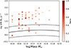 |
Fig. 7. SFR measured from the STARLIGHT modelling of the SDSS spectra against the total stellar mass of the host galaxies (Pierce et al. 2023). The colour scale shows the ratio of the physical size on the galaxy covered by the SDSS fibre against the r-band Petrosian diameter. The black solid line shows the SF main sequence (MS) defined in Saintonge et al. (2016) and the dashed black lines the range of SFR that is considered to cover the MS (±0.4 dex). |
In addition to considering the absolute proportion of flux allocated to the YSP by the STARLIGHT modelling, Table A.2 shows whether it is possible to detect the presence of the higher-order Balmer absorption features in the spectrum before nebular subtraction for each object. This feature is indicative of the presence of YSPs and therefore, it is instructive to consider what proportion of the objects have detectable Balmer absorption lines as an independent check. We find that 26/48 (54 per cent) of the sample clearly show the presence of Balmer absorption lines in their spectra before nebular subtraction, which increases to 42/48 (88 per cent) after the nebular subtraction, consistent with the proportion determined by the spectral synthesis modelling.
To understand why this significant increase in detection occurs after nebular subtraction, the left panel of Figure 8 shows an example of the nebular subtraction process for an object in which the Balmer absorption lines were not detected in the original data but became apparent when the nebular subtraction process was carried out. The black line shows the original data, the blue line is the model of the nebular continuum and higher-order Balmer emission lines, and the red line shows the nebular subtracted data. This example illustrates the impact of the removal of the emission line infilling of the underlying stellar absorption features and also the reduction in the total continuum flux below the Balmer edge (3646 Å). These two effects have differing results on the final model because the increase in the strength of the stellar Balmer absorption features (if this occurs) will result in the final stellar population model being more weighted towards younger stellar ages, whilst the reduction in the near-UV flux has the opposing effect. The right panel of Figure 8 shows the impact that the nebular subtraction procedure has on the proportion of the flux in the normalising bin that is allocated to the YSP by STARLIGHT both before and after the nebular subtraction. The black line shows the one-to-one relation and demonstrates the importance of considering nebular contamination of the stellar component when attempting to characterise the stellar populations of QSO2s host galaxies. Failure to do so can result in significant over or under-estimations in flux associated with the YSP.
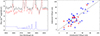 |
Fig. 8. Example of the impact of the nebular subtraction process on the SDSS spectrum of J1316+44 (left). The black and red lines show the original and nebular subtracted data, while the blue line shows the subtracted nebular model. A comparison of the percentage of the total flux allocated to the YSP in the unsubtracted and nebular subtracted data is shown on the right. The black line shows the one-to-one relation between the two values. Red and blue points represent objects classified as morphologically undisturbed and disturbed, respectively. |
3.2. Gas kinematics
As previously stated, we find a wide variety of [OIII] line profiles in the QSOFEED sample and therefore, a wide range of gas kinematic properties. Table A.3 shows the results of the non-parametric analysis of these line profiles. There is a wide variety in the widths of the [OIII] emission lines, ranging from 300 < W80 < 2500 km s−1, with a mean value of 804 km s−1 (median 717 km s−1).
Figure 9 shows a comparison of W80 and the velocity dispersion of the stellar component of the host galaxy (W80SL = 2.563σSL) as measured from the STARLIGHT modelling of the SDSS spectra. The black line shows the one-to-one relation between the two properties and demonstrates that, in the majority of cases, the [OIII] dispersion is higher than would be expected purely from the dispersion of the galaxy. We find that in 41/48 (85%) of cases, the dispersion of the [OIII] line lays above the one-to-one relation, suggesting that the ionised gas in these galaxies is outflowing, driven either by the AGN, star formation, or a combination of both. For comparison, if we require W80 > 600 km s−1 for the gas to be considered outflowing (as in Harrison et al. 2016; Kakkad et al. 2020; Scholtz et al. 2020) the percentage of QSO2s with ionised outflows would be 67% (see Table A.3).
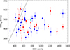 |
Fig. 9. Results of the non-parametric [OIII] line measurements compared to the velocity dispersion of the stellar component of the host galaxies measured by STARLIGHT. The black line shows the one-to-one relation between the two values. Note that for presentation purposes, J1347+12 has been omitted from this plot due to it’s high value of W80 (≈2520 km s−1). |
When we consider the W80 values, where W80 is larger than W80SL, in the merger and non-merger groups separately, we find that in the merging galaxies (27), the mean W80 is ≈837 km s−1 (median 763 km s−1) whilst in QSO2s classified as undisturbed (14), the mean W80 is ≈909 km s−1 (median 853 km s−1). A Kolmogorov–Smirnov (K-S) test to determine whether the W80 values for the disturbed and undisturbed groups of galaxies are drawn from the same underlying distribution returns p = 0.57, so we conclude that there is no significant difference between W80 in merging and non-merging galaxies, suggesting that mergers are not the dominant cause of the disrupted gas kinematics observed.
The QSOFEED host galaxies cover the range of stellar masses 10.6 < log(M/M⊙) < 11.7 and more massive galaxies will have a higher intrinsic stellar velocity dispersion, therefore higher values of W80 do not necessarily indicate broader widths in relation to those that should be expected from that of the underlying host galaxy. To investigate this, we define the term  , thereby deconvolving the galaxy and [OIII] velocity dispersions. When considering the 41 galaxies where W80 > W80SL, we find the values of W80int in the range 260–2460 km s−1 with a mean 714 km s−1 and a median of 613 km s−1, demonstrating that, in the majority of the QSOFEED sample, the velocity dispersion of the gas is significantly higher than that of the stellar component of the host galaxy, suggesting the presence of powerful AGN-driven outflows.
The SDSS pipeline uses various stellar and emission line features to compute redshifts, which works well when the emission lines are narrow and symmetric. However, in cases where emission lines are asymmetric, this can lead to errors in the derivation of the redshifts. When carrying out the stellar population modelling, the emission lines are masked and the code relies solely on the stellar absorption features to determine how much to shift the synthetic templates to match the data, making the STARLIGHT velocity shifts (ΔVSL; Table A.2) a more accurate estimate of the systemic velocity of the host galaxy. Therefore, we define the property ΔVdiff = ΔV[OIII] − ΔVSL which is a measure of the velocity shift of the wings of the emission lines ΔV[OIII] relative to ΔVSL as a measure of whether the velocity of the ionised gas is shifted relative to the host galaxy, which we consider to be indicative of outflowing gas. Four of the objects (J0805+28, J1015+00, J1100+08, and J2154+11) have [OIII] emission line velocity shifts consistent, within the errors, with that of the underlying host galaxy (ΔVdiff ∼ 0) and the shift is likely to be smaller when ΔVSL is close to 0, as expected for the reasons outlined above (see left panel of Figure 10). However, it is interesting to note that these four objects all have values of W80 than are higher than those expected purely from the dispersion of the host galaxy (see right panel of Figure 10). In particular, J1100+08 has ΔVdiff = 16 ± 18 km s−1 whilst the W80 = 1082 ± 7 km s−1 which is significantly higher than the W80SL = 422 km s−1 found from the STARLIGHT modelling. It is possible that the reason that the [OIII] emission line is so broad whilst still being at the systemic velocity of the galaxy because the outflow that it is tracing is spherically symmetric.
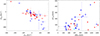 |
Fig. 10. Difference in the velocity offset of the [OIII] emission line and that of the host galaxy (left). The right panel shows the deconvolved W80int values against |ΔVdiff|, where |
Taking the above into account, we therefore only consider the condition that W80 > W80SL as determining whether it is considered that an outflow has been detected, meaning that 85% of the QSO2s host outflows. However, the nature of the SDSS data means that we are unable to place constraints on the sizes of these outflows.
3.3. Correlations
The key question the QSOFEED project aims to investigate is how do luminous AGN impact their host galaxies?, requiring us to consider two distinct aspects. Firstly, we must investigate whether QSO2s can drive significant outflows and, secondly, whether those outflows directly impact star formation. Therefore, in this section, we consider whether there are any correlations between the kinematics of the warm ionised gas and the intrinsic properties of the QSO2s (e.g. bolometric luminosity and Eddington ratio). We then compare SFRs with the kinematics of the warm ionised gas to investigate whether any correlations exist between these two properties.
3.3.1. AGN properties and gas kinematics
To determine whether the gas kinematics are dependent on the AGN properties, we calculate the Pearson correlation coefficients (r) between intrinsic AGN characteristics (Lbol, L1.4 GHz, MBH, λ/λEdd) and the ionised gas kinematics derived in this study (W80int, ΔVdiff, Ėkin, and Ṁof) for the 41 QSO2s in which outflows were detected. The resulting correlation coefficients for each combination of parameters tested are given in Table 1.
Pearson correlation coefficients between the various outflow properties and intrinsic properties of the AGN.
The results presented in Table 1 demonstrate that no strong correlations (r > 0.7) exist between the gas kinematics and AGN properties. The strongest correlation found is between L1.4 GHz and W80int, which is shown in Figure 11, where r = 0.58, followed by that between L1.4 GHz and Ėkin, where r = 0.48. This may indicate that radio luminosity is the most significant factor in driving outflows (Mullaney et al. 2013) or alternatively, that the outflows might be inducing shocks in the ISM that produce radio emission (Fischer et al. 2023). The majority of the QSOFEED sample are radio-quiet, however, three objects are classified as radio-loud (J0939+35, J1137+61, and J1347+12), with only J1347+12 exhibiting an outflow. Whilst J1347+12 is a compact steep spectrum source (CSS), the other two are FRII sources, with large-scale radio jets extending beyond the physical scale of the galaxy.
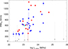 |
Fig. 11. Derived W80int against observed L1.4 GHz, demonstrating the positive correlation between radio luminosity and disrupted gas kinematics. Grey symbols indicate objects in which no outflow was detected according to our criterium. |
Potentially, the radio output of a QSO2/host galaxy can be powered by accretion onto the BH, star formation or a combination of the two, creating a possible source of confusion when attempting to interpret the weak correlation between L1.4 GHz and W80int. To overcome this, we utilise the relation between SFR and L1.4 GHz derived by Davies et al. (2017), using a sample of non-AGN galaxies, to investigate this potential correlation in greater depth. Using the SFRs presented in Table A.2, we calculate the 1.4 GHz radio luminosity expected from star formation alone (L1.4 GHz, SF), allowing us to calculate the 1.4 GHz luminosity attributable solely to the AGN (L1.4 GHz, AGN), so that log L1.4 GHz, AGN = log(L1.4 GHz, obs − L1.4 GHz, SF), where L1.4 GHz is the observed luminosity (see Table A.1). We use these values to calculate r between log L1.4 GHz, AGN and W80int (for objects with outflows) and find r = 0.665. Although still not considered a strong correlation, the fact that it is strengthened when only considering the radio luminosity of the AGN demonstrates that this is likely to be the dominant factor. To further emphasise this point, we consider the correlation between L1.4 GHz, SF and W80int, which yields r = 0.170, demonstrating that it is not the radio luminosity generated by SF that is driving these outflows.
In a recent work, Hervella Seoane et al. (2023) searched for correlations between AGN, host galaxy, and outflow properties in a sample of 19 QSO2s of the same luminosity as the QSOFEED sample and at redshift z = 0.3–0.41. Based on the Spearman’s rank correlation coefficients (ρ), they found moderate correlations between the bolometric luminosity of the AGN and the outflow mass and outflow rate, both with ρ = 0.52. This implies that more luminous AGN have more massive ionised outflows and higher outflow mass rates. On the other hand, Hervella Seoane et al. (2023) did not find any correlation between the radio luminosity and the outflow properties.
3.3.2. Gas kinematics and star formation rates
Having compared the properties of the ionised gas with the properties of the AGN itself, we must now consider whether the detected outflows have an impact on the SFR. If AGN-driven outflows are responsible for quenching star formation, then it may be reasonable to assume that the more powerful the outflow, the more likely it is to directly impact the star formation. In Sect. 3.2, we have measured the kinematics of the ionised gas and derived outflow rates and kinetic energies. Here we compare the results obtained for the outflows with the SFR.
Table 2 shows the Pearson correlation coefficients between SFR, W80int, |Vdiff|, and Ėof, where only objects with detected outflows are considered. These results clearly demonstrate that no correlations are found between the key properties of the ionised gas and SFR in QSO2 host galaxies. These findings strongly suggest that the AGN-driven outflows do not directly impact SF on global scales, even at the highest outflow velocities and energies detected in the QSOFEED sample.
Pearson correlation coefficients between the star formation rate and various properties of the outflows.
However, thus far, we have considered YSPs to be populations with ages < 100 Myr. We must consider the possibility that this timescale is too long in comparison to the predicted lifetime of an AGN and the gas outflow that it drives, which may have the effect of washing out evidence of the direct impact of outflows on SF. Indeed, the measurements of the dynamical timescales of the ionised and cold molecular outflows reported in the literature for QSO2s when outflow radii have been constrained from observations are of ∼1–20 Myr (Bessiere & Ramos Almeida 2022; Ramos Almeida et al. 2022; Speranza et al. 2024). Therefore, we also calculated the SFRs on timescales of 10 and 50 Myr and calculate the Pearson correlation coefficients against the same outflow properties. These values are also given in Table 2 as SFR10 and SFR50 and show that considering timescales that may be more in line with the lifetime of AGN-driven outflows does not lead to any significant change in the level of correlations between SFRs and outflow properties.
4. Discussion
In Sect. 3, we derive the SFR, gas kinematics, and outflow properties of the QSOFEED sample and tested for correlations between these properties. Our objective here is to investigate whether luminous quasars drive outflows and whether, in turn, these outflows directly impact SF. Here, we discuss our findings, making a comparison with the results of previous studies and evaluating them in the context of galaxy evolution.
4.1. AGN and outflow properties
Due to the perceived importance of AGN feedback in galaxy evolution, there have been a wealth of studies aimed at quantifying the properties of AGN-driven outflows, particularly in the warm ionised gas phase (see Harrison et al. 2018 for a review). Although these works adopt different approaches to characterising outflow kinematics, they unanimously conclude that gas outflows are a common phenomena in AGN, and practically ubiquitous at high bolometric luminosities. In common with these works, we also find that outflows in the warm ionised gas phase are a common occurrence in QSO2, with 85% of the sample having [OIII] line profiles that cannot be explained solely by the underlying gravitational potential of the galaxy.
The analysis of [OIII] kinematics presented here has enabled us to calculate mass outflow rates and outflow kinetic powers. However, although we find clear evidence for fast outflows in the majority of the QSOFEED objects, this does not translate to high mass outflow rates or kinetic powers (see Tables 3 and A.3). One key reason for the discrepancy between the outflow rates presented here and those found in various previous studies is the electron densities used to calculate outflow rates. Previous studies have commonly made use of the [SII](6717/6731) ratio to determine electron densities, however, this technique leads to saturation at ne > 103 cm−3, often leading to low (∼200–500 cm−3) densities being estimated or assumed. In this work, where possible, we have measured electron densities using the transauroral technique, which is sensitive to higher electron densities than the [SII] ratio. Densities measured using this technique are, in general, an order of magnitude larger than those assumed by previous studies. Equation (1) in Sect. 2.4 demonstrates the significant impact that this assumption has on the calculated total outflow mass, as the outflow mass decreases with increasing electron density.
Summary of the main results.
Another factor in the discrepancies between the mass outflow rates detected in this study and the significantly higher mass outflow rates detected in other works might be how we determine which gas is considered to be outflowing. Here, we have made conservative estimates of the gas that is included in the outflow by assuming that only gas that has velocities below V05 and above V95 can be considered to be outflowing. For comparison, in Table D.1 of Appendix https://zenodo.org/records/11965868 we report the outflow mass rates and kinetic energy rates calculated by assuming that all gas with velocities greater than 1.5 times the FWHM of the stellar features derived from the STARLIGHT modelling is outflowing. In principle, this approach is less conservative than the one that we considered, but the results are similar. We also checked that the correlation coefficients do not vary by using this outflow definition.
Finally, something that might contribute to explaining the relatively low values of the outflow mass rates and kinetic energies is having characterised the bulk velocity of that gas as the velocity at the 50 per cent cumulative function between the continuum and V05(V95). These assumptions result in lower estimates of the total mass in the outflow, which is calculated from the total luminosity of [OIII] in the wings, and lower outflow velocities than those calculated using parametric methods and maximum velocities (vof = vs + 2σ or vof = vs + FWHM/2) leading to lower mass outflow rates (see Hervella Seoane et al. 2023 for a comparison of the different outflow properties using parametric and non-parametric methods).
A number of works claim positive correlations between outflow kinematics and intrinsic AGN properties, such as the luminosity and Eddington ratio, with more powerful AGN driving more powerful outflows (Cicone et al. 2014; Fiore et al. 2017; Davies et al. 2020; Hervella Seoane et al. 2023). In contrast, when we tested for correlations between these intrinsic parameters in the QSOFEED sample and the various outflow properties here considered, we found no such correlations. Potentially, our contrasting result can be explained by the differences in the AGN luminosity ranges covered by the samples used in these studies. The QSOFEED sample was selected based on redshift and L[OIII], ensuring it contains only the most luminous AGN in the nearby Universe. The consequence of our selection criteria is that L[OIII] covers one order of magnitude (42.1 ≤ log L[OII]I ≤ 42.9 erg s−1), whilst works that claim such correlations tend to cover a broader range of luminosities. For example, the sample analysed by Jin et al. (2023) covers the luminosity range 41.5 ≤ log L[OII]I ≤ 44.0 erg s−1, thus extending to significantly lower luminosities than QSOFEED, and Davies et al. (2020) compiled mass outflow rates for AGN covering 5 orders of magnitude in Lbol. Therefore, we must consider the possibility that the luminosity range probed in this investigation is too small to detect any such correlation.
Although not a selection criterion for QSOFEED, the sample probes a significantly broader range of radio luminosities (22.3 ≤ log L1.4 GHz ≤ 26.2 W Hz−1 for detected sources) than AGN luminosities, giving us increased scope to investigate the dependence of outflow strength on radio power. Previous work has shown that the width of the [OIII] emission lines correlates with radio-luminosity (Mullaney et al. 2013; Zakamska & Greene 2014). Mullaney et al. (2013) used stacked SDSS spectra of thousands of AGN to measure emission line profiles as a function of several variables, including L1.4 GHz, and found that the width of the [OIII] emission line increased as a function of radio-luminosity at intermediate radio luminosities (up to log L1.4 GHz ∼ 25 W Hz−1), declining again at higher radio luminosities. Those findings are consistent with the results presented here, where we see a moderate positive correlation between L1.4 GHz and W80int at intermediate radio luminosities, which strengthens when radio emission associated with star formation is accounted for. Interestingly, the two objects which harbour large-scale radio jets (log L1.4 GHz > 25 W Hz−1) have W80int values which are consistent with those of the stellar velocity dispersion.
We can understand this correlation in the context of simulations which investigate the interaction between low-power radio jets and the host’s ISM (Mukherjee et al. 2016; Talbot et al. 2022). Such simulations indicate that low-power jets will remain confined within the ISM longer than their high-power counterparts, which will rapidly punch through the intervening material. The increased time that the low-power jet remains trapped means it will be more disruptive, impacting a larger volume of the host’s ISM, injecting more turbulence and leading to the broader [OIII] line profiles observed.
However, not all studies comparing the outflow kinematics with radio luminosity find a similar correlation. Ayubinia et al. (2023) compare the [OIII] profile of a large sample of AGN against their radio properties and, in contrast to the results presented here, claim that accounting for the underlying galaxy gravitational potential weakens the positive correlation between the two and instead, it is the Eddington ratio that correlates most strongly with [OIII] velocity dispersion. However, even though we account for the underlying gravitational potential, we still find a moderate correlation between the W80int and L1.4 GHz. This correlation, together with the lack of it between [OIII] kinematics and other properties of the QSOFEED sample, such as Eddington ratio, MBH, and Lbol suggests that small-scale (kpc), low-power radio jets may play an important role in driving outflows. Indeed, this finding is supported by observational studies in both the ionised (Jarvis et al. 2019; Cazzoli et al. 2022; Speranza et al. 2022) and molecular (Morganti et al. 2005; García-Burillo et al. 2019; Audibert et al. 2023) gas phases. However, as mentioned before, it is also possible that not all the kiloparsec-scale radio structures that we see in radio-quiet AGN are jets, but synchrotron radiation produced when the multi-phase outflows interact with the ISM (Zakamska & Greene 2014; Fischer et al. 2023). This would also explain the spatial coincidence between the extended radio structures and the gas outflows and the correlation.
4.2. Star formation and outflow properties
As we have shown, although there is clear evidence that AGN have the potential to drive fast ionised outflows, it is not clear that these outflows directly suppress SF. We have shown that 98 per cent (92 per cent excluding those with unconstrained SFRs) of the galaxies contain stellar populations with ages < 100 Myr, consistent with the results of previous studies of YSPs in QSO2 (Bessiere et al. 2014, 2017; Woo et al. 2020; Jin et al. 2023). Bessiere et al. (2017) used apertures of a fixed physical scale (8 kpc) in their study of the stellar populations of 21 QSO2s at 0.3 < z < 0.41 and found that to adequately fit the data, 71 per cent required the inclusion of a YSP < 100 Myr. The ability to control the physical size of the region probed allowed the authors to make direct comparisons between objects, however, when utilising SDSS spectra to measure stellar populations and gas kinematics, we have no control over the physical scale of the galaxy covered by the fibre. In addition, all spatial information is lost, since the fibre is collapsed to a 1d spectrum. When considering the relationship between AGN-driven outflows and SF, it is most likely that this will be traced within the central few kiloparsecs rather than on galaxy-wide scales as observational evidence from spatially resolved studies demonstrates (Bessiere & Ramos Almeida 2022; Ramos Almeida et al. 2022).
Previously, we have carried out a spatially resolved study of both the ionised gas kinematics and stellar populations of the nearby (z = 0.050) QSO2 Mrk 34 (Bessiere & Ramos Almeida 2022), which forms part of the QSOFEED sample (J1034+60). In that work, we demonstrated a clear spatial correlation between the edges of the approaching side of the kiloparsec-scale ionised outflow (tdyn ∼ 1 Myr) and an enhancement in the fraction of the stellar light attributable to the YSP (ages of ∼1–2 Myr as constrained from the modelling). On the other hand, at the edges of receding side of the outflow, where the turbulence and the energy injection are higher, we do not find the same enhancement of the YSP flux. Here, we have analysed the available SDSS spectrum of Mrk 34 in the same manner as the remainder of the QSOFEED sample as presented above. In Figures 6, 8, 9, 10, and 11, Mrk 34 is plotted as a cyan star and clearly shows that, when using the integrated fibre spectrum to characterise the outflows and YSP, it does not appear to be in any way different from the other objects in the sample. It is only through the use of spatially resolved information that we can detect the positive and/or negative impact that the AGN-driven outflow is having on star formation in the host galaxy. This suggests that it is imperative to increase the number of spatially resolved studies as the one presented in Bessiere & Ramos Almeida (2022), measuring both gas kinematics and stellar populations, to expand our understanding of if, how and under which circumstances AGN-driven feedback directly impacts SF. The advent of the James Webb Space Telescope (JWST) now makes this type of studies possible at high redshift (e.g. D’Eugenio et al. 2023).
Another, yet related to the previous one, possible explanation for the lack of correlation between the outflow properties and SFR is that the effect of AGN on SF is a cumulative rather than an instantaneous process (Scholtz et al. 2020, 2021; Lamperti et al. 2021; Baker et al. 2023). AGN are now thought to be episodic events that can happen throughout the life of a galaxy, flickering on time-scales as short as 105 years (Hickox et al. 2014). Observationally, when investigating the impact of the AGN on the host galaxy, we are only able to probe the effects of the current episode of activity, only allowing for the possibility of characterising direct impacts on the host galaxy (Harrison & Ramos Almeida 2024). However, if the effects are accumulated over several AGN episodes, it may be that SMBH mass is a more relevant indicator because it is through episodes of accretion, leading to AGN activity, that SMBH grows their mass (Martín-Navarro et al. 2021; Piotrowska et al. 2022; Bluck et al. 2022). If the series of AGN episodes has led to the removal and/or heating of the gas, leading to a suppression of SF over time, we would expect to find older populations associated with more massive BHs as the capacity to form new stars is reduced. Indeed, studying the star formation histories of nearby massive galaxies with accurate BH mass measurements, Martín-Navarro et al. (2018) showed that quenching of star formation takes place earlier and more efficiently in galaxies that host higher-mass central black holes. To test this hypothesis in the QSOFEED sample, we calculated the light-weighted ages of each of the QSO2s and found a moderate positive correlation (r = 0.572) with the BH mass, shown in Figure 12. Although many other factors, such as galaxy morphology and merger history also play an important role in the constituent stellar population, this finding could be interpreted as evidence that successive AGN episodes lead to the suppression of SF over the course of galaxy evolution.
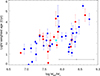 |
Fig. 12. Light-weighted ages of the stellar populations of the QSOFEED sample as a function of black hole mass. A moderate positive correlation, with a Pearson coefficient of r = 0.572 is found. The average error in the black hole mass measurements is shown by the black bar in the lower right corner, with an average error of ±0.48 dex. |
5. Conclusions
In this investigation, we derive the stellar population ages and SFR, warm ionised gas kinematics, and outflow rates for a complete sample of 48 low-redshift, obscured quasars. We compare the results of both strands of the investigation to gain insight into whether AGN-driven outflows directly impact SF in their host galaxies. The key findings of this study can be summarised as follows.
-
Our starlight modelling shows that 98% of the QSOFEED galaxies contain a stellar populations younger than 100 Myr, with percentages of light fraction ranging from 0% to 100%.
-
98% of the QSO2s lay on or above the main sequence of SF.
-
When taking into account stellar velocity dispersion, we find that 85% of the QSO2s show evidence of ionised outflows.
-
In the majority of cases, we use a technique involving the transauroral lines of [OII] and [SII] to determine electron densties and find that these are significantly higher than often assumed, with a mean value of 4230 cm−3.
-
Assuming an outflow radius of 0.62 kpc, we find mass outflow rates for the QSOFEED sample ranging from 0.04 to 1.9 M⊙ yr−1, with a mean of 0.5 M⊙ yr−1.
-
We find no correlation between AGN luminosity, black hole mass or Eddington ratio and the kinematics of the warm ionised gas and/or outflow kinetic powers.
-
We do find a moderate positive correlation between L1.4 GHz and W80int, suggesting that radio luminosity is the most significant factor in driving ionised outflows.
-
We do not find a correlation between the outflow properties and SFR, suggesting that AGN-driven outflows do not directly suppress SF on the physical scales probed by this study.
-
We find a moderate positive correlation between the light-weighted age of the QSO2s’ stellar populations and BH mass, which might be an indication that successive AGN episodes lead to the suppression of SF over the course of galaxy evolution.
Calculated either from the Faint Images of the Radio Sky at Twenty-cm (FIRST; Becker et al. 1995) or NRAO VLA Sky Survey (NVSS; Condon et al. 1998) fluxes of the sample.
While this choice of parameters is an assumption, it only affects the derived densities by 0.1–0.3 orders of magnitude (see Appendix B in Santoro et al. 2020). However, if the gas is ionised by shocks rather than photoionised as we assume, the derived densities will vary by a factor of 2 (Holden & Tadhunter 2023).
Acknowledgments
The authors would like to thank the anonymous referee for their insightful and constructive feedback, enabling them to enhance and refine the results presented here. PSB and CRA acknowledge the projects “Feeding and feedback in active galaxies”, with reference PID2019-106027GB-C42, funded by MICINN-AEI/10.13039/501100011033, “Quantifying the impact of quasar feedback on galaxy evolution”, with reference EUR2020-112266, funded by MICINN-AEI/10.13039/501100011033 and the European Union NextGenerationEU/PRTR, “Quasar feedback and molecular gas reservoirs”, with reference ProID2020010105, ACCISI/FEDER, UE from the Consejería de Economía, Conocimiento y Empleo del Gobierno de Canarias and the European Regional Development Fund (ERDF), and the Agencia Estatal de Investigación of the Ministerio de Ciencia, Innovación y Universidades (MCIU/AEI) under the grant “Tracking active galactic nuclei feedback from parsec to kiloparsec scales”, with reference PID2022-141105NB-I00 and the European Regional Development Fund (ERDF).
References
- Abazajian, K. N., Adelman-McCarthy, J. K., Agüeros, M. A., et al. 2009, ApJS, 182, 543 [Google Scholar]
- Audibert, A., Ramos Almeida, C., García-Burillo, S., et al. 2023, A&A, 671, L12 [NASA ADS] [CrossRef] [EDP Sciences] [Google Scholar]
- Ayubinia, A., Woo, J.-H., Rakshit, S., & Son, D. 2023, ApJ, 954, 27 [NASA ADS] [CrossRef] [Google Scholar]
- Baker, W. M., Maiolino, R., Belfiore, F., et al. 2023, MNRAS, 518, 4767 [Google Scholar]
- Becker, R. H., White, R. L., & Helfand, D. J. 1995, ApJ, 450, 559 [Google Scholar]
- Bessiere, P. S., & Ramos Almeida, C. 2022, MNRAS, 512, L54 [NASA ADS] [CrossRef] [Google Scholar]
- Bessiere, P. S., Tadhunter, C. N., Ramos Almeida, C., & Villar Martín, M. 2014, MNRAS, 438, 1839 [NASA ADS] [CrossRef] [Google Scholar]
- Bessiere, P. S., Tadhunter, C. N., Ramos Almeida, C., Villar Martín, M., & Cabrera-Lavers, A. 2017, MNRAS, 466, 3887 [NASA ADS] [CrossRef] [Google Scholar]
- Bîrzan, L., Rafferty, D. A., McNamara, B. R., Wise, M. W., & Nulsen, P. E. J. 2004, ApJ, 607, 800 [Google Scholar]
- Bluck, A. F. L., Maiolino, R., Brownson, S., et al. 2022, A&A, 659, A160 [NASA ADS] [CrossRef] [EDP Sciences] [Google Scholar]
- Bower, R. G., Benson, A. J., Malbon, R., et al. 2006, MNRAS, 370, 645 [Google Scholar]
- Calzetti, D., Armus, L., Bohlin, R. C., et al. 2000, ApJ, 533, 682 [NASA ADS] [CrossRef] [Google Scholar]
- Cardelli, J. A., Clayton, G. C., & Mathis, J. S. 1989, ApJ, 345, 245 [Google Scholar]
- Cazzoli, S., Hermosa Muñoz, L., Márquez, I., et al. 2022, A&A, 664, A135 [NASA ADS] [CrossRef] [EDP Sciences] [Google Scholar]
- Cicone, C., Maiolino, R., Sturm, E., et al. 2014, A&A, 562, A21 [NASA ADS] [CrossRef] [EDP Sciences] [Google Scholar]
- Cicone, C., Brusa, M., Ramos Almeida, C., et al. 2018, Nat. Astron., 2, 176 [Google Scholar]
- Cid Fernandes, R., Mateus, A., Sodré, L., Stasińska, G., & Gomes, J. M. 2005, MNRAS, 358, 363 [Google Scholar]
- Condon, J. J., Cotton, W. D., Greisen, E. W., et al. 1998, AJ, 115, 1693 [Google Scholar]
- Crenshaw, D. M., Fischer, T. C., Kraemer, S. B., & Schmitt, H. R. 2015, ApJ, 799, 83 [NASA ADS] [CrossRef] [Google Scholar]
- Croton, D. J., Springel, V., White, S. D. M., et al. 2006, MNRAS, 365, 11 [Google Scholar]
- Davé, R., Anglés-Alcázar, D., Narayanan, D., et al. 2019, MNRAS, 486, 2827 [Google Scholar]
- Davies, L. J. M., Huynh, M. T., Hopkins, A. M., et al. 2017, MNRAS, 466, 2312 [Google Scholar]
- Davies, R., Baron, D., Shimizu, T., et al. 2020, MNRAS, 498, 4150 [Google Scholar]
- Dawson, K. S., Schlegel, D. J., Ahn, C. P., et al. 2013, AJ, 145, 10 [Google Scholar]
- D’Eugenio, F., Perez-Gonzalez, P., Maiolino, R., et al. 2023, Nat. Astron., submitted [arXiv:2308.06317] [Google Scholar]
- Eldridge, J. J., Stanway, E. R., Xiao, L., et al. 2017, PASA, 34, e058 [Google Scholar]
- Fabian, A. C. 2012, ARA&A, 50, 455 [Google Scholar]
- Ferland, G. J., Chatzikos, M., Guzmán, F., et al. 2017, Rev. Mex. Astron. Astrofis., 53, 385 [NASA ADS] [Google Scholar]
- Ferrarese, L., & Merritt, D. 2000, ApJ, 539, L9 [Google Scholar]
- Fiore, F., Feruglio, C., Shankar, F., et al. 2017, A&A, 601, A143 [NASA ADS] [CrossRef] [EDP Sciences] [Google Scholar]
- Fischer, T. C., Machuca, C., Diniz, M. R., et al. 2017, ApJ, 834, 30 [Google Scholar]
- Fischer, T. C., Kraemer, S. B., Schmitt, H. R., et al. 2018, ApJ, 856, 102 [Google Scholar]
- Fischer, T. C., Johnson, M. C., Secrest, N. J., Crenshaw, D. M., & Kraemer, S. B. 2023, ApJ, 953, 87 [NASA ADS] [CrossRef] [Google Scholar]
- Fluetsch, A., Maiolino, R., Carniani, S., et al. 2019, MNRAS, 483, 4586 [NASA ADS] [Google Scholar]
- García-Burillo, S., Combes, F., Ramos Almeida, C., et al. 2019, A&A, 632, A61 [Google Scholar]
- Gebhardt, K., Bender, R., Bower, G., et al. 2000, ApJ, 539, L13 [Google Scholar]
- Grimmett, L. P., Mullaney, J. R., Bernhard, E. P., et al. 2020, MNRAS, 495, 1392 [NASA ADS] [CrossRef] [Google Scholar]
- Harrison, C. M., & Ramos Almeida, C. 2024, Galaxies, 12, 17 [NASA ADS] [CrossRef] [Google Scholar]
- Harrison, C. M., Alexander, D. M., Mullaney, J. R., & Swinbank, A. M. 2014, MNRAS, 441, 3306 [Google Scholar]
- Harrison, C. M., Alexander, D. M., Mullaney, J. R., et al. 2016, MNRAS, 456, 1195 [Google Scholar]
- Harrison, C. M., Costa, T., Tadhunter, C. N., et al. 2018, Nat. Astron., 2, 198 [Google Scholar]
- Hervella Seoane, K., Ramos Almeida, C., Acosta-Pulido, J. A., et al. 2023, A&A, 680, A71 [NASA ADS] [CrossRef] [EDP Sciences] [Google Scholar]
- Hickox, R. C., Mullaney, J. R., Alexander, D. M., et al. 2014, ApJ, 782, 9 [NASA ADS] [CrossRef] [Google Scholar]
- Ho, L. C. 2005, ApJ, 629, 680 [CrossRef] [Google Scholar]
- Holden, L. R., & Tadhunter, C. N. 2023, MNRAS, 524, 886 [NASA ADS] [CrossRef] [Google Scholar]
- Holden, L. R., Tadhunter, C. N., Morganti, R., & Oosterloo, T. 2023, MNRAS, 520, 1848 [NASA ADS] [CrossRef] [Google Scholar]
- Holt, J., Tadhunter, C. N., Morganti, R., & Emonts, B. H. C. 2011, MNRAS, 410, 1527 [NASA ADS] [Google Scholar]
- Hopkins, P. F., & Elvis, M. 2010, MNRAS, 401, 7 [NASA ADS] [CrossRef] [Google Scholar]
- Hopkins, P. F., Hernquist, L., Cox, T. J., et al. 2005, ApJ, 630, 716 [Google Scholar]
- Jarvis, M. E., Harrison, C. M., Thomson, A. P., et al. 2019, MNRAS, 485, 2710 [Google Scholar]
- Jarvis, M. E., Harrison, C. M., Mainieri, V., et al. 2020, MNRAS, 498, 1560 [NASA ADS] [CrossRef] [Google Scholar]
- Jin, S., Wang, J., Kong, M. Z., et al. 2023, ApJ, 950, 16 [CrossRef] [Google Scholar]
- Kakkad, D., Mainieri, V., Vietri, G., et al. 2020, A&A, 642, A147 [NASA ADS] [CrossRef] [EDP Sciences] [Google Scholar]
- King, A., & Nixon, C. 2015, MNRAS, 453, L46 [NASA ADS] [CrossRef] [Google Scholar]
- King, A. R., Zubovas, K., & Power, C. 2011, MNRAS, 415, L6 [NASA ADS] [CrossRef] [Google Scholar]
- Kong, M., & Ho, L. C. 2018, ApJ, 859, 116 [NASA ADS] [CrossRef] [Google Scholar]
- Lamastra, A., Bianchi, S., Matt, G., et al. 2009, A&A, 504, 73 [NASA ADS] [CrossRef] [EDP Sciences] [Google Scholar]
- Lamperti, I., Harrison, C. M., Mainieri, V., et al. 2021, A&A, 654, A90 [NASA ADS] [CrossRef] [EDP Sciences] [Google Scholar]
- Lamperti, I., Pereira-Santaella, M., Perna, M., et al. 2022, A&A, 668, A45 [NASA ADS] [CrossRef] [EDP Sciences] [Google Scholar]
- Magorrian, J., Tremaine, S., Richstone, D., et al. 1998, AJ, 115, 2285 [Google Scholar]
- Markwardt, C. B. 2009, ASP Conf. Ser., 411, 251 [Google Scholar]
- Martín-Navarro, I., Brodie, J. P., Romanowsky, A. J., Ruiz-Lara, T., & van de Ven, G. 2018, Nature, 553, 307 [Google Scholar]
- Martín-Navarro, I., Pillepich, A., Nelson, D., et al. 2021, Nature, 594, 187 [CrossRef] [Google Scholar]
- Martini, P., & Weinberg, D. H. 2001, ApJ, 547, 12 [Google Scholar]
- McNamara, B. R., Wise, M., Nulsen, P. E. J., et al. 2000, ApJ, 534, L135 [NASA ADS] [CrossRef] [Google Scholar]
- Meena, B., Crenshaw, D. M., Schmitt, H. R., et al. 2023, ApJ, 943, 98 [NASA ADS] [CrossRef] [Google Scholar]
- Morganti, R., Tadhunter, C. N., & Oosterloo, T. A. 2005, A&A, 444, L9 [NASA ADS] [CrossRef] [EDP Sciences] [Google Scholar]
- Mukherjee, D., Bicknell, G. V., Sutherland, R., & Wagner, A. 2016, MNRAS, 461, 967 [NASA ADS] [CrossRef] [Google Scholar]
- Mullaney, J. R., Pannella, M., Daddi, E., et al. 2012, MNRAS, 419, 95 [NASA ADS] [CrossRef] [Google Scholar]
- Mullaney, J. R., Alexander, D. M., Fine, S., et al. 2013, MNRAS, 433, 622 [Google Scholar]
- Mullaney, J. R., Alexander, D. M., Aird, J., et al. 2015, MNRAS, 453, L83 [Google Scholar]
- Osterbrock, D. E., & Ferland, G. J. 2006, Astrophysics of Gaseous Nebulae and Active Galactic Nuclei, 2nd edn. (University Science Book) [Google Scholar]
- Petrosian, V. 1976, ApJ, 209, L1 [Google Scholar]
- Pierce, J. C. S., Tadhunter, C., Almeida, C. R., et al. 2023, MNRAS, 522, 1736 [NASA ADS] [CrossRef] [Google Scholar]
- Piotrowska, J. M., Bluck, A. F. L., Maiolino, R., & Peng, Y. 2022, MNRAS, 512, 1052 [NASA ADS] [CrossRef] [Google Scholar]
- Rafferty, D. A., McNamara, B. R., Nulsen, P. E. J., & Wise, M. W. 2006, ApJ, 652, 216 [NASA ADS] [CrossRef] [Google Scholar]
- Ramos Almeida, C., Piqueras López, J., Villar-Martín, M., & Bessiere, P. S. 2017, MNRAS, 470, 964 [NASA ADS] [CrossRef] [Google Scholar]
- Ramos Almeida, C., Acosta-Pulido, J. A., Tadhunter, C. N., et al. 2019, MNRAS, 487, L18 [NASA ADS] [CrossRef] [Google Scholar]
- Ramos Almeida, C., Bischetti, M., García-Burillo, S., et al. 2022, A&A, 658, A155 [NASA ADS] [CrossRef] [EDP Sciences] [Google Scholar]
- Ramos Almeida, C., Esparza-Arredondo, D., González-Martín, O., et al. 2023, A&A, 669, L5 [NASA ADS] [CrossRef] [EDP Sciences] [Google Scholar]
- Reyes, R., Zakamska, N. L., Strauss, M. A., et al. 2008, AJ, 136, 2373 [Google Scholar]
- Saintonge, A., Catinella, B., Cortese, L., et al. 2016, MNRAS, 462, 1749 [Google Scholar]
- Santoro, F., Rose, M., Morganti, R., et al. 2018, A&A, 617, A139 [NASA ADS] [CrossRef] [EDP Sciences] [Google Scholar]
- Santoro, F., Tadhunter, C., Baron, D., Morganti, R., & Holt, J. 2020, A&A, 644, A54 [NASA ADS] [CrossRef] [EDP Sciences] [Google Scholar]
- Schaye, J., Crain, R. A., Bower, R. G., et al. 2015, MNRAS, 446, 521 [Google Scholar]
- Schlafly, E. F., & Finkbeiner, D. P. 2011, ApJ, 737, 103 [Google Scholar]
- Scholtz, J., Alexander, D. M., Harrison, C. M., et al. 2018, MNRAS, 475, 1288 [NASA ADS] [CrossRef] [Google Scholar]
- Scholtz, J., Harrison, C. M., Rosario, D. J., et al. 2020, MNRAS, 492, 3194 [NASA ADS] [CrossRef] [Google Scholar]
- Scholtz, J., Harrison, C. M., Rosario, D. J., et al. 2021, MNRAS, 505, 5469 [NASA ADS] [CrossRef] [Google Scholar]
- Shangguan, J., Ho, L. C., Bauer, F. E., Wang, R., & Treister, E. 2020, ApJ, 899, 112 [NASA ADS] [CrossRef] [Google Scholar]
- Shimizu, T. T., Mushotzky, R. F., Meléndez, M., Koss, M., & Rosario, D. J. 2015, MNRAS, 452, 1841 [NASA ADS] [CrossRef] [Google Scholar]
- Sijacki, D., Springel, V., Di Matteo, T., & Hernquist, L. 2007, MNRAS, 380, 877 [NASA ADS] [CrossRef] [Google Scholar]
- Smethurst, R. J., Simmons, B. D., Coil, A., et al. 2021, MNRAS, 507, 3985 [NASA ADS] [CrossRef] [Google Scholar]
- Speranza, G., Ramos Almeida, C., Acosta-Pulido, J. A., et al. 2022, A&A, 665, A55 [NASA ADS] [CrossRef] [EDP Sciences] [Google Scholar]
- Speranza, G., Ramos Almeida, C., Acosta-Pulido, J. A., et al. 2024, A&A, 681, A63 [NASA ADS] [CrossRef] [EDP Sciences] [Google Scholar]
- Stanway, E. R., & Eldridge, J. J. 2018, MNRAS, 479, 75 [NASA ADS] [CrossRef] [Google Scholar]
- Stanley, F., Harrison, C. M., Alexander, D. M., et al. 2015, MNRAS, 453, 591 [Google Scholar]
- Stemo, A., Comerford, J. M., Barrows, R. S., et al. 2020, ApJ, 888, 78 [NASA ADS] [CrossRef] [Google Scholar]
- Talbot, R. Y., Sijacki, D., & Bourne, M. A. 2022, MNRAS, 514, 4535 [NASA ADS] [CrossRef] [Google Scholar]
- Tremaine, S., Gebhardt, K., Bender, R., et al. 2002, ApJ, 574, 740 [NASA ADS] [CrossRef] [Google Scholar]
- Villar-Martín, M., Tadhunter, C., Morganti, R., Axon, D., & Koekemoer, A. 1999, MNRAS, 307, 24 [CrossRef] [Google Scholar]
- Villar-Martín, M., Tadhunter, C., Humphrey, A., et al. 2011, MNRAS, 416, 262 [NASA ADS] [Google Scholar]
- Weinberger, R., Springel, V., Hernquist, L., et al. 2017, MNRAS, 465, 3291 [Google Scholar]
- Woo, J.-H., Bae, H.-J., Son, D., & Karouzos, M. 2016, ApJ, 817, 108 [Google Scholar]
- Woo, J.-H., Son, D., & Rakshit, S. 2020, ApJ, 901, 66 [NASA ADS] [CrossRef] [Google Scholar]
- Xu, C., Livio, M., & Baum, S. 1999, AJ, 118, 1169 [Google Scholar]
- York, D. G., Adelman, J., Anderson, J. E., Jr, et al. 2000, AJ, 120, 1579 [Google Scholar]
- Zakamska, N. L., & Greene, J. E. 2014, MNRAS, 442, 784 [Google Scholar]
- Zhuang, M.-Y., & Ho, L. C. 2020, ApJ, 896, 108 [NASA ADS] [CrossRef] [Google Scholar]
- Zhuang, M.-Y., & Ho, L. C. 2022, ApJ, 934, 130 [NASA ADS] [CrossRef] [Google Scholar]
Appendix A: Tables of results
Main properties of the QSOFEED sample.
Results of the STARLIGHT spectral fitting.
Results of the non-parametric analysis of the gas kinematics using the [OIII] emission line.
All Tables
Pearson correlation coefficients between the various outflow properties and intrinsic properties of the AGN.
Pearson correlation coefficients between the star formation rate and various properties of the outflows.
Results of the non-parametric analysis of the gas kinematics using the [OIII] emission line.
All Figures
|
Fig. 1. Distribution of the key properties of the QSOFEED sample. From top to bottom, the panels show the distribution in redshift of the sample, in stellar masses of the host galaxies taken from Pierce et al. (2023), in bolometric luminosities, and in 1.4 GHz radio luminosities. Only objects that have either FIRST or NVSS detections are included in the bottom panel and upper limits are given in Table A.1. The mean value for each property is given in the individual panels. |
| In the text | |
|
Fig. 2. Two examples of the results of the STARLIGHT fitting. The left panel shows the fit to J0818+36, which has a low fraction of YSP (7 per cent), where the top panel shows the data in black and the overall fit in red. The bottom panel shows the residuals of the fit with the residuals in black, the regions masked out during the fit shaded in grey and those that were double-weighted shaded in pink. Pixels flagged in the SDSS spectrum are marked by green crosses and the magenta line marks zero. The inset in the top panel shows the fit in the region of the higher-order Balmer absorption features associated with young stars. The right panel shows the same but for J1548−01, which has one of the highest fractions of YSP (88 per cent). All the STARLIGHT fits are shown in Appendix https://zenodo.org/records/11965868. |
| In the text | |
|
Fig. 3. [OIII] (top) and Hβ (bottom) emission line stacks (black) and total fits (red). The individual Gaussian components which comprise the total fit are shown in different colours, with the same components shown in the same colours in both fits. The individual components of the Hβ fit are constrained to have the same width and velocity as those obtained from the [OIII] fit, thereby demonstrating that no additional broad component is required to account for light scattered from the BLR. The residuals are shown underneath each fit. |
| In the text | |
|
Fig. 4. Examples of the emission line fitting technique used. The left panels show examples of the Gaussian fits obtained using MPFIT to J1300+54 and J1347+12, which have the narrowest and broadest line profiles in the sample. The black line shows the data and the red line shows the sum of the Gaussian components which are denoted in shades of blue and green. The red crosses show pixels that were masked out of the fit. The right panels show the corresponding non-parametric values derived from the emission line models. All the emission line fits are shown in Appendix https://zenodo.org/records/11965868. |
| In the text | |
|
Fig. 5. Example of how outflow fluxes and velocities were calculated. The black line shows the model of the [OIII]λ5007 emission line and the blue and red shaded regions show the velocities at which gas is considered to be included in the outflow. The solid blue and red lines represent v50, blue and v50, red which are the outflow velocities. |
| In the text | |
|
Fig. 6. Proportion of the flux that is attributed to the YSP by the STARLIGHT modelling against the current stellar mass within the SDSS aperture. Red symbols represent undisturbed host galaxies whilst blue represent merging systems. J1034+60 (Mrk 34) is represented by a cyan star (see Sect. 4.2) for details. |
| In the text | |
|
Fig. 7. SFR measured from the STARLIGHT modelling of the SDSS spectra against the total stellar mass of the host galaxies (Pierce et al. 2023). The colour scale shows the ratio of the physical size on the galaxy covered by the SDSS fibre against the r-band Petrosian diameter. The black solid line shows the SF main sequence (MS) defined in Saintonge et al. (2016) and the dashed black lines the range of SFR that is considered to cover the MS (±0.4 dex). |
| In the text | |
|
Fig. 8. Example of the impact of the nebular subtraction process on the SDSS spectrum of J1316+44 (left). The black and red lines show the original and nebular subtracted data, while the blue line shows the subtracted nebular model. A comparison of the percentage of the total flux allocated to the YSP in the unsubtracted and nebular subtracted data is shown on the right. The black line shows the one-to-one relation between the two values. Red and blue points represent objects classified as morphologically undisturbed and disturbed, respectively. |
| In the text | |
|
Fig. 9. Results of the non-parametric [OIII] line measurements compared to the velocity dispersion of the stellar component of the host galaxies measured by STARLIGHT. The black line shows the one-to-one relation between the two values. Note that for presentation purposes, J1347+12 has been omitted from this plot due to it’s high value of W80 (≈2520 km s−1). |
| In the text | |
|
Fig. 10. Difference in the velocity offset of the [OIII] emission line and that of the host galaxy (left). The right panel shows the deconvolved W80int values against |ΔVdiff|, where |
| In the text | |
|
Fig. 11. Derived W80int against observed L1.4 GHz, demonstrating the positive correlation between radio luminosity and disrupted gas kinematics. Grey symbols indicate objects in which no outflow was detected according to our criterium. |
| In the text | |
|
Fig. 12. Light-weighted ages of the stellar populations of the QSOFEED sample as a function of black hole mass. A moderate positive correlation, with a Pearson coefficient of r = 0.572 is found. The average error in the black hole mass measurements is shown by the black bar in the lower right corner, with an average error of ±0.48 dex. |
| In the text | |
Current usage metrics show cumulative count of Article Views (full-text article views including HTML views, PDF and ePub downloads, according to the available data) and Abstracts Views on Vision4Press platform.
Data correspond to usage on the plateform after 2015. The current usage metrics is available 48-96 hours after online publication and is updated daily on week days.
Initial download of the metrics may take a while.