| Issue |
A&A
Volume 688, August 2024
|
|
|---|---|---|
| Article Number | A133 | |
| Number of page(s) | 10 | |
| Section | Galactic structure, stellar clusters and populations | |
| DOI | https://doi.org/10.1051/0004-6361/202450147 | |
| Published online | 13 August 2024 | |
The ESO-VLT MIKiS survey reloaded: The internal kinematics of the core of M75⋆,⋆⋆
1
Dipartimento di Fisica e Astronomia, Università di Bologna, Via Gobetti 93/2, 40129 Bologna, Italy
e-mail: This email address is being protected from spambots. You need JavaScript enabled to view it.
2
INAF – Osservatorio di Astrofisica e Scienze dello Spazio di Bologna, Via Gobetti 93/3, 40129 Bologna, Italy
3
Department of Astronomy, Indiana University, Bloomington, IN 47401, USA
4
European Southern Observatory, Karl-Schwarzschild-Strasse 2, 85748 Garching bei Munchen, Germany
5
Excellence Cluster ORIGINS, Boltzmann-Strasse 2, 85748 Garching Bei Munchen, Germany
Received:
27
March
2024
Accepted:
17
May
2024
Abstract
We present the results of a study aimed at characterizing the kinematics of the inner regions of the halo globular cluster M75 (NGC 6864) based on data acquired as part of the ESO-VLT Multi-Instrument Kinematic Survey (MIKiS) of Galactic globular clusters. Our analysis includes the first determination of the line-of-sight velocity dispersion profile in the core region of M75. By using MUSE/NFM observations, we obtained a sample of ∼1900 radial velocity measurements from individual stars located within 16″ from the cluster center (corresponding to about r < 3 rc, where rc is the estimated core radius of the system). After an appropriate selection of the most accurate velocity measures, we determined the innermost portion of the velocity dispersion profile, finding that it is characterized by a constant behavior and a central velocity dispersion of σ0 ∼ 9 km s−1. The simultaneous King model fitting to the projected velocity dispersion and density profiles allowed us to check and update previous determinations of the main structural parameters of the system. We also detected a mild hint of rotation in the central ∼7″ from the center, with an amplitude of just ∼1.0 km s−1 and a rotation axis position angle of PA0 = 174°. Intriguingly, the position angle is consistent with that previously quoted for the suspected rotation signal in the outer region of the cluster. Taking advantage of the high quality of the photometric catalog used for the analysis of the MUSE spectra, we also provide updated estimates of the cluster distance, age, and reddening.
Key words: techniques: radial velocities / techniques: spectroscopic / stars: kinematics and dynamics / globular clusters: individual: M75 (NGC 6864)
The kinematic catalog, including the radial velocities and the corresponding errors obtained in this work, is available at the CDS via anonymous ftp to cdsarc.cds.unistra.fr (130.79.128.5) or via https://cdsarc.cds.unistra.fr/viz-bin/cat/J/A+A/688/A133
Based on observations collected at the European Southern Observatory (ESO), Cerro Paranal (Chile), under Large Program 106.21N5 (PI: Ferraro).
© The Authors 2024
 Open Access article, published by EDP Sciences, under the terms of the Creative Commons Attribution License (https://creativecommons.org/licenses/by/4.0), which permits unrestricted use, distribution, and reproduction in any medium, provided the original work is properly cited.
This article is published in open access under the Subscribe to Open model. This email address is being protected from spambots. You need JavaScript enabled to view it. to support open access publication.
1. Introduction
This paper is part of a long-term project (Cosmic-Lab) that uses star clusters as natural cosmic laboratories to study stellar evolution, dynamical evolution, and how the properties of the hosted stellar populations evolve with time in high-density environments. Globular clusters (GCs) are the ideal stellar systems for this kind of investigation since the continuous gravitational interactions among stars typically occur on a timescale shorter than their age. Hence, the effects of this internal evolution are expected to leave some signatures on their stellar populations, for example via the formation of exotic species such as interacting binaries, blue straggler stars (BSSs), and millisecond pulsars, that cannot be explained by standard stellar evolution (see, e.g., Bailyn 1995; Pooley et al. 2003; Ransom et al. 2005; Ferraro et al. 1992, 2003, 2018a).
The approach proposed by Cosmic-Lab foresees a comprehensive study of the global properties of each investigated stellar system, including the photometric and chemical characterization of both the normal and the exotic stellar sub-populations hosted in it. The adopted approach can be schematically summarized as follows: (1) the detailed photometric and spectroscopic characterization of the “canonical” sub-populations hosted in the system (see examples in Valenti et al. 2010; Dalessandro et al. 2013a, 2014, 2016, 2022; Saracino et al. 2015, 2019; Ferraro et al. 1997, 2009a, 2016, 2021; Pallanca et al. 2021; Cadelano et al. 2023; Deras et al. 2024; Origlia et al. 1997, 2002, 2003; Origlia et al. 2011, 2013, 2019; Massari et al. 2014; Crociati et al. 2023); (2) the determination of the cluster structural parameters via projected density profiles derived from star counts even for the innermost regions of high-density stellar systems (see Ibata et al. 2009; Lanzoni et al. 2007, 2010, 2019; Miocchi et al. 2013; Cadelano et al. 2023; Deras et al. 2023); (3) the characterization of any hosted exotic stellar population (see, e.g., Paresce et al. 1992; Ferraro et al. 1999, 2001, 2003, 2009b, 2023a,b; Dalessandro et al. 2008, 2013b; Cadelano et al. 2018, 2020a; Pallanca et al. 2010, 2013, 2014; Pallanca et al. 2017; Billi et al. 2023); and (4) the full kinematic characterization of the detected populations via the construction of velocity dispersion and rotation profiles from the line-of-sight velocities and proper motions of individual stars (see examples in Ferraro et al. 2018b; Lanzoni et al. 2013, 2018a,b; Libralato et al. 2018; Raso et al. 2020; Dalessandro et al. 2021; Leanza et al. 2022, 2023; Pallanca et al. 2023).
In this respect, the ESO Very Large Telescope (VLT) Multi-Instrument Kinematic Survey (MIKiS; Ferraro et al. 2018b,c) has been specifically designed to characterize the kinematic properties of a representative sample of Galactic GCs at different dynamical evolutionary stages, using different spectrographs currently available at ESO. In the context of this survey, the detailed investigation of the almost unexplored innermost cluster regions is being carried out in an ongoing Large Program (106.21N5, PI: Ferraro) that exploits the remarkable performance of the adaptive optics (AO) assisted integral field spectrograph MUSE (Multi Unit Spectroscopic Explorer).
As part of this project, here we discuss the internal kinematics of the core region of the Galactic GC M75 (NGC 6864). It is a massive system (with V-band absolute magnitude MV = −8.57) of intermediate metallicity ([Fe/H] = −1.29 dex; Carretta et al. 2009) and relatively high central density (log(ρ0/M⊙ pc−3) = 4.9; Pryor & Meylan 1993). It is located in the halo of the Galaxy at a distance d ∼ 20 kpc from the Sun, under the assumption of an apparent distance modulus (m − M)V = 17.09 and a color excess E(B − V) = 0.16 (Harris 1996, 2010 edition). The shape of the BSS radial distribution suggests that it is a dynamically evolved cluster (see Contreras Ramos et al. 2012; Ferraro et al. 2012), and this result was later confirmed by the analysis of the BSS central sedimentation level (Lanzoni et al. 2016). M75 is the second most dynamically evolved cluster among the approximately 60 stellar systems investigated so far with this method in the Galaxy (Ferraro et al. 2018c, 2020, 2023a) and in the Magellanic Clouds (Ferraro et al. 2019; Dresbach et al. 2022).
2. Observations and data reduction
To explore the line-of-sight internal kinematics of the innermost regions of M75, we acquired spectra of resolved stars with the AO-assisted integral-field spectrograph MUSE (Bacon et al. 2010) installed at the Yepun (VLT-UT4) telescope at the ESO Paranal Observatory. MUSE is constituted by a modular structure of 24 identical integral field units (IFUs), and it is available in two configurations: wide field mode (WFM) and narrow field mode (NFM). We adopted the MUSE/NFM configuration, which provides the highest spatial resolution (with a spatial sampling of 0.025″/pixel) over a field of view of 7.5″ × 7.5″. The NFM configuration is equipped with the GALACSI-AO module (Arsenault et al. 2008; Ströbele et al. 2012) and additionally takes advantage of the Laser Tomography AO correction, which is not available in the MUSE/WFM configuration. MUSE/NFM samples the wavelength range from 4750 Å to 9350 Å, with a resolving power R ∼ 3000 at λ ∼ 8700 Å. The dataset was acquired as part of the ESO Large Program ID: 106.21N5.003 (PI: Ferraro), and consists of a mosaic of eight MUSE/NFM pointings in the core region of the cluster, as shown in Fig. 1. A series of three 750 s long exposures were secured for each pointing (see Table 1), with an average DIMM seeing during the observations of 0.7″. A rotation offset of 90° and a small dithering pattern were set between consecutive exposures, in order to remove possible systematic effects and resolution differences between the individual spectrographs. The data reduction was performed by using the standard MUSE pipeline (Weilbacher et al. 2020) through the EsoReflex environment (Freudling et al. 2013). The pipeline first performs bias subtraction, flat field correction, and wavelength calibration for each IFU, then applies the sky subtraction, performs the flux and astrometric calibration, and corrects all data for the heliocentric velocity. Next, a datacube is produced for each exposure by combining the pre-processed data from the 24 IFUs. As the last step, the pipeline combines the datacubes of the multiple exposures of each pointing into a final datacube, taking into account the offsets and rotations between the different exposures.
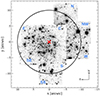 |
Fig. 1. Reconstructed I-band images of the MUSE/NFM pointings acquired in the core of M75. The circle is centered on the cluster center (red cross, from Contreras Ramos et al. 2012) and has a radius of 10″. |
MUSE/NFM datasets for M75.
The mosaic of the reconstructed I-band images from the stacking of MUSE datacubes is shown in Fig. 1. Each pointing is labeled with a name according to its position with respect to the cluster center: C, E, N, NW, S, SS, SE, and W stand for central, eastern, northern, northwestern, southern, south-southern, southeastern, and western pointing, respectively. As can be appreciated, the mosaic provides a nice and almost complete sampling of the innermost ∼7″ radial region of the cluster.
3. Analysis
For the extraction of the MUSE spectra we used the software PampelMuse (Kamann et al. 2013), which is designed to extract deblended source spectra of individual stars from observations of crowded stellar regions with integral field spectroscopy, by performing a wavelength-dependent point spread function (PSF) fitting.
3.1. The photometric catalog
PampelMuse needs in input the spectroscopic datacube and a photometric reference catalog with the coordinates of the stars in the datacube field of view, and their magnitudes. We noticed that the photometric catalog presented in Contreras Ramos et al. (2012) is not appropriate for this purpose since many bright stars are lacking because of saturation. Therefore, we decided to build a new catalog by analyzing the archive images acquired by the Hubble Space Telescope (HST) with the Wide Field Camera 3 (WFC3) secured by using the F438W and F555W filters (proposal ID: 11628, PI: Noyola).
A total of six images have been analyzed: three images in the F438W filter with an exposure time of 420 s, and three in the F555W with an exposure time of 100 s. The photometric analysis has been performed using the software DAOPHOT (Stetson 1987). Briefly, in a first step the PSF in each image is modeled by using a large subsample (∼200) of bright, isolated, and well-distributed stars. Then, a star search is performed in each image with a 5σ threshold above the background level, and the PSF model previously found is fitted to all of these identified sources. Subsequently, we created as reference a master list including all the sources measured in at least half of the images acquired with the F555W filter. Using this master list, we ran the DAOPHOT/ALLFRAME package (Stetson 1994) to force the fit of the PSF model to the location of these sources in all the other images. For each of the identified stars, the magnitude values measured in the different filters were combined using DAOMATCH and DAOMASTER. The final catalog includes the instrumental coordinates, the mean magnitude in each filter, and the photometric errors for the detected sources. The instrumental magnitudes were then calibrated to the VEGAMAG photometric system by using the appropriate aperture corrections, zero-points and the procedure reported on the HST/WFC3 website1. The instrumental positions were corrected for the effect of geometric distortions within the field of view, by applying the correction coefficients quoted in Bellini et al. (2011). Finally, the distortion-corrected positions have been placed onto the absolute coordinate system (α, δ) by cross-correlation with the Gaia DR3 catalog (Gaia Collaboration 2023).
Even in this catalog, however, a few bright stars (∼10) are saturated. To include them in the analysis, we thus performed a similar photometric analysis on two 2D MUSE images obtained by stacking the wavelength slices at 4840−4860 Å and 6060−6080 Å of each datacube. For each MUSE pointing we obtained a catalog with the instrumental positions and magnitudes of the detected stars. Then, the cross-correlation with the HST/WFC3 catalog discussed above allowed us to assign absolute coordinates and calibrated magnitudes to every MUSE star. We emphasize that we used the MUSE photometry only to recover the magnitude of the few bright stars that were saturated in the HST/WFC3 catalog. As the final reference catalog for PampelMuse, we thus adopted the HST/WFC3 catalog (which guarantees high astrometric precision and allows us to properly resolve stars even in the most crowded regions), with the addition of the MUSE measurements obtained for the few saturated sources.
In addition to the reference catalog and the datacube, PampelMuse also requires as input an analytical PSF model, which is necessary for the source deblending. We selected the MAOPPY function (Fétick et al. 2019) as PSF model, which accurately reproduces the typical double-component (core and halo) shape of the AO-corrected PSF in the MUSE/NFM observations (see Göttgens et al. 2021). Once the inputs are set, for each slice of the MUSE datacube, PampelMuse performs a PSF fitting using a subsample of stars, obtaining the wavelength dependences of the PSF parameters. At the same time, the software fits, for each slice, also the coordinate transformation from the reference catalog to the data. Then, these wavelength-dependent quantities are used to perform the deblending of all the sources present in the MUSE field of view, and extract the spectra.
3.2. The measure of radial velocities
To measure the radial velocity (RV) of the surveyed stars, we applied the same procedure described in Leanza et al. (2023, see also Pallanca et al. 2023), which uses the Doppler shifts of the calcium triplet lines (8450 − 8750 Å). The procedure needs a set of suitable synthetic spectra to be used as reference. We computed a library of synthetic spectra using the SYNTHE code (Sbordone et al. 2004; Kurucz 2005), adopting an α−enhanced chemical mixture ([α/Fe] = 0.4 dex), the cluster metallicity [Fe/H] = −1.29 dex (Carretta et al. 2009), and a set of atmospheric parameters (effective temperature and gravity) appropriate for the evolutionary stage of the targets, according to their position in the color-magnitude diagram (CMD). The spectra have been produced in the same wavelength range sampled by the observations, and convolved with a Gaussian profile to reproduce also the MUSE spectral resolution. Firstly, the observed spectra are normalized to the continuum, which is computed through a spline fitting of the spectrum in a proper wavelength range. The procedure compares the normalized observed spectra with each synthetic spectrum of the library, which is shifted in RV by steps of 0.1 km s−1 in an adequate range of RVs. For each velocity shift, and each template, the residuals between the observed spectrum and the synthetic one are computed. Then, for each target, the procedure finds the minimum standard deviation among all the residuals. This value is associated with a specific template and RV shift; therefore, the procedure derives the best-fit synthetic spectrum (hence, an estimate of temperature and gravity) and the RV of the target. The procedure computes also the signal-to-noise ratio (S/N) of the spectra as the ratio between the average of the counts and their standard deviation in the spectral range 8000 − 9000 Å. The S/N of the targets is shown by the color scale in the left panel of Fig. 2.
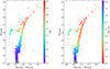 |
Fig. 2. CMD of M75 (gray dots) obtained from the HST/WFC3 photometric catalog described in Sect. 3. The large colored circles show the spectroscopic targets of the MUSE catalog (see Sect. 3.3), while the color scale in the left and right panels represents the S/N of the spectra and the RV uncertainty, respectively. |
We estimated the RV uncertainties (ϵRV) using Monte Carlo simulations. We generated ∼9000 simulated spectra with S/N between 10 and 90, and applied to these spectra the same procedure used for the observed ones, obtaining a relation to derive the RV uncertainties (for more details see Leanza et al. 2023). The errors obtained are on the order of 2 km s−1 for the brightest stars, and increase to ∼8 km s−1 for the faintest stars, as shown by the color scale of the CMD in the right panel of Fig. 2.
3.3. Final MUSE catalog
In order to obtain a consistent catalog, we checked if the RV measurements were homogeneous among the different MUSE pointings. To this aim, exploiting the several overlapping fields in our dataset, we compared the RV values measured for the stars in common between two adjacent overlapping regions, and we found offsets ranging from 2 to 4 km s−1. These offsets in the RV measurements might be introduced by variations in the wavelength calibration among the different pointings, since the MUSE observations were taken during different nights (in some cases in different months). To check the accuracy of the wavelength calibration and correct the offsets, we measured the RV from the Fraunhofer A telluric absorption bands (7570 − 7680 Å). We estimated the telluric RV for a subsample of targets with S/N > 20 by using a procedure analogous to that adopted for the determination of the star RVs. In this case, a single template spectrum was adopted for each night. We generated the appropriate synthetics for the telluric absorption spectra by using the TAPAS tool2 (Bertaux et al. 2014), setting the MUSE spectral range and resolution. For each pointing, we determined the average telluric RV, finding velocity zero-points from 0.4 km s−1 up to a maximum of 3.3 km s−1. We then subtracted the value of each pointing from all the RV measurements of the stars in that field, in order to align the different pointings. The comparison of the RV values in two overlapping pointings after the correction finally showed a good agreement within the errors.
Moreover, we used the velocity measures (v1 and v2) of the targets in common between multiple pointings and their associated errors (ϵ1 and ϵ2) to check whether the estimated RV uncertainties are reliable. If the quantity
 (1)
(1)
results in a normal distribution with unit standard deviation, the uncertainties are properly estimated (see also Kamann et al. 2016). The resulting distribution is plotted in Fig. 3 and shows that our uncertainties have been properly estimated.
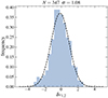 |
Fig. 3. Histogram of the values of δv1, 2 obtained from Eq. (1) for the stars with multiple exposures. The dashed black line represents the Gaussian fit to the histogram. Its standard deviation and the number of stellar pairs used are labeled at the top of the panel. |
To construct the final catalog, only stars with S/N > 10 have been considered, and for the targets with multiple exposures, the RV value was determined as the weighted mean of all the available measures, by using the individual errors as weights. The resulting MUSE catalog consists of 1872 RV measurements of individual stars. The CMD position of these stars is highlighted in Fig. 2 with large circles color-coded according to the S/N values and the RV uncertainties, in the left and right panels, respectively. Figure 4 shows the position of all the MUSE targets (gray dots and colored circles) in the plane of the sky with respect to the cluster center, while their RVs as a function of the distance from the center and their RV distribution are plotted in Fig. 5 (left panel and empty histogram in the right panel, respectively).
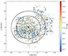 |
Fig. 4. Position of the MUSE targets in the plane of the sky, with respect to the cluster center (black cross, Contreras Ramos et al. 2012). The large colored circles mark the sample of stars that remain after the quality selection (S/N > 20 and RV error < 5 km s−1; see Sect. 4) and used for the kinematic analysis, while the gray dots indicate the rejected targets. The color scale gives the mF555W magnitude, and the two circles are centered in the cluster center and have radii of 7″ and 10″. |
4. Results
For our kinematic study we selected the (630) stars with the best RV measurements3, with S/N > 20 and RV error < 5 km s−1. The position in the plane of the sky of the selected sample is shown in Fig. 4 with large colored circles.
4.1. Systemic velocity
The black dots and the gray shaded histogram in Fig. 5 show the RV distribution of the well-measured stars. As can be appreciated, the contamination from Galactic field sources is essentially null for this field of view. To properly determine the systemic velocity (Vsys) of M75 we made the conservative choice of applying a 2σ-clipping algorithm to the selected targets, thus removing possible outliers. Assuming a Gaussian distribution of the velocities, we estimated  and its uncertainty by using a maximum-likelihood algorithm (Walker et al. 2006). The resulting value is Vsys = −189.5 ± 0.3 km s−1. This result is in full agreement with the values quoted in Baumgardt & Hilker (2018, −188.6 ± 0.9 km s−1) and Harris (1996, −189.3 ± 3.6 km s−1), while it is consistent within ∼2σ with that derived in Koch et al. (2018, −186.2 ± 1.5 km s−1).
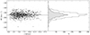 |
Fig. 5. Line-of-sight velocity distribution of M75. Left panel: RVs of the final MUSE catalog (see Sect. 3.3) plotted as a function of the distance from the cluster center. The black dots highlight the sample of the well-measured stars (i.e., those with S/N > 20 and RV error < 5 km s−1) that is used for the kinematic analysis. Right panel: empty histogram showing the number distribution of the entire RV sample, and gray histogram corresponding to the subsample of bona fide stars (black dots in the left panel). |
4.2. Systemic rotation
The internal kinematics of M75 has been little studied so far. In a previous work, Koch et al. (2018) found an indication of internal rotation in the outer region of the cluster. However, their analysis is based on a statistically poor sample (only 32 stars) of RV measurements. Taking advantage of our large dataset, here we investigated the possible presence of ordered rotation in the central regions of the system.
For the analysis of the cluster’s internal rotation, we adopted a method often used in the literature (see, e.g., Leanza et al. 2023; Pallanca et al. 2023, and references therein; see also Cote et al. 1995; Bellazzini et al. 2012, for a full description of the method). Since the proper application of the procedure requires a uniform distribution of the RV measures in the plane of the sky, we limited the analysis to the subsample of (403) stars located within 7″ from the center (corresponding to r < 1.4 rc, where rc = 4.9″ is the cluster core radius estimated in this work, see Sect. 6 and Fig. 7), thus avoiding some under-sampled regions (see Fig. 4).
The obtained results are discussed in the following and shown in Fig. 6. Following the adopted method, the RV sample is split into two subsamples by a line passing through the center of the system, and with the position angle (PA) varying counterclockwise from 0° (north) to 180° (south), in steps of 10°. The left panel of Fig. 6 shows the difference between the average velocity of the stars on each side of this line (ΔVmean), as a function of PA. This draws an approximately sinusoidal pattern, which is a signal expected in the case of ordered rotation. From the maximum/minimum of the best-fit sine function (solid red line), we derived the rotation amplitude (Arot = 0.8 ± 0.3 km s−1) as the half of this absolute value and the PA of the rotation axis (PA0 = 174 ± 3°). In the middle panel of the same figure, the black dots show the measured RVs as a function of the projected distances from the rotation axis (XR), the dashed red line is the linear fit to the data performed by means of a least square algorithm. A rotating cluster should show a highly asymmetric distribution along two diagonally opposite quadrants. Finally, the cumulative velocity distributions of the two subsamples of stars on each side of the rotation axis are shown in the right panel. A large difference between the two curves corresponds to a high probability of rotation. Therefore, to quantify the statistical significance of this difference, we used three estimators. We computed the p-value of the Kolmogorov-Smirnov (KS) probability that the RV distributions of the two subsamples are extracted from the same parent family (PKS), the t-Student probability that the two RV samples have different means (PStud), and the significance level (in units of n-σ) that the two means are different following a maximum-likelihood approach (n-σML), obtaining PKS = 0.1, PStud > 95% and n-σML = 2.9, respectively.
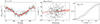 |
Fig. 6. Diagnostic diagrams of the rotation signal detected in M75, within 7″ from the cluster center. Left panel: difference between the mean RV on each side of an axis passing through the center as a function of the PA of the axis itself. The red line is the sine function that best fits the observed pattern, while the red shaded region marks the confidence level at 3σ. Central panel: distribution of the RVs referred to Vsys (Vr), as a function of the projected distances from the rotation axis (XR) in arcseconds. The value of PA0 is labeled. The dashed red line is the least square fit to the data, and the red shaded area represents the 1σ uncertainty of the linear fit. Right panel: cumulative Vr distributions for the stars with XR < 0 (solid line) and for those with XR > 0 (dotted line). The KS probability that the two subsamples are extracted from the same parent distribution is labeled. |
These results indicate a mild rotation signal in the region between 0″ and 7″, with a maximum amplitude of ∼1.0 km s−1. Although the statistical significance of this signal is not high, it is important to note that our estimate of the position angle of the rotation axis (PA0 = 174 ± 3°) is in good agreement with that found in Koch et al. (2018, PA0 = −15 ± 30°, which corresponds to 165° according to our definition of PA) using a sample of 32 stars in the radial region 20″ < r < 250″. Considering that the cluster regions explored in these two studies are complementary, we can conclude that there is a hint of ordered rotation in M75.
4.3. Velocity dispersion profile
Given a sample of individual RV measurements, the dispersion of the RV distributions observed at different radial distances from the center provides the second velocity moment profile σII(r) of the cluster. This is related to the projected velocity dispersion profile σP(r) through the following expression:  . As discussed in the previous section, the amplitude of internal rotation (if any) is very small, and we can therefore assume that the velocity dispersion is reasonably approximated by the second velocity moment (hereafter σP(r) = σII(r)).
To determine the velocity dispersion profile of M75 we divided the sample of bona fide RV measures into four concentric radial bins of increasing distance from the center, each one including more than 50 stars. We then applied a 3σ-clipping algorithm to remove the outliers, and we determined the dispersion of the remaining RV measures through a maximum-likelihood approach, by maximizing the following likelihood:
![Mathematical equation: $$ \begin{aligned} \mathrm{ln} \mathcal{L} = - \frac{1}{2}\sum _{i}^\Big [\frac{V_{\mathrm{r},i}^2}{(\sigma ^2+\epsilon _{\mathrm{v},i}^2)} + \mathrm{ln} (\sigma ^2+\epsilon _{\mathrm{v},i}^2)\Big ], \end{aligned} $$](/articles/aa/full_html/2024/08/aa50147-24/aa50147-24-eq4.gif) (2)
(2)
where Vr, i = RVi − Vsys is the RV of the ith star in the considered bin with respect to the cluster systemic velocity, ϵv, i is its corresponding error, σ is the velocity dispersion in the bin, and the summation is made over all the stars included in the bin. We implemented the likelihood using a Markov chain Monte Carlo (MCMC) approach, based on the emcee algorithm (Foreman-Mackey et al. 2013). From the posterior probability distribution function (PDF) obtained for the velocity dispersion in each bin, we derived the best-fit values of the dispersion as the PDF median, and its uncertainty from the 68% confidence interval. The velocity dispersion profile thus determined in the core of M75 is shown in the left panel of Fig. 7 (black circles) and listed in Table 2. The profile is roughly constant in the very center and starts to decrease at about 6″ from the center.
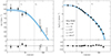 |
Fig. 7. Projected velocity dispersion and density profiles of M75. Left panel: projected velocity dispersion profile of M75 obtained from the MUSE RV measures discussed in this work (black circles). The values of the line-of-sight velocity dispersion quoted in the online repository (https://people.smp.uq.edu.au/HolgerBaumgardt/globular/) and the one obtained from Gaia proper motions (Vasiliev & Baumgardt 2021) rescaled to the distance estimated in Sect. 5 (see Table 3) are also plotted as empty circles and an empty square, respectively. The blue line corresponds to the best-fit King model derived from the simultaneous fit to this profile and the density profile shown in the right panel. The shaded regions show the 1σ uncertainty on the best fit. The dashed and dotted vertical lines mark the derived core radius (rc) and half-mass radius (rh), respectively. The bottom panel shows the residuals between the King model and the observations. Right panel: projected density profile from resolved star counts obtained by Contreras Ramos et al. (2012, black circles). The meaning of the lines, shaded region, and bottom panel is the same as in the left panel. The values of the best-fit central dimensionless potential (W0), concentration parameter (c), rc, rh, and tidal radius (rt) are labeled in the panel. |
Velocity dispersion profile of M75.
5. Distance, reddening, and age estimate
The high quality of the available HST photometric dataset offers the possibility of updated estimates of the cluster distance, reddening and age. In fact, the positions of various evolutionary sequences in the CMD of an old stellar population provide useful references to constrain these parameters through the comparison with theoretical models (see examples in Saracino et al. 2019; Cadelano et al. 2019, 2020a,b; Deras et al. 2023; Massari et al. 2023). In particular, the vertical portion of the CMD at the base of the red giant branch (RGB), and the horizontal portion of the horizontal branch (HB) are sensitive, respectively, to the color excess and the cluster distance, independently of the (old) age of the population, while the main sequence turnoff and the sub-giant branch regions are the most age-sensitive evolutionary sequences.
To determine first-guess estimates of color excess and distance, we extracted from the BaSTI-IAC database (Pietrinferni et al. 2021) a 12 Gyr old isochrone with appropriate metallicity ([Fe/H] = −1.3 dex; Carretta et al. 2009) standard helium mass fraction (Y = 0.25), and [α/Fe] = +0.4 (which is the typical value for Galactic GCs at this metallicity). We searched for the shifts in color and magnitude necessary to superpose the model to the samples of stars selected at the base of the RGB in the magnitude range 19 < mF555W < 20 and in the HB portion at 0.5 < (mF438W − mF555W) < 0.8. A reasonable reproduction of the observed loci is obtained by adopting a color excess E(B − V) = 0.16 and a distance modulus (m − M)0 = 16.7. Starting from these first-guess values, we then determined the best-fit cluster age, distance, and reddening through the isochrone fitting technique, following a Bayesian procedure similar to that used in many previous works (see, e.g., Saracino et al. 2019; Cadelano et al. 2019, 2020b; Deras et al. 2023; Massari et al. 2023). This approach consists in comparing the observed CMD with a set of isochrones, simultaneously exploring suitable grids for the age, distance modulus and color excess. We extracted a set of isochrones from the BaSTI-IAC repository (Pietrinferni et al. 2021) computed assuming the same chemical composition quoted above, and ages ranging between 9 Gyr and 15 Gyr, in steps of 0.2 Gyr. The comparison between the observed CMD and the isochrones has been performed by adopting an MCMC technique, assuming a Gaussian likelihood function (see Eqs. (2) and (3) in Cadelano et al. 2020b). To properly constrain the level of the HB, we also included a term in the likelihood function to minimize the distance in magnitude between the zero-age HB of the models and the level of the red portion of the observed HB. We used the emcee code (Foreman-Mackey et al. 2013) to sample the posterior probability distribution in the parameter space. A flat prior has been assumed for the explored age range. To convert the isochrone absolute magnitudes to the observational plane, we adopted values of the color excess and distance modulus following Gaussian prior distributions peaked at the first-guess values quoted above. To improve the definition of the main sequence turnoff and sub-giant branch evolutionary sequences in the CMD (in the magnitude range 19.5 < mF555W < 21.5), we considered only stars at distances larger than 25″ from the cluster center.
The best-fit values correspond to the 50th percentile of the posterior probability distribution of each parameter. Since we constrained the HB level and fixed the metallicity of the models, the formal 1σ uncertainties obtained from the posterior probability distributions of the MCMC are underestimated. Hence, we have included the uncertainty on the HB level in the propagation of the errors and adopted the conservative 1σ uncertainties listed below. The best-fit values of the derived quantities are E(B − V) = 0.17 ± 0.02, (m − M)0 = 16.64 ± 0.05 (corresponding to a distance of 21.3 ± 0.5 kpc), and an age of 11.0 ± 0.4 Gyr (see also Table 3). The resulting best-fit isochrone is shown in Fig. 8. Assuming a larger metallicity ([Fe/H] = −1.2 dex; see Kacharov et al. 2013), the isochrone fit slightly worsens, but it still provides values of the three parameters that are consistent with the best-fit ones within the errors. While the estimated reddening is fully consistent with that reported in the literature (Harris 1996), the distance of the cluster is slightly larger than the previous values (20.9 kpc in Harris 1996, 20.52 kpc in Baumgardt & Vasiliev 2021).
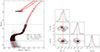 |
Fig. 8. Diagnostic plots for the determination of the distance, the reddening, and the age of M75. Left panel: CMD of M75 (gray dots) with the best-fit BaSTI isochrone computed with [Fe/H] = −1.3 dex plotted as a solid red line. The dashed red isochrones represent the uncertainties on the parameters. The black circles mark the stars used for the isochrone fitting procedure. The resulting best-fit values of color excess, distance modulus, and age are labeled. Right panel: corner plots showing the 1D and 2D projections of the posterior probability distributions for all the parameters derived from the MCMC method. The contours correspond to the 68%, 95%, and 99% confidence levels. |
Parameters of M75 determined in this work.
6. Discussion and conclusions
In this paper we have presented a new result of the MIKiS survey: the first kinematic exploration of the central regions of M75 (NGC 6864), a GC orbiting the outer halo of the Milky Way. By using a set of AO-corrected MUSE/NFM observations, we obtained a sample of ∼1900 RV measurements of individual stars located within 16″ (∼3 rc) from the cluster center. From a subsample of 630 well-measured stars (i.e., with MUSE spectra with S/N > 20 and with RV uncertainties smaller than 5 km s−1), we determined the systemic velocity of the cluster (Vsys = −189.5 ± 0.3 km s−1) and the innermost portion (r < 16″) of its velocity dispersion profile. By taking advantage of the high photometric quality of the HST/WFC3 catalog, we also determined updated estimates of the cluster distance, reddening, and age (see Table 3).
By using a set of single-mass, spherical, isotropic, and non-rotating King models (King 1966)4, we simultaneously fit the velocity dispersion profile obtained by combining the one derived in this work with literature values (see the left panel of Fig. 7) and the projected density profile obtained from the resolved star counts in Contreras Ramos et al. (2012). The approximation of single-mass and non-rotating models is legitimated by the facts that both profiles were obtained from samples of stars with approximately the same mass (main sequence turnoff and giant stars) and that the rotation signal is negligible in this system (see Sect. 4.2).
The best-fit solution was determined using an MCMC method through the emcee algorithm (Foreman-Mackey et al. 2013). We assumed a χ2 likelihood and uniform priors on the parameters of the fit (i.e., the King concentration parameter, c, the core radius, rc, the value of the central density, and the central velocity dispersion, σ0). For each parameter, the 50th percentile of the PDF was adopted as the best-fit value, while the 16th and 84th percentiles were used to determine the 1σ uncertainty. The fitting procedure provides a best-fit King model characterized by W0 = 7.85 ± 0.1, concentration c = 1.79 ± 0.03, core radius  , half-mass radius
  , tidal radius
  , and central velocity dispersion σ0 = 8.8 ± 0.3 km s−1. Figure 7 shows the resulting best-fit King model (solid blue lines) overplotted on the observed velocity dispersion and density profiles (left and right panels, respectively). The bottom panels show the residuals between the model and the observations. The best-fit values and the uncertainties of each parameter are listed in Table 3.
The value of the central velocity dispersion estimated in this work is significantly smaller than those quoted in Koch et al. (2018,  km s−1) and in Baumgardt & Hilker (2018, σ0 = 11.8 km s−1, which has since been updated to 12.3 km s−1 in the online version). However, the literature values are both extrapolated from the fit to observational data that are confined to the cluster’s outer regions, while, for the first time, the central portion of the velocity dispersion profile is directly constrained by observations in this work. In particular, Koch et al. (2018) fit a Plummer model (see their Eq. (3)) to a sample of just 32 stars located between ∼20″ and 250″ from the center, while Baumgardt & Hilker (2018) used N-body simulations and a velocity dispersion profile with the innermost radial bin located at ∼70″ from the center (see the empty circles in Fig. 7). It is also worth keeping in mind that our analysis is mainly based on RGB stars that are slightly more massive (∼0.8 M⊙) than the average cluster stars (∼0.3 M⊙), while the central velocity dispersion estimated by Baumgardt & Hilker (2018) from N-body simulations is weighted by stellar masses. Taking the effects of energy equipartition and mass segregation into account, this could partially explain the smaller value estimated in this work. Indeed, the analyses conducted so far clearly suggest that M75 is a highly dynamically evolved stellar system. The central relaxation time (log trc/yr = 8.0; Lanzoni et al. 2016) compared to the cluster age (11 Gyr; see Sect. 5) indicates that the system has undergone several relaxations so far. In addition, the large value of the BSS segregation level (the
  parameter) empirically confirms the high level of dynamical evolution and central mass segregation in this cluster (see Lanzoni et al. 2016; Ferraro et al. 2023a). Hence, RGB stars are more centrally segregated than the average, and their central velocity dispersion is lower than the mass-weighted value.
M75 can be well approximated by a single-mass, spherical, isotropic, and non-rotating King model (King 1966). Under this assumption, the total mass of the system can be estimated from the value of σ0 following Eq. (3) in Majewski et al. (2003, see also Richstone & Tremaine 1986): M = 1.66 rcμ/β, where μ is a polynomial function of the King concentration parameter (see Eq. (8) in Djorgovski 1993), and  . The resulting total mass is M = 2.5 ± 0.2 × 10⁵ M⊙; the uncertainty was estimated through Monte Carlo simulations (see Leanza et al. 2022; Pallanca et al. 2023). This value is a factor of two smaller than the value derived in Baumgardt & Hilker (2018, 5.86 ± 1.24 × 10⁵ M⊙), mainly due to the significant difference in the values of σ0, as well as the different assumptions (e.g., from Sect. 5, we adopted a distance of 21.3 kpc, while Baumgardt & Hilker 2018 used 20.5 kpc) and the different methods used in the two works.
Finally, using the selected sample of MUSE RVs, we investigated the systemic rotation in the innermost region of the cluster (r < 7″, corresponding to r < 1.4 rc). We find just a weak hint of rotation (Arot ∼ 1 km s−1), with a position angle of the rotation axis of PA0 = 174 ± 3°. It is intriguing to note that the value of PA0 obtained in the present paper is fully consistent with that of the rotation signal detected by Koch et al. (2018) in the outer regions. Thus, despite the limitations of the two samples and the low statistical significance of both detections, there is now a stronger hint of internal rotation in M75 that deserves further investigation.
The sample of bona fide RV measures with the corresponding errors is publicly available at: http://www.cosmic-lab.eu/Cosmic-Lab/MIKiS_Survey.html
The King models (King 1966) are a single-parameter family of dynamical models, meaning that their shape is univocally determined by the dimensionless parameter W0, which is proportional to the gravitational potential at the center of the system, or alternatively, by the concentration parameter c ≡ log(rt/r0), where rt and r0 are the tidal and the King radii of the model, respectively. Other characteristic parameters of the cluster structure are the core radius rc and the half-mass radius rh.
Acknowledgments
This work is part of the project Cosmic-Lab at the Physics and Astronomy Department “A. Righi” of the Bologna University (http://www.cosmic-lab.eu/Cosmic-Lab/Home.html).
References
- Arsenault, R., Madec, P.-Y., Hubin, N., et al. 2008, Proc. SPIE, 7015, 701524 [NASA ADS] [CrossRef] [Google Scholar]
- Bacon, R., Accardo, M., Adjali, L., et al. 2010, Proc. SPIE, 7735, 773508 [Google Scholar]
- Bailyn, C. D. 1995, ARA&A, 33, 133 [NASA ADS] [CrossRef] [Google Scholar]
- Baumgardt, H., & Hilker, M. 2018, MNRAS, 478, 1520 [Google Scholar]
- Baumgardt, H., & Vasiliev, E. 2021, MNRAS, 505, 5957 [NASA ADS] [CrossRef] [Google Scholar]
- Bellazzini, M., Bragaglia, A., Carretta, E., et al. 2012, A&A, 538, A18 [NASA ADS] [CrossRef] [EDP Sciences] [Google Scholar]
- Bellini, A., Anderson, J., & Bedin, L. R. 2011, PASP, 123, 622 [CrossRef] [Google Scholar]
- Bertaux, J. L., Lallement, R., Ferron, S., et al. 2014, A&A, 564, A46 [NASA ADS] [CrossRef] [EDP Sciences] [Google Scholar]
- Billi, A., Ferraro, F. R., Mucciarelli, A., et al. 2023, ApJ, 956, 124 [NASA ADS] [CrossRef] [Google Scholar]
- Cadelano, M., Ransom, S. M., Freire, P. C. C., et al. 2018, ApJ, 855, 125 [Google Scholar]
- Cadelano, M., Ferraro, F. R., Istrate, A. G., et al. 2019, ApJ, 875, 25 [NASA ADS] [CrossRef] [Google Scholar]
- Cadelano, M., Chen, J., Pallanca, C., et al. 2020a, ApJ, 905, 63 [NASA ADS] [CrossRef] [Google Scholar]
- Cadelano, M., Saracino, S., Dalessandro, E., et al. 2020b, ApJ, 895, 54 [NASA ADS] [CrossRef] [Google Scholar]
- Cadelano, M., Pallanca, C., Dalessandro, E., et al. 2023, A&A, 679, L13 [NASA ADS] [CrossRef] [EDP Sciences] [Google Scholar]
- Carretta, E., Bragaglia, A., Gratton, R., et al. 2009, A&A, 508, 695 [NASA ADS] [CrossRef] [EDP Sciences] [Google Scholar]
- Contreras Ramos, R., Ferraro, F. R., Dalessandro, E., et al. 2012, ApJ, 748, 91 [NASA ADS] [CrossRef] [Google Scholar]
- Cote, P., Welch, D. L., Fischer, P., et al. 1995, ApJ, 454, 788 [NASA ADS] [CrossRef] [Google Scholar]
- Crociati, C., Valenti, E., Ferraro, F. R., et al. 2023, ApJ, 951, 17 [NASA ADS] [CrossRef] [Google Scholar]
- Dalessandro, E., Lanzoni, B., Ferraro, F. R., et al. 2008, ApJ, 677, 1069 [NASA ADS] [CrossRef] [Google Scholar]
- Dalessandro, E., Salaris, M., Ferraro, F. R., et al. 2013a, MNRAS, 430, 459 [NASA ADS] [CrossRef] [Google Scholar]
- Dalessandro, E., Ferraro, F. R., Massari, D., et al. 2013b, ApJ, 778, 135 [NASA ADS] [CrossRef] [Google Scholar]
- Dalessandro, E., Massari, D., Bellazzini, M., et al. 2014, ApJ, 791, L4 [NASA ADS] [CrossRef] [Google Scholar]
- Dalessandro, E., Lapenna, E., Mucciarelli, A., et al. 2016, ApJ, 829, 77 [NASA ADS] [CrossRef] [Google Scholar]
- Dalessandro, E., Raso, S., Kamann, S., et al. 2021, MNRAS, 506, 813 [CrossRef] [Google Scholar]
- Dalessandro, E., Crociati, C., Cignoni, M., et al. 2022, ApJ, 940, 170 [NASA ADS] [CrossRef] [Google Scholar]
- Deras, D., Cadelano, M., Ferraro, F. R., et al. 2023, ApJ, 942, 104 [CrossRef] [Google Scholar]
- Deras, D., Cadelano, M., Lanzoni, B., et al. 2024, A&A, 681, A38 [NASA ADS] [CrossRef] [EDP Sciences] [Google Scholar]
- Dresbach, F., Massari, D., Lanzoni, B., et al. 2022, ApJ, 928, 47 [NASA ADS] [CrossRef] [Google Scholar]
- Djorgovski, S. 1993, ASP Conf. Ser., 50, 373 [NASA ADS] [Google Scholar]
- Ferraro, F. R., Fusi Pecci, F., & Buonanno, R. 1992, MNRAS, 256, 376 [NASA ADS] [CrossRef] [Google Scholar]
- Ferraro, F. R., Paltrinieri, B., Fusi Pecci, F., et al. 1997, ApJ, 484, L145 [Google Scholar]
- Ferraro, F. R., Paltrinieri, B., Rood, R. T., et al. 1999, ApJ, 522, 983 [CrossRef] [Google Scholar]
- Ferraro, F. R., Possenti, A., D’Amico, N., et al. 2001, ApJ, 561, L93 [NASA ADS] [CrossRef] [Google Scholar]
- Ferraro, F. R., Sills, A., Rood, R. T., et al. 2003, ApJ, 588, 464 [NASA ADS] [CrossRef] [Google Scholar]
- Ferraro, F. R., Dalessandro, E., Mucciarelli, A., et al. 2009a, Nature, 462, 483 [Google Scholar]
- Ferraro, F. R., Beccari, G., Dalessandro, E., et al. 2009b, Nature, 462, 1028 [NASA ADS] [CrossRef] [Google Scholar]
- Ferraro, F. R., Lanzoni, B., Dalessandro, E., et al. 2012, Nature, 492, 393 [Google Scholar]
- Ferraro, F. R., Massari, D., Dalessandro, E., et al. 2016, ApJ, 828, 75 [NASA ADS] [CrossRef] [Google Scholar]
- Ferraro, F. R., Lanzoni, B., Raso, S., et al. 2018a, ApJ, 860, 36 [NASA ADS] [CrossRef] [Google Scholar]
- Ferraro, F. R., Mucciarelli, A., Lanzoni, B., et al. 2018b, ApJ, 860, 50 [NASA ADS] [CrossRef] [Google Scholar]
- Ferraro, F. R., Mucciarelli, A., Lanzoni, B., et al. 2018c, The Messenger, 172, 18 [NASA ADS] [Google Scholar]
- Ferraro, F. R., Lanzoni, B., Dalessandro, E., et al. 2019, Nat. Astron., 3, 1149 [NASA ADS] [CrossRef] [Google Scholar]
- Ferraro, F. R., Lanzoni, B., & Dalessandro, E. 2020, Rendiconti Lincei. Scienze Fisiche e Naturali, 31, 19 [NASA ADS] [CrossRef] [Google Scholar]
- Ferraro, F. R., Pallanca, C., Lanzoni, B., et al. 2021, Nat. Astron., 5, 311 [Google Scholar]
- Ferraro, F. R., Lanzoni, B., Vesperini, E., et al. 2023a, ApJ, 950, 145 [NASA ADS] [CrossRef] [Google Scholar]
- Ferraro, F. R., Mucciarelli, A., Lanzoni, B., et al. 2023b, Nat. Commun., 14, 2584 [NASA ADS] [CrossRef] [Google Scholar]
- Fétick, R. J. L., Fusco, T., Neichel, B., et al. 2019, A&A, 628, A99 [NASA ADS] [CrossRef] [EDP Sciences] [Google Scholar]
- Foreman-Mackey, D., Hogg, D. W., Lang, D., et al. 2013, PASP, 125, 306 [NASA ADS] [CrossRef] [Google Scholar]
- Freudling, W., Romaniello, M., Bramich, D. M., et al. 2013, A&A, 559, A96 [NASA ADS] [CrossRef] [EDP Sciences] [Google Scholar]
- Gaia Collaboration (Vallenari, A., et al.) 2023, A&A, 674, A1 [NASA ADS] [CrossRef] [EDP Sciences] [Google Scholar]
- Göttgens, F., Kamann, S., Baumgardt, H., et al. 2021, MNRAS, 507, 4788 [CrossRef] [Google Scholar]
- Harris, W. E. 1996, AJ, 112, 1487 [Google Scholar]
- Kacharov, N., Koch, A., & McWilliam, A. 2013, A&A, 554, A81 [NASA ADS] [CrossRef] [EDP Sciences] [Google Scholar]
- Kamann, S., Wisotzki, L., & Roth, M. M. 2013, A&A, 549, A71 [NASA ADS] [CrossRef] [EDP Sciences] [Google Scholar]
- Kamann, S., Husser, T.-O., Brinchmann, J., et al. 2016, A&A, 588, A149 [NASA ADS] [CrossRef] [EDP Sciences] [Google Scholar]
- King, I. R. 1966, AJ, 71, 64 [Google Scholar]
- Koch, A., Hanke, M., & Kacharov, N. 2018, A&A, 616, A74 [NASA ADS] [CrossRef] [EDP Sciences] [Google Scholar]
- Kurucz, R. L. 2005, Mem. Soc. Astron. It. Suppl., 8, 14 [Google Scholar]
- Ibata, R., Bellazzini, M., Chapman, S. C., et al. 2009, ApJ, 699, L169 [NASA ADS] [CrossRef] [Google Scholar]
- Lanzoni, B., Dalessandro, E., Ferraro, F. R., et al. 2007, ApJ, 668, L139 [NASA ADS] [CrossRef] [Google Scholar]
- Lanzoni, B., Ferraro, F. R., Dalessandro, E., et al. 2010, ApJ, 717, 653 [Google Scholar]
- Lanzoni, B., Mucciarelli, A., Origlia, L., et al. 2013, ApJ, 769, 107 [NASA ADS] [CrossRef] [Google Scholar]
- Lanzoni, B., Ferraro, F. R., Alessandrini, E., et al. 2016, ApJ, 833, L29 [NASA ADS] [CrossRef] [Google Scholar]
- Lanzoni, B., Ferraro, F. R., Mucciarelli, A., et al. 2018a, ApJ, 861, 16 [NASA ADS] [CrossRef] [Google Scholar]
- Lanzoni, B., Ferraro, F. R., Mucciarelli, A., et al. 2018b, ApJ, 865, 11 [NASA ADS] [CrossRef] [Google Scholar]
- Lanzoni, B., Ferraro, F. R., Dalessandro, E., et al. 2019, ApJ, 887, 176 [NASA ADS] [CrossRef] [Google Scholar]
- Leanza, S., Pallanca, C., Ferraro, F. R., et al. 2022, ApJ, 929, 186 [NASA ADS] [CrossRef] [Google Scholar]
- Leanza, S., Pallanca, C., Ferraro, F. R., et al. 2023, ApJ, 944, 162 [NASA ADS] [CrossRef] [Google Scholar]
- Libralato, M., Bellini, A., van der Marel, R. P., et al. 2018, ApJ, 861, 99 [CrossRef] [Google Scholar]
- Massari, D., Mucciarelli, A., Ferraro, F. R., et al. 2014, ApJ, 791, 101 [NASA ADS] [CrossRef] [Google Scholar]
- Massari, D., Aguado-Agelet, F., Monelli, M., et al. 2023, A&A, 680, A20 [NASA ADS] [CrossRef] [EDP Sciences] [Google Scholar]
- Majewski, S. R., Skrutskie, M. F., Weinberg, M. D., et al. 2003, ApJ, 599, 1082 [Google Scholar]
- Miocchi, P., Lanzoni, B., Ferraro, F. R., et al. 2013, ApJ, 774, 151 [Google Scholar]
- Origlia, L., Ferraro, F. R., Fusi Pecci, F., et al. 1997, A&A, 321, 859 [NASA ADS] [Google Scholar]
- Origlia, L., Ferraro, F. R., Fusi Pecci, F., et al. 2002, ApJ, 571, 458 [NASA ADS] [CrossRef] [Google Scholar]
- Origlia, L., Ferraro, F. R., Bellazzini, M., et al. 2003, ApJ, 591, 916 [CrossRef] [Google Scholar]
- Origlia, L., Rich, R. M., Ferraro, F. R., et al. 2011, ApJ, 726, L20 [CrossRef] [Google Scholar]
- Origlia, L., Massari, D., Rich, R. M., et al. 2013, ApJ, 779, L5 [NASA ADS] [CrossRef] [Google Scholar]
- Origlia, L., Mucciarelli, A., Fiorentino, G., et al. 2019, ApJ, 871, 114 [NASA ADS] [CrossRef] [Google Scholar]
- Pallanca, C., Dalessandro, E., Ferraro, F. R., et al. 2010, ApJ, 725, 1165 [CrossRef] [Google Scholar]
- Pallanca, C., Dalessandro, E., Ferraro, F. R., et al. 2013, ApJ, 773, 122 [NASA ADS] [CrossRef] [Google Scholar]
- Pallanca, C., Ransom, S. M., Ferraro, F. R., et al. 2014, ApJ, 795, 29 [NASA ADS] [CrossRef] [Google Scholar]
- Pallanca, C., Beccari, G., Ferraro, F. R., et al. 2017, ApJ, 845, 4 [NASA ADS] [CrossRef] [Google Scholar]
- Pallanca, C., Lanzoni, B., Ferraro, F. R., et al. 2021, ApJ, 913, 137 [NASA ADS] [CrossRef] [Google Scholar]
- Pallanca, C., Leanza, S., Ferraro, F. R., et al. 2023, ApJ, 950, 138 [NASA ADS] [CrossRef] [Google Scholar]
- Paresce, F., de Marchi, G., & Ferraro, F. R. 1992, Nature, 360, 46 [NASA ADS] [CrossRef] [Google Scholar]
- Pietrinferni, A., Hidalgo, S., Cassisi, S., et al. 2021, ApJ, 908, 102 [NASA ADS] [CrossRef] [Google Scholar]
- Pooley, D., Lewin, W. H. G., Anderson, S. F., et al. 2003, ApJ, 591, L131 [NASA ADS] [CrossRef] [Google Scholar]
- Pryor, C., & Meylan, G. 1993, ASP Conf. Ser., 50, 357 [NASA ADS] [Google Scholar]
- Ransom, S. M., Hessels, J. W. T., Stairs, I. H., et al. 2005, Science, 307, 892 [NASA ADS] [CrossRef] [PubMed] [Google Scholar]
- Raso, S., Libralato, M., Bellini, A., et al. 2020, ApJ, 895, 15 [NASA ADS] [CrossRef] [Google Scholar]
- Richstone, D. O., & Tremaine, S. 1986, AJ, 92, 72 [NASA ADS] [CrossRef] [Google Scholar]
- Saracino, S., Dalessandro, E., Ferraro, F. R., et al. 2015, ApJ, 806, 152 [NASA ADS] [CrossRef] [Google Scholar]
- Saracino, S., Dalessandro, E., Ferraro, F. R., et al. 2019, ApJ, 874, 86 [Google Scholar]
- Sbordone, L., Bonifacio, P., Castelli, F., et al. 2004, Mem. Soc. Astron. It. Suppl., 5, 93 [Google Scholar]
- Stetson, P. B. 1987, PASP, 99, 191 [Google Scholar]
- Stetson, P. B. 1994, PASP, 106, 250 [Google Scholar]
- Ströbele, S., La Penna, P., Arsenault, R., et al. 2012, Proc. SPIE, 8447, 844737 [CrossRef] [Google Scholar]
- Valenti, E., Ferraro, F. R., & Origlia, L. 2010, MNRAS, 402, 1729 [NASA ADS] [CrossRef] [Google Scholar]
- Vasiliev, E., & Baumgardt, H. 2021, MNRAS, 505, 5978 [NASA ADS] [CrossRef] [Google Scholar]
- Walker, M. G., Mateo, M., Olszewski, E. W., et al. 2006, AJ, 131, 2114 [Google Scholar]
- Weilbacher, P. M., Palsa, R., Streicher, O., et al. 2020, A&A, 641, A28 [NASA ADS] [CrossRef] [EDP Sciences] [Google Scholar]
All Tables
All Figures
|
Fig. 1. Reconstructed I-band images of the MUSE/NFM pointings acquired in the core of M75. The circle is centered on the cluster center (red cross, from Contreras Ramos et al. 2012) and has a radius of 10″. |
| In the text | |
|
Fig. 2. CMD of M75 (gray dots) obtained from the HST/WFC3 photometric catalog described in Sect. 3. The large colored circles show the spectroscopic targets of the MUSE catalog (see Sect. 3.3), while the color scale in the left and right panels represents the S/N of the spectra and the RV uncertainty, respectively. |
| In the text | |
|
Fig. 3. Histogram of the values of δv1, 2 obtained from Eq. (1) for the stars with multiple exposures. The dashed black line represents the Gaussian fit to the histogram. Its standard deviation and the number of stellar pairs used are labeled at the top of the panel. |
| In the text | |
|
Fig. 4. Position of the MUSE targets in the plane of the sky, with respect to the cluster center (black cross, Contreras Ramos et al. 2012). The large colored circles mark the sample of stars that remain after the quality selection (S/N > 20 and RV error < 5 km s−1; see Sect. 4) and used for the kinematic analysis, while the gray dots indicate the rejected targets. The color scale gives the mF555W magnitude, and the two circles are centered in the cluster center and have radii of 7″ and 10″. |
| In the text | |
|
Fig. 5. Line-of-sight velocity distribution of M75. Left panel: RVs of the final MUSE catalog (see Sect. 3.3) plotted as a function of the distance from the cluster center. The black dots highlight the sample of the well-measured stars (i.e., those with S/N > 20 and RV error < 5 km s−1) that is used for the kinematic analysis. Right panel: empty histogram showing the number distribution of the entire RV sample, and gray histogram corresponding to the subsample of bona fide stars (black dots in the left panel). |
| In the text | |
|
Fig. 6. Diagnostic diagrams of the rotation signal detected in M75, within 7″ from the cluster center. Left panel: difference between the mean RV on each side of an axis passing through the center as a function of the PA of the axis itself. The red line is the sine function that best fits the observed pattern, while the red shaded region marks the confidence level at 3σ. Central panel: distribution of the RVs referred to Vsys (Vr), as a function of the projected distances from the rotation axis (XR) in arcseconds. The value of PA0 is labeled. The dashed red line is the least square fit to the data, and the red shaded area represents the 1σ uncertainty of the linear fit. Right panel: cumulative Vr distributions for the stars with XR < 0 (solid line) and for those with XR > 0 (dotted line). The KS probability that the two subsamples are extracted from the same parent distribution is labeled. |
| In the text | |
|
Fig. 7. Projected velocity dispersion and density profiles of M75. Left panel: projected velocity dispersion profile of M75 obtained from the MUSE RV measures discussed in this work (black circles). The values of the line-of-sight velocity dispersion quoted in the online repository (https://people.smp.uq.edu.au/HolgerBaumgardt/globular/) and the one obtained from Gaia proper motions (Vasiliev & Baumgardt 2021) rescaled to the distance estimated in Sect. 5 (see Table 3) are also plotted as empty circles and an empty square, respectively. The blue line corresponds to the best-fit King model derived from the simultaneous fit to this profile and the density profile shown in the right panel. The shaded regions show the 1σ uncertainty on the best fit. The dashed and dotted vertical lines mark the derived core radius (rc) and half-mass radius (rh), respectively. The bottom panel shows the residuals between the King model and the observations. Right panel: projected density profile from resolved star counts obtained by Contreras Ramos et al. (2012, black circles). The meaning of the lines, shaded region, and bottom panel is the same as in the left panel. The values of the best-fit central dimensionless potential (W0), concentration parameter (c), rc, rh, and tidal radius (rt) are labeled in the panel. |
| In the text | |
|
Fig. 8. Diagnostic plots for the determination of the distance, the reddening, and the age of M75. Left panel: CMD of M75 (gray dots) with the best-fit BaSTI isochrone computed with [Fe/H] = −1.3 dex plotted as a solid red line. The dashed red isochrones represent the uncertainties on the parameters. The black circles mark the stars used for the isochrone fitting procedure. The resulting best-fit values of color excess, distance modulus, and age are labeled. Right panel: corner plots showing the 1D and 2D projections of the posterior probability distributions for all the parameters derived from the MCMC method. The contours correspond to the 68%, 95%, and 99% confidence levels. |
| In the text | |
Current usage metrics show cumulative count of Article Views (full-text article views including HTML views, PDF and ePub downloads, according to the available data) and Abstracts Views on Vision4Press platform.
Data correspond to usage on the plateform after 2015. The current usage metrics is available 48-96 hours after online publication and is updated daily on week days.
Initial download of the metrics may take a while.