| Issue |
A&A
Volume 691, November 2024
|
|
|---|---|---|
| Article Number | A94 | |
| Number of page(s) | 22 | |
| Section | Galactic structure, stellar clusters and populations | |
| DOI | https://doi.org/10.1051/0004-6361/202451054 | |
| Published online | 01 November 2024 | |
A 3D view of multiple populations’ kinematics in Galactic globular clusters
1
INAF – Astrophysics and Space Science Observatory Bologna,
Via Gobetti 93/3,
40129
Bologna,
Italy
2
Dipartimento di Fisica e Astronomia,
Via Gobetti 93/2,
40129
Bologna,
Italy
3
Department of Astronomy, Indiana University,
Swain West, 727 E. 3rd Street,
IN
47405
Bloomington,
USA
★ Corresponding author; This email address is being protected from spambots. You need JavaScript enabled to view it.
Received:
10
June
2024
Accepted:
2
September
2024
Abstract
We present the first 3D kinematic analysis of multiple stellar populations (MPs) in a representative sample of 16 Galactic globular clusters (GCs). For each GC in the sample, we studied the MP line-of-sight, plane-of-the-sky and 3D rotation, and velocity distribution anisotropy. The differences between first-population (FP) and second-population (SP) kinematic patterns were constrained by means of parameters specifically defined to provide a global measure of the relevant physical quantities and to enable a meaningful comparison among different clusters. Our analysis provides the first observational description of the MP kinematic properties and of the path they follow during their long-term dynamical evolution. In particular, we find evidence of differences between the rotation of MPs along all velocity components with the SP preferentially rotating faster than the FP. The difference between the rotation strength of MPs is anticorrelated with the cluster dynamical age. We also observe that FPs are characterized by isotropic velocity distributions at any dynamical age probed by our sample. On the contrary, the velocity distribution of SP stars is found to be radially anisotropic in dynamically young clusters and isotropic at later evolutionary stages. The comparison with a set of numerical simulations shows that these observational results are consistent with the long-term evolution of clusters forming with an initially more centrally concentrated and more rapidly rotating SP subsystem. We discuss the possible implications these findings have on our understanding of MP formation and early evolution.
Key words: techniques: photometric / techniques: radial velocities / stars: abundances / Hertzsprung-Russell and C-M diagrams / stars: kinematics and dynamics / globular clusters: general
© The Authors 2024
 Open Access article, published by EDP Sciences, under the terms of the Creative Commons Attribution License (https://creativecommons.org/licenses/by/4.0), which permits unrestricted use, distribution, and reproduction in any medium, provided the original work is properly cited.
This article is published in open access under the Subscribe to Open model. This email address is being protected from spambots. You need JavaScript enabled to view it. to support open access publication.
1 Introduction
Globular clusters (GCs) exhibit intrinsic star-to-star variations in their light -element content. In fact, while some GC stars have the same light-element abundances as field stars with the same metallicity (first population or generation – FP), others show enhanced N and Na along with depleted C and O abundances (second population or generation – SP). The manifestation of such light-element inhomogeneities is referred to as multiple stellar populations (MPs; see Bastian & Lardo 2018 and Gratton et al. 2019 for a review of the subject).
Light-element abundance variations can have an impact on both the stellar structures (as in the case of He, for example) and atmospheres (as for Na, O, C, and N), and they can therefore produce a broadening or splitting of different evolutionary sequences in color-magnitude-diagrams (CMDs) when appropriate filter combinations are used (Piotto et al. 2007; Sbordone et al. 2011; Dalessandro et al. 2011; Monelli et al. 2013; Piotto et al. 2015; Niederhofer et al. 2017; Cadelano et al. 2023). It is well established that the MP phenomenon is (almost) ubiquitous among massive stellar clusters. In fact, it has been shown that nearly all massive (>104 M⊙; e.g., Dalessandro et al. 2014; Piotto et al. 2015; Milone et al. 2017; Bragaglia et al. 2017) and relatively old (>1.5–2 Gyr; Martocchia et al. 2018b; Cadelano et al. 2022) GCs host MPs. In addition, MPs are observed in GC systems in any environment where they have been properly searched for. They are regularly found in the Magellanic Clouds’ stellar clusters (Mucciarelli et al. 2009; Dalessandro et al. 2016), in GCs in dwarf galaxies such as Fornax (Larsen et al. 2012, 2018) and Sagittarius (e.g., Sills et al. 2019), and in the M31 GC system (Schiavon et al. 2013; Nardiello et al. 2018). There are strong indications (though indirect) that they are ubiquitous in stellar clusters in massive elliptical galaxies (e.g., Chung et al. 2011).
MPs are believed to form during the very early epochs of GC formation and evolution (10–100 Myr; see Martocchia et al. 2018a; Nardiello et al. 2015 and Saracino et al. 2020 for direct observational constraints) and a number of scenarios have been proposed over the years to describe the sequence of physical events and mechanisms involved in their formation. We can schematically group them in two main categories. One includes multi-epoch formation models, which predict that MPs form during multiple (at least two) events of star formation and typically invoke self-enrichment processes, in which the SP forms out of the ejecta of relatively massive FP stars (e.g., Decressin et al. 2007; D’Ercole et al. 2008; de Mink et al. 2009; D’Antona et al. 2016). The second category includes models where MPs form simultaneously and SPs are able to accrete gas eventually during their pre-main sequence phases (e.g., Bastian et al. 2013; Gieles et al. 2018). However, independently of the specific differences, all models proposed so far have their own caveats and face serious problems in reproducing some or all the available observations. As a matter of fact, we still lack a self-consistent explanation of the physical processes at the basis of MP formation (e.g., see Bastian & Lardo 2018; Gratton et al. 2019).
Understanding the kinematical and structural properties of MPs can provide new insights into the early epochs of GC formation and evolution. In fact, most formation models suggest that MPs form with different structural and kinematic properties. Differences between the FP and the SP kinematics can be either imprinted at the time of SP formation (see, e.g., Bekki 2010; Lacchin et al. 2022) or emerge during a cluster’s evolution as a consequence of the initial differences between the FP and SP spatial distributions (see e.g., Tiongco et al. 2019; Vesperini et al. 2021; Sollima 2021). Although the primordial structural and kinematic differences between FP and SP stars are expected to be gradually erased during GC long-term dynamical evolution (e.g., Vesperini et al. 2013; Hénault-Brunet et al. 2015; Tiongco et al. 2019; Vesperini et al. 2021; Sollima 2021), some clusters are expected to still retain some memory of these initial differences. Indeed, Dalessandro et al. (2019) measured the difference in the spatial distributions of FP and SP stars for a large sample of massive Galactic and Magellanic Clouds clusters homogeneously observed with the HST. The authors found that the differences between the FP and SP spatial distributions generally follow the evolutionary sequence expected for the long-term dynamical evolution of clusters forming with an initially more centrally concentrated SP subsystem (see also Leitinger et al. 2023; Onorato et al. 2023; Cadelano et al. 2024).
Spatial distributions alone can provide only a partial picture of the dynamical properties of MPs, and further key constraints on the possible formation and dynamical paths of MPs are expected to be hidden in their kinematic properties. Because of the technical limitations to deriving kinematic information for large and significant samples of resolved stars in dense environments, most of the information available so far has been obtained using HST proper motions (PMs) and ESO/VLT MUSE line-of-sight (LOS) velocities sampling relatively small portions of the cluster and focusing typically on the innermost regions. In a few particularly well-studied systems, MPs have been found to show different degrees of orbital anisotropy (e.g., Richer et al. 2013; Bellini et al. 2015; Libralato et al. 2023) and possibly different rotation amplitudes (e.g., Cordero et al. 2017; Kamann et al. 2020; Cordoni et al. 2020; Dalessandro et al. 2021a; Martens et al. 2023). In other cases, however, no significant differences between the MP kinematic properties have been observed (see, e.g., Milone et al. 2018; Cordoni et al. 2020; Libralato et al. 2019; Szigeti et al. 2021; Martens et al. 2023), and, as a consequence, the emerging internal kinematic results describe a pretty heterogeneous picture.
To move forward in our understanding of MP kinematic properties and their possible implications on GC formation, it is fundamental to perform a systematic and homogeneous study of clusters sampling a wide range of dynamical ages and including the analysis of the clusters’ outer regions, which are expected to retain some memory of the primordial structural and kinematic differences for longer timescales. As a first step in this direction, we performed for the first time a self-consistent study of the 3D kinematics of MPs in a representative sample of Galactic GCs for which it is virtually possible to sample their entire radial extension. This study has the additional advantage of overcoming the typical limitations connected with projection effects, which typically arise when LOS or plane-of-the-sky velocities (i.e., PMs) are used independently, possibly hampering the detection of the actual differences between the MP kinematic properties (see, e.g., the discussion concerning these issues in Tiongco et al. 2019).
The paper is structured as follows. In Sec. 2 the adopted sample and the observational database are presented. In Sec. 3 we describe the kinematic analysis along the three velocity components, while in Sec. 4 we present the approach adopted for the study of the morphological properties of MPs. In Sects. 5 and 6 we present the main observational results along with a detailed comparison to dynamical simulations, and in Sec. 7 we compare them with the literature. In Sec. 8 we summarize our findings and discuss their possible implications in the context of massive clusters formation and early evolution.
2 Sample definition and observational datasets
The analysis presented in this paper targets 16 Galactic GCs. In detail, the sample includes all clusters analyzed by Ferraro et al. (2018) and Lanzoni et al. (2018a,b) in the context of the ESO/VLT Multi Instrument Kinematic Survey of Galactic GCs (MIKiS), except NGC 362 as it lacks near-UV photometric data needed for the study of MPs (see Sec. 2.2 for details). We added NGC 104 (47 Tuc) to the target list as it is a massive, relatively close, and well-studied GC, which can be useful for comparative analysis. We also included NGC 6362, for which we secured a large kinematic dataset in Dalessandro et al. (2018b, 2021a), NGC 6089 (M 80) and NGC 6205 (M 13), as they have been found to show interesting kinematic properties in a previous analysis by Cordero et al. (2017) and Kamann et al. (2020). Table 1 summarizes some useful properties of the targets, such as distances, structural properties, age, relaxation times, and kinematic sample sizes. The selected clusters are representative of the overall Galactic GC population as they properly encompass the cluster’s dynamically-sensitive parameter space, spanning a wide range of central densities and concentrations, different stages of dynamical evolution, and different environmental conditions. They are also more massive than M > 104 M⊙ and relatively close to the Earth (within ~16 kpc), thus providing data with good signal-to-noise ratios (S/Ns) for a large sample of stars.
2.1 Kinematic database
The analysis performed in this work is based on two main kinematic datasets securing LOS velocities (RVs) and PMs for hundreds (or thousands in a few cases – Table 1) of red giant branch stars (RGBs) in each GC. For 12 out of 16 GCs, most of the adopted LOS RVs were obtained using ESO/VLT KMOS and FLAMES data acquired as part of the MIKiS survey. We refer the reader to Ferraro et al. (2018) for details on the overall observational strategy and data analysis. MIKiS LOS RVs were then complemented by those from the publicly available catalog of Baumgardt et al. (2019) to improve the sampling of the external regions of the target clusters. All LOS RVs used for 47 Tuc come from the Baumgardt et al. (2019) catalog. For NGC 6362, M 80, and M 13, the LOS RVs were obtained using ESO/VLT MUSE and FLAMES data (Cordero et al. 2017; Dalessandro et al. 2018b, 2021a; Kamann et al. 2020).
For each of the investigated GCs, astrometric information, namely absolute PMs ![Mathematical equation: $\[\left(\mu_\alpha^*, \mu_\delta\right)\]$](/articles/aa/full_html/2024/11/aa51054-24/aa51054-24-eq1.png) and relative errors, were retrieved from the ESA/Gaia DR3 (Gaia Collaboration 2023) archive out to the clusters’ tidal radius. Only stars with ruwe < 1.31 were then used for the kinematic analysis.
and relative errors, were retrieved from the ESA/Gaia DR3 (Gaia Collaboration 2023) archive out to the clusters’ tidal radius. Only stars with ruwe < 1.31 were then used for the kinematic analysis.
Properties of the 16 GCs analyzed in the present work.
2.2 Photometric dataset, membership selection, and differential reddening correction
We used the wide-field catalogs published by Stetson et al. (2019) including the U, B, V, R, and I bands to identify MPs in the target GCs (see Sec. 2.3). While these data are seeing-limited and can suffer from incompleteness in the crowded central regions, they have similar spatial resolution to the kinematic LOS RVs dataset. In addition, they are typically not affected by saturation problems, and therefore they maximize the number of bright stars in common with the kinematic samples. The photometric catalogs were cross-matched with the kinematic ones based on their absolute coordinates (α, δ) and using the cross-correlation tool CataXcorr2. For each cluster in the sample, the final catalog includes all stars in common between Gaia and the photometric catalogs. A fraction (typically larger than ~60% along the RGB) of these stars also has LOS RVs and is therefore suited to a full 3D analysis (see Table 1).
To separate likely cluster members from field interlopers, we selected stars whose PMs are within 2σ of the cluster systemic velocity (adopted from Vasiliev & Baumgardt 2021), where σ is the standard deviation of the observed ![Mathematical equation: $\[\left(\mu_\alpha^*, \mu_\delta\right)\]$](/articles/aa/full_html/2024/11/aa51054-24/aa51054-24-eq2.png) distribution of RGB stars. We verified that, for the clusters in our sample, reasonable variations of the adopted cluster membership selection criteria do not have a significant impact on the main results of the kinematic analysis. As an example, Fig. 1 shows the PM distribution of 47 Tuc stars along with the (U, U-I) and (U, CU,B,I -where CU,B,I = (U − B) − (B − I); Monelli et al. 2013) CMDs for both selected cluster stars and field interlopers. Figure 2 shows the distributions of the velocities along the LOS, the PM radial (RAD), and PM tangential (TAN) components as a function of the cluster-centric distance for likely member RGB stars of the same cluster. It is worth mentioning here that the kinematic catalogs obtained from the MIKiS survey already rely on the cluster membership selection performed by Ferraro et al. (2018) and Lanzoni et al. (2018a,b), which is based on both the LOS RV and [Fe/H] distributions (we refer the reader to those papers for further details).
distribution of RGB stars. We verified that, for the clusters in our sample, reasonable variations of the adopted cluster membership selection criteria do not have a significant impact on the main results of the kinematic analysis. As an example, Fig. 1 shows the PM distribution of 47 Tuc stars along with the (U, U-I) and (U, CU,B,I -where CU,B,I = (U − B) − (B − I); Monelli et al. 2013) CMDs for both selected cluster stars and field interlopers. Figure 2 shows the distributions of the velocities along the LOS, the PM radial (RAD), and PM tangential (TAN) components as a function of the cluster-centric distance for likely member RGB stars of the same cluster. It is worth mentioning here that the kinematic catalogs obtained from the MIKiS survey already rely on the cluster membership selection performed by Ferraro et al. (2018) and Lanzoni et al. (2018a,b), which is based on both the LOS RV and [Fe/H] distributions (we refer the reader to those papers for further details).
Available magnitudes were then corrected for differential reddening by using the approach described in Dalessandro et al. (2018c) (see also Cadelano et al. 2020). In short, differential reddening was estimated by using likely member stars selected in a magnitude range typically going from the RGB-bump level down to about one magnitude below the cluster turn-off. Using these stars, a mean ridge line (MRL) was defined in the (B, B-I) CMD. Then, for all stars within 3σ (where σ is the color spread around the MRL), the geometric distance from the MRL (ΔX) was computed. For each star in the catalog, differential reddening was then obtained as the mean of the ΔX values of the 30 nearest (in space) selected stars. ΔX was then transformed into differential reddening δE(B − V) using Eq. (1) from Dalessandro et al. (2018c), which was properly modified to account for the different extinction coefficients for the adopted filters. Differential reddening corrections turn out to be relatively small (<0.1mag) for most GCs in the sample, with the most critical cases being NGC 3201 and NGC 5927, for which we find δE(B − V) values larger than ~0.2 mag.
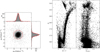 |
Fig. 1 Selection of likely cluster member stars for the GC 47 Tuc. On the left, the vector-point diagram obtained using Gaia DR3 PMs is shown along with the distribution of stars along the |
![Mathematical equation: $\[\mu_\alpha^*\]$](/articles/aa/full_html/2024/11/aa51054-24/aa51054-24-eq3.png)
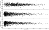 |
Fig. 2 LOS, RAD, and TAN velocity distributions of likely member stars of the GC 47 Tuc as a function of the cluster-centric distance. All velocities are shown with respect to the cluster systemic velocity along the corresponding component. |
2.3 MP classification
Starting from the sample of likely member stars and differential reddening corrected magnitudes, we identified MPs along the RGB by using their distribution in the (U, CU,B,I) CMD (Fig. 3). It has been shown that this color combination is very effective to identify MPs along the RGB with different C and N (and possibly He) abundances (Sbordone et al. 2011; Monelli et al. 2013). RGB stars were verticalized in the (U, CU,B,I) CMD with respect to two fiducial lines on the blue and red edges of the RGB, calculated as the 5th and 95th percentiles of the color distribution in different magnitude bins (Fig. 3 – see, e.g., Dalessandro et al. 2018a,c; Onorato et al. 2023 and Cadelano et al. 2023, for similar implementations of the same technique). In the resulting verticalized color distribution (![Mathematical equation: $\[\Delta_{C_{U, B, I}}\]$](/articles/aa/full_html/2024/11/aa51054-24/aa51054-24-eq4.png) ; right panel in Fig. 3), stars on the red (blue) side are expected to be N-poor (-rich), that is FP (SP). We ran a two-component Gaussian mixture modeling3 (GMM) analysis on the resulting
; right panel in Fig. 3), stars on the red (blue) side are expected to be N-poor (-rich), that is FP (SP). We ran a two-component Gaussian mixture modeling3 (GMM) analysis on the resulting ![Mathematical equation: $\[\Delta_{C_{U, B, I}}\]$](/articles/aa/full_html/2024/11/aa51054-24/aa51054-24-eq5.png) distribution, thus assigning a probability of belonging to the FP and SP subpopulations to each star. Stars with a probability of belonging to one of the two subpopulations larger than 50% were then flagged as FPs or SPs. Figure 3 shows the result of the MP identification and separation for the GC 47 Tuc. While this approach may introduce a few uncertainties and over-simplifications in the MP classification as we are not directly deriving light-element chemical abundances, it secures statistically large samples of stars with MP tagging that are hard to obtain using only spectroscopic data.
distribution, thus assigning a probability of belonging to the FP and SP subpopulations to each star. Stars with a probability of belonging to one of the two subpopulations larger than 50% were then flagged as FPs or SPs. Figure 3 shows the result of the MP identification and separation for the GC 47 Tuc. While this approach may introduce a few uncertainties and over-simplifications in the MP classification as we are not directly deriving light-element chemical abundances, it secures statistically large samples of stars with MP tagging that are hard to obtain using only spectroscopic data.
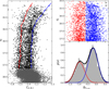 |
Fig. 3 MP identification and selection for the case of 47 Tuc. Left panel: (U, CU,B,I) CMD of likely 47 Tuc member stars. RGB stars adopted for the kinematic analysis are highlighted in black. The blue and red curves are the fiducial lines adopted to verticalize the color distribution. Right panels: top panel displays verticalized color distribution of RGB stars, while the bottom panel shows the corresponding histograms. The red and blue curves represent the two best-fit Gaussians for the FP and SP, respectively, while the solid black curve is their sum. |
3 Kinematic analysis
For each cluster in the sample we first analyzed the kinematic properties in terms of velocity dispersion, rotation, and anisotropy profiles for the LOS and plane-of-the-sky components separately (Sects. 3.1 and 3.2); then, for the fraction of stars for which all velocity components are available, we performed a full 3D study (Sect. 3.3). We adopted the cluster centers reported by Goldsbury et al. (2010). All velocities were corrected for perspective effects induced by the clusters’ systemic motions by using the equations reported in van Leeuwen (2009) and following the approach already adopted in Dalessandro et al. (2021b) and Della Croce et al. (2023).
3.1 1D velocity dispersion and rotation profiles
To characterize the kinematic properties of the clusters in the sample and of their subpopulations, we adopted the Bayesian approach described in Cordero et al. (2017) (see also Dalessandro et al. 2018b), which is based on the use of a discrete fitting technique to compare simple kinematic models (including a radial dependence of the rotational amplitude and velocity dispersion of the cluster) with individual radial velocities. We stress that this is a purely kinematic approach aimed at searching for relative differences among different clusters and sub-populations, and it is not aimed at providing a self-consistent dynamical description of each system.
The likelihood function for the radial velocities of individual stars depends on our assumptions about the formal descriptions of the rotation and velocity dispersion radial variations. For the velocity dispersion profile we assumed the functional form of the Plummer model (Plummer 1911), which is simply defined by its central velocity dispersion σ0 and its scale radius a:
![Mathematical equation: $\[\sigma^2(R)=\frac{\sigma_0^2}{\sqrt{1+R^2 / a^2}},\]$](/articles/aa/full_html/2024/11/aa51054-24/aa51054-24-eq6.png) (1)
(1)
where R is the projected distance from the center of the cluster. We adopted the same formal description for all velocity components. For the rotation curve, we assumed cylindrical rotation and adopted the functional form expected for stellar systems undergoing violent relaxation during their early phases of evolution (Lynden-Bell 1967):
![Mathematical equation: $\[V_{\text {rot}} \sin i\left(X_{\mathrm{PA}_0}\right)=\frac{2 A_{\text {rot}}}{R_{\text {peak}}} \frac{X_{\mathrm{PA}_0}}{1+\left(X_{\mathrm{PA}_0} / R_{\text {peak }}\right)^2},\]$](/articles/aa/full_html/2024/11/aa51054-24/aa51054-24-eq7.png) (2)
(2)
![Mathematical equation: $\[\mu_{\text {TAN }}=\frac{2 V_{\text {peak }}}{R_{\text {peak }}} \frac{R}{1+\left(R / R_{\text {peak }}\right)^2},\]$](/articles/aa/full_html/2024/11/aa51054-24/aa51054-24-eq8.png) (3)
(3)
for the LOS (Eq. (2)) and TAN (Eq. (3)) velocity components, respectively. In Eq. (2), Vrotsini represents the projection of the rotational amplitude along the LOS velocity component at a projected distance ![Mathematical equation: $\[X_{\mathrm{PA}_0}\]$](/articles/aa/full_html/2024/11/aa51054-24/aa51054-24-eq9.png) from the rotation axis. Arot is the peak rotational amplitude occurring at the projected distance Rpeak from the cluster center. We defined the rotation axis position angle (PA) as increasing anti-clockwise in the plane of the sky from north (PA = 0°) to east (PA = 90°). Since the inclination of the rotation axis is unknown, Vrotsini represents a lower limit to the actual rotational amplitude. As an extreme case, if the rotation axis is aligned with the line of sight, the rotation would be in the plane of the sky. In Eq. (3), Vpeak represents the maximum (in an absolute sense) of the mean motion in the TAN component.
from the rotation axis. Arot is the peak rotational amplitude occurring at the projected distance Rpeak from the cluster center. We defined the rotation axis position angle (PA) as increasing anti-clockwise in the plane of the sky from north (PA = 0°) to east (PA = 90°). Since the inclination of the rotation axis is unknown, Vrotsini represents a lower limit to the actual rotational amplitude. As an extreme case, if the rotation axis is aligned with the line of sight, the rotation would be in the plane of the sky. In Eq. (3), Vpeak represents the maximum (in an absolute sense) of the mean motion in the TAN component.
The fit of the kinematic quantities was performed by using the emcee4 (Foreman-Mackey et al. 2013) implementation of the Markov chain Monte Carlo (MCMC) sampler, which provides the posterior probability distribution function (PDFs) for σ0, a, Arot, and PA0. For each quantity, the 50th, 16th, and 84th percentiles of the PDF distributions were adopted as the best-fit values and relative errors, respectively. We assumed a Gaussian likelihood and flat priors on each of the investigated parameters within a reasonably wide range of values. It is important to note that in general, since the analysis is based on the conditional probability of a velocity measurement given the position of a star, our fitting procedure is not biased by the spatial sampling of the stars in the different clusters and subsamples. However, the kinematic properties are better constrained in regions that are better sampled (i.e., more stars with available kinematic information).
As a sanity check and comparison, we also derived the velocity dispersion and rotation profiles by splitting the surveyed areas in a set of concentric annuli, whose width was chosen as a compromise between a good radial sampling and a statistically significant number of stars. In this case, the analysis was limited radially within a maximum distance from the center of the clusters to guarantee a symmetric coverage of the field of view. The adopted limiting distance varies from one cluster to the other depending on the photometric and kinematic dataset field-of-view limits (Sec. 2.3). While this approach requires the splitting of the sample in concentric radial bins, whose number and width are at least partially arbitrary and can potentially have an impact on the final results, it has the advantage of avoiding any assumption on the model description of the velocity dispersion and rotation profiles.
In each radial bin, the velocity dispersion was computed by following the maximum-likelihood approach described by Pryor & Meylan (1993). The method is based on the assumption that the probability of finding a star with a velocity of υi and error εi at a projected distance from the cluster center Ri can be approximated as
![Mathematical equation: $\[p\left(v_i, \epsilon_i, R_i\right)=\frac{1}{2 \pi \sqrt{\sigma^2+\epsilon_i^2}} \exp \frac{\left(v_i-v_0\right)^2}{-2\left(\sigma^2+\epsilon_i^2\right)},\]$](/articles/aa/full_html/2024/11/aa51054-24/aa51054-24-eq10.png) (4)
(4)
where υ0 and σ are the systemic velocity and the intrinsic dispersion profile of the cluster along the three components (i.e., LOS, RAD, and TAN), respectively.
As for the rotation along the LOS component, we used the method fully described in Bellazzini et al. (2012) and adopted in the previous papers of our group (e.g., Ferraro et al. 2018; Lanzoni et al. 2018a; Dalessandro et al. 2021a; Leanza et al. 2022). In brief, we considered a line passing through the cluster center with the position angle varying from −90° to 90° in steps of 10°. For each value of PA, such a line splits the observed sample in two. If the cluster is rotating along the line of sight, we expect to find a value of PA that maximizes the difference between the median RVs of the two sub-samples, since one component is mostly approaching and the other is receding with respect to the observer. Moving PA from this value has the effect of gradually decreasing the difference in the median RV. Hence, the appearance of a coherent sinusoidal behavior as a function of PA is a signature of rotation, and its best-fit sine function provides an estimate of the rotation amplitude (Arot) and the position angle of the cluster rotation axis (PA0). For the plane-of-the-sky rotation, we used the variation of the mean values within each radial bin of the tangential velocity component with respect to the systematic motion.
Examples of the results obtained with both the Bayesian and maximum-likelihood analyses are shown in Figs. 4 and 5 for the MPs of the GC 47 Tuc. For all clusters in the sample, we find a good agreement between the discrete and binned analysis; however, in the following we adopt the best-fit results (and errors) obtained with the Bayesian approach. Table A.1 reports the best-fit values and relative errors for the most relevant quantities along both the LOS and plane of the sky for both the FP and SP.
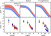 |
Fig. 4 Velocity dispersion profiles of MPs in 47Tuc. Bottom panels: observed velocity dispersion profiles along the LOS, radial, and tangential velocity components by using a maximum-likelihood approach on binned data. Upper panels: best-fit velocity dispersion profiles as obtained using the Bayesian analysis on discrete velocities described in Sec. 3.1. |
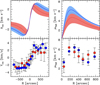 |
Fig. 5 Same as Fig. 4, but for rotation profiles along LOS (left panel) and TAN (right panel) components for MPs in 47 Tuc. |
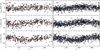 |
Fig. 7 Distribution of the three velocity components as a function of the position angle for MPs in 47 Tuc. Left and right panels refer to the FP and SP subpopulations, respectively. The solid lines show the best-fitting trend in all panels. |
3.2 Anisotropy profiles
We adopted a modified version of the Osipkov-Merrit (Osipkov 1979; Merritt 1985) model to provide a formal description of the velocity anisotropy profile for each cluster and subpopulation (see Aros et al., in prep. for further details). This model is isotropic in the cluster center, and it becomes increasingly anisotropic for R > ra (where ra is the anisotropy radius). Our anisotropy description includes two additional parameters, which are the “outer” anisotropy value (β∞) and the truncation radius (rt):
![Mathematical equation: $\[\beta(R)=\frac{\beta_{\infty} R^2}{\left(R^2+r_a\right)^2}\left(1-\frac{R}{r_t}\right).\]$](/articles/aa/full_html/2024/11/aa51054-24/aa51054-24-eq11.png) (5)
(5)
β∞ defines how radial or tangentially biased the velocity anisotropy profile is for R≫ra, and rt is the radius at which the velocity anisotropy becomes isotropic again. In practice, we adopt rt as the Jacobi radius of the cluster.
Following the same approach adopted for the velocity dispersion and rotation, we performed an MCMC fit of the anisotropy profiles (see results in Table A.1) using the individual stellar velocities along the radial and tangential components (μRAD and μTAN, respectively) and assuming a Gaussian likelihood in which the best-fit velocity dispersion along the radial direction σRAD can be described through a Plummer profile (see Eq. (1)) and the velocity dispersion along the tangential direction is simply given by ![Mathematical equation: $\[\sigma_{\mathrm{TAN}}^2=[1-\beta(R)] \sigma_{\mathrm{RAD}}^2\]$](/articles/aa/full_html/2024/11/aa51054-24/aa51054-24-eq12.png) . It is important to stress that this assumption is only adopted for the best-fit anisotropy parameter derivation, while we generally consider those derived through the independent fitting of σRAD and σTAN discussed in Sec. 3.1 as best-fit velocity dispersion profiles. For the binned analysis, the anisotropy profiles were obtained directly from the RAD and TAN velocity dispersion values obtained in Sec. 3.1. Figure 6 shows an example of the best-fit anisotropy profile for the MPs of 47 Tuc.
. It is important to stress that this assumption is only adopted for the best-fit anisotropy parameter derivation, while we generally consider those derived through the independent fitting of σRAD and σTAN discussed in Sec. 3.1 as best-fit velocity dispersion profiles. For the binned analysis, the anisotropy profiles were obtained directly from the RAD and TAN velocity dispersion values obtained in Sec. 3.1. Figure 6 shows an example of the best-fit anisotropy profile for the MPs of 47 Tuc.
3.3 Full 3D analysis
To perform a full 3D analysis, we used the kinematic sample of member stars with both LOS RVs and Gaia PMs after quality selection (see Sec. 2.1). We also limited the analysis to the same radial extension adopted for the binned maximum-likelihood analysis (Sec. 3.1).
We followed the approach described in Sollima et al. (2019), which has the advantage of constraining a cluster full-rotation pattern by estimating the inclination angle of the rotation axis (i) with respect to the line of sight, the position angle of the rotation axis (θ0), and the rotation velocity amplitude (A), by means of a model-independent analysis. We refer the reader to that paper for a full description of the method. Here, we only report the main ingredients and assumptions.
In a real cluster, the angular velocity is expected to be a function of the distance from the rotation axis (see, e.g., Eqs. (1) and (2)). To account for such a dependence in a rigorous way, a rotating model should be fit to the data. However, to perform a model-independent analysis, we considered an average projected rotation velocity with amplitude A3D, which has been assumed to be independent of the distance from the cluster center. While of course this represents a crude approximation of the rotation patterns expected in GCs and provides a rough average of the actual rotation amplitude, it is important to stress that it does not introduce any bias in the estimation of θ0 and i.
A3D, i, and θ0 were derived by solving the equations describing the rotation projection along the LOS (VLOS) and those perpendicular (V⊥) and parallel (V|) to the rotation axes (see Eq. (2) in Sollima et al. 2019). While the velocity component perpendicular to the rotation axis has a dependence on stellar positions within the cluster along the line of sight, we neglected it in our analysis. In fact, we note that the dependence on the stellar distance along the line of sight does not affect the mean trend of the perpendicular velocity component, but it can only introduce an additional spread on its distribution. We assumed that i varies in the range 0° < i < 90° with respect to the line of sight and the position angle in the 0° < θ0 < 360° range. θ0 grows counterclockwise from north to east, and A3D is positive for clockwise rotation in the plane of the sky. Following the approach already adopted for the 1D analysis, we derived the best-fit rotation amplitudes, position and inclination angles, and relative errors by maximizing the likelihood function reported in Eq. (3) of Sollima et al. (2019) using the MCMC algorithm emcee. Best-fit results are reported in Table A.1. Figure 7 shows the result of the best-fit analysis along the three velocity components for the FP and SP subpopulations of 47 Tuc.
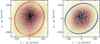 |
Fig. 8 2D density maps of stars selected in the GC 47 Tuc for kinematic analysis. FPs are shown in the left panel, while SPs in the right panel. Overplotted to the density distributions are the best-fit ellipses derived as described in Sect. 4. |
4 Morphological analysis: MP ellipticity
We inferred the ellipticity of the MPs by constructing the so-called shape tensor (Zemp et al. 2011), which is defined by the following equation:
![Mathematical equation: $\[S_{\mathrm{ij}} \equiv \frac{\sum_{\mathrm{k}} m_{\mathrm{k}}\left(R_{\mathrm{k}}\right)_{\mathrm{i}}\left(R_{\mathrm{k}}\right)_{\mathrm{j}}}{\sum_{\mathrm{k}} m_{\mathrm{k}}},\]$](/articles/aa/full_html/2024/11/aa51054-24/aa51054-24-eq13.png) (6)
(6)
where Rk and mk are the projected distance from the cluster center and the mass of the k-th star, within the i-th and j-th elements of the shape tensor grid. For the purpose of this study, we assumed that all stars have the same mass. This assumption is well justified, as the adopted sample consists of RGB stars (the same as that used for the kinematic analysis), whose mass variations for a given cluster are expected to be ~0.02M⊙, depending on the metallicity.
The shape tensor was computed starting from a spherical grid, whose nodes are the stellar radial distribution’s 10th, 50th, and 90th percentiles. We adopted an iterative procedure for each bin during which the shape tensor is initially constructed from spherical distances. After that, with (w0; w1) being the eigenvalues (with w0 > w1) and (υ0; υ1) the respective eigenvectors of the shape tensor, it follows (Zemp et al. 2011) that
![Mathematical equation: $\[\epsilon=1-\frac{w_1}{w_0} \quad \text { and } \quad \mathrm{PA}=\arctan \frac{v_{0, \mathrm{y}}}{v_{0, \mathrm{x}}}.\]$](/articles/aa/full_html/2024/11/aa51054-24/aa51054-24-eq14.png) (7)
(7)
The particle coordinates were then rotated by the angle −PA, and distances to the center were defined by means of the circularized distance
![Mathematical equation: $\[R_{\mathrm{ell}} \equiv \sqrt{x^{\prime 2}+\frac{y^{\prime 2}}{\epsilon^2}},\]$](/articles/aa/full_html/2024/11/aa51054-24/aa51054-24-eq15.png) (8)
(8)
where (x′; y′) are the rotated, locally Cartesian coordinates of the stars.
Finally, stars were binned in the new coordinate system according to the initial grid, and the shape tensor was computed using Rell instead of R. Such a procedure was then iterated until a relative precision of 5% on the axis ratio was reached. Best-fit ellipticity values and relative errors were obtained by means of a bootstrapping analysis. In detail, the shape tensor was computed 1000 times for each cluster by randomly selecting a subsample including only 90% of the stars at each time. The values corresponding to the 50th percentile of the distribution of all the ε values was then adopted as best-fit, while the errors correspond to the 16th and 84th percentiles. As an example, Fig. 8 shows the result of the analysis for the MPs in 47 Tuc, while Table A.1 reports the best-fit values for each GC and subpopulation.
5 Results: rotation
To obtain quantitative and homogeneous estimates of the possible kinematic differences among MPs, to follow their evolution, and eventually to compare the results obtained for all GCs in the sample with theoretical models and dynamical simulations, we introduced a few simple parameters described in detail in the following. These parameters are meant to incorporate, in a meaningful way, all the main relevant physical quantities at play in a single value. The general approach of our analysis is not to focus on the detection of specific and particularly significant kinematic differences of specific targets, but rather to compare the general kinematic behaviors described by MPs in all targets in the sample in the most effective way.
A description about the approach adopted to quantify the possible impact of the intrinsically limited statistical kinematic samples and of their incompleteness on the final results is discussed in Appendix B. Here, we briefly stress that the main effects are not on the derived best-fit values, but rather on their uncertainties. While the main focus of the following sections is the MP kinematics, we also analyzed the entire sample of stars with kinematic information (hereafter labeled TOT) for comparison with previous works, and we present the main results in Appendix C.
5.1 Observations
To measure the rotation differences between the SP and FP subpopulations for all clusters in the sample for both the LOS and TAN velocity components, we introduced a parameter, hereafter referred to as α. It is defined as the area subtended by the ratio between the best-fit rotation velocity profile and the best-fit velocity dispersion profile for each subpopulation in a cluster (Sec. 3.1) after rescaling the cluster-centric distance to the value of the peak (Rα) of such a distribution:
![Mathematical equation: $\[\alpha^X=\int_0^1 V_{\mathrm{rot}}\left(R_1\right) / \sigma\left(R_1\right) \mathrm{d} R_{\mathrm{l}},\]$](/articles/aa/full_html/2024/11/aa51054-24/aa51054-24-eq16.png) (9)
(9)
where Vrot(Rl) and σ(Rl) can either refer to the LOS or the TAN velocity components, Rl is the cluster-centric distance normalized to the Rα, and the index X refers to the different subpopulations (i.e., FP or SP). Derived values are reported in Table 2.
This parameter has the advantage of providing a robust measure of the relative strength of the rotation signal over the disordered motion at any radial range without making any assumption about the underlying star or mass distribution. By construction α depends on the considered cluster-centric distance and therefore a meaningful cluster-to-cluster comparison requires that the parameter is measured over equivalent radial portions in every system. As shown in a number of numerical studies (see, e.g., Hénault-Brunet et al. 2015; Tiongco et al. 2019), dynamical evolution is expected to smooth out primordial kinematic and structural differences in the innermost regions first and then in the cluster’s outskirts. Therefore, capturing rotation differences between MPs requires a compromise between probing a fairly wide radial coverage in order to trace regions where kinematic differences should be present for a longer time and sampling distances from the cluster center where rotation is more prominent. With this in mind, we decided to measure α within Rα. We also verified that the adoption of different radial selections does not have a significant impact on the overall relative distribution of α values. Errors on α were obtained by propagating the posterior probability distributions obtained from the MCMC analysis for the best-fit rotation and velocity dispersion profiles’ derivation (see Sec. 3.1). Differences between SP and FP kinematic patterns are constrained simply by (αSP − αFP). With such a definition, a more rapidly rotating SP yields positive values of (αSP − αFP).
Along similar lines, we defined a parameter to describe the 3D rotation:
![Mathematical equation: $\[\omega_{3 D}^X=\left(A_{3 \mathrm{D}} / \sigma_0^{3 \mathrm{D}}\right) /\left(R_{\mathrm{m}} / R_{\mathrm{h}}\right),\]$](/articles/aa/full_html/2024/11/aa51054-24/aa51054-24-eq17.png) (10)
(10)
where ![Mathematical equation: $\[\sigma_0^{3 \mathrm{D}}\]$](/articles/aa/full_html/2024/11/aa51054-24/aa51054-24-eq18.png) represents the 3D central velocity dispersion and it is defined as the quadratic average of the σ0 values obtained for the three velocity components (i.e., LOS, TAN, and RAD - Sec. 3.1); Rm is the average cluster-centric distance of stars for which we have tridimensional velocity measures, and Rh is the system half-light radius (from Harris 1996). Here, Rh is adopted as a meaningful radial normalization factor to secure a direct comparison among different GCs attaining significantly different projected radial extension. In the assumption of a pure solid-body rotation, ω3D would represent the best-fit angular rotation. Values derived for each cluster and sub-population are reported in Table 2. As for the 1D analysis, the introduction of ω3D is primarily meant to provide a direct and reliable characterization of the 3D rotation based only on quantities that are directly derived from the observations. Differences in the 3D rotation of SP and FP are given by
represents the 3D central velocity dispersion and it is defined as the quadratic average of the σ0 values obtained for the three velocity components (i.e., LOS, TAN, and RAD - Sec. 3.1); Rm is the average cluster-centric distance of stars for which we have tridimensional velocity measures, and Rh is the system half-light radius (from Harris 1996). Here, Rh is adopted as a meaningful radial normalization factor to secure a direct comparison among different GCs attaining significantly different projected radial extension. In the assumption of a pure solid-body rotation, ω3D would represent the best-fit angular rotation. Values derived for each cluster and sub-population are reported in Table 2. As for the 1D analysis, the introduction of ω3D is primarily meant to provide a direct and reliable characterization of the 3D rotation based only on quantities that are directly derived from the observations. Differences in the 3D rotation of SP and FP are given by ![Mathematical equation: $\[\left(\omega_{3 \mathrm{D}}^{\mathrm{SP}}-\omega_{3 \mathrm{D}}^{\mathrm{FP}}\right)\]$](/articles/aa/full_html/2024/11/aa51054-24/aa51054-24-eq19.png) , which yields positive values for a more rapidly rotating SP.
, which yields positive values for a more rapidly rotating SP.
Several works have shown that the rotation strength observed in GCs is primarily shaped by their dynamical age, with dynamically young systems typically showing the larger degree of rotation (e.g., Fabricius et al. 2014; Bianchini et al. 2018; Kamann et al. 2018; Sollima et al. 2019). We used Nh = tage/trh as a proxy of the clusters’ dynamical ages. We adopted the half-mass relaxation time (trh) values reported by Harris (1996) and ages derived by Dotter et al. (2010) for all clusters except for NGC 1904, for which we used the age inferred by Dalessandro et al. (2013).
In Fig. C.1, we show the distribution of the α values (along both the LOS and TAN velocity components) and of ω3D as a function of Nh for the TOT population. In general, we find a very good agreement with previous analyses (e.g., Bianchini et al. 2018; Kamann et al. 2018; Baumgardt et al. 2019; Sollima et al. 2019) in terms of correlation between cluster rotation strength and dynamical age, thus further strengthening the idea that the present-day cluster rotation is the relic of that imprinted at the epoch of cluster formation, and that it has since progressively dissipated via two-body relaxation (Einsel & Spurzem 1999; Hong et al. 2013; Tiongco et al. 2017; Livernois et al. 2022; Kamlah et al. 2022). Interestingly, such an agreement also provides an independent assessment of the reliability of the adopted kinematic parameters.
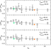
In Figs. 9–11, we show the distributions of α (for both the LOS and PM components) and of ω3D as a function of Nh for both SP and FP stars (bottom and middle panels). Interestingly, a number of common patterns can be highlighted in the three figures. First, we note that in a large fraction of clusters (up to ~50%) both FP and SP show evidence of non-negligible rotation. Second, both subpopulations show evidence of anticorrelation with Nh in all three analyzed velocity components, with dynamically young clusters being characterized by a larger rotation strength. This behavior turns out to be more prominent when the PM and 3D analyses are considered. This is somehow expected as PMs are less affected than the LOS velocities by the smoothing introduced by the superposition of stars located at different cluster-centric distances and attaining different rotation velocities. In addition, the 3D analysis accounts for any rotation axis inclination and projection effects. Finally, we observe that for all velocity components, in dynamically young clusters the SP is characterized by larger α and ω3D values (i.e., more rapid rotation) than that observed for the FP at similar Nh, and it shows a more rapid decline than the FP as a function of Nh. In fact, a Spearman correlation test gives a probability Pspear larger than ~99% of correlations between (αSP)PM or ![Mathematical equation: $\[\omega_{3 \mathrm{D}}^{\mathrm{SP}}\]$](/articles/aa/full_html/2024/11/aa51054-24/aa51054-24-eq20.png) and Nh, while probabilities are smaller when either the LOS component or the FP is considered. We note here that by using the approach described in Curran (2015) we have verified that the results of the Spearman rank correlation tests performed in our analysis and reported in the following are robust against possible outliers and errors associated with the adopted kinematic parameters.
and Nh, while probabilities are smaller when either the LOS component or the FP is considered. We note here that by using the approach described in Curran (2015) we have verified that the results of the Spearman rank correlation tests performed in our analysis and reported in the following are robust against possible outliers and errors associated with the adopted kinematic parameters.
To better highlight such a differential behavior, the upper panels of Figs. 9–11 show the difference between the rotation strength of the SP and FP as given by (αSP − αFP) and ![Mathematical equation: $\[\left(\omega_{3 \mathrm{D}}^{\mathrm{SP}}-\omega_{3 \mathrm{D}}^{\mathrm{FP}}\right)\]$](/articles/aa/full_html/2024/11/aa51054-24/aa51054-24-eq117.png) . Admittedly, neither (αSP − αFP) nor
. Admittedly, neither (αSP − αFP) nor ![Mathematical equation: $\[\left(\omega_{3 \mathrm{D}}^{\mathrm{SP}}-\omega_{3 \mathrm{D}}^{\mathrm{FP}}\right)\]$](/articles/aa/full_html/2024/11/aa51054-24/aa51054-24-eq118.png) show striking variations in the dynamical age range sampled by the target clusters (2 < Nh < 25). In fact, Spearman rank correlation tests give probabilities of correlation of Pspear ~ 90% (~95% in the 3D case). Interestingly, however, a negative trend between the rotation strength differences and Nh is consistently observed in all velocity components. In fact, both (αSP − αFP) and
show striking variations in the dynamical age range sampled by the target clusters (2 < Nh < 25). In fact, Spearman rank correlation tests give probabilities of correlation of Pspear ~ 90% (~95% in the 3D case). Interestingly, however, a negative trend between the rotation strength differences and Nh is consistently observed in all velocity components. In fact, both (αSP − αFP) and ![Mathematical equation: $\[\left(\omega_{3 \mathrm{D}}^{\mathrm{SP}}-\omega_{3 \mathrm{D}}^{\mathrm{FP}}\right)\]$](/articles/aa/full_html/2024/11/aa51054-24/aa51054-24-eq119.png) show positive values for dynamically young GCs, and then they progressively approach zero for dynamically older clusters, meaning that FP and SP rotate at the same velocity. The good agreement between the results obtained in the three analyses definitely supports the fact that there is a real correlation between the SP and FP rotation strength differences and Nh, and that SP generally shows a more rapid rotation than the FP at dynamically young ages. These results represent the first observational evidence of the link between MP rotation patterns and clusters’ long-term dynamical evolution.
show positive values for dynamically young GCs, and then they progressively approach zero for dynamically older clusters, meaning that FP and SP rotate at the same velocity. The good agreement between the results obtained in the three analyses definitely supports the fact that there is a real correlation between the SP and FP rotation strength differences and Nh, and that SP generally shows a more rapid rotation than the FP at dynamically young ages. These results represent the first observational evidence of the link between MP rotation patterns and clusters’ long-term dynamical evolution.
We do not find any significant difference between the MP rotation axis orientation for the LOS and 3D analyses. In fact, the mean difference between the best-fit PA0 values of the SP and FP is −2° ± 19°, and those between θ0 and i are 4° ± 24° and 2° ± 12°, respectively.
As an additional way to analyze the data and search for possible trends, we divided the clusters in two subgroups according to their dynamical ages. In particular, we defined a group of clusters with Nh < 8 and a complementary one (Nh > 8) including all the remaining GCs. In this way, the two subgroups turn out to be populated by the same number of systems. Within each subgroup and subpopulation, we then stacked all the available kinematic information after normalizing the cluster-centric distances to the cluster’s Rh (from Harris 1996), the velocities to the central velocity dispersion in a given velocity component (as obtained by the analysis described in Sect. 3), and rotating all clusters to have the same PA0 (Sect. 3.1). In this way, we were able to jointly compare the behavior of MPs for multiple clusters at once, thus increasing the number of stars that can be used to study the kinematics of each subpopulation and narrowing down the uncertainties on the derived kinematic parameters. The kinematics of MPs in the two stacked samples was then analyzed following the same approach described in Sect. 3 and previously adopted for single GCs. Figure 12 shows the results of the kinematic analysis for the two stacked samples for both the LOS and TAN components (lower and upper panels, respectively). In both cases, a significant difference between the FP and SP rotation profiles is observed for the dynamically young (Nh < 8) stacked sample, while they almost disappear for the dynamically old GCs. We then derived the same kinematic parameters described by Eq. (9) for a direct comparison with single GCs. Results are shown in Figs. 9 and 10 by the two star symbols. Both in the LOS and TAN components and for each subpopulation, results are fully consistent with the general trend described by single clusters. Interestingly, the reduced uncertainties strengthen the significance of the observed differences discussed above. In particular, the stacked analysis shows that the observed trends between αFP, αSP, and Nh along both the LOS and TAN components are significant at a large confidence level (Pstacked > 5σ). Also, while the (αSP − αFP) difference between dynamically young and old clusters is only marginally significant along the LOS component, it turns out to be significant at an ~6σ level for the tangential component. Unfortunately, we could not apply the 3D rotation analysis (Sec. 3.3) to the stacked samples as it is not possible to report all clusters to the same values of θ0 and i.
MP kinematic parameters describing the radial anisotropy and rotation along the LOS, PM, and 3D components.
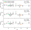 |
Fig. 9 Bottom and middle panels show the distribution of the (α)LOS parameter for the FP and SP as a function of the dynamical age Nh for all clusters in the sample (gray circles). The upper panel shows the distribution of the rotation differences (αSP − αSP)LOS. The dashed lines represent the linear best-fit to the GC distribution. In all panels, the star symbols refer to the results obtained for the stacked analysis on the dynamically young (green) and old (orange) samples. The size of the star matches the amplitude of the errorbars. |
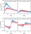 |
Fig. 12 Best-fit results of kinematic analysis of dynamically young (Nh < 8) and old (Nh > 8) stacked samples. FP is in red and SP in blue. The lower panels refer to the LOS rotation, while the upper row shows the results for the TAN velocity component. |
5.2 Ellipticity
In general a rotating system is also expected to be flattened in the direction perpendicular to the rotation axis (Chandrasekhar 1969). Under the assumption that GCs can be described by the same dynamical model, such as an isotropic oblate rotator (e.g., Varri & Bertin 2012), stronger rotation would be expected in more flattened systems. However, various effects can dilute a possible correlation, the most important ones being anisotropies, inclination effects, or tidal forces from the Milky Way (see van den Bergh 2008 for an estimate of the impact of the latter). Nevertheless, Fabricius et al. (2014) and Kamann et al. (2018) were able to reveal a correlation between cluster rotation and ellipticity in a sample of Galactic GCs (see also Lanzoni et al. 2018a; Dalessandro et al. 2021a; Leanza et al. 2023) for similar analysis on specific clusters).
Following on from those results, we searched for any link between MP rotation and ellipticity for all clusters in our sample. The results of such a comparison for population TOT are reported in Appendix C. Interestingly, we find a clear and significant correlation between these two quantities (Spearman rank correlation test gives probabilities of ~99.9%), which is in good agreement with previous results by Fabricius et al. (2014) and Kamann et al. (2018).
Here, we explore in some detail whether the MP rotation patterns are linked to their morphological 2D spatial distributions. We compared the ellipticity estimates obtained as described in Sec. 4 with the (α)LOS MP values in Fig. 13. Both populations show a positive correlation between (α)LOS and ε, with Spearman rank correlation probabilities Pspear ~ 80% and Pspear > 99.9% for the FP and SP, respectively. In detail, the FP shows a pretty flat distribution of (αFP)LOS up to ellipticity values of ε ~ 0.2. Then, (αFP)LOS starts to increase almost linearly with ε. As discussed in Sec. 5.1, the SP tends to show larger values of rotation than the FP. Likely driven by such a stronger rotation, in the upper panel of Fig. 13, we observe that (αSP)LOS follows a nicely linear correlation with ε for the entire range of ellipticity values sampled by the target GCs.
Following the analysis by Fabricius et al. (2014) and Kamann et al. (2018), we computed the differences between the PA values obtained in Sec. 4 for the 2D stellar spatial distribution and the best-fit rotation axis position angles (PA0). Interestingly, while the distribution of the difference is pretty scattered, we find that the average value for the systems in our sample is ~85°, thus implying that the stellar density distribution is on average flattened in the direction perpendicular to the rotation axis. This behavior is in general agreement with what is expected for a rotating system, and it is qualitatively consistent with what was predicted, for example, by the models introduced by Varri & Bertin (2012) and previously found in other observational studies (e.g., Bianchini et al. 2013; Bellini et al. 2017; Lanzoni et al. 2018a; Dalessandro et al. 2021a; Leanza et al. 2022).
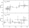 |
Fig. 13 Distributions of (α)LOS parameter for FP and SP (lower and upper panel respectively) as a function of the best-fit ellipticity values (Sec. 4) for the two subpopulations. |
5.3 Dynamical simulations
To conclude the discussion about the rotational properties of MPs in our target GCs, we briefly present the results of a set of N-body simulations aimed at exploring the evolution of rotating MP clusters. A full discussion and detailed description of the results of these simulations will be presented in White et al. (in prep.). Here, we only report the evolutionary path followed by the α parameter introduced in this paper to trace the strength of rotation of FP and SP stars and their difference. In our simulations, we only focused on the long-term dynamics driven by the effects of two-body relaxation for star clusters evolving in the external tidal field of their host galaxy. Each system starts with 105 stars with masses between 0.1 and 1 M⊙ distributed according to a Kroupa (2001) stellar initial mass function. Our systems start with an equal number of FP and SP stars; following the general properties emerging from a few studies of the formation of SP stars in rotating clusters (see, e.g., Bekki 2010, 2011; Lacchin et al. 2022), the SP is initially more centrally concentrated and more rapidly rotating than the FP. The two populations rotate around a common axis. To explore the interplay between internal dynamics and the effects due to the external tidal field, we explored models with different angles δ between the internal rotation axis and the rotation axis of the cluster orbital motion around the center of the host galaxy. In particular, we explored systems with values of δ equal to 0°, 45°, 90°, and 180°. The simulations were run with the NBODY6++GPU code (Wang et al. 2015). In Fig. 14, we show the time5 evolution of αFP, αSP, and (αSP − αFP) for these models using rotational velocity profiles calculated for both the LOS (left panel) and the TAN component (right panel). For these plots we adopt an ideal line of sight perpendicular to the cluster angular momentum or parallel to it. We emphasize that these simulations are not aimed at a detailed comparison with observations, but they serve as a guide to illustrate the extent of the effects of dynamical processes on the initial differences between the rotational kinematics of the FP and SP populations. We also reiterate that our simulations are focussed on the effects of two-body relaxation and do not include early dynamical phases such as those during which a star cluster responds to the mass loss due to stellar evolution, which can have an effect on the subpopulations’ dynamical differences (see, e.g., Vesperini et al. 2021; Sollima 2021).
By construction, the α values derived for the SP are significantly larger -by about a factor of 2–3- than those of the FP. The results of our simulations show that the effects of two-body relaxation lead to a rapid and significant reduction of the initial difference between the FP and the SP rotation in the first 2–3 half-mass relaxation times reaching values of (αSP − αFP) similar to those found in our observational analysis. Then, at later dynamical ages, (αSP − αFP) keeps decreasing at a slower pace, and it progressively approaches values close to zero around ten relaxation times, at which point FP and SP stars rotate at the same velocity. We note that, as already discussed in Sec. 5.1 and in agreement with what was found in the observations, the rotation strength for both the FP and SP along with their difference is stronger when a PM-like projection is considered (Fig. 14). The behavior described by the simulations is generally in good agreement with the observed trends (Figs. 9–11). Such an agreement strongly suggests that both the rotational differences and the mild trend between the rotation strength and the dynamical age revealed by our observational analysis are consistent with those expected for the long-term dynamical evolution of GCs born with an SP initially rotating more rapidly than the FP.
6 Results: anisotropy
6.1 Observations
We investigated the differences in the mean anisotropy properties of MPs by defining the following parameter:
![Mathematical equation: $\[\alpha_\beta=\int_0^1\left(\beta\left(R_l\right)_X\right) \mathrm{d} R_l;\]$](/articles/aa/full_html/2024/11/aa51054-24/aa51054-24-eq120.png) (11)
(11)
here, Rl represents the distance from the cluster center normalized to the value of the cluster’s Jacobi radius (from Baumgardt et al. 2019) to allow a meaningful comparison among different systems (see Table 2). From a geometrical point of view, Eq. (11) represents the area subtended by the best-fit, radially normalized anisotropy profile (as defined in Sect. 3.2). By definition, if a subpopulation is radially anisotropic, αβ will have positive values, while it will attain negative values in the case of tangential anisotropy. Differences between the anisotropy properties of MPs are given by ![Mathematical equation: $\[\left(\alpha_\beta^{S P}-\alpha_\beta^{F P}\right)\]$](/articles/aa/full_html/2024/11/aa51054-24/aa51054-24-eq121.png) . As before, errors on αβ were obtained by propagating the posterior probability distributions obtained from the MCMC analysis for the best-fit anisotropy profiles.
. As before, errors on αβ were obtained by propagating the posterior probability distributions obtained from the MCMC analysis for the best-fit anisotropy profiles.
Similarly to the rotation analysis, Fig. 15 shows the variation of αβ as a function of the dynamical age for the FP and SP in the bottom and middle panel, while the distribution of ![Mathematical equation: $\[\left(\alpha_\beta^{S P}-\alpha_\beta^{F P}\right)\]$](/articles/aa/full_html/2024/11/aa51054-24/aa51054-24-eq122.png) is shown in the top panel.
is shown in the top panel. ![Mathematical equation: $\[\alpha_\beta^{F P}\]$](/articles/aa/full_html/2024/11/aa51054-24/aa51054-24-eq123.png) shows a flat distribution around ~0 at any Nh, thus suggesting that the FP is on average isotropic for all GCs in the sample, independently on their dynamical ages. On the contrary, the
shows a flat distribution around ~0 at any Nh, thus suggesting that the FP is on average isotropic for all GCs in the sample, independently on their dynamical ages. On the contrary, the ![Mathematical equation: $\[\alpha_\beta^{S P}\]$](/articles/aa/full_html/2024/11/aa51054-24/aa51054-24-eq124.png) shows a non-negligible variation as a function of time. In fact, for dynamically young clusters,
shows a non-negligible variation as a function of time. In fact, for dynamically young clusters, ![Mathematical equation: $\[\alpha_\beta^{S P}\]$](/articles/aa/full_html/2024/11/aa51054-24/aa51054-24-eq125.png) is positive (i.e., SP is radially anisotropic) and it becomes isotropic only for the dynamically older systems. To better highlight such a trend, we can use the two GC subgroups defined in Sect. 5.1. At a face value, GCs with Nh < 8 (dynamically young) have a mean
is positive (i.e., SP is radially anisotropic) and it becomes isotropic only for the dynamically older systems. To better highlight such a trend, we can use the two GC subgroups defined in Sect. 5.1. At a face value, GCs with Nh < 8 (dynamically young) have a mean ![Mathematical equation: $\[\alpha_\beta^{S P}\]$](/articles/aa/full_html/2024/11/aa51054-24/aa51054-24-eq126.png) value of 0.40 ± 0.20, while for dynamically older clusters the mean value is −0.09 ± 0.23 (dashed lines in Fig. 15). Such a difference is very nicely described by the comparison between the best-fit results obtained for MPs in the two stacked samples as shown in Fig. 16. Indeed, when the anisotropy analysis is performed on the two stacked subsamples, we find that
value of 0.40 ± 0.20, while for dynamically older clusters the mean value is −0.09 ± 0.23 (dashed lines in Fig. 15). Such a difference is very nicely described by the comparison between the best-fit results obtained for MPs in the two stacked samples as shown in Fig. 16. Indeed, when the anisotropy analysis is performed on the two stacked subsamples, we find that ![Mathematical equation: $\[\alpha_\beta^{S P}\]$](/articles/aa/full_html/2024/11/aa51054-24/aa51054-24-eq127.png) = 0.23 ± 0.03 at dynamically young ages, while for dynamically older clusters we obtain
= 0.23 ± 0.03 at dynamically young ages, while for dynamically older clusters we obtain ![Mathematical equation: $\[\alpha_\beta^{S P}\]$](/articles/aa/full_html/2024/11/aa51054-24/aa51054-24-eq128.png) = 0.04 ± 0.03, thus implying that the difference in the average SP orbital anisotropy is significant at a ~5σ level. For comparison, we computed the same quantities for the FP on the stacked clusters. As expected, in this case mean values are virtually indistinguishable within the errors. The different behavior between the average orbital properties of FP and SP stars is further highlighted by the distribution of
= 0.04 ± 0.03, thus implying that the difference in the average SP orbital anisotropy is significant at a ~5σ level. For comparison, we computed the same quantities for the FP on the stacked clusters. As expected, in this case mean values are virtually indistinguishable within the errors. The different behavior between the average orbital properties of FP and SP stars is further highlighted by the distribution of ![Mathematical equation: $\[\left(\alpha_\beta^{S P}-\alpha_\beta^{F P}\right)\]$](/articles/aa/full_html/2024/11/aa51054-24/aa51054-24-eq129.png) . In dynamically young GCs, SP is systematically more radially anisotropic than the FP (mean difference being 0.44 ± 0.31), then they both become compatible with being isotropic at later dynamical stages (−0.08 ± 0.37). The analysis of the two stacked subsamples provides values of
. In dynamically young GCs, SP is systematically more radially anisotropic than the FP (mean difference being 0.44 ± 0.31), then they both become compatible with being isotropic at later dynamical stages (−0.08 ± 0.37). The analysis of the two stacked subsamples provides values of ![Mathematical equation: $\[\left(\alpha_\beta^{S P}-\alpha_\beta^{F P}\right)\]$](/articles/aa/full_html/2024/11/aa51054-24/aa51054-24-eq130.png) = 0.28 ± 0.07 and 0.09 ± 0.07 for the dynamically young and old groups, respectively, thus implying that there is a real orbital velocity distribution difference between FP and SP stars with a significance of ~3.5σ.
= 0.28 ± 0.07 and 0.09 ± 0.07 for the dynamically young and old groups, respectively, thus implying that there is a real orbital velocity distribution difference between FP and SP stars with a significance of ~3.5σ.
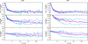 |
Fig. 14 Time evolution of rotational parameters αFP, αSP, and their differences (see Sect. 5.1) for the simulations described in Sect. 5.3. The blue line corresponds to the model with δ = 0°; the pink, cyan, and purple correspond to δ = 45°, 90°, and 180°, respectively. |
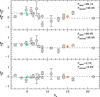 |
Fig. 15 Bottom and middle panels show the distribution of the anisotropy parameter αβ for the FP and SP subpopulations of GCs in the sample (gray circles) as a function of Nh. The top panel shows the differential trend |
![Mathematical equation: $\[\alpha_\beta^{\mathrm{SP}}-\alpha_\beta^{\mathrm{FP}}\]$](/articles/aa/full_html/2024/11/aa51054-24/aa51054-24-eq131.png)
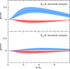 |
Fig. 16 Best-fit results of anisotropy analysis of MPs in the two stacked samples. The upper panel shows the best-fit anisotropy profiles of the FP (red) and SP (blue) subpopulations as obtained for the stacked sample of dynamically young GCs, while the lower panel refers to dynamically old systems. |
6.2 Dynamical models
The difference between the anisotropy of the FP and SP populations is consistent with the predictions of a number of theoretical investigations of the dynamics of MP clusters. These studies find that in clusters where the SP forms more centrally concentrated than the FP, the SP is generally characterized by a more radially anisotropic velocity distribution than the FP (see, e.g., Bellini et al. 2015; Hénault-Brunet et al. 2015; Tiongco et al. 2019; Vesperini et al. 2021; Sollima 2021). In order to illustrate the expected strength and evolution of the differences between the anisotropy of the FP and SP populations, as measured by the parameter ![Mathematical equation: $\[\left(\alpha_\beta^{S P}-\alpha_\beta^{F P}\right)\]$](/articles/aa/full_html/2024/11/aa51054-24/aa51054-24-eq132.png) introduced in this paper, in Fig. 17 we show the time evolution of
introduced in this paper, in Fig. 17 we show the time evolution of ![Mathematical equation: $\[\alpha_\beta^{F P}, \alpha_\beta^{S P}\]$](/articles/aa/full_html/2024/11/aa51054-24/aa51054-24-eq133.png) , and
, and ![Mathematical equation: $\[\left(\alpha_\beta^{S P}-\alpha_\beta^{F P}\right)\]$](/articles/aa/full_html/2024/11/aa51054-24/aa51054-24-eq134.png) for three Monte Carlo simulations following the dynamical evolution of MP clusters with different initial conditions. The Monte Carlo simulations were run with the MOCCA code (Hypki & Giersz 2013; Giersz et al. 2013; see also Vesperini et al. 2021; Hypki et al. 2022 for the specific case of GCs with MPs). A full presentation of the kinematics and phase-space properties of these systems will be presented in a separate paper (Aros et al. in prep.). The three models for which we present the anisotropy evolution in Fig. 17 all start with a ratio of the SP to total mass equal to 0.2. The total number of stars is equal to N = 106 (hereafter, we use the ID N1M for these models) or 0.5 × 10⁶ (with ID N05M), and stars have been extracted from a Kroupa (2001) initial stellar mass function between 0.1 and 100 M⊙. The SP is initially more concentrated than the FP; for two models, the initial ratio for the FP-to-SP half-mass radii is equal to 20 (N1Mr20 and N05Mr20), and it is equal to ten for one model (N1Mr10). Both populations are initially characterized by a non-rotating, isotropic velocity distribution. All models include the effects of mass loss due to stellar evolution, two-body relaxation, binary interactions, and a tidal truncation (see Vesperini et al. 2021 for further details on the evolutionary processes included in these simulations). As shown in Fig. 17, in all models the SP is characterized by a more radially anisotropic velocity distribution than the FP. Even if both populations are initially isotropic, the development of a stronger radial anisotropy for the SP is the consequence of its initial more centrally concentrated spatial distribution (see, e.g., Tiongco et al. 2019; Vesperini et al. 2021). The differences in anisotropy between the two populations gradually decrease as the systems evolve. As shown by the results of our simulations, the extent of the differences between the FP and SP anisotropy depends on the initial relative concentration of the two populations being smaller for the model where the initial ratio of the FP to SP half-mass radii is equal to ten (N1MR10) than that for models where this ratio is initially equal to 20 (N1MR20). While we also point out that these simulations have not been specifically designed to provide a detailed fit to observations, but rather to provide guidance in the general interpretation of the observational results, it is interesting to note that the extent of the difference between the anisotropy of the FP and the SP populations as measured by the
for three Monte Carlo simulations following the dynamical evolution of MP clusters with different initial conditions. The Monte Carlo simulations were run with the MOCCA code (Hypki & Giersz 2013; Giersz et al. 2013; see also Vesperini et al. 2021; Hypki et al. 2022 for the specific case of GCs with MPs). A full presentation of the kinematics and phase-space properties of these systems will be presented in a separate paper (Aros et al. in prep.). The three models for which we present the anisotropy evolution in Fig. 17 all start with a ratio of the SP to total mass equal to 0.2. The total number of stars is equal to N = 106 (hereafter, we use the ID N1M for these models) or 0.5 × 10⁶ (with ID N05M), and stars have been extracted from a Kroupa (2001) initial stellar mass function between 0.1 and 100 M⊙. The SP is initially more concentrated than the FP; for two models, the initial ratio for the FP-to-SP half-mass radii is equal to 20 (N1Mr20 and N05Mr20), and it is equal to ten for one model (N1Mr10). Both populations are initially characterized by a non-rotating, isotropic velocity distribution. All models include the effects of mass loss due to stellar evolution, two-body relaxation, binary interactions, and a tidal truncation (see Vesperini et al. 2021 for further details on the evolutionary processes included in these simulations). As shown in Fig. 17, in all models the SP is characterized by a more radially anisotropic velocity distribution than the FP. Even if both populations are initially isotropic, the development of a stronger radial anisotropy for the SP is the consequence of its initial more centrally concentrated spatial distribution (see, e.g., Tiongco et al. 2019; Vesperini et al. 2021). The differences in anisotropy between the two populations gradually decrease as the systems evolve. As shown by the results of our simulations, the extent of the differences between the FP and SP anisotropy depends on the initial relative concentration of the two populations being smaller for the model where the initial ratio of the FP to SP half-mass radii is equal to ten (N1MR10) than that for models where this ratio is initially equal to 20 (N1MR20). While we also point out that these simulations have not been specifically designed to provide a detailed fit to observations, but rather to provide guidance in the general interpretation of the observational results, it is interesting to note that the extent of the difference between the anisotropy of the FP and the SP populations as measured by the ![Mathematical equation: $\[\left(\alpha_\beta^{S P}-\alpha_\beta^{F P}\right)\]$](/articles/aa/full_html/2024/11/aa51054-24/aa51054-24-eq135.png) and its time evolution is generally consistent with the findings of our observational analysis (Fig. 15). The general agreement between observations and simulations lends further support to the interpretation of the observed difference between the FP and SP anisotropy and its variation with the clusters’ dynamical ages as the manifestation of the different dynamical paths followed by subsystems with different initial spatial distributions.
and its time evolution is generally consistent with the findings of our observational analysis (Fig. 15). The general agreement between observations and simulations lends further support to the interpretation of the observed difference between the FP and SP anisotropy and its variation with the clusters’ dynamical ages as the manifestation of the different dynamical paths followed by subsystems with different initial spatial distributions.
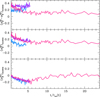 |
Fig. 17 Time evolution of anisotropy parameters defined in Sec. 6.1 for the FP (bottom panel), the SP (middle panel), and their difference (top panel) in the three Monte Carlo simulations described in Sec. 6.2 (N1Mr10 blue line, N1M purple line; N05M pink line). Time is normalized by the half-mass relaxation time. |
7 Comparison with the literature
In Appendix C, we report on a quantitative comparison between the results obtained in the present work and those available in the literature for the TOT population in each cluster. Here, we detail the comparison with previous works focusing on the kinematics of MPs. We stress that the full 3D kinematic analysis presented in this paper is the first ever obtained for MPs. Hence, in the following our comparison is limited to studies considering a single velocity component.
Our sample has six GCs in common with the recent analysis by Martens et al. (2023) based on MUSE LOS velocities. The authors were able to find MP best-fit solutions for both the velocity dispersion and rotation profiles for three of them (namely 47 Tuc, NGC 5904, and NGC 6093), while for NGC 3201 and NGC 6254 they report only conservative upper limits for the MP rotation amplitudes, and for NGC 1904 they provide information only for the TOT population. Figure 18 shows the distributions of the differences in terms of σ0 (which is defined as σmax in Martens et al. 2023), Arot (υmax in Martens et al. 2023), and Rpeak for the FP and SP subpopulations. A good agreement is observed both for the MP central velocity dispersion values (left panel of Fig. 18) and the rotation amplitude (middle panel), with the most discrepant value being that corresponding to the rotation of the SP in 47 Tuc. Within the errors, there is also a reasonable match between the values of Rpeak. We note, however, that while the sample is certainly small, the estimates of Rpeak by Martens et al. (2023) tend to be slightly smaller than those derived in this work. This might be somehow linked to the smaller radial coverage of the Martens et al. (2023) analysis. In fact, all values derived by Martens et al. (2023) for the clusters in common are located well outside the MUSE field of view, and therefore they might be only partially constrained by their analysis.
The sample analyzed in this work also counts four GCs in common with Cordoni et al. (2020), namely 47 Tuc, NGC 288, NGC 5904, and NGC 6254. Our results are in agreement with theirs in that 47 Tuc and NGC 5904 are the systems showing the larger rotation among the clusters in common. However, at odds with their results, we also find that in both GCs the SP show a larger rotation (as inferred both by Arot and α values) than the FP. Also, within the uncertainties, we do not find evidence of any significant misalignment of the FP and SP rotation curves for these systems, nor in terms of position angles and inclination, as constrained by both the LOS and the full 3D analysis. Finally, our analysis is in good agreement with the results presented by Cordero et al. (2017) for the MP rotation patterns of M 13.
As for the anisotropy, the results obtained in this work are in qualitative agreement with those found for GCs M 13, NGC 2808, and 47 Tuc by Richer et al. (2013), Bellini et al. (2015) and Milone et al. (2018). More generally, they are in good qualitative agreement with those recently obtained in the innermost regions (R< 100″) for a sample of Galactic GCs by Libralato et al. (2023) using HST PMs to search for average differences between the anisotropy profiles of MPs.
8 Summary and conclusions
We present the first self-consistent 3D kinematic analysis of MPs for a sample of Galactic GCs. The study targets 16 systems spanning a broad range of dynamical ages (2 < Nh < 25) and is based on a large and mostly homogeneous observational dataset securing several hundreds of accurate LOS velocities and PMs for each cluster and sampling virtually their entire extension.
Our study is mainly focused on the analysis of the MP rotation along the three velocity components and the anisotropy of their velocity distributions. The adopted approach is aimed at providing new insights into the long-term evolution of the kinematic properties of MPs (and their differences) for the entire sample of GCs and for the entire dynamical age covered by our analysis instead of focusing on the kinematic differences in specific clusters. To this aim, starting from the observed velocity distributions we defined a few key quantities to quantitatively and homogeneously compare the results obtained for all the observed GCs.
Our analysis provides the first observational determination of the dynamical path followed by MP kinematic properties during their long-term evolution. The main observational results we find can be schematically summarized as follows.
We observe evidence of differential rotation between MPs with the SP preferentially rotating more rapidly than the FP. This result is consistent (although with different amplitudes) along both the LOS and TAN velocity components, as well as in the full 3D analysis. In all GCs in our sample, we find that the rotation position and inclination angles are consistent within the uncertainties between FP and SP.
The strength of the rotation signal of both FP and SP subpopulations nicely correlate with the ellipticity values derived for the two subpopulations. In addition, we find that the rotation axis position angle is typically perpendicular to the ellipses’ major axis.
The difference in the rotation strength between MPs is mildly anticorrelated with the cluster dynamical age. In particular, differences are larger for dynamically young clusters, and they become progressively indistinguishable as dynamical evolution proceeds.
Stars belonging to different subpopulations show different average velocity distribution properties. FPs are characterized by isotropic velocity distributions at any dynamical age probed by our sample. On the contrary, the SP of dynamically young GCs have a radially anisotropic velocity distribution that becomes isotropic in more advanced evolutionary stages.
The combination of these results with the analysis of the MP radial distributions of a representative sample of GCs carried out in our previous paper (Dalessandro et al. 2019), provides a full picture of the present-day kinematic and structural properties of MPs in GCs and of their evolution. The comparison with dynamical models following the long-term evolution of MPs in GCs suggests that these properties, and their evolution with dynamical age, are generally in good agreement with those expected in clusters forming with an SP subsystem that is initially more centrally concentrated and more rapidly rotating than the FP (see e.g., D’Ercole et al. 2008; Bekki 2010; Calura et al. 2019; Lacchin et al. 2022). In turn, this could suggest (see, e.g., Hénault-Brunet et al. 2015 and discussion in Martens et al. 2023) that GCs experienced multiple events of star formation during their early phases of evolution, with the rotation properties being the more stringent discriminating factors. In fact, according to multi-epoch formation models, the SP is expected to form a low-mass, more centrally concentrated and more rapidly rotating stellar subsystem than the FP. In such a configuration, dissipative accretion processes of material ejected by FP stars and angular momentum conservation in subsystems with different initial concentrations can produce a larger initial rotation of the SP subsystem (Bekki 2011; Hénault-Brunet et al. 2015; Tiongco et al. 2017). Interestingly, it has been shown (e.g., Bekki 2011) that even if only a very small fraction of the kinetic energy of the FP is in the form of bulk rotation energy, SP stars can acquire a much stronger rotation than what remains in the FP.
It is important to note that, as shown in this paper and in a number of previous studies, early and long-term evolution can significantly reduce the initial differences between the FP and SP rotational velocities making them virtually indistinguishable in dynamical old systems. The combination of these physical effects with the observational uncertainties arising from the limited available stellar samples, partial cluster coverage and possible biases introduced by the different rotation inclination angles, can make it extremely difficult to capture present-day kinematic differences between MPs, in particular in the LOS velocity component. As a consequence, it is important to use some caution in drawing conclusions about the physical mechanisms at the basis of GC formation and early evolution based on the present-day kinematic and structural properties of individual systems or small samples.
A homogeneous combination of data obtained with multi-object spectrographs and Gaia (as presented in this paper), which are particularly sensitive to the intermediate and large cluster-centric distances in GCs, with Integral Field Unit LOS RVs and HST absolute PMs sampling more efficiently the clusters’ innermost regions (see, e.g., Martens et al. 2023; Libralato et al. 2023), along with an increase of the cluster sample size, represents a natural and promising next step that could potentially enable the exploration of additional physical ingredients at play. The results of this study clearly demonstrate that significant advances in our understanding of cluster formation and early evolution are only possible through a multifaceted and multi-diagnostic approach and by combining state-of-the-art observations and simulations.
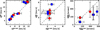 |
Fig. 18 Comparison between best-fit σ0, Arot, and Rpeak values obtained for MPs in the present work and by Martens et al. (2023). Blue dots refer to SP and red ones to FP results. |
Acknowledgements
The authors thank the anonymous referee for the careful reading of the paper and the useful comments that improved the presentation of this work. E.D. acknowledges financial support from the Fulbright Visiting Scholar program 2023. E.D. and A.D.C. are also grateful for the warm hospitality of the Indiana University where part of this work was performed. E.D. and M.C. acknowledge financial support from the project Light-on-Dark granted by MIUR through PRIN2017-2017K7REXT. E.V. acknowledges support from NSF grant AST-2009193. E.V. acknowledges also support from the John and A-Lan Reynolds Faculty Research Fund. The research activities described in this paper have been co-funded by the European Union - NextGenerationEU within PRIN 2022 project n.20229YBSAN - Globular clusters in cosmological simulations and in lensed fields: from their birth to the present epoch.
Appendix A Additional table
Best-fit values of the main MP kinematic properties.
Appendix B Incompleteness effects
We constrained the possible impact of the kinematic samples’ size and of their (radially dependent) incompleteness (mainly caused by the intrinsically limited allocation efficiency of multi-object spectrographs) on the results obtained in this work by using the dynamical simulations described in Sects. 5 and 6.
In detail, we estimated the completeness (C) of the observed kinematic samples and its radial variation as the ratio between the number of RGB stars detected in the photometric catalogs and those with LOS RVs and/or PMs measures within concentric radial annuli at different cluster-centric distances. While we acknowledge that these estimates represent a lower-limit to the real incompleteness, as photometric catalogs are not fully complete, we note that our targets are RGB stars, which are among the brightest stars in GC CMDs and therefore they are only moderately affected by incompleteness even when ground-based catalogs are adopted.
We then extracted randomly from the simulations sub-samples of stars with similar sizes as the observed ones for a large number of times. We applied the derived completeness curves to these sub-samples to make them as similar as possible to the observed catalogs. Finally we run the same kinematic analysis described in Sect. 3. We find that, while the limited sample sizes and incompleteness have an impact on the overall noise of the observed kinematic profiles and, as a consequence, on the uncertainties associated to the derived parameters, they do not have a significant impact on the final results.
Appendix C Global kinematics and comparison with the literature
Figure C.1 shows the distribution of the α values derived for the entire population along both the LOS and TAN velocity components, and of the ![Mathematical equation: $\[\omega_{3 D}^{\mathrm{TOT}}\]$](/articles/aa/full_html/2024/11/aa51054-24/aa51054-24-eq560.png) , as a function of Nh. As expected, both αTOT (for both LOS and TAN) and the
, as a function of Nh. As expected, both αTOT (for both LOS and TAN) and the ![Mathematical equation: $\[\omega_{3 D}^{\mathrm{TOT}}\]$](/articles/aa/full_html/2024/11/aa51054-24/aa51054-24-eq561.png) distributions show pretty clear anti-correlations with Nh. In fact, while dynamically young GCs attain larger values of rotation parameters, with the only significant exception being M 3, the rotation strength progressively decreases as dynamical evolution proceeds. By performing a Spearman rank correlation test we find that such anti-correlations have a significance of ~ 98% for the LOS and > 99.9% for both the TAN and the 3D analysis, with the 3D case being the most significant. In general, these results are in very good agreement with previous analysis (e.g., Kamann et al. 2018; Sollima et al. 2019) and they further strengthen the conclusion that the present-day cluster rotation is the relic of that imprinted at the epoch of cluster formation, which has been then progressively dissipated via two-body relaxation.
distributions show pretty clear anti-correlations with Nh. In fact, while dynamically young GCs attain larger values of rotation parameters, with the only significant exception being M 3, the rotation strength progressively decreases as dynamical evolution proceeds. By performing a Spearman rank correlation test we find that such anti-correlations have a significance of ~ 98% for the LOS and > 99.9% for both the TAN and the 3D analysis, with the 3D case being the most significant. In general, these results are in very good agreement with previous analysis (e.g., Kamann et al. 2018; Sollima et al. 2019) and they further strengthen the conclusion that the present-day cluster rotation is the relic of that imprinted at the epoch of cluster formation, which has been then progressively dissipated via two-body relaxation.
Figure C.2 shows the distribution of ![Mathematical equation: $\[\alpha_{\mathrm{LOS}}^{\mathrm{TOT}}\]$](/articles/aa/full_html/2024/11/aa51054-24/aa51054-24-eq562.png) with the cluster ellipticity obtained as described in Sect. 3. As expected (see discussion and references in Sect. 5.2), a nice correlation between rotation and ellipticity is observed also for the total population in very good agreement with previous findings by Fabricius et al. (2014) and Kamann et al. (2018).
with the cluster ellipticity obtained as described in Sect. 3. As expected (see discussion and references in Sect. 5.2), a nice correlation between rotation and ellipticity is observed also for the total population in very good agreement with previous findings by Fabricius et al. (2014) and Kamann et al. (2018).
While the focus of this work is on the MP kinematics, nevertheless it is useful to compare the results obtained for the TOT population with those largely available in the literature to have an indication about the general performance of the adopted approach and data-sets. Detailed one-to-one comparisons with recent results obtained in the literature (Bellazzini et al. 2012; Ferraro et al. 2018; Lanzoni et al. 2018a,b; Baumgardt et al. 2019; Sollima et al. 2019) for the TOT population are shown in Figs. C.3 and C.4. In general, a quite good agreement is observed with all the compilations considered here.
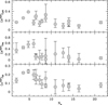 |
Fig. C.1 Distribution of the three rotation parameters defined in this work for the LOS, PM and 3D velocity components, as a function of the dynamical age (Nh) for the total population (TOT) of GCs in our sample. |
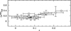 |
Fig. C.2 Distribution of the (αTOT)LOS parameter for the total population as a function of the best-fit ellipticity values derived as described in Sect. 4. |
Our sample has 6 GCs in common with Bellazzini et al. (2012). A nice match is observed both in terms of α0 and Arot (top row of Fig. C.3) with the only exception being NGC 6171 for which Bellazzini et al. (2012) finds a rotation amplitude 4–5 times larger than the one obtained in this work. Given the estimate by Bellazzini et al. (2012), NGC 6171 would be a very fast rotator, with Arot/σ0 ~ 0.7. However, it is important to note, that the sample of LOS RVs used by Bellazzini et al. (2012) for this cluster includes only 31 stars in total, resulting the smallest sample of LOS RVs in their analysis. Here we sample the kinematic profile of NGC 6171 with 184 LOS RVs (see Table 1). We note also that NGC 6171 results to have a significantly smaller rotation amplitude (1.2 km/s) than what found by Bellazzini et al. (2012) in the analysis by Ferraro et al. (2018) and it is classified as non rotator by Sollima et al. (2019)
As for the comparison with results by Ferraro et al. (2018), we stress that while the spectroscopic sample is largely similar, the adopted kinematic analysis (both the discrete and con tinuous ones) is significantly different for the rotation study in particular (see Ferraro et al. 2018 for details). Hence, it is not surprising that while the derived central velocity dispersion values are in excellent agreement for the entire sample (middle row of Fig. C.3), the distribution of differences for Arot is more scattered, while still showing a reasonable match within the errors. In this case, the most significant discrepancy is observed for NGC 5927, for which Ferraro et al. (2018) derived Arot = 2.3 km/s, while we find ![Mathematical equation: $\[A_{rot}=0.76_{-0.54}^{+0.90}\]$](/articles/aa/full_html/2024/11/aa51054-24/aa51054-24-eq563.png) km/s. For this cluster also Sollima et al. (2019) derived a low probability of rotation.
km/s. For this cluster also Sollima et al. (2019) derived a low probability of rotation.
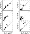 |
Fig. C.3 Comparison between the best-fit σ0 and Arot values obtained for the TOT sample for the clusters in common between the present work and Bellazzini et al. (2012) – B12, Ferraro et al. (2018) – F18 and Petralia et al. (2024) – P24. |
In the bottom row of Fig. C.3 we compare the results of this work with those recently obtained by Petralia et al. (2024) by using APOGEE spectra for a sample of Galactic GCs. For Arot we use the semi-amplitude of the Afit values reported in their work. A reasonable overall agreement is observed also in this case for the clusters in common, however 47 Tuc and NGC 5904 result to have larger central velocity dispersion values and peak of rotation than in our work.
Finally, as shown in Fig. C.4 (left panel) a reasonably good match is also found with the σ0 estimates by Baumgardt et al. (2019). Among the clusters in common with Sollima et al. (2019), the only significantly discrepant result is that of 47 Tuc, which results to have a ~ 25% larger rotation in this work. However, we note that in this case, as for the entire sample, both the i and θ0 values are in very good agreement. In this respect, it is also interesting to highlight the nice match in terms of both the observed rotation amplitude and angles of the 3D rotation of 47 Tuc obtained in this work and those inferred by means of a detailed comparison between HST PMs and theoretical models of rotating clusters by Bellini et al. (2017).
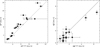 |
Fig. C.4 Left panel: Comparison with the best-fit σ0 values obtained by Baumgardt et al. (2019) − B19 – for the total population of GCs in common with the present work. Right panel: One-to-one comparison of the 3D rotation amplitude values A3D found by Sollima et al. (2019) – S19 – and the present analysis. |
References
- Aarseth, S. J. 2003, Gravitational N-Body Simulations, ed. S. J. Aarseth (Cambridge, UK: Cambridge University Press), 430 [Google Scholar]
- Bastian, N., & Lardo, C. 2015, MNRAS, 453, 357 [NASA ADS] [CrossRef] [Google Scholar]
- Bastian, N., & Lardo, C. 2018, ARA&A, 56, 83 [Google Scholar]
- Bastian, N., Lamers, H. J. G. L. M., de Mink, S. E., et al. 2013, MNRAS, 436, 2398 [CrossRef] [Google Scholar]
- Baumgardt, H., Hilker, M., Sollima, A., et al. 2019, MNRAS, 482, 5138 [NASA ADS] [CrossRef] [Google Scholar]
- Bekki, K. 2010, ApJ, 724, L99 [CrossRef] [Google Scholar]
- Bekki, K. 2011, MNRAS, 412, 2241 [NASA ADS] [CrossRef] [Google Scholar]
- Bellazzini, M., Bragaglia, A., Carretta, E., et al. 2012, A&A, 538, A18 [NASA ADS] [CrossRef] [EDP Sciences] [Google Scholar]
- Bellini, A., Vesperini, E., Piotto, G., et al. 2015, ApJ, 810, L13 [NASA ADS] [CrossRef] [Google Scholar]
- Bellini, A., Milone, A. P., Anderson, J., et al. 2017, ApJ, 844, 164 [NASA ADS] [CrossRef] [Google Scholar]
- Bianchini, P., Varri, A. L., Bertin, G., et al. 2013, ApJ, 772, 67 [NASA ADS] [CrossRef] [Google Scholar]
- Bianchini, P., van der Marel, R. P., del Pino, A., et al. 2018, MNRAS, 481, 2125 [Google Scholar]
- Bragaglia, A., Carretta, E., D’Orazi, V., et al. 2017, A&A, 607, A44 [NASA ADS] [CrossRef] [EDP Sciences] [Google Scholar]
- Cadelano, M., Saracino, S., Dalessandro, E., et al. 2020, ApJ, 895, 54 [NASA ADS] [CrossRef] [Google Scholar]
- Cadelano, M., Dalessandro, E., Salaris, M., et al. 2022, ApJ, 924, L2 [NASA ADS] [CrossRef] [Google Scholar]
- Cadelano, M., Pallanca, C., Dalessandro, E., et al. 2023, A&A, 679, L13 [NASA ADS] [CrossRef] [EDP Sciences] [Google Scholar]
- Cadelano, M., Dalessandro, E., & Vesperini, E. 2024, A&A, 685, A158 [NASA ADS] [CrossRef] [EDP Sciences] [Google Scholar]
- Carretta, E., Bragaglia, A., Gratton, R., et al. 2009, A&A, 505, 139 [NASA ADS] [CrossRef] [EDP Sciences] [Google Scholar]
- Calura, F., D’Ercole, A., Vesperini, E., Vanzella, E., & Sollima, A. 2019, MNRAS, 489, 3269 [Google Scholar]
- Chandrasekhar, S. 1969, ApJ, 157, 1419 [NASA ADS] [CrossRef] [Google Scholar]
- Chung, C., Yoon, S.-J., & Lee, Y.-W. 2011, ApJ, 740, L45 [NASA ADS] [CrossRef] [Google Scholar]
- Curran, P. A. 2015, Astrophysics Source Code Library [ascl:1504.008] [Google Scholar]
- Cordero, M. J., Hénault-Brunet, V., Pilachowski, C. A., et al. 2017, MNRAS, 465, 3515 [NASA ADS] [CrossRef] [Google Scholar]
- Cordoni, G., Milone, A. P., Mastrobuono-Battisti, A., et al. 2020, ApJ, 889, 18 [Google Scholar]
- D’Antona, F., Vesperini, E., D’Ercole, A., et al. 2016, MNRAS, 458, 2122 [Google Scholar]
- Dalessandro, E., Salaris, M., Ferraro, F. R., et al. 2011, MNRAS, 410, 694 [NASA ADS] [CrossRef] [Google Scholar]
- Dalessandro, E., Schiavon, R. P., Rood, R. T., et al. 2012, AJ, 144, 126 [NASA ADS] [CrossRef] [Google Scholar]
- Dalessandro, E., Ferraro, F. R., Massari, D., et al. 2013, ApJ, 778, 135 [NASA ADS] [CrossRef] [Google Scholar]
- Dalessandro, E., Massari, D., Bellazzini, M., et al. 2014, ApJ, 791, L4 [NASA ADS] [CrossRef] [Google Scholar]
- Dalessandro, E., Lapenna, E., Mucciarelli, A., et al. 2016, ApJ, 829, 77 [NASA ADS] [CrossRef] [Google Scholar]
- Dalessandro, E., Cadelano, M., Vesperini, E., et al. 2018a, ApJ, 859, 15 [NASA ADS] [CrossRef] [Google Scholar]
- Dalessandro, E., Mucciarelli, A., Bellazzini, M., et al. 2018b, ApJ, 864, 33 [NASA ADS] [CrossRef] [Google Scholar]
- Dalessandro, E., Lardo, C., Cadelano, M., et al. 2018c, A&A, 618, A131 [NASA ADS] [CrossRef] [EDP Sciences] [Google Scholar]
- Dalessandro, E., Cadelano, M., Vesperini, E., et al. 2019, ApJ, 884, L24 [Google Scholar]
- Dalessandro, E., Raso, S., Kamann, S., et al. 2021a, MNRAS, 506, 813 [CrossRef] [Google Scholar]
- Dalessandro, E., Varri, A. L., Tiongco, M., et al. 2021b, ApJ, 909, 90 [NASA ADS] [CrossRef] [Google Scholar]
- Decressin, T., Meynet, G., Charbonnel, C., Prantzos, N., & Ekström, S. 2007, A&A, 464, 1029 [NASA ADS] [CrossRef] [EDP Sciences] [Google Scholar]
- Della Croce, A., Dalessandro, E., Livernois, A., et al. 2023, A&A, 674, A93 [NASA ADS] [CrossRef] [EDP Sciences] [Google Scholar]
- de Mink, S. E., Pols, O. R., Langer, N., et al. 2009, A&A, 507, L1 [NASA ADS] [CrossRef] [EDP Sciences] [Google Scholar]
- D’Ercole, A., Vesperini, E., D’Antona, F., McMillan, S. L. W., & Recchi, S. 2008, MNRAS, 391, 825 [CrossRef] [Google Scholar]
- Dotter, A., Sarajedini, A., Anderson, J., et al. 2010, ApJ, 708, 698 [Google Scholar]
- Einsel, C., & Spurzem, R. 1999, MNRAS, 302, 81 [NASA ADS] [CrossRef] [Google Scholar]
- Fabricius, M. H., Noyola, E., Rukdee, S., et al. 2014, ApJ, 787, L26 [NASA ADS] [CrossRef] [Google Scholar]
- Ferraro, F. R., Mucciarelli, A., Lanzoni, B., et al. 2018b, ApJ, 860, 50 [NASA ADS] [CrossRef] [Google Scholar]
- Foreman-Mackey, D., Hogg, D. W., Lang, D., Goodman, J. 2013, PASP, 125, 306 [NASA ADS] [CrossRef] [Google Scholar]
- Gaia Collaboration (Vallenari, A., et al.) 2023, A&A, 674, A1 [NASA ADS] [CrossRef] [EDP Sciences] [Google Scholar]
- Gieles, M., Charbonnel, C., Krause, M. G. H., et al. 2018, MNRAS, 478, 2461 [Google Scholar]
- Giersz, M., Heggie, D. C., Hurley, J. R., et al. 2013, MNRAS, 431, 2184 [NASA ADS] [CrossRef] [Google Scholar]
- Goldsbury, R., Richer, H. B., Anderson, J., et al. 2010, AJ, 140, 1830 [NASA ADS] [CrossRef] [Google Scholar]
- Gratton, R., Bragaglia, A., Carretta, E., et al. 2019, A&A Rev., 27, 8 [NASA ADS] [CrossRef] [Google Scholar]
- Harris, W. E. 1996, AJ, 112, 1487 [Google Scholar]
- Hénault-Brunet, V., Gieles, M., Agertz, O., et al. 2015, MNRAS, 450, 1164 [CrossRef] [Google Scholar]
- Hypki, A., & Giersz, M. 2013, MNRAS, 429, 1221 [NASA ADS] [CrossRef] [Google Scholar]
- Hypki, A., Giersz, M., Hong, J., et al. 2022, MNRAS, 517, 4768 [NASA ADS] [CrossRef] [Google Scholar]
- Hong, J., Kim, E., Lee, H. M., et al. 2013, MNRAS, 430, 2960 [NASA ADS] [CrossRef] [Google Scholar]
- Kamann, S., Husser, T.-O., Dreizler, S., et al. 2018, MNRAS, 473, 5591 [NASA ADS] [CrossRef] [Google Scholar]
- Kamann, S., Dalessandro, E., Bastian, N., et al. 2020, MNRAS, 492, 966 [NASA ADS] [CrossRef] [Google Scholar]
- Kamlah, A. W. H., Spurzem, R., Berczik, P., et al. 2022, MNRAS, 516, 3266 [CrossRef] [Google Scholar]
- Küpper, A. H. W., Maschberger, T., Kroupa, P., et al. 2011, MNRAS, 417, 2300 [CrossRef] [Google Scholar]
- Kroupa, P. 2001, MNRAS, 322, 231 [NASA ADS] [CrossRef] [Google Scholar]
- Lacchin, E., Calura, F., Vesperini, E., et al. 2022, MNRAS, 517, 1171 [NASA ADS] [CrossRef] [Google Scholar]
- Lardo, C., Salaris, M., Bastian, N., et al. 2018, A&A, 616, A168 [NASA ADS] [CrossRef] [EDP Sciences] [Google Scholar]
- Lanzoni, B., Ferraro, F. R., Mucciarelli, A., et al. 2018a, ApJ, 861, 16 [NASA ADS] [CrossRef] [Google Scholar]
- Lanzoni, B., Ferraro, F. R., Mucciarelli, A., et al. 2018b, ApJ, 865, 11 [NASA ADS] [CrossRef] [Google Scholar]
- Larsen, S. S., Strader, J., & Brodie, J. P. 2012, A&A, 544, L14 [NASA ADS] [CrossRef] [EDP Sciences] [Google Scholar]
- Larsen, S. S., Brodie, J. P., Wasserman, A., & Strader, J. 2018, A&A, 613, A56 [NASA ADS] [CrossRef] [EDP Sciences] [Google Scholar]
- Leanza, S., Pallanca, C., Ferraro, F. R., et al. 2022, ApJ, 929, 186 [NASA ADS] [CrossRef] [Google Scholar]
- Leanza, S., Pallanca, C., Ferraro, F. R., et al. 2023, ApJ, 944, 162 [NASA ADS] [CrossRef] [Google Scholar]
- Leitinger, E., Baumgardt, H., Cabrera-Ziri, I., et al. 2023, MNRAS, 520, 1456 [NASA ADS] [CrossRef] [Google Scholar]
- Libralato, M., Bellini, A., Piotto, G., et al. 2019, ApJ, 873, 109 [NASA ADS] [CrossRef] [Google Scholar]
- Libralato, M., Vesperini, E., Bellini, A., et al. 2023, ApJ, 944, 58 [CrossRef] [Google Scholar]
- Livernois, A. R., Vesperini, E., Varri, A. L., et al. 2022, MNRAS, 512, 2584 [NASA ADS] [CrossRef] [Google Scholar]
- Lynden-Bell, D. 1967, MNRAS, 136, 101 [Google Scholar]
- Martens, S., Kamann, S., Dreizler, S., et al. 2023, A&A, 671, A106 [NASA ADS] [CrossRef] [EDP Sciences] [Google Scholar]
- Martocchia, S., Cabrera-Ziri, I., Lardo, C., et al. 2018a, MNRAS, 473, 2688 [NASA ADS] [CrossRef] [Google Scholar]
- Martocchia, S., Niederhofer, F., Dalessandro, E., et al. 2018b, MNRAS, 477, 4696 [NASA ADS] [CrossRef] [Google Scholar]
- Merritt, D. 1985, AJ, 90, 1027 [Google Scholar]
- Milone, A. P., Piotto, G., Renzini, A., et al. 2017, MNRAS, 464, 3636 [Google Scholar]
- Milone, A. P., Marino, A. F., Mastrobuono-Battisti, A., et al. 2018, MNRAS, 479, 5005 [NASA ADS] [CrossRef] [Google Scholar]
- Miocchi, P., Lanzoni, B., Ferraro, F. R., et al. 2013, ApJ, 774, 151 [Google Scholar]
- Monelli, M., Milone, A. P., Stetson, P. B., et al. 2013, MNRAS, 431, 2126 [NASA ADS] [CrossRef] [Google Scholar]
- Muratov, A. L., & Gnedin, O. Y. 2010, ApJ, 718, 1266 [Google Scholar]
- Mucciarelli, A., Origlia, L., Ferraro, F. R., & Pancino, E. 2009, ApJ, 695, L134 [NASA ADS] [CrossRef] [Google Scholar]
- Mucciarelli, A., Dalessandro, E., Massari, D., et al. 2016, ApJ, 824, 73 [NASA ADS] [CrossRef] [Google Scholar]
- Nardiello, D., Piotto, G., Milone, A. P., et al. 2015, MNRAS, 451, 312 [NASA ADS] [CrossRef] [Google Scholar]
- Nardiello, D., Libralato, M., Piotto, G. et al. 2018, MNRAS, 481, 3382 [NASA ADS] [CrossRef] [Google Scholar]
- Niederhofer, F., Bastian, N., Kozhurina-Platais, V., et al. 2017, MNRAS, 465, 4159 [NASA ADS] [CrossRef] [Google Scholar]
- Nitadori, K., & Aarseth, S. J. 2012, MNRAS, 424, 545 [NASA ADS] [CrossRef] [Google Scholar]
- Onorato, S., Cadelano, M., Dalessandro, E., et al. 2023, A&A, 677, A8 [NASA ADS] [CrossRef] [EDP Sciences] [Google Scholar]
- Osipkov, L. P. 1979, AZh, 56, 378 [NASA ADS] [Google Scholar]
- Pedregosa, F., Varoquaux, G., Gramfort, A., et al. 2011, J. Mach. Learn. Res., 12, 2825 [Google Scholar]
- Petralia, I., Minniti, D., Fernández-Trincado, J. G., et al. 2024, A&A, 688, A92 [NASA ADS] [CrossRef] [EDP Sciences] [Google Scholar]
- Piotto, G., Bedin, L. R., Anderson, J., et al. 2007, ApJ, 661, L53 [NASA ADS] [CrossRef] [Google Scholar]
- Piotto, G., Milone, A. P., Bedin, L. R., et al. 2015, AJ, 149, 91 [Google Scholar]
- Plummer, H. C. 1911, MNRAS, 71, 460 [Google Scholar]
- Pryor, C., & Meylan, G. 1993, ASP Conf. Ser., 50, 357 [NASA ADS] [Google Scholar]
- Richer, H. B., Heyl, J., Anderson, J., et al. 2013, ApJ, 771, L15 [NASA ADS] [CrossRef] [Google Scholar]
- Saracino, S., Martocchia, S., Bastian, N., et al. 2020, MNRAS, 493, 6060 [NASA ADS] [CrossRef] [Google Scholar]
- Sbordone, L., Salaris, M., Weiss, A., et al. 2011, A&A, 534, A9 [CrossRef] [EDP Sciences] [Google Scholar]
- Schiavon, R. P., Caldwell, N., Conroy, C., et al. 2013, ApJ, 776, L7 [NASA ADS] [CrossRef] [Google Scholar]
- Sills, A., Dalessandro, E., Cadelano, M., et al. 2019, MNRAS, 490, L67 [NASA ADS] [CrossRef] [Google Scholar]
- Sollima, A. 2021, MNRAS, 502, 1974 [NASA ADS] [CrossRef] [Google Scholar]
- Sollima, A., Baumgardt, H., & Hilker, M. 2019, MNRAS, 485, 1460 [Google Scholar]
- Stetson, P. B., Pancino, E., Zocchi, A., et al. 2019, MNRAS, 485, 3042 [NASA ADS] [CrossRef] [Google Scholar]
- Szigeti, L., Mészáros, S., Szabó, G. M., et al. 2021, MNRAS, 504, 1144 [NASA ADS] [CrossRef] [Google Scholar]
- Tiongco, M. A., Vesperini, E., & Varri, A. L. 2016, MNRAS, 455, 3693 [Google Scholar]
- Tiongco, M. A., Vesperini, E., & Varri, A. L. 2017, MNRAS, 469, 683 [NASA ADS] [Google Scholar]
- Tiongco, M. A., Vesperini, E., & Varri, A. L. 2019, MNRAS, 487, 5535 [NASA ADS] [CrossRef] [Google Scholar]
- van den Bergh, S. 2008, AJ, 135, 1731 [NASA ADS] [CrossRef] [Google Scholar]
- van Leeuwen, F. 2009, A&A, 497, 209 [CrossRef] [EDP Sciences] [Google Scholar]
- Varri, A. L., & Bertin, G. 2012, A&A, 540, A94 [NASA ADS] [CrossRef] [EDP Sciences] [Google Scholar]
- Vasiliev, E., & Baumgardt, H. 2021, MNRAS, 505, 5978 [NASA ADS] [CrossRef] [Google Scholar]
- Vesperini, E., McMillan, S. L. W., D’Antona, F., et al. 2013, MNRAS, 429, 1913 [NASA ADS] [CrossRef] [Google Scholar]
- Vesperini, E., Hong, J., Giersz, M., et al. 2021, MNRAS, 502, 4290 [NASA ADS] [CrossRef] [Google Scholar]
- Wang, L., Spurzem, R., Aarseth, S., et al. 2015, MNRAS, 450, 4070 [NASA ADS] [CrossRef] [Google Scholar]
- Zemp, M., Gnedin, O. Y., Gnedin, N. Y., et al. 2011, ApJS, 197, 30 [NASA ADS] [CrossRef] [Google Scholar]
ruwe is the Gaia renormalized unit weight error and provides a measure of the quality of the astrometric observation’s fit.
CataXcorr is a code aimed at cross-correlating catalogs and finding geometrical transformation solutions – http://davide2.bo.astro.it/~paolo/Main/CataPack.html. It was developed by P. Montegriffo at INAF-OAS Bologna and it has been used by our group for more than 20 years.
We used the scikit-learn package (Pedregosa et al. 2011).
Time is normalized to the half-mass relaxation time ![Mathematical equation: $\[t_{r h}=0.138 M^{1 / 2} r_h^{3 / 2} /\left(G^{1 / 2} \ln (0.02 N)\langle m\rangle\right)\]$](/articles/aa/full_html/2024/11/aa51054-24/aa51054-24-eq564.png) , where rh is the cluster half-mass radius, M is its total mass, N is the total number of stars, and < m > is the mean stellar mass.
, where rh is the cluster half-mass radius, M is its total mass, N is the total number of stars, and < m > is the mean stellar mass.
All Tables
MP kinematic parameters describing the radial anisotropy and rotation along the LOS, PM, and 3D components.
All Figures
|
Fig. 1 Selection of likely cluster member stars for the GC 47 Tuc. On the left, the vector-point diagram obtained using Gaia DR3 PMs is shown along with the distribution of stars along the |
| In the text | |
|
Fig. 2 LOS, RAD, and TAN velocity distributions of likely member stars of the GC 47 Tuc as a function of the cluster-centric distance. All velocities are shown with respect to the cluster systemic velocity along the corresponding component. |
| In the text | |
|
Fig. 3 MP identification and selection for the case of 47 Tuc. Left panel: (U, CU,B,I) CMD of likely 47 Tuc member stars. RGB stars adopted for the kinematic analysis are highlighted in black. The blue and red curves are the fiducial lines adopted to verticalize the color distribution. Right panels: top panel displays verticalized color distribution of RGB stars, while the bottom panel shows the corresponding histograms. The red and blue curves represent the two best-fit Gaussians for the FP and SP, respectively, while the solid black curve is their sum. |
| In the text | |
|
Fig. 4 Velocity dispersion profiles of MPs in 47Tuc. Bottom panels: observed velocity dispersion profiles along the LOS, radial, and tangential velocity components by using a maximum-likelihood approach on binned data. Upper panels: best-fit velocity dispersion profiles as obtained using the Bayesian analysis on discrete velocities described in Sec. 3.1. |
| In the text | |
|
Fig. 5 Same as Fig. 4, but for rotation profiles along LOS (left panel) and TAN (right panel) components for MPs in 47 Tuc. |
| In the text | |
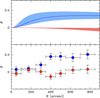 |
Fig. 6 Same as 4, but for anisotropy profile (see Sec. 3.2). |
| In the text | |
|
Fig. 7 Distribution of the three velocity components as a function of the position angle for MPs in 47 Tuc. Left and right panels refer to the FP and SP subpopulations, respectively. The solid lines show the best-fitting trend in all panels. |
| In the text | |
|
Fig. 8 2D density maps of stars selected in the GC 47 Tuc for kinematic analysis. FPs are shown in the left panel, while SPs in the right panel. Overplotted to the density distributions are the best-fit ellipses derived as described in Sect. 4. |
| In the text | |
|
Fig. 9 Bottom and middle panels show the distribution of the (α)LOS parameter for the FP and SP as a function of the dynamical age Nh for all clusters in the sample (gray circles). The upper panel shows the distribution of the rotation differences (αSP − αSP)LOS. The dashed lines represent the linear best-fit to the GC distribution. In all panels, the star symbols refer to the results obtained for the stacked analysis on the dynamically young (green) and old (orange) samples. The size of the star matches the amplitude of the errorbars. |
| In the text | |
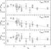 |
Fig. 11 As in Figs. 9 and 10, but now for the ω3D parameter (Sect. 5.1). |
| In the text | |
|
Fig. 12 Best-fit results of kinematic analysis of dynamically young (Nh < 8) and old (Nh > 8) stacked samples. FP is in red and SP in blue. The lower panels refer to the LOS rotation, while the upper row shows the results for the TAN velocity component. |
| In the text | |
|
Fig. 13 Distributions of (α)LOS parameter for FP and SP (lower and upper panel respectively) as a function of the best-fit ellipticity values (Sec. 4) for the two subpopulations. |
| In the text | |
|
Fig. 14 Time evolution of rotational parameters αFP, αSP, and their differences (see Sect. 5.1) for the simulations described in Sect. 5.3. The blue line corresponds to the model with δ = 0°; the pink, cyan, and purple correspond to δ = 45°, 90°, and 180°, respectively. |
| In the text | |
|
Fig. 15 Bottom and middle panels show the distribution of the anisotropy parameter αβ for the FP and SP subpopulations of GCs in the sample (gray circles) as a function of Nh. The top panel shows the differential trend |
| In the text | |
|
Fig. 16 Best-fit results of anisotropy analysis of MPs in the two stacked samples. The upper panel shows the best-fit anisotropy profiles of the FP (red) and SP (blue) subpopulations as obtained for the stacked sample of dynamically young GCs, while the lower panel refers to dynamically old systems. |
| In the text | |
|
Fig. 17 Time evolution of anisotropy parameters defined in Sec. 6.1 for the FP (bottom panel), the SP (middle panel), and their difference (top panel) in the three Monte Carlo simulations described in Sec. 6.2 (N1Mr10 blue line, N1M purple line; N05M pink line). Time is normalized by the half-mass relaxation time. |
| In the text | |
|
Fig. 18 Comparison between best-fit σ0, Arot, and Rpeak values obtained for MPs in the present work and by Martens et al. (2023). Blue dots refer to SP and red ones to FP results. |
| In the text | |
|
Fig. C.1 Distribution of the three rotation parameters defined in this work for the LOS, PM and 3D velocity components, as a function of the dynamical age (Nh) for the total population (TOT) of GCs in our sample. |
| In the text | |
|
Fig. C.2 Distribution of the (αTOT)LOS parameter for the total population as a function of the best-fit ellipticity values derived as described in Sect. 4. |
| In the text | |
|
Fig. C.3 Comparison between the best-fit σ0 and Arot values obtained for the TOT sample for the clusters in common between the present work and Bellazzini et al. (2012) – B12, Ferraro et al. (2018) – F18 and Petralia et al. (2024) – P24. |
| In the text | |
|
Fig. C.4 Left panel: Comparison with the best-fit σ0 values obtained by Baumgardt et al. (2019) − B19 – for the total population of GCs in common with the present work. Right panel: One-to-one comparison of the 3D rotation amplitude values A3D found by Sollima et al. (2019) – S19 – and the present analysis. |
| In the text | |
Current usage metrics show cumulative count of Article Views (full-text article views including HTML views, PDF and ePub downloads, according to the available data) and Abstracts Views on Vision4Press platform.
Data correspond to usage on the plateform after 2015. The current usage metrics is available 48-96 hours after online publication and is updated daily on week days.
Initial download of the metrics may take a while.