| Issue |
A&A
Volume 695, March 2025
|
|
|---|---|---|
| Article Number | A156 | |
| Number of page(s) | 12 | |
| Section | Galactic structure, stellar clusters and populations | |
| DOI | https://doi.org/10.1051/0004-6361/202453482 | |
| Published online | 18 March 2025 | |
The bulge globular cluster Terzan 6 as seen from multi-conjugate adaptive optics and HST★
1
Dipartimento di Fisica e Astronomia, Università degli Studi di Bologna,
Via Piero Gobetti 93/2,
40129
Bologna, Italy
2
INAF – Astrophysics and Space Science Observatory Bologna,
Via Piero Gobetti 93/3,
40129
Bologna, Italy
3
Departamento de Astronomia, Casilla 160-C,
Universidad de Concepcion, Chile
4
Departamento de Astronomía, Facultad de Ciencias, Universidad de La Serena.
Av. Juan Cisternas 1200,
La Serena, Chile
5
Universidad Andres Bello, Facultad de Ciencias Exactas, Departamento de Ciencias Físicas – Instituto de Astrofísica,
Autopista Concepcion-Talcahuano 7100,
Talcahuano, Chile
★★ Corresponding author; This email address is being protected from spambots. You need JavaScript enabled to view it.
Received:
17
December
2024
Accepted:
12
February
2025
Abstract
This work consists of the first detailed photometric study of Terzan 6, one of the least known globular clusters in the Galactic bulge. Through the analysis of high angular resolution and multiwavelength data obtained from adaptive optics corrected and space observations, we built deep, optical and near-infrared color-magnitude diagrams reaching ≈4 magnitudes below the main-sequence turnoff. Taking advantage of four different epochs of observations, we measured precise relative proper motions for a large sample of stars, from which cluster members have been solidly distinguished from Galactic field interlopers. A noncanonical reddening law (with RV = 2.85) and high-resolution differential reddening map, with color excess variations up to δE(B − V) ≈ 0.8 mag, have been derived in the direction of the system. According to these findings, new values for the extinction and distance modulus have been obtained: E(B − V) = 2.36 ± 0.05 and (m − M)0 = 14.46 ± 0.10 (corresponding to d = 7.8 ± 0.3 kpc), respectively. We also provide the first determinations of the cluster center and projected density profile from resolved star counts. The center is offset by more than 7″ to the east from the literature value, and the structural parameters obtained from the King model fitting to the density profile indicate that Terzan 6 is in an advanced stage of its dynamical evolution, with a large value for the concentration parameter (c = 1.94−0.26+0.24) and a small core radius (rc = 2.6−0.7+0.09 arcsec). We also determined the absolute age of the system, finding t = 13 ± 1 Gyr, in agreement with the old ages found for the globular clusters in the Galactic bulge. From the redetermination of the absolute magnitude of the red giant branch bump and the recent estimate of the cluster global metallicity, we find that Terzan 6 nicely matches the tight relation between these two parameters drawn by the Galactic globular cluster population.
Key words: Hertzsprung-Russell and C-M diagrams / stars: Population II / globular clusters: general / Galaxy: stellar content
Based on observations collected at the GEMINI South Observatory under program GS-2013A-Q23 (PI: Geisler), with the HST (GO14074, GO15616 and GO16420, PI:Cohen and Homan) and at the Very Large Telescope of the European Southern Observatory at Cerro Paranal (Chile) under Program 091.D-0115 (PI:Ferraro).
© The Authors 2025
 Open Access article, published by EDP Sciences, under the terms of the Creative Commons Attribution License (https://creativecommons.org/licenses/by/4.0), which permits unrestricted use, distribution, and reproduction in any medium, provided the original work is properly cited.
This article is published in open access under the Subscribe to Open model. This email address is being protected from spambots. You need JavaScript enabled to view it. to support open access publication.
1 Introduction
Galactic globular clusters (GCs) are populous and old stellar aggregates with typical ages of ∼12 Gyr (see e.g., Marín-Franch et al. 2009; VandenBerg et al. 2013; Valcin et al. 2020). They are considered powerful tracers of the early phase of the Milky Way (MW) formation, and their study provides crucial insights into the evolutionary history of our galaxy. The recent exploration of the Galactic halo performed by the Gaia mission (Gaia Collaboration 2016) has indeed demonstrated that the dominant fraction of GCs in the MW halo has an extra-Galactic origin, tracing the most relevant merging events (Gaia-Enceladus, Helmi stream, Sequoia, etc.) suffered by the MW over time. In this respect, the most famous example of a possible remnant of a remote merging event found in the Galactic halo is ω Centauri. Despite its original classification of a GC, this stellar system has been found to host multi-iron sub-populations (Norris et al. 1996; Origlia et al. 2003; Ferraro et al. 2004; Bellini et al. 2009, 2017; Villanova et al. 2014), and its properties suggest that it is the remnant of a nuclear star cluster of an accreted dwarf galaxy (Bekki & Freeman 2003).
However, the star clusters in the central portion of our galaxy, the bulge, still remain largely unexplored, due to the large extinction and crowding in its direction. However, the bulge contains about 25% of the total stellar mass of the MW and represents the first massive structure to have formed. Hence, understanding its structure and evolution and constraining the properties of its stellar populations is key to describing the formation and early evolutionary processes of the in situ Galaxy. Thanks to the recent development of the adaptive optics (AO) techniques in the near-infrared (NIR), a huge improvement in the knowledge of bulge GCs has been made (see e.g., Saracino et al. 2015, 2019). In this respect, recent studies (Ferraro et al. 2009, 2016, 2021) have shown that two stellar systems traditionally cataloged as bulge GCs, namely Terzan 5 and Liller 1, host populations with remarkable differences in age (Δt up to ~10–11 Gyr) and in iron abundance (Δ[Fe/H]~ 1 dex), and for these reasons, they might be the fossil remnants of more massive structures that contributed to the formation of the bulge (see also Lanzoni et al. 2010; Origlia et al. 2011, 2013, 2019; Massari et al. 2014, 2015; Pallanca et al. 2021; Dalessandro et al. 2022; Crociati et al. 2023; Alvarez Garay et al. 2024; Fanelli et al. 2024a). The discovery of their nature has further emphasized the urgency of an appropriate exploration of the GC population in the Galactic bulge.
In this exciting context, here we present a multiwavelength investigation of the poorly studied bulge GC Terzan 6, discovered by Terzan (1968) using Schmidt plates obtained at the Haute- Provence Observatory. It is located at longitude l= 358.571° and latitude b= −2.162° (Barbuy et al. 1997), at a distance of 1.3 kpc from the Galactic center and approximately 7 kpc from Earth (Valenti et al. 2007, see also Fahlman et al. 1995; Barbuy et al. 1997; Baumgardt & Vasiliev 2021). As illustrated in Fig. 1, it is located in the inner bulge, where the mean color excess is as high as E(B – V) = 2.35 (Harris 1996), and this is the main reason why it has been poorly investigated so far. Terzan 6 has an intermediate integrated luminosity (V -band absolute magnitude MV = −7.56; Harris 1996), with an estimated total mass of about 105M⊙ (Baumgardt & Hilker 2018), and it shows a very concentrated structure, suggesting that it is a possible post-core collapse system (Trager et al. 1995). It hosts two low-mass X-ray binaries that exhibit type-I X-ray bursts and sharp eclipse signals during outburst phases (see Painter et al. 2024; van den Berg et al. 2024, and references therein). While NIR low-resolution spectroscopy of CaII triplet (CaT) lines suggests [Fe/H]= −0.21 ± 0.15 (Geisler et al. 2023), recent high-resolution spectroscopic analysis of a sample of giants (Fanelli et al. 2024b) shows a metallicity of [Fe/H]= −0.65 for the stellar population hosted in the cluster.
Here we present the most detailed study so far of the stellar population hosted in Terzan 6, taking advantage of a combination of photometric data acquired through AO-assisted, ground-based facilities, and space-based instruments, which allowed the acquisition of images of superb quality and spatial resolution. This work is organized as follows. Section 2 describes the optical and the NIR data sets used in the analysis, and the adopted data analysis procedures. In Section 2.4 we present the derived optical, NIR, and hybrid color-magnitude diagrams (CMDs), and discuss the main characteristics of evolutionary sequences. Section 3 presents the relative proper motion (PM) analysis and the decontamination procedure adopted to remove the Galactic field interlopers, while Section 4 describes the method adopted to evaluate the extinction law and the differential reddening map in the direction of the cluster. In Section 5.1 we present a new determination of the center of gravity, projected density profile, and main structural parameters of the system, obtained from resolved star counts and King model fitting. Section 5.2 is focused on the determination of the distance modulus of Terzan 6 through a comparison with the CMD of the well-studied GC NGC 6624, and an estimate of its absolute age through isochrone fitting. We also show the position of Terzan 6 in the age-metallicity distribution drawn by bulge GCs. Section 5.3 is devoted to the determination of the absolute magnitude of the red giant branch (RGB) bump of the system. Finally, in Section 6 we present a summary of the work and the main conclusions.
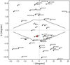 |
Fig. 1 Position in Galactic longitude (l) and latitude (b) of the known GCs in the direction of the bulge (from the Harris 1996 compilation). For reference, the black lines represent the outline of the inner bulge. The position of Terzan 6 is shown as a large red circle. |
2 Observations and data analysis
2.1 Optical and NIR data sets
The photometric investigation of Terzan 6 presented in this study combines optical and NIR datasets. In the following we schematically present the adopted datasets. The optical photometric data set is composed of high-resolution, multi-epoch images obtained from the Wide Field Channel (WFC) of the Advanced Camera for Survey (ACS) on board Hubble Space Telescope (HST). The WFC/ACS provides ~0.05 arcsec/pixel spatial resolution in a nominal 202 × 202 arcsec2 field of view (FoV). In particular, the analyzed optical data set is composed of images acquired in three different epochs. The first epoch was acquired in 2016 (Proposal ID. 14074 P.I Cohen) and comprises images obtained only in the F606W filter. The second one was performed in 2019 (Proposal ID. 15616 P.I. J. Homan), while the third one in 2021 (Proposal ID. 16420 P.I. J. Homan). They are both composed of images obtained in the F606W and F814W filters. For the sake of illustration, Fig. 2 shows the portion of an image (in the F814W filter) containing the central region of the cluster.
The NIR data set consists of a set of high-resolution images obtained in 2013 with the Gemini South Adaptive Optics Imager (GSAOI) assisted by the Gemini Multi-Conjugate Adaptive Optics System (GeMS), mounted at the 8m Gemini South Telescope. The GSAOI camera is a 4k × 4k NIR imager covering 85″ × 85″ designed to work at the diffraction limit of the 8- meter telescope with a spatial sampling of 0.02″/pixel. The analyzed data set is part of the GEMINI program GS-2013A-Q23 (P.I D. Geisler) and it is composed of a set of 23 images in the J filter and 20 in the Ks filter. Figure 3 shows a Ks-band image of the GSAOI chip containing the central region of cluster. For photometric calibration purposes, the Gemini images were complemented by HAWK-I (High Acuity Wide field K-band Imager) observations in the K and J bands acquired in 2013 (Proposal ID. 091.D-0115(B) P.I F.R. Ferraro) at the Very Large Telescope. HAWK-I is a wide-field NIR imager that covers 7.5′ × 7.5′ in the sky with a pixel scale of 0.106″/pixel. Fig. 4 shows the FoV covered by the different datasets and Table 1 summarizes all the exposures analyzed in the present study.
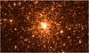 |
Fig. 2 (60″ × 35″) portion of a WFC/ACS image centered on Terzan 6 obtained in F814W with an exposure time of 473 s. North is up, east is to the left. |
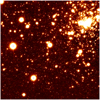 |
Fig. 3 (40″ × 40″) image of Terzan 6 obtained in the Ks filter of GSAOI with an exposure time of 30s. North is up, and east is to the left. |
2.2 Data reduction
For the NIR data set, we performed the prereduction procedure individually for each of the four chips, by using standard IRAF1 tools to correct for bias and flat field and to perform the sky subtraction (imcombine and flatcombine to combine the different sky and flat images respectively, ccdproc to apply the correction to the different scientific images). To estimate the unresolved background we combined the target scientific images in order to build a MASTER SKY. For the images secured with HAWK- I the prereduction procedure has been performed by using the EsoReflex software (Freudling et al. 2013), with the specific HAWK-I pipeline. The evaluated full-width at half maximum (FWHM) is ≈400 mas for the K-band image and ≈450 mas for the J ones.
As for the HST data, we used _flc images, which are already calibrated and corrected for the Charge Transfer Efficiency (CTE). In addition these images are already processed by the Space Telescope Institute dedicated pipeline and are corrected for bias and flat-fielding effects. We applied the Pixel Area Map corrections by exploiting the time-averaged files available on the ACS website2.
For both optical and NIR data the photometric reduction procedure was performed independently for each chip, filter, and epoch. The photometric analysis of the images was performed by point spread function (PSF)-fitting since this approach allows the derivation of accurate measures of the source luminosities even in the case of a high level of crowding, as in the case of the central regions of a GC. To this aim, we made use of the DAOPHOT (Stetson 1987) software. We used a sample of bright, isolated, and uniformly distributed stars to model the PSF using the DAOPHOT/PSF routine and allowing a cubic polynomial spatial variation. The analysis of the PSF for the NIR dataset allowed us to perform a quality check of all the acquired images. Thus, the 18 J-band images (with mean FWHM ≈150 mas) and 13 Ks-band images (with mean FWHM ≈80 mas) acquired in the best observational conditions have been selected for the PSF fitting analysis. The obtained PSF models were then applied to all star-like sources detected at 4σ (for GEMINI and HAWK-I) and 5σ (for HST) above the background level using ALLSTAR. At this point, for each image, we had a list with instrumental coordinates, magnitudes, and relative errors for the detected stars. We used it to create a combined master star list for HST and GEMINI, which included all the stars measured in at least one image. Following the approach of previous studies (e.g., Dalessandro et al. 2014, and references therein), this master list was used as input for ALLFRAME (Stetson 1994), which was performed independently for each chip and epoch. The resulting output files were then combined to generate a catalog containing all the stars detected in more than half of the images (per chip and filter), using as reference the WFC1 HST’s 2021 epoch, which covers the cluster’s center. This criterion removed the vast majority of spurious detections (such as those due to cosmic rays etc). For each stellar source in the catalogs, the various magnitude estimates were homogenized. The mean values and standard deviations of these estimates were then assigned as the star magnitudes and photometric errors in the final catalog (Ferraro et al. 1991, 1992).
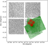 |
Fig. 4 FoVs of the data sets analyzed in this study: the HAWK-I’s FoV (7.5′ × 7.5′) is plotted in gray, the FoV of the different HST/WFC/ACS pointings is in green, and that of GeMS is in red. |
Summary of the data sets used.
2.3 Astrometry and calibration
The next necessary step to build the final catalog was to transform the instrumental coordinates to the absolute reference frame (α and δ) and to perform the photometric calibration of the magnitudes. First of all, it was essential to correct the instrumental coordinates for the effects of geometric distortions. To this aim, we followed Bellini et al. (2011) for ACS-WFC, while for the GeMS/GSAOI camera, we applied the solutions provided by Dalessandro et al. (2016). The astrometric transformation of the catalog has been performed by using the stars in common with the publicly available Gaia DR3 catalog (Gaia Collaboration 2023) and through the cross-correlation software CataXcorr (Montegriffo et al. 1995).
HST magnitudes were reported to the VEGAMAG photometric system, utilizing the zero points and the encircled energy fraction provided on the ACS website for a 1″ (20 pixels) aperture and performing the aperture correction. The J and Ks instrumental magnitudes have been reported to the 2MASS photometric system by using the Vista Variables in the Via Lactea (VVV) catalog (Smith et al. 2018). However, since the number of stars in common between the GEMINI catalog and VVV is quite low, we used the ESO/HAWK-I images to derive a sort of “bridge catalog” to report the J and Ks magnitude of the GEMINI catalog in the VVV system. As shown in Fig. 4 the GeMS FoV is entirely contained in just one HAWK-I chip (Chip 2), thus the HAWK-I catalog has been cross-correlated with the VVV one and finally used to calibrate the GeMS magnitudes.
2.4 NIR and Optical CMDs of Terzan 6
Fig. 5 shows the CMDs obtained from the analyzed observations in different filter combinations. In particular panel (a) shows the (mF814W, mF606W – mF814W) optical CMD, panel (b) the (Ks, J-Ks)-CMD in the pure NIR bands, and panel (c) the hybrid optical-NIR (mF814W, mF814W – Ks) CMD. The evolutionary sequences can be well identified in all the diagrams. It is possible to distinguish the red clump at Ks ≈ 14 (J ≈ 15.5, mF814W ≈ 18.5, mF606W ≈ 21), a well-extended RGB with the RGB-bump clearly visible at Ks ≈ 14.5 and mF814W ≈ 19, and the Sub-Giant Branch (SGB). The CMD extends to more than ≈4 mag below the Main Sequence Turn Off (MS-TO), which is clearly visible at mF814W ≈ 22 (Ks ≈ 17.5). The comparison of the CMDs shown in Fig. 5 with previous results published in the literature (Figure 2 of Fahlman et al. 1995; Figure 2 of Valenti et al. 2007) allows to fully appreciate the advantages of using of multi-conjugate AO systems (such as the GeMS/GSAOI system), which are able to provide results comparable to those obtainable from space (see Figure 18 of Cohen et al. 2018).
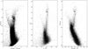 |
Fig. 5 (mF814W, mF606W – mF814W), (Ks, J – Ks), and (mF814W, mF814W – Ks) observed CMDs of Terzan 6 obtained from the analysis of the HST and GeMS images discussed in the text. The small red crosses in the right-hand side of each panel show the photomeric errors at different magnitude levels. |
3 Proper motion analysis
The characterization of the evolutionary sequences requires an appropriate decontamination of the CMD from galactic field interlopers. This is particularly critical in the case of bulge GCs because they are heavily embedded into the bulge, thus a non- negligible fraction of the sources detected along the line-of-sight are likely field stars. In particular, we exploited the large temporal baseline provided by the multi-epoch data set (see Table 1) to perform an accurate relative PM analysis. We used different temporal baselines depending on how many (two, three or four) observations of the same star are available in the datasets. For this analysis we used the approach described in Dalessandro et al. (2013, see also Massari et al. 2013; Bellini et al. 2014; Massari et al. 2015; Cadelano et al. 2022, 2023) and to avoid saturation problems we considered stars with mF814W > 16. Briefly, the procedure consists of determining the displacement of the centroids of the stars measured in two or more epochs once a common coordinate reference frame is defined. The first step is to adopt a distortion-free reference frame, hereafter “master frame.” The master-frame catalog contains stars measured in all the ACS/WFC F814W-band single exposures secured in 2021 (third HST epoch). To derive accurate geometrical transformation between our catalog and the master frame we selected a sample of ≈3000 bona-fide stars uniformly distributed in the FoV and distributed along the RGB and the red clump at magnitudes 17 < mF814W < 20 and colors 2.50 < (mF606W – mF814W) < 3.50, to maximize the membership probability. The mean position of a single star in each epoch has been measured as the (ɜσ–)clipped mean position calculated from all the N individual single-frame measurements. The relative rms of the position residuals around the mean value divided by N has been used as the associated error (σ). Finally, the displacements are obtained as the positional differences among the different epochs. The error associated with the displacement is the combination of the errors on the positions in each epoch. The relative PMs (µx, µy) are finally determined by measuring the difference of the mean x and y positions of the same stars in the different epochs, divided by their temporal baseline ∆t. Such displacements are in units of pixels yr−1 . In the case of three or more epochs, we evaluated the PMs as the angular coefficients of the relation between the x and y positions and the time, expressed in Julian Day (JD).
We then iterated this procedure a few times by removing likely nonmember stars from the master reference frame based on the preliminary PMs obtained in the previous iterations. The convergence is assumed when the number of reference stars that undergo this selection changes by less than ≈10% between two subsequent steps.
As result, we derived relative PMs for 135134 stars. In particular, we computed relative PMs by using only two different epochs for 71201 stars; while for 53118 stars we exploited three different epochs, and finally 10815 stars were observed in four different epochs. To build a clean sample of stars with a high membership probability, we constructed the vector-point-diagram (VPD) in five magnitude bins with a width of two mag each (see Fig. 6d) As expected, the PM distributions get broader for increasing magnitudes because of the increasing uncertainties in the centroid positions of faint stars. By definition in each magnitude bin, cluster stars are expected to be distributed around position (0,0), and we adopted as likely cluster members all the stars included within 3σ from this value, where σ is the average PM error in that magnitude bin. The CMD of the member stars selected according to this criterium is shown in Fig. 6c, while that of Galactic field interlopers is plotted in Fig. 6b. As clearly visible (especially in the top panels of Fig. 6d), the PM of the bulge field and disk stellar populations describe a vaguely elliptical broad distribution extending toward positive values of Δx and Δy. This distribution partially overlaps the portion of the VPD where cluster members are selected, thus some residual contamination is expected in the PM-cleaned CMDs. Nevertheless, we can notice that all the evolutionary sequences are much better defined in the PM-cleaned CMD (Fig. 6c). This also demonstrates that ground-based AO observations can be successfully combined with HST observations to perform a reliable PM analysis even in dense environments (see also Saracino et al. 2019; Ferraro et al. 2021; Dalessandro et al. 2022).
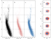 |
Fig. 6 Panel a: hybrid CMD of all the stars in common between GEMINI and at least one of the HST epochs. Panel b: CMD of the likely field interlopers according to the PM analysis. Panel c: CMD of the likely cluster members according to the measured PMs. Panel d: VPDs of the measured stars. The circles have a radius equal to 3σ, with σ being the average PM error in each magnitude bin. The blue (red) dots within (beyond) the circles are classified as cluster members (field interlopers) and their CMD is plotted in panel c (panel b). |
4 Differential reddening
Because of the position of Terzan 6 in the bulge of the Galaxy, at only about 1 kpc from the Galactic center, one of the most severe challenges in its characterization is represented by the huge and differential interstellar absorption along the line of sight, due to the presence of clouds with different column densities on scales that can be as small as a few arcseconds (see, e.g., Pallanca et al. 2021). This implies that, depending on its location in the acquired image, each star is affected by a different color excess E(B – V), which is defined as the difference between the observed color (B – V) and the intrinsic one (B – V)0. The main resulting effect on the CMD is an elongation of the main evolutionary features along the direction of the reddening vector, an effect that is commonly referred to as differential reddening. To correct the observed sample for differential reddening we proceeded in two steps: STEP1 – the identification of the direction of the reddening vector in the adopted CMDs; STEP2 – the operative star-by-star correction.
STEP1 – The direction of the reddening vector depends (through the wavelength-dependent parameters commonly named Rλ) on the photometric filters used to build the CMD. These parameters are linked to the extinction coefficient Aλ through Aλ = Rλ × E(B − V), and they can be expressed as the product of two terms:  . The coefficient
  is therefore equal to the ratios Aλ/AV and Rλ/RV, which express the wavelength dependence of interstellar extinction relative to the absolute extinction in the V -band, and are commonly referred to as “reddening law” (see, e.g., Cardelli et al. 1989; Fitzpatrick & Massa 1990; O’Donnell 1994; Fitzpatrick 1999). The V -band extinction coefficient RV is usually assumed to be 3.1, which is the standard value for diffuse interstellar medium (Schultz & Wiemer 1975; Sneden et al. 1978), but it has been observed to vary along different directions toward the inner Galaxy (Popowski 2000; Nataf et al. 2013b; Casagrande & VandenBerg 2014; Alonso-García et al. 2017; Pallanca et al. 2021, and references therein). This implies that the reddening law can be steeper or shallower along different lines of sight, because the wavelength dependence of
  changes with the adopted value of RV (see, e.g., Fig. 3 of Cardelli et al. 1989 or Fig. 3 in Pallanca et al. 2021). Thus, to determine the value of RV along the line of sight of Terzan 6, we selected a sample of stars along the bluest side of the RGB in the optical CMD, and another sample along the reddest RGB envelope. Then, we adopted different values of RV and, for each of them, we shifted the red sample along the corresponding direction of the reddening vector until it matched the blue sample. This has been done in both the optical and the NIR CMDs, each time measuring the amount of shift needed to superpose the two samples. We found that the best superposition of the two samples in the optical and the NIR CMDs simultaneously, implying approximately the same values of E(B − V) needed in the two shifts, is obtained3 for RV = 2.85. The corresponding values of Rλ in the photometric filters of interest for our study therefore are: RF606W = 2.64, RF814W = 1.70, RJ = 0.79, and
  .
.
STEP2 – Once the appropriate extinction law has been set, to correct the CMDs we adopted the so-called star-by-star approach, which is described in detail by Pallanca et al. (2019, see also Cadelano et al. 2020a). In summary, in the optical HST CMD we first determined the mean ridge line (MRL) of Terzan 6 using a sample of well-measured and likely member stars located along the RGB, SGB, and bright MS. Then, for each star in our HST catalog, we selected a group of nearby (within a limiting radius of 10″), well-measured stars (N*) to create a “local CMD.” By progressively shifting the MRL along the direction of the reddening vector, in steps of δE(B − V), we evaluated the residual color ΔVI as
 (1)
(1)
where VIobs,i is the (V − I) color for each of the N* stars of the local CMD, VIMRL,i is that of the MRL at the same level of magnitude, and the weight wi depends on both the photometric error on the color (σ) and the spatial distance (d) of the ith source from the considered star. So the final value of δE(B − V) assigned to each star is the one which minimizes the residual color (ΔVI/N*).
These values have been used to build the differential reddening map in the direction of Terzan 6, over a FoV of about 200″ × 200″, roughly corresponding to the FoV covered by the HST observations, with an angular resolution of only a few 0.1″. The derived differential reddening map is shown in Fig. 7. As can be appreciated from the figure the reddening appears patchy on spatial scales of just a few arcseconds, with a highly reddened blob (dark color in the figure) located in the southeastern region of the cluster. Another highly reddened structure can be distinguished diagonally crossing the northwestern corner of the FoV as a sort of thin strip. Less absorbed regions (lighter color in the figure) are located in the southwest and the east portion of the cluster. Overall, the map graphically indicates a large amount of differential reddening, with δE(B − V) ranging between −0.4 and 0.4. This corresponds to variation of differential absorptions of 2.1, 1.36, 0.63, and 0.26 mag in the V, I, J, and K filters, respectively. The obtained reddening map has been used to correct the effect of the differential reddening from the observed CMDs.
The PM-selected and differential reddening-corrected optical CMD is shown in Fig. 8. The effect of the correction for differential reddening is clearly visible, especially at the level of the red clump and the RGB bump, which both appear strongly elongated in the reddening direction non-corrected CMD. In the following analyses, the adopted magnitudes are always corrected for differential reddening.
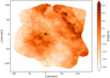 |
Fig. 7 Differential reddening map relative to the cluster center position (black cross, see Sect. 5.1) of the portion of the HST FoV where it was possible to derive a reliable correction. North is up, and east is to the left. Darker colors correspond to more extincted regions, as detailed in the side color bar. |
5 Results
5.1 Center, density profile, and structural parameters
The first step for the determination of the density profile is the estimate of the system’s center of gravity (Cgrav). In this case it has been derived by using resolved star counts, thanks to the high spatial resolution of the data used for the analysis. With respect to integrated light studies, resolved star counts offer the main advantage of avoiding observational biases generated by the possible presence of a few bright stars that can offset the surface brightness peak from the true center position. To determine Cgrav we calculated the barycenter position of the stars selected within a given magnitude range and within a given radial distance, starting from a first-guess center (Harris 1996). Then, the procedure is iteratively repeated by adopting as new center the barycenter position calculated in the previous step, and convergence is reached when the difference between two successive estimates is smaller than 0.01″ (see, e.g., Montegriffo et al. 1995; Miocchi et al. 2013). The analysis was performed on stars selected with five radial distances (namely, 5, 10, 15, 20, 25 arcsec) and three faint magnitude limits (mF814W < 21,21.5,22), thus providing 15 values of converge. The choice of the radial distances is set so that a gradient in the cluster density profile is sampled. A decrease of the density profile starts to be detectable around the core radius (rc), hence the confidence radii have been chosen larger than the literature value of rc (namely, 3″; Harris 1996). The faint magnitude limits are chosen to avoid spurious fluctuations due to photometric incompleteness, and we also adopted a bright cut (at mF184W = 16) to exclude stars affected by saturation problems. The adopted magnitude limits also guarantee that the stars selected for the center’s determination have approximately the same mass. The final result is obtained by averaging the 15 barycenter positions, and the associated error is the standard deviation of the mean. The obtained coordinates of Cgrav are αJ200 = 17h50m46.9s, δJ200 = −31° 16′ 30.56″, with an error of 0.44" on α and 0.18″ on δ. The new determination of the cluster center is very different from the one reported in the literature: it is located at ≈7″ from the one quoted in Harris (1996), toward the east and just ~0.8″ to the north.
Once Cgrav has been obtained, we determined the radial density profile from resolved star counts (see, e.g., Miocchi et al. 2013, for a detailed description of the procedure). We split the FoV into concentric rings of different sizes chosen to ensure good statistics, and we determined the star density (number of stars divided by the ring area) within each of them. To avoid incompleteness problems, only stars with mF814W < 20.8 have been used. The projected density profile resulting from this operation is shown in Fig. 9 through empty circles. In the outermost regions, at about r > 50″ , we note a flattening, with density values that remain constant at about −1.13 stars arcsec−2, due to the contribution of Galactic field stars. We determined the average level of the background as the mean of the densities of the three outermost rings. This value was subtracted from the observed profile, thus providing the true radial density distribution of the cluster (see the black circles in Fig. 9). As expected, the field decontamination significantly affects the external portion of the profile, leaving the central one essentially unchanged.
To estimate the structural parameters of Terzan 6, we followed the procedure explained in Raso et al. (2020, see also Giusti et al. 2024; Deras et al. 2024, 2023; Pallanca et al. 2023). It consists of a Monte Carlo Markov Chain (MCMC) fitting of the observed profile with King (1966) models, assuming flat priors for the fitting parameters (namely the central density, the King concentration parameter c, and rc) and a χ2 likelihood. The best-fit profile thus derived is shown in Fig. 9. It is characterized by  , which corresponds to a dimensionless central potential
  , half-mass radius
  arcsec, and tidal radius
  arcsec. The core radius is well consistent with that quoted in Harris (1996, rc = 3″). The concentration parameter is smaller than the literature one (c = 2.5 in Harris 1996), but still indicates an advanced stage of internal dynamical evolution for this cluster.
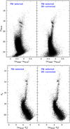 |
Fig. 8 Optical (upper panels) and hybrid (bottom panels) CMD of the PM-selected member stars before (left panels) and after (right panels) the correction for differential reddening (DR in the plot). |
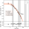 |
Fig. 9 Projected density profile of Terzan 6 derived from star counts in concentric annuli around Cgrav (empty circles). The horizontal dashed line indicates the Galactic field density, which has been subtracted from the observed points (empty circles) to obtain the background-subtracted profile, shown as filled circles. The red solid line represents the best-fit King model to the cluster’s density profile, with the red stripe indicating the ±1σ range of solutions. The vertical lines denote the positions of the core radius (dashed line), half-mass radius (dot-dashed line), and tidal radius (dotted line), with their respective 1σ uncertainties highlighted by gray stripes. The values of the main structural parameters obtained from the fitting process are also labeled (see details in the text). |
5.2 Distance, reddening, and age
We obtained a first estimate of the distance modulus and mean color excess of Terzan 6 through the comparison with NGC 6624, a well-studied GC of similar metallicity ([Fe/H]= −0.69; Valenti et al. 2011) with well-constrained foreground extinction E(B − V) = 0.28 and true distance modulus (m − M)0 = 14.50 ± 0.10 (Harris 1996, see also Saracino et al. 2016 and Baumgardt & Vasiliev 2021). To this aim, we shifted the PM- selected and differential reddening corrected CMD of Terzan 6 onto that of NGC 6624 reported into the absolute plane. We found that the optimal match is obtained by adopting E(B − V) = 2.37 ± 0.05 and a true distance modulus (m − M)0 = 14.45 ± 0.15 (see Figure 10) Starting from these first-guess values, we then refined both the estimates and determined the age of Terzan 6 via isochrone fitting of the differential reddening corrected and PM- selected hybrid (Ks, mF814W − Ks) CMD, which provides the best compromise between large wavelength baseline and good photometric accuracy at the level of the MS-TO. We also limited the analysis to the stars sampled in the radial range 5″ < r < 25″, which optimize the definition of the MS-TO region. The theoretical models used for this analysis are the BASTI (Pietrinferni et al. 2004) and the PARSEC (Bressan et al. 2012) isochrones4. We assumed [Fe/H]=−0.65, [α/Fe]= 0.4, and helium abundance Y=0.247, and used models also including overshooting and mass loss along the RGB (see Origlia et al. 2002, 2007). We retrieved models calculated for ages ranging between 10 to 14 Gyr in both the ACS/WFC and the 2MASS photometric systems. To find the best matching of the isochrones with the data we allowed the distance modulus and the reddening to vary within the 1-σ error of the estimated first-guess values. The result of this iteration is plotted in Fig. 11, showing the BASTI and the PARSEC isochrones that best reproduce simultaneously the Horizontal Branch (HB) level (left panels) and the MS-TO region (right panel). Slightly different values of the distance modulus, reddening, and age are required to optimize the match between the two sets of isochrones and the data: (m − M)0 = 14.53 ± 0.1, E(B − V) = 2.38 ± 0.05, and t = 12.5 ± 1 Gyr for the PARSEC isochrones, (m − M)0 = 14.43 ± 0.1, E(B − V) = 2.33 ± 0.05, and t = 13.5 ± 1 Gyr for the BASTI models. Thus, we assumed the average values as final estimates of these parameters for Terzan 6, obtaining a true distance modulus (m − M)0 = 14.46 ± 0.10 (d = 7.8 ± 0.3 kpc), a color excess E(B − V) = 2.36 ± 0.05, and an age t = 13 ± 1 Gyr, with conservative estimates of the associated errors. The derived distance modulus appears to be larger than the literature values: (m − M)0 = 14.11 (Harris 1996), (m − M)0 = 14.16 ± 0.14 (Fahlman et al. 1995), (m − M)0 = 14.25 (Barbuy et al. 1997), (m − M)0 = 14.13 (Valenti et al. 2007). However, it is important to notice that those works assumed RV = 3.12, while here we are using the new determination (RV = 2.85) discussed in Section 4. In terms of distance, our result is compatible within the errors with the mean of the literature values,  (Baumgardt & Vasiliev 2021).
By exploiting the information about the age and the metallicity of the system, we can place Terzan 6 in the age-metallicity diagram (Fig. 12), together with other bulge GCs. We can notice that the position of Terzan 6 is fully compatible within the errors with the average age of bulge GCs, confirming an insitu origin of this system (as already dynamically proved by Massari et al. 2019).
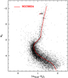 |
Fig. 10 CMD of Terzan 6 in the absolute plane (black dots), with the MRL of NGC 6624 superposed as a red line. |
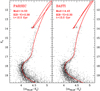 |
Fig. 11 Differential reddening-corrected and PM-selected (Ks , mF814W − Ks) CMD of Terzan 6 with over-plotted the isochrones that best reproduce simultaneously the HB level and the MS-TO, for the PARSEC and the BASTI models (left and right panel, respectively). The values of the distance modulus, reddening, and age required to optimize the match with the data are also labeled. |
5.3 The RGB bump
One of the most relevant evolutionary features characterizing the RGB is the so-called RGB bump. It flags the star luminosity at the moment when the hydrogen-burning shell crosses the hydrogen discontinuity left by the innermost penetration of the convective envelope (see Fusi Pecci et al. 1990; Ferraro et al. 1991, 1992, 1999, 2000; see also the compilations by Zoccali et al. 1999; Valenti et al. 2004, and more recently by Nataf et al. 2013a). Hence, the predicted luminosity of the RGB bump depends on all the parameters and physical processes affecting the penetration of convection deep into the stellar interior (for instance, the parameters affecting stellar opacity, such as the heavy element and helium abundances). In the case of a deep penetration, the hydrogen-burning shell is expected to cross the chemical discontinuity left by the convective envelope at an early stage of the RGB evolution, and the bump occurs at faint magnitudes along the RGB. Thus, a strong dependence is expected between the RGB bump luminosity and the overall metallicity of the stellar population. From the observational point of view, the RGB bump can be easily identified via the detection of a local increase of star counts (a “bump in star counts”) along the RGB differential luminosity function (e.g., Fusi Pecci et al. 1990; Ferraro et al. 1999, 2000), due to a temporary hesitation in the star evolutionary path when crossing the hydrogen discontinuity.
The high-quality CMDs obtained in this study offer the possibility to identify this feature in Terzan 6. Indeed, already from a visual inspection of Fig. 8, the location of the RGB bump is easily recognizable in the CMD as a small clump of stars along the RGB at slightly lower luminosity than the red clump. Fig. 13 shows the RGB differential luminosity function in different filters obtained from the PM-selected and differential reddening corrected CMDs shown in Fig. 8. The RGB bump is located at mF606W = 21.80 ± 0.05, mF814W = 19.00 ± 0.05, J = 16.05 ± 0.05, and Ks = 14.50 ± 0.05.
Adopting the color excess and distance modulus derived in Section 5.2, the absolute magnitude of the RGB bump is MF606W = 1.16 ± 0.12, MF814W = 0.59 ± 0.12, MJ = −0.20 ± 0.12, and  . As pointed out by Ferraro et al. 1999, to evaluate the dependence of the RGB bump luminosity on the metallicity, one must consider the global metallic- ity ([M/H]), which includes the contribution from α-elements and can be estimated from the relation (Salaris et al. 1993): [M/H]=[Fe/H] + log(0.638 × fα + 0.362), where fα = 10[α/Fe]. Thus, assuming [Fe/H]=−0.65 and [α/Fe]= 0.4, for Terzan 6 we obtain [M/H]= −0.34. In Fig. 14 we show the comparison among the value obtained here for Terzan 6 to those derived for other Galactic GCs in the literature (Nataf et al. 2013a; Pallanca et al. 2021; Deras et al. 2024), in the V – and NIR bands. Indeed, the Terzan 6 determinations nicely fit into the relations defined by previous works.
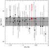 |
Fig. 12 Age–metallicity distribution for the bulge GCs from the literature (black symbols) and for Terzan 6 (large red square). The literature data are mainly from Saracino et al. (2019, see their Figure 16), Oliveira et al. (2020, see their Figure 12), and Cohen et al. (2021), with the addition of a few recent age determinations for NGC 6440 (Pallanca et al. 2021), NGC 6256 (Cadelano et al. 2020b), and NGC6316 (Deras et al. 2023). The age and metallicity of the oldest stellar population in the two suspected bulge fossil fragments (namely, Terzan 5 and Liller 1; Ferraro et al. 2009, Ferraro et al. 2021) are plotted as black triangles. The gray vertical strip marks the weighted average and the 1σ uncertainty (12.6 ± 0.6 Gyr) of the entire sample. |
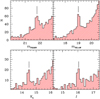 |
Fig. 13 Differential luminosity function of RGB stars classified as cluster members. The detected peaks (marked by vertical black segments) are the RGB bump in the four photometric bands (see labels). |
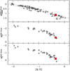 |
Fig. 14 Absolute magnitude of the RGB bump in the mF606W, K, and J bands (from top to bottom) as a function of the cluster global metal- licity [M/H]. The small gray squares are data from the literature: in the upper panel from Nataf et al. (2013a); Pallanca et al. (2021); Deras et al. (2024), in the central and bottom panels from Valenti et al. (2004, 2007); Pallanca et al. (2021). In all the panels the large red squares mark the location of the RGB bump estimated here for Terzan 6. |
6 Summary and conclusions
This work is set in the framework of using GCs as excellent tracers of the early stages of the formation and evolution of the MW. In particular, it is part of a larger project aimed at obtaining a detailed photometric (Saracino et al. 2015, 2016, 2019; Deras et al. 2023, 2024; Pallanca et al. 2019, 2021; Cadelano et al. 2020a, 2023; Ferraro et al. 2023), chemical (Crociati et al. 2023; Fanelli et al. 2024a,b; Alvarez Garay et al. 2024), kinematic (Leanza et al. 2023; Pallanca et al. 2023; Libralato et al. 2022; Ferraro et al. 2018), and chronological characterization of the population of Galactic bulge clusters, which have been poorly studied so far because of the large foreground extinction and stellar density. To overcome these limitations, we used a combination of high-resolution, multi-epoch NIR and optical data sets acquired with GeMS/GSAOI at GEMINI and with the ACS/WFC onboard the HST. Thanks to the high angular resolution offered by both data sets, and to the NIR sensitivity of the GeMS@GEMINI, it has been possible to perform the first detailed study of the stellar population hosted in the heavily reddened GC Terzan 6. The derived CMDs span ≈10 magnitudes, allowing us to observe all the main evolutionary sequences from the red clump level, down to ≈3 mag below the MS-TO. Thanks to the multi-epoch data set and the large temporal baseline, it was possible to derive relative PMs for 135 134 stars in this highly contaminated stellar system. To do this, we exploited all three HST epochs and the GEMINI epoch. In particular, we computed the relative PMs by using two different epochs for 71 201 stars, three different epochs for 53 118 stars, and all four different epochs for 10 815 stars. This analysis enabled a clear separation between cluster members and stars belonging to the Galactic field, thus making possible a detailed characterization of the stellar population of the system. Then, we obtained a high-resolution differential reddening map in the direction of the cluster, finding that δE(B − V) varies by ≈0.8 mag in the FoV of our data sets. The reddening law in the direction of the system is noncanonical, with RV = 2.85. By using the sky positions of resolved stars, we obtained a new estimate of the center of the system, finding that it is very different (i.e., offset by ~7″ to the east with respect to the one quoted in the literature and obtained through surface brightness studies; Terzan 1971; Harris 1996). We also determined the very first projected density profile obtained from resolved star counts. The analysis presented here indicates that Terzan 6 has experienced or is on the verge of experiencing the collapse of the core. By taking advantage of the PM-selected and differential reddening corrected CMDs, we estimated that Terzan 6 is located at a distance d = 7.8 ± 0.3 kpc from the Sun, and has an absolute age t = 13 ± 1 Gyr.
In summary, this work allowed the characterization of the stellar population properties of the bulge GC Terzan 6 with a level of detail never reached before. It also shows the wealth of information that it is possible to obtain even in high-density and large extinction regions such as the Galactic bulge, from the combination of NIR adaptive optics supported systems and optical space-based instruments.
Data availability
The photometric catalog is available at the CDS via anonymous ftp to cdsarc.cds.unistra.fr (130.79.128.5) or via https://cdsarc.cds.unistra.fr/viz-bin/cat/J/A+A/695/A156
Acknowledgements
This work is part of the project Cosmic-Lab at the Physics and Astronomy Department “A. Righi” of the Bologna University (www.cosmic-lab.eu/Cosmic-Lab/Home.html). M.L. acknowledges funding from the European Union NextGenerationEU. D.G. gratefully acknowledges the support provided by Fondecyt regular n. 1220264. D.G. also acknowledges financial support from the Dirección de Investigación y Desarrollo de la Universidad de La Serena through the Programa de Incentivo a la Investigación de Académicos (PIA-DIDULS). S.V. gratefully acknowledges the support provided by Fondecyt Regular n. 1220264 and by the ANID BASAL project ACE210002.
References
- Alonso-García, J., Minniti, D., Catelan, M., et al. 2017, ApJ, 849, L13 [Google Scholar]
- Alvarez Garay, D. A., Fanelli, C., Origlia, L., et al. 2024, A&A, 686, A198 [NASA ADS] [CrossRef] [EDP Sciences] [Google Scholar]
- Barbuy, B., Ortolani, S., & Bica, E. 1997, A&AS, 122, 483 [NASA ADS] [CrossRef] [EDP Sciences] [Google Scholar]
- Baumgardt, H., & Hilker, M. 2018, MNRAS, 478, 1520 [Google Scholar]
- Baumgardt, H., & Vasiliev, E. 2021, MNRAS, 505, 5957 [NASA ADS] [CrossRef] [Google Scholar]
- Bekki, K., & Freeman, K. C. 2003, MNRAS, 346, L11 [Google Scholar]
- Bellini, A., Piotto, G., Bedin, L. R., et al. 2009, A&A, 507, 1393 [NASA ADS] [CrossRef] [EDP Sciences] [Google Scholar]
- Bellini, A., Anderson, J., & Bedin, L. R. 2011, PASP, 123, 622 [CrossRef] [Google Scholar]
- Bellini, A., Anderson, J., van der Marel, R. P., et al. 2014, ApJ, 797, 115 [Google Scholar]
- Bellini, A., Milone, A. P., Anderson, J., et al. 2017, ApJ, 844, 164 [NASA ADS] [CrossRef] [Google Scholar]
- Bressan, A., Marigo, P., Girardi, L., et al. 2012, MNRAS, 427, 127 [NASA ADS] [CrossRef] [Google Scholar]
- Cadelano, M., Saracino, S., Dalessandro, E., et al. 2020a, ApJ, 895, 54 [NASA ADS] [CrossRef] [Google Scholar]
- Cadelano, M., Chen, J., Pallanca, C., et al. 2020b, ApJ, 905, 63 [NASA ADS] [CrossRef] [Google Scholar]
- Cadelano, M., Ferraro, F. R., Dalessandro, E., et al. 2022, ApJ, 941, 69 [CrossRef] [Google Scholar]
- Cadelano, M., Pallanca, C., Dalessandro, E., et al. 2023, A&A, 679, L13 [NASA ADS] [CrossRef] [EDP Sciences] [Google Scholar]
- Cardelli, J. A., Clayton, G. C., & Mathis, J. S. 1989, ApJ, 345, 245 [Google Scholar]
- Casagrande, L., & van den Berg, D. A. 2014, MNRAS, 444, 392 [Google Scholar]
- Cohen, R. E., Mauro, F., Alonso-García, J., et al. 2018, AJ, 156, 41 [Google Scholar]
- Cohen, R. E., Bellini, A., Casagrande, L., et al. 2021, AJ, 162, 228 [NASA ADS] [CrossRef] [Google Scholar]
- Crociati, C., Valenti, E., Ferraro, F. R., et al. 2023, ApJ, 951, 17 [NASA ADS] [CrossRef] [Google Scholar]
- Dalessandro, E., Ferraro, F. R., Massari, D., et al. 2013, ApJ, 778, 135 [NASA ADS] [CrossRef] [Google Scholar]
- Dalessandro, E., Pallanca, C., Ferraro, F. R., et al. 2014, ApJ, 784, L29 [NASA ADS] [CrossRef] [Google Scholar]
- Dalessandro, E., Saracino, S., Origlia, L., et al. 2016, ApJ, 833, 111 [NASA ADS] [CrossRef] [Google Scholar]
- Dalessandro, E., Crociati, C., Cignoni, M., et al. 2022, ApJ, 940, 170 [NASA ADS] [CrossRef] [Google Scholar]
- Deras, D., Cadelano, M., Ferraro, F. R., et al. 2023, ApJ, 942, 104 [CrossRef] [Google Scholar]
- Deras, D., Cadelano, M., Lanzoni, B., et al. 2024, A&A, 681, A38 [NASA ADS] [CrossRef] [EDP Sciences] [Google Scholar]
- Fahlman, G. G., Douglas, K. A., & Thompson, I. B. 1995, AJ, 110, 2189 [NASA ADS] [CrossRef] [Google Scholar]
- Fanelli, C., Origlia, L., Rich, R. M., et al. 2024a, A&A, 690, A139 [NASA ADS] [CrossRef] [EDP Sciences] [Google Scholar]
- Fanelli, C., Origlia, L., Mucciarelli, A., et al. 2024b, A&A, 688, A154 [NASA ADS] [CrossRef] [EDP Sciences] [Google Scholar]
- Ferraro, F. R., Clementini, G., Fusi Pecci, F., et al. 1991, MNRAS, 252, 357 [NASA ADS] [CrossRef] [Google Scholar]
- Ferraro, F. R., Fusi Pecci, F., & Buonanno, R. 1992, MNRAS, 256, 376 [NASA ADS] [CrossRef] [Google Scholar]
- Ferraro, F. R., Messineo, M., Fusi Pecci, F., et al. 1999, AJ, 118, 1738 [NASA ADS] [CrossRef] [Google Scholar]
- Ferraro, F. R., Montegriffo, P., Origlia, L., et al. 2000, AJ, 119, 1282 [NASA ADS] [CrossRef] [Google Scholar]
- Ferraro, F. R., Sollima, A., Pancino, E., et al. 2004, ApJ, 603, L81 [NASA ADS] [CrossRef] [Google Scholar]
- Ferraro, F. R., Dalessandro, E., Mucciarelli, A., et al. 2009, Nature, 462, 483 [Google Scholar]
- Ferraro, F. R., Massari, D., Dalessandro, E., et al. 2016, ApJ, 828, 75 [NASA ADS] [CrossRef] [Google Scholar]
- Ferraro, F. R., Mucciarelli, A., Lanzoni, B., et al. 2018, ApJ, 860, 50 [NASA ADS] [CrossRef] [Google Scholar]
- Ferraro, F. R., Pallanca, C., Lanzoni, B., et al. 2021, Nat. Astron., 5, 311 [Google Scholar]
- Ferraro, F. R., Lanzoni, B., Vesperini, E., et al. 2023, ApJ, 950, 145 [NASA ADS] [CrossRef] [Google Scholar]
- Fitzpatrick, E. L. 1999, PASP, 111, 63 [Google Scholar]
- Fitzpatrick, E. L., & Massa, D. 1990, ApJS, 72, 163 [NASA ADS] [CrossRef] [Google Scholar]
- Freudling, W., Romaniello, M., Bramich, D. M., et al. 2013, A&A, 559, A96 [NASA ADS] [CrossRef] [EDP Sciences] [Google Scholar]
- Fusi Pecci, F., Ferraro, F. R., Crocker, D. A., et al. 1990, A&A, 238, 95 [NASA ADS] [Google Scholar]
- Gaia Collaboration (Prusti, T., et al.) 2016, A&A, 595, A1 [NASA ADS] [CrossRef] [EDP Sciences] [Google Scholar]
- Gaia Collaboration (Vallenari, A., et al.) 2023, A&A, 674, A1 [NASA ADS] [CrossRef] [EDP Sciences] [Google Scholar]
- Geisler, D., Parisi, M. C., Dias, B., et al. 2023, A&A, 669, A115 [NASA ADS] [CrossRef] [EDP Sciences] [Google Scholar]
- Giusti, C., Cadelano, M., Ferraro, F. R., et al. 2024, A&A, 687, A310 [NASA ADS] [CrossRef] [EDP Sciences] [Google Scholar]
- Harris, W. E. 1996, AJ, 112, 1487 [Google Scholar]
- King, I. R. 1966, AJ, 71, 64 [Google Scholar]
- Lanzoni, B., Ferraro, F. R., Dalessandro, E., et al. 2010, ApJ, 717, 653 [Google Scholar]
- Leanza, S., Pallanca, C., Ferraro, F. R., et al. 2023, ApJ, 944, 162 [NASA ADS] [CrossRef] [Google Scholar]
- Libralato, M., Bellini, A., Vesperini, E., et al. 2022, ApJ, 934, 150 [NASA ADS] [CrossRef] [Google Scholar]
- Marín-Franch, A., Aparicio, A., Piotto, G., et al. 2009, ApJ, 694, 1498 [Google Scholar]
- Massari, D., Bellini, A., Ferraro, F. R., et al. 2013, ApJ, 779, 81 [NASA ADS] [CrossRef] [Google Scholar]
- Massari, D., Mucciarelli, A., Ferraro, F. R., et al. 2014, ApJ, 795, 22 [NASA ADS] [CrossRef] [Google Scholar]
- Massari, D., Dalessandro, E., Ferraro, F. R., et al. 2015, ApJ, 810, 69 [CrossRef] [Google Scholar]
- Massari, D., Koppelman, H. H., & Helmi, A. 2019, A&A, 630, L4 [NASA ADS] [CrossRef] [EDP Sciences] [Google Scholar]
- Miocchi, P., Lanzoni, B., Ferraro, F. R., et al. 2013, ApJ, 774, 151 [Google Scholar]
- Montegriffo, P., Ferraro, F. R., Fusi Pecci, F., et al. 1995, MNRAS, 276, 739 [NASA ADS] [CrossRef] [Google Scholar]
- Nataf, D. M., Gould, A. P., Pinsonneault, M. H., et al. 2013a, ApJ, 766, 77 [NASA ADS] [CrossRef] [Google Scholar]
- Nataf, D. M., Gould, A., Fouqué, P., et al. 2013b, ApJ, 769, 88 [Google Scholar]
- Norris, J. E., Freeman, K. C., & Mighell, K. J. 1996, ApJ, 462, 241 [NASA ADS] [CrossRef] [Google Scholar]
- O’Donnell, J. E. 1994, ApJ, 422, 158 [Google Scholar]
- Oliveira, R. A. P., Souza, S. O., Kerber, L. O., et al. 2020, ApJ, 891, 37 [Google Scholar]
- Origlia, L., Ferraro, F. R., Fusi Pecci, F., et al. 2002, ApJ, 571, 458 [NASA ADS] [CrossRef] [Google Scholar]
- Origlia, L., Ferraro, F. R., Bellazzini, M., et al. 2003, ApJ, 591, 916 [CrossRef] [Google Scholar]
- Origlia, L., Rood, R. T., Fabbri, S., et al. 2007, ApJ, 667, L85 [NASA ADS] [CrossRef] [Google Scholar]
- Origlia, L., Rich, R. M., Ferraro, F. R., et al. 2011, ApJ, 726, L20 [CrossRef] [Google Scholar]
- Origlia, L., Massari, D., Rich, R. M., et al. 2013, ApJ, 779, L5 [NASA ADS] [CrossRef] [Google Scholar]
- Origlia, L., Mucciarelli, A., Fiorentino, G., et al. 2019, ApJ, 871, 114 [NASA ADS] [CrossRef] [Google Scholar]
- Painter, C., Di Stefano, R., Kashyap, V. L., et al. 2024, MNRAS, 529, 245 [Google Scholar]
- Pallanca, C., Ferraro, F. R., Lanzoni, B., et al. 2019, ApJ, 882, 159 [NASA ADS] [CrossRef] [Google Scholar]
- Pallanca, C., Ferraro, F. R., Lanzoni, B., et al. 2021, ApJ, 917, 92 [NASA ADS] [CrossRef] [Google Scholar]
- Pallanca, C., Leanza, S., Ferraro, F. R., et al. 2023, ApJ, 950, 138 [NASA ADS] [CrossRef] [Google Scholar]
- Pietrinferni, A., Cassisi, S., Salaris, M., et al. 2004, ApJ, 612, 168 [NASA ADS] [CrossRef] [Google Scholar]
- Popowski, P. 2000, ApJ, 528, L9 [NASA ADS] [CrossRef] [Google Scholar]
- Raso, S., Libralato, M., Bellini, A., et al. 2020, ApJ, 895, 15 [NASA ADS] [CrossRef] [Google Scholar]
- Salaris, M., Chieffi, A., & Straniero, O. 1993, ApJ, 414, 580 [NASA ADS] [CrossRef] [Google Scholar]
- Saracino, S., Dalessandro, E., Ferraro, F. R., et al. 2015, ApJ, 806, 152 [NASA ADS] [CrossRef] [Google Scholar]
- Saracino, S., Dalessandro, E., Ferraro, F. R., et al. 2016, ApJ, 832, 48 [Google Scholar]
- Saracino, S., Dalessandro, E., Ferraro, F. R., et al. 2019, ApJ, 874, 86 [Google Scholar]
- Schultz, G. V., & Wiemer, W. 1975, A&A, 43, 133 [NASA ADS] [Google Scholar]
- Smith, L. C., Lucas, P. W., Kurtev, R., et al. 2018, MNRAS, 474, 1826 [Google Scholar]
- Sneden, C., Gehrz, R. D., Hackwell, J. A., et al. 1978, ApJ, 223, 168 [CrossRef] [Google Scholar]
- Stetson, P. B. 1987, PASP, 99, 191 [Google Scholar]
- Stetson, P. B. 1994, PASP, 106, 250 [Google Scholar]
- Terzan, A. 1968, Acad. Sci. Paris Comptes Rendus Ser. B Sci. Phys., 267, 12 [NASA ADS] [Google Scholar]
- Terzan, A. 1971, A&A, 12, 477 [NASA ADS] [Google Scholar]
- Trager, S. C., King, I. R., & Djorgovski, S. 1995, AJ, 109, 218 [NASA ADS] [CrossRef] [Google Scholar]
- Valcin, D., Bernal, J. L., Jimenez, R., et al. 2020, J. Cosmology Astropart. Ph 2020, 002 [CrossRef] [Google Scholar]
- Valenti, E., Ferraro, F. R., & Origlia, L. 2004, MNRAS, 351, 1204 [NASA ADS] [CrossRef] [Google Scholar]
- Valenti, E., Ferraro, F. R., & Origlia, L. 2007, AJ, 133, 1287 [Google Scholar]
- Valenti, E., Origlia, L., & Rich, R. M. 2011, MNRAS, 414, 2690 [NASA ADS] [CrossRef] [Google Scholar]
- VandenBerg, D. A., Brogaard, K., Leaman, R., et al. 2013, ApJ, 775, 134 [NASA ADS] [CrossRef] [Google Scholar]
- van den Berg, M., Homan, J., Heinke, C. O., et al. 2024, ApJ, 966, 217 [NASA ADS] [CrossRef] [Google Scholar]
- Villanova, S., Geisler, D., Gratton, R. G., et al. 2014, ApJ, 791, 107 [NASA ADS] [CrossRef] [Google Scholar]
- Zoccali, M., Cassisi, S., Piotto, G., et al. 1999, ApJ, 518, L49 [CrossRef] [Google Scholar]
The Image Reduction and Analysis Facility is distributed by the National Optical Astronomy Observatories (NOAO), which is operated by the Association of Universities for Research in Astronomy, Inc., under a cooperative agreement with the National Science Foundation.
We remark that slightly different extinction laws cannot be solidly excluded by the available data.
See, respectively, basti-iac.oa-abruzzo.inaf.it/isocs.html and stev.oapd.inaf.it/cgi-bin/cmd
All Tables
All Figures
|
Fig. 1 Position in Galactic longitude (l) and latitude (b) of the known GCs in the direction of the bulge (from the Harris 1996 compilation). For reference, the black lines represent the outline of the inner bulge. The position of Terzan 6 is shown as a large red circle. |
| In the text | |
|
Fig. 2 (60″ × 35″) portion of a WFC/ACS image centered on Terzan 6 obtained in F814W with an exposure time of 473 s. North is up, east is to the left. |
| In the text | |
|
Fig. 3 (40″ × 40″) image of Terzan 6 obtained in the Ks filter of GSAOI with an exposure time of 30s. North is up, and east is to the left. |
| In the text | |
|
Fig. 4 FoVs of the data sets analyzed in this study: the HAWK-I’s FoV (7.5′ × 7.5′) is plotted in gray, the FoV of the different HST/WFC/ACS pointings is in green, and that of GeMS is in red. |
| In the text | |
|
Fig. 5 (mF814W, mF606W – mF814W), (Ks, J – Ks), and (mF814W, mF814W – Ks) observed CMDs of Terzan 6 obtained from the analysis of the HST and GeMS images discussed in the text. The small red crosses in the right-hand side of each panel show the photomeric errors at different magnitude levels. |
| In the text | |
|
Fig. 6 Panel a: hybrid CMD of all the stars in common between GEMINI and at least one of the HST epochs. Panel b: CMD of the likely field interlopers according to the PM analysis. Panel c: CMD of the likely cluster members according to the measured PMs. Panel d: VPDs of the measured stars. The circles have a radius equal to 3σ, with σ being the average PM error in each magnitude bin. The blue (red) dots within (beyond) the circles are classified as cluster members (field interlopers) and their CMD is plotted in panel c (panel b). |
| In the text | |
|
Fig. 7 Differential reddening map relative to the cluster center position (black cross, see Sect. 5.1) of the portion of the HST FoV where it was possible to derive a reliable correction. North is up, and east is to the left. Darker colors correspond to more extincted regions, as detailed in the side color bar. |
| In the text | |
|
Fig. 8 Optical (upper panels) and hybrid (bottom panels) CMD of the PM-selected member stars before (left panels) and after (right panels) the correction for differential reddening (DR in the plot). |
| In the text | |
|
Fig. 9 Projected density profile of Terzan 6 derived from star counts in concentric annuli around Cgrav (empty circles). The horizontal dashed line indicates the Galactic field density, which has been subtracted from the observed points (empty circles) to obtain the background-subtracted profile, shown as filled circles. The red solid line represents the best-fit King model to the cluster’s density profile, with the red stripe indicating the ±1σ range of solutions. The vertical lines denote the positions of the core radius (dashed line), half-mass radius (dot-dashed line), and tidal radius (dotted line), with their respective 1σ uncertainties highlighted by gray stripes. The values of the main structural parameters obtained from the fitting process are also labeled (see details in the text). |
| In the text | |
|
Fig. 10 CMD of Terzan 6 in the absolute plane (black dots), with the MRL of NGC 6624 superposed as a red line. |
| In the text | |
|
Fig. 11 Differential reddening-corrected and PM-selected (Ks , mF814W − Ks) CMD of Terzan 6 with over-plotted the isochrones that best reproduce simultaneously the HB level and the MS-TO, for the PARSEC and the BASTI models (left and right panel, respectively). The values of the distance modulus, reddening, and age required to optimize the match with the data are also labeled. |
| In the text | |
|
Fig. 12 Age–metallicity distribution for the bulge GCs from the literature (black symbols) and for Terzan 6 (large red square). The literature data are mainly from Saracino et al. (2019, see their Figure 16), Oliveira et al. (2020, see their Figure 12), and Cohen et al. (2021), with the addition of a few recent age determinations for NGC 6440 (Pallanca et al. 2021), NGC 6256 (Cadelano et al. 2020b), and NGC6316 (Deras et al. 2023). The age and metallicity of the oldest stellar population in the two suspected bulge fossil fragments (namely, Terzan 5 and Liller 1; Ferraro et al. 2009, Ferraro et al. 2021) are plotted as black triangles. The gray vertical strip marks the weighted average and the 1σ uncertainty (12.6 ± 0.6 Gyr) of the entire sample. |
| In the text | |
|
Fig. 13 Differential luminosity function of RGB stars classified as cluster members. The detected peaks (marked by vertical black segments) are the RGB bump in the four photometric bands (see labels). |
| In the text | |
|
Fig. 14 Absolute magnitude of the RGB bump in the mF606W, K, and J bands (from top to bottom) as a function of the cluster global metal- licity [M/H]. The small gray squares are data from the literature: in the upper panel from Nataf et al. (2013a); Pallanca et al. (2021); Deras et al. (2024), in the central and bottom panels from Valenti et al. (2004, 2007); Pallanca et al. (2021). In all the panels the large red squares mark the location of the RGB bump estimated here for Terzan 6. |
| In the text | |
Current usage metrics show cumulative count of Article Views (full-text article views including HTML views, PDF and ePub downloads, according to the available data) and Abstracts Views on Vision4Press platform.
Data correspond to usage on the plateform after 2015. The current usage metrics is available 48-96 hours after online publication and is updated daily on week days.
Initial download of the metrics may take a while.