| Issue |
A&A
Volume 688, August 2024
|
|
|---|---|---|
| Article Number | A46 | |
| Number of page(s) | 25 | |
| Section | Numerical methods and codes | |
| DOI | https://doi.org/10.1051/0004-6361/202449329 | |
| Published online | 02 August 2024 | |
AGNFITTER-RX: Modeling the radio-to-X-ray spectral energy distributions of AGNs
1
European Southern Observatory (ESO),
Karl-Schwarzschild-Straße 2,
85748
Garching bei München,
Germany
e-mail: This email address is being protected from spambots. You need JavaScript enabled to view it.
2
Instituto de Astrofísica, Facultad de Física, Pontificia Universidad Católica de Chile
Av. Vicuña Mackenna 4860,
7820436
Macul, Santiago,
Chile
3
Millennium Institute of Astrophysics (MAS),
Nuncio Monseñor Sótero Sanz 100,
Providencia, Santiago,
Chile
4
Max Planck Institut für Astronomie,
Königstuhl 17,
69117
Heidelberg,
Germany
5
Dipartamento di Fisica e Astronomia, Universitá di Firenze,
Via G. Sansone 1,
50019
Sesto Fiorentino,
FI,
Italy
6
INAF – Osservatorio Astrofisico di Arcetri,
Largo E. Fermi 5,
50125
Firenze,
Italy
7
Max Planck Institute for Extragalactic Physics,
Gießenbachstraße,
85741
Garching,
Germany
8
School of Physics & Astronomy, Monash University, Clayton Campus VIC
3800,
Australia
9
Escuela de Física – Universidad Industrial de Santander,
680002
Bucaramanga,
Colombia
10
Instituto de Estudios Astrofísicos, Facultad de Ingeniería y Ciencias, Universidad Diego Portales,
Av. Ejército Libertador 441,
Santiago
8320000,
Chile
11
Centre for Extragalactic Astronomy, Department of Physics, Durham University,
South Road,
Durham
DH1 3LE,
UK
12
School of Physics and Astronomy, University of Southampton,
Southampton
SO17 1BJ,
UK
13
Astronomical Observatory,
Volgina 7,
11060
Belgrade,
Serbia
14
Sterrenkundig Observatorium, Universiteit Gent,
Krijgslaan 281-S9,
Gent
9000,
Belgium
15
Physics Department, Broida Hall, University of California,
Santa Barbara,
CA
93106-9530,
USA
16
Leiden Observatory, Leiden University,
PO Box 9513,
2300
RA
Leiden,
The Netherlands
Received:
24
January
2024
Accepted:
20
May
2024
Abstract
We present new advancements in the modeling of the spectral energy distributions (SEDs) of active galaxies by introducing the radio-to-X-ray fitting capabilities of the publicly available Bayesian code AGNFITTER. The new code release, called AGNFITTER-RX, models the broad-band photometry covering the radio, infrared (IR), optical, ultraviolet (UV), and X-ray bands consistently using a combination of theoretical and semi-empirical models of the active galactic nucleus (AGN) and host-galaxy emission. This framework enables the detailed characterization of four physical components of the active nuclei, namely the accretion disk, the hot dusty torus, the relativistic jets and core radio emission, and the hot corona, and can be used to model three components within the host galaxy: stellar populations, cold dust, and the radio emission from the star-forming regions. Applying AGNFITTER-RX to a diverse sample of 36 AGN SEDs at z ≲ 0.7 from the AGN SED ATLAS, we investigated and compared the performance of state-of-the-art torus and accretion disk emission models in terms of fit quality and inferred physical parameters. We find that clumpy torus models that include polar winds and semi-empirical accretion disk templates including emission-line features significantly increase the fit quality in 67% of the sources by reducing by 2σ fit residuals in the 1.5-5 μm and 0.7 μm regimes. We demonstrate that, by applying AGNFITTER-RX to photometric data, we are able to estimate the inclination and opening angles of the torus, consistent with spectroscopic classifications within the AGN unified model, as well as black hole masses congruent with virial estimates based on Hα. We investigate wavelength-dependent AGN fractions across the spectrum for Type 1 and Type 2 AGNs, finding dominant AGN fractions in radio, mid-infrared, and X-ray bands, which are in agreement with the findings from empirical methods for AGN selection. The wavelength coverage and the flexibility for the inclusion of state-of-the-art theoretical models make AGNFITTER-RX a unique tool for the further development of SED modeling for AGNs in present and future radio-to-X-ray galaxy surveys.
Key words: methods: statistical / galaxies: active / galaxies: nuclei / quasars: general
ESO Fellow.
© The Authors 2024
 Open Access article, published by EDP Sciences, under the terms of the Creative Commons Attribution License (https://creativecommons.org/licenses/by/4.0), which permits unrestricted use, distribution, and reproduction in any medium, provided the original work is properly cited.
This article is published in open access under the Subscribe to Open model.
Open Access funding provided by Max Planck Society.
1 Introduction
The accretion of matter onto the central supermassive black hole (SMBH) is responsible for the luminous emission observed across the entire electromagnetic spectrum in active galactic nuclei (AGNs; Blandford et al. 1990; Peterson 1993; Urry & Padovani 1995; Netzer 2015; Padovani et al. 2017). This emission is multiscale, spanning subparsec to kiloparsec sizes, and is often difficult to spatially distinguish from the host-galaxy components. Thus, a composite spectral energy distribution (SED) is observed, which can be challenging when interpreting the physical properties of both the galaxy and its AGN to understand more complex processes such as black hole growth and the co-evolution of the galaxies and AGNs. The emission of AGNs spans the electromagnetic spectrum from radio to X-rays and even up to γ-rays in the case of blazars (e.g., Ackermann et al. 2011). The optically thick gaseous accretion disk around the SMBH produces a multicolored black body spectrum from optical to UV energies. Additionally, the spectrum includes a soft X-ray excess and a hard X-ray tail produced by Compton up-scattering of disk photons in the hot optically thin corona and its reprocess flux (e.g., Kubota & Done 2018). Obscuring dust surrounding the disk in the shape of a torus is responsible for absorbing optical/UV photons to reradiate them into the IR regime with a predominant bump in the mid-infrared (MIR). In Compton-thick systems (log NH ≥ 24), this high-column-density dust also down-scatters X-rays due to Compton recoil, and produces a strong iron Kα line and a reflection spectrum due to the inner wall of the torus (Matt et al. 2003; Comastri 2004). Finally, the large-scale and powerful jets with bright shock ends release radio emissions originating in the interactions of relativistic electrons or positrons with the magnetic fields present in the jets.
Distinct physical processes taking place in AGNs leave their unique imprints and dominate in different energy regimes within the SED. The most widely used method to unravel the physical information contained in the multiwavelength emission of AGNs is SED fitting with a combination of emission models for the dominant photometric components of active galaxies (e.g., Berta et al. 2013; Ciesla et al. 2015; Calistro Rivera et al. 2016; Leja et al. 2018; Yang et al. 2020; Thorne et al. 2022). As deeper photometric surveys of increasing spectral and spatial coverage and resolution emerge, along with more advanced theoretical models, many of the parameterized emission models need to be updated and validated. One example is the smooth dusty torus models, which are not able to reproduce the observed silicate emission line in some Seyfert 2 galaxies and need higher-than-dust-sublimation temperatures to be consistent with observations (Tanimoto et al. 2019). Also, extinction produced by dust along the polar direction on scales of up to hundreds of parsecs (Asmus et al. 2016; Hönig 2019; Stalevski et al. 2019; Calistro Rivera et al. 2021) is not accounted for in the traditional torus models. Similarly, simple theoretical accretion disk models do not consider the observed high-velocity winds (Nardini et al. 2015; Tombesi et al. 2015), predict a steeper-than-observed UV power-law index (Davis et al. 2007), and are still inconclusive in regards to the mechanisms driving soft X-rays (Kubota & Done 2018).
However, the depth of information extracted from data in the SED-fitting approach is limited by the dimensionality of the parameter space, a product of both the number of photometric bands and model complexity. A complex parameter space means that the existence of degeneracies and correlations between parameters must be considered (Calistro Rivera et al. 2016), which can hinder physical interpretations when ignored. Even when accounted for through Bayesian methods, degenerate models in the IR-to-UV can limit the accuracy of the information obtained through the SED fitting significantly.
To overcome some of these degeneracies, we can take advantage of the information in the radio and X-ray bands. Although these regimes are not commonly included in galaxy SED fitting codes, their relevance as tracers of AGN activity means that they can further inform the multiwavelength modeling of AGN SEDs. On the one hand, radio emission is a powerful tracer of both star formation and AGN activity as it is unaffected by dust. Moreover, the radio emission originating in cosmic-ray electrons from star formation in the galaxy is correlated to the galactic IR luminosity (Helou et al. 1985; De Jong et al. 1985), offering an avenue to disentangle the origin of the radio emission. Thus, the remaining radio spectra associated with the AGN emission can provide insights into the feedback mechanisms and the outflow geometry and structure (Panessa et al. 2019; Silpa et al. 2022; Calistro Rivera et al. 2023). On the other hand, the high-energy X-ray emission exhibits significant penetrating power and is thus almost unaffected by obscuration. Unlike radio fluxes, the galaxy’s contribution in X-rays due to binary stars and star formation in highly star-forming galaxies is very low compared to that of the AGN.
In this paper, we present an extended version of the publicly available AGNFITTER code (Calistro Rivera et al. 2016) released as AGNFITTER-RX, which is a Python code designed to fit the radio-to-X-ray SED of AGNs and their host galaxies. One of the key features of this release is the introduction of new libraries of theoretical and empirical emission models, improving its flexibility and making it customizable in a straightforward manner. This opens up endless possibilities to tackle the SED-fitting task. AGNFITTER-RX thus works as an interface between the observational and theoretical modeling community, as its flexibility allows the easy addition of new templates and comparisons between existing and new models. While AGN components have been included recently in SED-fitting codes (e.g., Leja et al. 2018; Yang et al. 2020; Thorne et al. 2022), most of these have a smaller wavelength coverage and are all focused on inferring the potential impact of the presence of an AGN on the galaxy parameters, AGN fractions, or AGN identification. In addition to these tasks, AGNFITTER-RX is further tailored as a tool for characterizing the AGN physics, and for robustly inferring the physical parameters associated with the multiwavelength emission in the AGN. Also, despite the large diversity of existing theoretical models for both the torus and the accretion disk, only a few studies have focused on comparing the performance of different models in SED fitting (García-Bernete et al. 2022; González-Martín et al. 2019; Esparza-Arredondo et al. 2021; Cerqueira-Campos et al. 2023).
This paper is organized as follows. In Sec. 2, we introduce the new functions that allow the flexible inclusion of new physical models and new instrument filters. In Sec. 3, we introduce the new library of physical models that are already included in the new version of the code. In Sec. 4, we demonstrate the use of AGNFITTER-RX by applying the algorithm to a sample of nearby AGNs in order to compare the capabilities of different state-of-the-art torus and accretion disk models in reproducing the photometric data. We adopt a concordance flat Λ-cosmology with H0 = 67.4 km s−1 Mpc−1, Ωm = 0.315, and ΩΛ = 0.685 (Aghanim et al. 2020).
2 The AGNFITTER-RX release
AGNFITTER-RX is built upon the code AGNFITTER (Calistro Rivera et al. 2016), which models the SEDs of galaxies and AGNs. The first version of the code models the emission from the submillimeter (submm) to the UV ![Mathematical equation: $\[\left(11<\log \frac{\nu}{\mathrm{~Hz}}<16\right)\]$](/articles/aa/full_html/2024/08/aa49329-24/aa49329-24-eq1.png) with four physical components: the accretion disk, the hot circumnu-clear dust, the stellar populations and the cold dust emission in star-forming regions (see detailed description in Calistro Rivera et al. 2016). AGNFITTER-RX expands this coverage to lower and higher frequencies
with four physical components: the accretion disk, the hot circumnu-clear dust, the stellar populations and the cold dust emission in star-forming regions (see detailed description in Calistro Rivera et al. 2016). AGNFITTER-RX expands this coverage to lower and higher frequencies ![Mathematical equation: $\[\left(8<\log \frac{\nu}{\mathrm{~Hz}}<20\right)\]$](/articles/aa/full_html/2024/08/aa49329-24/aa49329-24-eq2.png) , by introducing two additional physical components to model several orders of magnitude in frequency in the radio regime, as well as the X-ray emission.
, by introducing two additional physical components to model several orders of magnitude in frequency in the radio regime, as well as the X-ray emission.
Radio models, as well as the torus, accretion disk, stellar populations and cold dust models, consider different levels of contribution, making it possible to model diverse populations spanning from radio-quiet to radio-loud AGNs. In particular, studying radio-quiet AGNs is interesting as it has recently been reported by Kang & Wang (2022) that this population seems to have a higher high-energy spectral break compared to radio-loud AGNs. The high-energy cutoff suggests a coronae with high temperature and small opacity in AGNs with low radio emission. Considering also that X-rays are now part of the code, it opens the possibility to study this possible correlation between radio and X-ray emission now.
As AGNFITTER, AGNFITTER-RX explores the parameter space using a Bayesian Markov Chain Monte Carlo method, based on the EMCEE code (Foreman-Mackey et al. 2013). Additionally, it now includes an alternative Bayesian methodology implementing the nested sampling Monte Carlo algorithm ULTRANEST (Buchner 2014, 2019). Through the random sampling of the parameter space, the code recovers posterior probability density functions (PDFs) of the physical parameters driving the multiwavelength emission. Achieving high computational efficiency is particularly crucial, as the size of the parameter space is directly predicated upon the user’s choice of models. Moreover, the Bayesian approach allows for the introduction of prior knowledge on parameter distributions (see Sec. 2.2) which is useful, for example, to consistently enforce the energy balance among otherwise independent components such as the optical-UV attenuated stellar emission and cold dust emission (Da Cunha et al. 2008). New significant developments in the structure of the code have increased the flexibility and customization capability of the model library, filter library and priors, as described below.
2.1 Flexibility for adding new filters and models
AGNFITTER-RX includes a compilation of 182 published filter curves from the most widely used telescopes. The user can add new filters by providing the corresponding telescope responses. However, for most X-ray CCD cameras and interferometric radio and submm data, photometric filters are not provided by the observatories, given the complex telescope response curves. In these cases, when photometric filters are not available, a boxcar or Gaussian-like functions can be defined and included.
AGNFITTER-RX is designed to allow the user to add customary models for each of the physical components. The models must be entered as a Python dictionary containing a grid of templates. Each template corresponds to a spectral flux density as a function of the rest-frame frequency and should be defined by a unique set of parameter values. The combination of all loaded model parameters ultimately defines the parameter space of the total model. This development allows us to include and compare simultaneously several competing physical models in this study.
2.2 Flexibility for including priors
One of the main advantages of AGNFITTER-RX is the flexibility for the users to include predefined or customary informative priors, based on ancillary information of the source. Optional priors which are predefined in the code include:
Lower and upper limits to the fractional galaxy contribution in the UV/optical can be estimated based on predictions from redshift-dependent galaxy luminosity functions.
Energy balance between the dust attenuation to the stellar emission in the optical/UV and the reprocessed emission by cold dust in the infrared (MIR and FIR). Three optional energy balance priors are available, allowing for a flexible set-up in which optical-UV dust-absorbed emission sets a lower limit to the infrared emission, a more restrictive condition with cold dust to attenuated stellar luminosities ratio given by a broad Gaussian centred at 1, and no energy balance at all. In contrast to other codes where energy balance is a fixed property, the flexibility to include or drop energy balance is particularly relevant for sources where energy balance potentially breaks down. These sources include dusty star-forming galaxies at intermediate and high redshifts where cold dust emission and rest-frame UV emission have been observed to be often spatially disconnected (Calistro Rivera et al. 2018; Buat et al. 2019).
New priors on the X-ray emission have also been included, which are described in detail in Sec. 3.5.
3 Physical models from the radio to the X-rays
In this section, we describe the different physical components to model AGN and galaxy SEDs in the radio-to-X-ray regime, which in aggregate constitute the total physical model fit by AGNFITTER-RX. For each physical component, several state-of-the-art models are included in the code for the user to implement, fit and compare. We include a large range of theoretical, semi-empirical and empirical models, and note that the user can also easily include self-customized models. AGNFITTER-RX can therefore be used as a tool for model testing, as well as to compare the suitability of different sets of models for a given source or galaxy sample.
3.1 Radio: Synchrotron star formation and AGN models
The two sources of radio emission considered in the model are the synchrotron emission originating in star-forming regions of the host galaxy and the synchrotron emission from the AGN. The radio emission from star-forming regions in the host galaxy is the product of the interaction of hot plasma electrons from supernova remnants and cosmic rays with the magnetic fields of the galaxy. This interaction produces predominantly nonthermal synchrotron emission across the radio regime, as well as thermal Bremsstrahlung radiation, which becomes predominant at frequencies above 30 GHz (Condon 1992).
To account for the radio emission from the host galaxy we include the semi-empirical starburst templates by Dale & Helou (2002) which are already extended up to radio by using the empirically calibrated IR-radio correlation (e.g., Helou et al. 1985; De Jong et al. 1985) with qIR = 2.34, σ = 0.26 dex and assuming 90% of the L1.4GHz is given by the synchrotron emission of the cosmic ray electrons in the galaxy and the remaining 10% by thermal bremsstrahlung radiation produced in the star-forming regions. Both components were modeled by power law functions Lν ∝ ν−α with α = 0.1 for the thermal component and α = 0.8 for the nonthermal one. We note that of the DH02_CE01 model only the Dale & Helou (2002) templates extend to radio while the Chary & Elbaz (2001) templates do not (see top panel of Fig. 1).
Furthermore, we apply the total IR version of the same IR-radio correlation (e.g., Bell 2003) to the recently added S17 cold dust templates (see 3.2). This relation establishes a link between the total rest-frame IR luminosity from the cold dust in star-forming regions and the emission at 1.4 GHz (L1.4GHz in erg s−1 Hz−1):
![Mathematical equation: $\[\mathrm{q}_{\mathrm{IR}}=\log \left(\frac{L_{\mathrm{IR}}}{\left(3.75 \times 10^{12} \mathrm{Hz}\right) L_{1.4 \mathrm{~GHz}}}\right),\]$](/articles/aa/full_html/2024/08/aa49329-24/aa49329-24-eq3.png) (1)
(1)
where LIR is the integrated luminosity between 8 and 1000 μm (in erg s−1). We adopted the value of qir = 2.64 ± 0.26 from Bell (2003) and undertook a conservative assumption of qIR = 2.64 + σ to include sources with faint radio fluxes. The current implementation is in the range of values found by Molnár et al. (2021) for Lir lower than 107 [L⊙]. The nonlinearity of the infrared-radio correlation, due to its dependence on redshift (Smith et al. 2014; Calistro Rivera et al. 2017; Molnár et al. 2021) and stellar mass (Delvecchio et al. 2021), is being currently explored and there is still no consensus on the behavior of qIR.
To extend the host galaxy SED to radio frequencies, we assumed contribution percentages to the L1.4GHz of 90% and 10% for nonthermal and thermal components, in line with the values presented by Condon (1992) and Dale & Helou (2002). Power laws with α = 0.1 for the thermal (Dale & Helou 2002; Condon 1992), and α = 0.75 for the nonthermal (Baan & Klöckner 2006) emissions were computed from 1 to 10 GHz, and then smoothly joined to IR cold dust emission.
Radio emission from AGNs can originate from several physical processes, and establishing its exact origin or the respective contributions is an active field of research (e.g. Panessa et al. 2019). AGN processes that produce radio emission are relativistic radio jets of diverse scales (from subgalactic to giant FRI or FRII structures), shocks from AGN outflows, as well as the X-ray corona (Panessa et al. 2019). Independent of these assumptions, AGNFITTER-RX implements four different functional forms of increasing complexity to describe the radio emission related to the AGN (light-blue curves in Fig. 2) following Azadi et al. (2023). While these models are not linked to a particular physical origin, they nonetheless provide useful information on the shape of the SED and the physical conditions of the synchrotron emission. These properties can then be with physical parameters obtained from the multiwavelength modeling to establish relations which can further push our understanding of the nature of the radio emission. The choice of the complexity of the radio AGN model depends on the availability of radio data points.
Simple power law (SPL): If the observed SED has 1 or 2 radio bands, AGNFITTER automatically assumes a power law defined by a slope fixed at −0.75 or fit over the range [−2.0, 1.0], respectively.
-
Double power law (DPL): For SEDs with additional (≥3) radio measurements, this formulation takes into account the transition from optically thin (lobes) to optically thick (cores and hot spots) region at a transition frequency νt. The optically thin is given by a synchrotron-aged population of electrons while the optically thick is due to absorption of radio photons by synchrotron self-absorption. This complex emission is described as follows:
![Mathematical equation: $\[L_\nu \propto\left(\frac{\nu}{\nu_{\mathrm{t}}}\right)^{\alpha_1}\left[1-\exp \left(-\left(\frac{\nu_{\mathrm{t}}}{\nu}\right)^{\alpha_1-\alpha_2}\right)\right] \mathrm{e}^{-\frac{\nu}{\nu_{\text {cutoff }}}}\]$](/articles/aa/full_html/2024/08/aa49329-24/aa49329-24-eq4.png) (2)
(2)When three bands are available α1 = −0.75, the slope difference curv = α1 − α2 takes a value in the range [−0.5, 0.8] and νt in the interval [107, 1013] Hz. Whereas, if there are more measurements α1 and α2 are free parameter with values in the ranges [−1.0, 1.0] and [−1.0, 0.0], respectively.
We note that, in all cases, energy due to the ageing of the electron population is accounted for by an exponential term with a cutoff frequency νcutoff = 1013 Hz. As discussed in Polletta et al. (2000), it is difficult to find the energy cutoff from the radio data because it relies on a drop in the spectra while the actual cutoff may be located at lower frequencies. As such we select a value consistent with the limits of 1010 and 1014 Hz used in Azadi et al. (2023) and one order of magnitude lower than the upper limits found by Polletta et al. (2000). With these prescriptions and considering the component normalization, the minimum number of parameters possible to fit radio fluxes is 1 (i.e., normalization parameter RAD) and the maximum number is 4 (i.e., α1; α2, νt, RAD).
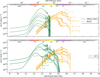 |
Fig. 1 Examples of the model templates included in AGNFITTER-RX for the physical components responsible for the emission of the host galaxy and its star-forming regions. At radio frequencies, the host-galaxy SED is dominated by the synchrotron emission associated with the diffusion of cosmic rays from SNR and PWN acceleration sites through the galaxy ISM, and the IR emission is dominated by the cold dust emission (green lines), both of which are associated with regions of high star-formation. The NIR–optical–UV emission is dominated by the stellar emission (yellow lines). The upper panel shows a subsample of semi-empirical templates by Chary & Elbaz (2001) and Dale & Helou (2002) for the emission from star-forming regions and the stellar population synthesis models by Bruzual & Charlot (2003) for SFH of 0.05 × 10⁹ yr, and different ages and metallicities. The lower panel shows theoretical models for cold dust by Schreiber et al. (2018) for increasing dust temperatures and fpah smoothly joined to the radio emission estimated with the FIR-radio correlation (Eq. (1)). |
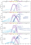 |
Fig. 2 Examples of the model templates included in AGNFITTER-RX for three distinct physical components of the nuclear emission (AGN) in active galaxies. At radio frequencies, the nuclear SED is dominated by the synchrotron emission (light blue curves) associated with jets and core emission at ~10−1−106 parsec scales. The MIR emission is dominated by the hot dusty “torus” emission (purple curves) arising at ~10 pc scales. The optical-UV-X-ray emission is dominated by the accretion disk and X-ray corona emission (dark blue curves) at ~10−2 pc scales. The first panel shows a SPL in radio, a subsample of torus templates by Silva et al. (2004) with different column densities, and the accretion disk model by Richards et al. (2006) with an increasing reddening parameter. The second panel presents SPL emission with different slopes, torus models by Nenkova et al. (2008) for different inclination angles and opening angles, and optical depth of 10, and accretion disk models by Slone & Netzer (2012) for diverse black holes masses and accretion rates. The third panel shows a DPL with curv and log νt as free parameters; torus templates by Stalevski et al. (2016) with optical depth of 3 and diverse inclination and opening angles; and accretion disk models by Kubota & Done (2018) defined by black holes masses and accretion rates. The fourth panel shows a DPL with log νt = 11.5 Hz and different values of α1 and α2; torus model by Hönig & Kishimoto (2017) depending on inclination angles, index of cloud distribution and cloud fractions; and the accretion disk template by Temple et al. (2021b). |
3.2 Infrared: Cold dust models
The emission of the cold dust from the star-forming regions in the host galaxy is modeled in AGNFITTER-RX using two optional sets of templates: a compilation of the semi-empirical libraries by Chary & Elbaz (2001) and Dale & Helou (2002) or the theoretical set of SEDs by Schreiber et al. (2018), hereafter denoted DH02_CE01 and S17, respectively.
DH02_CE01: A detailed description of DH02_CE01 library, which was included in the first version of the code, can be found in Calistro Rivera et al. (2016). The upper panel of Fig. 1 presents a subsample of SEDs of the library.
S17: The cold dust SED templates of Schreiber et al. (2018) consist of two independent components: the dust continuum and the mid-infrared emission line spectra from complex molecules. The first one is produced by big (>0.01 μm) and small (<0.01 μm) silicate and carbonate grains with “quasi-black body like” emissivity in the MIR-to-FIR range. The second component corresponds to the emission of lines between 3.3 and 12.3 μm due to the characteristic vibrational and rotational modes of polycyclic aromatic hydrocarbons (PAHs). Each component is modeled by 150 templates defined by two parameters: the dust temperature and the mass fraction of the PAH component (fPAH), which weights the contribution of PAHs to the total cold dust spectrum. The total spectrum is found by adding the SED of dust and PAHs for each possible combination of Tdust and fPAH, resulting in a flexible model consisting of 9600 templates. The flexibility of this model can be particularly useful to capitalize on new detailed observations of PAH emission in high-z galaxies and AGN with the James Webb Space Telescope (JWST). A subsample of templates is plotted in the lower panel of Fig. 1. For more details on this model, the reader may refer to Schreiber et al. (2018).
Thus, the number of free parameters is 2 (i.e., log IRlum and the normalization parameter SB) when choosing the DH02_CE01 model and 3 when choosing the S17 (i.e., Tdust, fracPAH and SB).
3.3 Infrared: AGN torus models
To model the emission from the nuclear hot dust and gas, commonly referred to as the AGN torus, we implement four different models: the semi-empirical model by Silva et al. (2004) and three theoretical models by Nenkova et al. (2008), Stalevski et al. (2016) and Hönig & Kishimoto (2017) hereafter S04, NK08, SKIRTOR and CAT3D-Wind, respectively. The theoretical models assume the existence of a population of (“clumpy”) dust clouds, resulting in lines of sight with probabilistic opacities that depend on the cloud spatial and density distribution.
S04: These semi-empirical templates consider the emission of a smooth distribution of dust. They were included in the first version of AGNFITTER (see Calistro Rivera et al. 2016 for a detailed description) and are presented in the upper panel of Fig. 2.
NK08: The CLUMPY model by Nenkova et al. (2008) considers dust clouds with a standard Galactic composition (53% silicates and 47% graphite) and column density of 1022−1023 cm−2 spread out in an axisymmetrical torus, internally limited by the dust sublimation region. The cloud distribution follows a Gaussian profile in the polar angle and a power law profile in the radial coordinate.
SKIRTOR: The two-phase model by Stalevski et al. (2016) consists of a torus composed of high-density clumps immersed in a smooth distribution of low-density dust. Templates were calculated with the continuum radiative transfer code SKIRT (Baes & Camps 2015; Camps & Baes 2015, 2020) by considering the geometry of a flared disk truncated the dust sublimation region. The dust distribution follows a power law profile with an exponential cut-off as a function of radius and polar angle, while the clumps scale radius of 0.4 pc and a density profile given by a standard smoothing kernel with compact support1, are generated randomly.
CAT3D: The CAT3D-Wind model (Hönig & Kishimoto 2017) considers dust and gas around AGNs as an ensemble of an inflowing clumpy disk and outflowing wind. Similar to NK08, the distribution of clouds with optical depth τν = 50 and radius of 0.035 times the graphite grains sublimation radius at 1500 K (rsub ~ 1 pc), is given radially by a power law but in the vertical direction follows a Gaussian distribution. A unique feature of this model is the inclusion of a polar wind component which is embedded in a hollow cone and, due to the sublimation in the innermost region of the torus, is only composed of big grains of dust.
In the last three cases, we include simplified versions of the models, since the original ones have 6, 6 and 8 fitting parameters, respectively. These large sets of SEDs are computationally demanding and may lead to overfitting of the data. Furthermore, in some cases, the spectral resolution of the SEDs may be insufficient to notice the effect of each parameter, which would cause the parameters to be unable to converge. For that reason, we reduced the number of templates by averaging all the models with respect to all but the 3 most relevant parameters (discussed through private communication with the authors of the models). We show in Sec. 6.1 that the reduction of the parameter space in these models is an approach to produce templates suitable for fitting. Those simplified templates deal with limitations relying on the existence, sensitivity, bandwidth, and spectral resolution of the rest-frame MIR data.
For NK08 and SKIRTOR are the inclination angle, opening angle and optical depth of the torus, while for CAT3D they are the inclination angle, index of the radial power law of the cloud distribution and fraction of clouds in the wind compared to the torus plane. As a result, our final SED grid consists of 1080, 400 and 378 templates for NK08, SKIRTOR and CAT3D, respectively, of which a subsample is plotted in the different panels of Fig. 2. As a consequence of the previous model reductions and considering the normalization parameter, a minimum of 2 (i.e., the normalization parameter TO and log NH or incl) and a maximum of 4 parameters (i.e., TO, incl, oa and τν or TO, incl, a and fwd, more details in Table 1) are required to model the torus emission.
AGNFITTER-RX fitting parameters.
3.4 Near-infrared/optical/UV: Stellar population models
The stellar emission templates were built employing the stellar population synthesis as in the first version of AGNFITTER. We took the single stellar population (SSP) models from Bruzual & Charlot (2003) defined for ages from 107 to 1010 yr and metallicities ranging from 0.004 to 0.04. This formalism includes a prescription for thermally pulsing stars in the asymptotic giant branch. To calculate the composite stellar population models we include the initial mass function by Chabrier (2003) and an exponentially decreasing star formation history (SFH). To account for a wider variety of stellar populations, 10 different characteristic times for the decay of SFH were considered with values between 0.05 to 11 Gyr. Unlike the first version of AGNFITTER, metallicity is now a free parameter of the SSPs. AGNFITTER-RX builds the stellar emission library using the SMPY code (Duncan & Conselice 2015), which gives the user the flexibility to include new templates with different star formation histories if desired. With new updates, the number of parameters required to fit the galaxy emission model is 4 or 5 (i.e., the normalization parameter GA, τ, age, Z, (B − V)gal) if we include metallicity.
3.5 Optical/UV: Accretion disk models
One of the main strengths of AGNFITTER in comparison to other SED-fitting codes is the superior modeling of the BH accretion disk emission and its reddening due to dust attenuation. AGNFITTER-RX further improves on this by including four libraries for the detailed modeling of the accretion disk emission2: a modified version of the semi-empirical templates by Richards et al. (2006) and Temple et al. (2021b) denoted as R06 and THB21, respectively; and the theory-built sets of templates by Slone & Netzer (2012) and Kubota & Done (2018), denoted as SN12 and KD18, respectively.
R06: The big blue bump model by Richards et al. (2006) is based on observed quasar spectra and a near-infrared (NIR) blackbody tail. The library is composed of one SED which is then modified by different levels of dust reddening following the Small Magellanic Cloud (SMC) dust attenuation law (upper panel of Fig. 2), and was implemented in the first version of the code (for more details see Calistro Rivera et al. 2016).
SN12: The emission model by Slone & Netzer (2012) is based on an α-disk model (optically thick and geometrically thin accretion disk), and the inclusion of relativistic temperature corrections, the effect of viscous dissipation and the comptonization of the radiation in the disk atmosphere. We include a simplified model by assuming a zero-spin black hole and windless disk, resulting in a set of 108 templates (some of them presented in the upper central panel of Fig. 2). The templates are parametrized by the mass of the SMBH taking values between of log MBH = [7.4, 9.8] in intervals of Δ log MBH = 0.3 and the accretion rate with values in the range
![Mathematical equation: $\[\dot{M} / \dot{M}_{\text {edd }}=[0.0,310.116]\]$](/articles/aa/full_html/2024/08/aa49329-24/aa49329-24-eq7.png) in variable intervals in the range
in variable intervals in the range ![Mathematical equation: $\[\Delta \dot{M} / \dot{M}_{\mathrm{edd}}=[0.001,154.69]\]$](/articles/aa/full_html/2024/08/aa49329-24/aa49329-24-eq8.png) .
.KD18: The theoretical model AGNSED (Kubota & Done 2018) considers the emission of an outer Novikov-Thorne accretion disk, an inner warm Comptonising region and a hot corona, all of them radially delimited. We adopted a simplified version which implied setting all the parameters except the black hole mass and the accretion rate to their typical values and assumed a second comptonisation component as a source of the soft X-ray excess (for more details see Kubota & Done 2018)3. The final set is composed of 225 SEDs defined by black hole masses between log MBH = [6, 10] in intervals of Δ log MBH = 0.286 and accretion rates in the range log
![Mathematical equation: $\[\dot{M} / \dot{M}_{\text {edd }}=[-1.5,0]\]$](/articles/aa/full_html/2024/08/aa49329-24/aa49329-24-eq9.png) in intervals of
in intervals of ![Mathematical equation: $\[\Delta \dot{M}=0.107\]$](/articles/aa/full_html/2024/08/aa49329-24/aa49329-24-eq10.png) . A subsample of the library is shown in the two lower panels of Fig. 2.
. A subsample of the library is shown in the two lower panels of Fig. 2.THB21: The accretion disk library by Temple et al. (2021b) is a set of composites empirically derived SED of luminous quasars. The templates include a broken power-law that models the accretion disk, a blackbody dominating from 1 to 3 μm due to hot dust; and account for both broad and narrow emission lines as well as additional continuum emission from blended line emission.
To soften the edges of the SED in AGNFITTER-RX, we add the low (ν < 1014.15 Hz) and high frequency (ν > 1015.5 Hz) tails of the R06 model by normalizing at the transition frequencies. The final template appertains to a zero redshift and nonreddened quasar with an average emission line template, and it is shown in the last panel of Fig. 2 after applying the AGNFITTER reddening prescription.
As mentioned in the R06 description, the different levels of extinction produced by dust are accounted for by applying the SMC reddening law (Prevot et al. 1984) to the nonreddened templates of all the aforementioned accretion disk models. The needed parameter in this prescription is the reddening E(B − V)BBB with values between 0 and 1. In summary, to fit the accretion disk component, the user needs between 2 (i.e., the normalization parameter BB and E(B − V)BBB) and 3 (i.e., log ![Mathematical equation: $\[M_{\mathrm{BH}}, \dot{M} / \dot{M}_{\mathrm{edd}}\]$](/articles/aa/full_html/2024/08/aa49329-24/aa49329-24-eq11.png) and E(B − V)BBB) parameters.
and E(B − V)BBB) parameters.
3.6 X-rays: Corona and star formation
For optical-UV accretion disk models which do not include X-rays, we add an X-ray model. Including the X-ray emission in AGN SED fitting is crucial as X-ray fluxes may be used to provide additional information to constrain accretion disk emission and break potential degeneracies between the blue accretion disk emission and galaxies with young/blue stellar populations in the optical-UV region. The X-ray emission is produced in the hot corona in the vicinity of the black hole, containing information related to the accretion process and the black hole properties. Considering the above, we used the empirical correlation αox − L2500Å (Lusso & Risaliti 2017; Just et al. 2007) which connects the coronae emission at 2 keV with the emission of the AGN at 2500 Å:
![Mathematical equation: $\[\alpha_{\mathrm{ox}}=-0.137 \log \left(L_{2500 Å}\right)+2.638 \text {, }\]$](/articles/aa/full_html/2024/08/aa49329-24/aa49329-24-eq12.png) (3)
(3)
where αox is the slope of the SED between 2500 Å and 2 keV given by:
![Mathematical equation: $\[\alpha_{\mathrm{ox}}=-0.3838 \log \left(L_{2500Å} / L_{2 \mathrm{keV}}\right).\]$](/articles/aa/full_html/2024/08/aa49329-24/aa49329-24-eq13.png) (4)
(4)
Based on the 2500 Å flux, we computed the expected αox from the relation. Then, we included a grid of dispersion values of Δαox, with respect to the empirical relation, to calculate the corresponding 2 keV fluxes for each accretion disk template. The dispersion of the relation is a fitting parameter taking a maximum value of Δαox = |0.4| reported by Lusso & Risaliti (2016) for low-quality data and sources with variability. Once the X-ray normalization is fixed, the SEDs were extended from 2 keV to more energetic X-rays by assuming a power law with a photon index of 1.8 and an exponential cut-off at 300 keV as assumed in Yang et al. (2020). When at least 2 X-ray measurements are available, the photon index is a free-fit parameter that takes values from 0.00 to 3.00 in intervals of ΔΓ = 0.15. We note that obscuration is not accounted for, and therefore this effective power law carries information about both obscuration and potential accretion rate estimates. Also, αox − L2500Å relation is valid to constrain soft X-ray emission only for type-1, radio-quiet, non-BAL4 AGNs (Strateva et al. 2005). Similarly, the SED of Blazars is likely modeled with synchrotron emission from radio to X-rays, and therefore αox − L2500Å relation is not providing reliable physical interpretation for those objects.
As part of the postprocessing analysis, we compute the host galaxy contribution to the X-rays due to the emission of high-mass X-ray binaries (HMXBs) and the hot ionized interstellar medium (ISM) using the formula provided by Mineo et al. (2014):
![Mathematical equation: $\[L_{0.5-8 \mathrm{keV}}=(4.0 \pm 0.4) \times 10^{39} \mathrm{SFR}\]$](/articles/aa/full_html/2024/08/aa49329-24/aa49329-24-eq14.png) (5)
(5)
where L0.5–8 keV is the luminosity between 0.5 and 8 keV in erg s−1 and SFR the star formation rate in M⊙yr−1. For this purpose, we used the IR SFR computed from the Murphy et al. (2011) calibration for the integrated 8–1000 μm luminosity of the cold dust emission:
![Mathematical equation: $\[\left(\frac{\mathrm{SFR}}{M_{\odot} \mathrm{yr}^{-1}}\right)=3.88 \times 10^{-44}\left(\frac{L_{\mathrm{IR}}}{\mathrm{erg} \mathrm{s}^{-1}}\right).\]$](/articles/aa/full_html/2024/08/aa49329-24/aa49329-24-eq15.png) (6)
(6)
Although we selected the most robust SFR estimator, it is worth noting that AGNFITTER-RX, as in its initial release, also delivers as output optical/UV SFR estimated from the stellar population emission (see Calistro Rivera et al. (2016) for more details). We included the host galaxy X-ray emission derived from the IR SFR in the estimation of the AGN fraction.
Table 1 presents a summary of the model-fitting parameters in AGNFITTER-RX, including names, values, and descriptions. The AGNFITTER code (Calistro Rivera et al. 2016), including the AGNFITTER-RX code release, are publicly available as open-source code in Python 3 in https://github.com/GabrielaCR/AGNfitter.
4 Data: Radio-to-X-ray SEDs of local AGN
To test the capabilities of AGNFITTER-RX, we fit the SEDs of a sample of 36 nearby active galaxies selected from the AGN SED ATLAS by Brown et al. (2019). This sample was chosen as it comprises a well-characterized and diverse set of local AGNs, with well-constrained photometric measurements with a high signal-to-noise ratio. To derive these synthetic SEDs, individual spectra were combined and scaled by a multiplicative factor to match aperture photometry measured from images using circular apertures. The scaling factors aim to relieve the effects of different instruments, extraction apertures and AGN variability producing discontinuities on the SEDs. The resulting photometric random uncertainties of the synthetic SEDs are extremely small compared to the errors in the photometric calibrations, scatter introduced by AGN variability and sources of systematic error since the AGNs in our sample are very bright. The photometric data is a compilation of available observations from GALEX, Swift, SDSS, PanSTARRS, Skymapper, 2MASS, WISE, Spitzer and Herschel, covering a broad wavelength range from the UV to the IR. For more details on the photometry, we refer the reader to Brown et al. (2019).
According to the spectroscopic classification by Véron-Cetty & Véron (2010), this sample includes eight Seyfert 1, five Seyfert 1n (Seyfert 1s with narrow Balmer lines), six Seyfert 1.2, eight Seyfert 1.5, one Seyfert 1.9, two Seyfert 2, one Seyfert 1i (Seyfert 2s with reddened broad line region), one LINER and four BL Lacertae objects.
To test the new AGNFITTER developments, we extended the spectral coverage of the Brown et al. (2019) SEDs by including archival photometric data in the radio and X-ray regimes. In the radio regime, we added 1.4, 5 and 15 GHz radio data from OVRO, Parkes, VLBA, VLA, Green Bank 140-ft, 100-m Effelsberg, 26-m Peach Mountain radio telescopes, obtained through the NASA/IPAC Extragalactic Database5. These bands were chosen because they were available for most AGNs (32 out of 36) in the sample.
In the X-rays, we added the 0.5–1 keV, 1–2 keV, 2–4.5 keV, and 4.5–12 keV bands from the XMM-Newton Serendipitous Source Catalogue 4XMM-DR11 (Webb et al. 2020). As explained by Yang et al. (2020), there are no standard transmission curves for X-ray bands due to the high sensibility of measurements to observing conditions and source characteristics. Hence, we follow the procedure by Risaliti & Lusso (2019) to calculate monochromatic fluxes at effective area-weighted mean energies (henceforth called pivot points) and include delta Dirac filters centered at those energies.
We got the pivot energies 0.76, 1.51, 3.22, and 6.87 keV for bands 2, 3, 4, and 5 of 4XMM-Newton, respectively, through private communication with the authors of the catalog. We computed correction factors (fcorr) to consider the effect of Galactic absorption while correcting for the difference between NH at the source location and the catalog assumed value. Factors were computed based on the reported and reference fluxes from Webb et al. (2020) for Γ = −1.42 and NH = 1.7 × 1020 cm−2, and the column densities from the gas map of the Python package gdpyc6. Thus, the corrected monochromatic fluxes at the pivot points were estimated as follows:
![Mathematical equation: $\[F_{\nu_2-\nu_1(\mathrm{corr})}=\nu^{(1+\Gamma)} \frac{F_{\nu_2-\nu_1}(2+\Gamma)}{\nu_2^{2+\Gamma}-\nu_1^{2+\Gamma}} f_{\text {corr }},\]$](/articles/aa/full_html/2024/08/aa49329-24/aa49329-24-eq16.png) (7)
(7)
where ![Mathematical equation: $\[F_{\nu_2-\nu_1}\]$](/articles/aa/full_html/2024/08/aa49329-24/aa49329-24-eq17.png) is the catalog reported flux within a given band, ν1 is lower and ν2 the upper-frequency limits of each band and a power law function with Γ = −1.42 (used to derive the fluxes in the 4XMM catalog) is assumed to model the X-ray emission. By definition, the monochromatic flux at the pivot energy does not depend on the photon index value assumed. The above procedure was possible for 29 of 36 AGNs in the sample with available X-ray data.
is the catalog reported flux within a given band, ν1 is lower and ν2 the upper-frequency limits of each band and a power law function with Γ = −1.42 (used to derive the fluxes in the 4XMM catalog) is assumed to model the X-ray emission. By definition, the monochromatic flux at the pivot energy does not depend on the photon index value assumed. The above procedure was possible for 29 of 36 AGNs in the sample with available X-ray data.
Our final data set comprises 36 galaxies, from which 25 have radio-to-X-ray coverage with up to 49 photometric data points, seven have radio-to-UV coverage with up to 45 photometric data points, and four have IR-to-X-ray coverage with up to 46 photometric data points. Of the 36 galaxies, 22 have FIR coverage. As photometry was not acquired at the same time, variability may be affecting our analysis. However, the trade-off is that we have very good wavelength coverage and high-quality photometry to perform the fittings. The extended photometric catalogs are published as supplementary data to this publication, and can be found in a Zenodo repository7.
5 Results
Figures 3 and 4 present examples of the fitting results that include Seyfert 1, Seyfert 1.5, Seyfert 2 AGN and blazars. The different curves represent the emission of the physical components corresponding to the most probable model (solid colour curves) and 10 realizations randomly selected from the posterior PDFs (shaded area). The line colors are coded similarly as in Figs. 1 and 2. The total SEDs are depicted as red lines and the observed photometry as black-filled circles with error bars. The lower part of each panel presents the residuals estimated as the difference between observed and model fluxes divided by the quadrature-combined errors of the photometry for each band. The residuals of the best model and ten random realizations are shown as red circles with outlined and shaded areas, respectively. The annotated maximum likelihood value is the highest value achieved by the live points in the nested sampling fitting process. The SED fitting plot of the remaining sources are also available as supplementary material in the Zenodo repository.
We employed the nested sampling method to perform the fits, which relies on a population of live points to explore parameter space. The iterative process removes the point with the lowest likelihood and searches for a new, independent point on ellipsoids around the remaining live points. The volume of live point decreases while the likelihood values increase. The process runs until the live point population is so small that does not contribute any probability mass.
This process takes approximately 25 min per source to fit a maximum of 19 parameters. We were able to concurrently run up to four sources, leveraging AGNFITTER-RX parallelization. While the computational time aligns with that of MCMC, the methods exhibit distinct convergence criteria. In emcee, convergence relies on assessing the effective number of independent samples within each chain, as measured by the integrated autocorrelation time. In contrast, UltraNest employs a convergence criterion based on the weight of the live points, since once this weight becomes negligible, it no longer improves the results, even if the iterations persist. The setup parameters were: 400 as the minimum number of live points, 400 effective samples, and 20 steps for the slice sampler.
It can be seen that different AGN classes require slightly different sets of models to optimize the fitting of the observed SED. This is not surprising as the AGNs in our sample are quite diverse. However, we can exploit the flexible capabilities of AGNFITTER-RX to investigate general trends of the different models included in the public version of the code and characterize how the results depend on the choice of the model. We also investigate the AGN physical components with the largest variety of models in the code, the torus and the accretion disk. For this purpose, we compare the performance of different models associated with a given component, while keeping fixed models for the other physical components. Isolating the effects of the different torus and disk models is of course complex due to dissimilar wavelength coverage and overlap with other physical components, such as stellar emission and cold dust, for instance.
For this purpose, we first set the R06 model for the disk, S17 for the cold dust, BC03 with metallicity for the stellar population and test the different hot dust models: 1 and 3 parameter versions of NK0, SKIRTOR, CAT3D; and the empirical S04. Once the best torus model was found, we proceeded to evaluate the different templates of the accretion disk using this model and maintaining S17 and B03 as cold dust and stellar population models. In all the runs, we assumed a flexible prior to constraining the cold dust to be at least as luminous as the dust-absorbed stellar emission.
The primary statistical outputs of the code are the distribution of logarithmic likelihood (log ![Mathematical equation: $\[\mathcal{L}\]$](/articles/aa/full_html/2024/08/aa49329-24/aa49329-24-eq18.png) ) for 100 random model realizations, its corresponding expected fluxes, the residuals compared to the data and the model logarithmic marginal likelihood (log Z from now on evidence). Beyond the quality of the fit informed by the likelihood and residuals, our Bayesian approach allows us to estimate and analyze posterior probabilities of the models given the observed SED P(MID). According to the Bayes theorem, it is define as:
) for 100 random model realizations, its corresponding expected fluxes, the residuals compared to the data and the model logarithmic marginal likelihood (log Z from now on evidence). Beyond the quality of the fit informed by the likelihood and residuals, our Bayesian approach allows us to estimate and analyze posterior probabilities of the models given the observed SED P(MID). According to the Bayes theorem, it is define as:
![Mathematical equation: $\[P(M \mid D)=\frac{P(D \mid M) P(M)}{P(D)}\]$](/articles/aa/full_html/2024/08/aa49329-24/aa49329-24-eq19.png) (8)
(8)
where P(D|M), P(D), and P(M) correspond to the likelihood, the evidence, and the prior probability of the models, respectively. As the sampling process outputs log ![Mathematical equation: $\[\mathcal{L}\]$](/articles/aa/full_html/2024/08/aa49329-24/aa49329-24-eq20.png) and log Z, we can compute log-posterior probabilities by assuming all the models are a priori equally probable. Due to the evidence term, posterior odds contain information of the probability of a given model to generate the observed SED by considering all combinations of parameters, enabling a robust model comparison.
and log Z, we can compute log-posterior probabilities by assuming all the models are a priori equally probable. Due to the evidence term, posterior odds contain information of the probability of a given model to generate the observed SED by considering all combinations of parameters, enabling a robust model comparison.
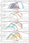 |
Fig. 3 Examples of the best SED fittings of the different AGN types: The blazar Mrk 421 is shown in the top panel, the Seyfert1 PG0052+251 in the second panel, the Seyfert 1.5 Mrk 290 in the third panel, and the Seyfert 2 Ark 564 in the bottom panel. The yellow and green solid curves show the emission from the stellar population and cold dust of the galaxy, respectively. Purple, dark blue, and light blue solid curves show the torus, accretion disk, and radio AGN emission models, respectively. Ten models constructed from combinations of parameters randomly selected from the posterior PDFs (hereafter referred to as realizations) are plotted as shaded areas and the residuals of each fit realization are presented in the graphs below each source. A flexible energy balance prior was assumed so that the cold dust IR emission is at least comparable to the dust-absorbed stellar emission. |
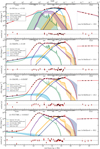 |
Fig. 4 Continued from Fig. 3. Examples of the best SED fittings for the blazar WCom, the Seyfert 1 Mrk876, and the Seyferts 1.5 Mrk509 and NGC7469. |
5.1 Comparing torus models
The first indicator that we use to compare the torus emission models is the likelihood, which is a measurement of the goodness of the fit. The likelihood distributions for 100 combinations of parameters randomly selected from the posterior PDFs (hereafter referred to as realizations) of the fits of the 36 galaxies in the sample are presented in the left panel of Fig. 5, for each of the torus models. We considered both relatively extended and simplified versions of the models, with 3 and 1 fitting parameters, respectively. Since the likelihood values are on a logarithmic scale, it implies all the histograms have a broad distribution. This feature is mainly due to the diversity in the AGN sample and highlights that some SEDs are better modeled than others.
The panels of Fig. 5 show how increasing model complexity may not necessarily imply a higher quality of the fit, given our current data. Although the NK08 and SKIRTOR models are driven by the same physical parameters and are equally simplified, NK08 has a very large increase in likelihood between the oneparameter and three-parameter models, reaching a difference of the order of ≈ 1040. In Appendix B.1 is presented the spectral slope space covered by our torus models given by α = − log(Fν(λ2)/Fν(λ1))/ log(λ2/λ1) with αMIR and αNIR corresponding to [λ2, λ1] equal to [14, 8] μm and [6, 3] μm; and the estimates of the rest-frame NIR and MIR spectral slope of our sample of AGNs based on Spitzer and WISE photometry. The plot shows how similar the areas covered by SKIRTOR with 3 and 1 parameters are in contrast to the different regions covered by NK08 with 3 and 1 parameters. This discrepancy in the αMIR-αNIR space might be responsible for the considerable likelihood increase from oneparameter to three-parameter templates. Additionally, NK08 oneparameter covers a lower range of $aLMIR compared to S04 and SKIRTOR oneparameter model, while most of the sources of our sample spread in wide range of low αMIR values which explains why the average NK08 is not performing so well. Consistently with the likelihood analysis, we found CAT3D and NK08 three-parameter are the closest models to the spectral slope space covered by our sample.
The histograms show that the more complex NK08 model results in the best overall distribution of fits, while the simplified version fails to capture important features of the SEDs. The set of templates in the simplified NK08 model does not exhibit the characteristic silicate 10 μm feature in absorption, only as an emission line, which changes its strength with the inclination angle of the torus. Meanwhile, the simplified version of the two-phase model SKIRTOR presents a transition between emission and absorption of the 10 μm line allowing to fit type 1, type 2 and intermediate AGNs such as those found in our sample. It raises the possibility of exploring another procedure for averaging NK08 SEDs in the future that yields a wide variety of silicate 10 μm features, likely the main driver of αMIR.
The inclusion of the polar wind component improves the quality of the fit, as can be seen in the central upper panel with the CAT3D model. The likelihood distribution is one of the narrowest and the one with the highest likelihood values. 25 out of 36 active galaxies achieved the maximum likelihood with CAT3D as the torus model in the fitting. These results suggest that using CAT3D with 3 parameters (i.e., incl, a, fwd) to model the torus gives the best result on average if we have a large enough number of photometric bands, and SKIRTOR with 1 parameter (i.e., incl) otherwise. Given that our sample comprises predominantly Sy1 AGNs (~83%) this finding is in agreement with that reported by García-Bernete et al. (2022); González-Martín et al. (2019) where the clumpy disk + wind model produces the best fit for Sy1. Favorable physical conditions and viewing angle of type 1 AGNs favor them for detecting IR dusty polar outflows. Similarly, recent SED studies of red quasars at intermediate redshifts (Calistro Rivera et al. 2021) suggest that the presence of dusty winds could potentially explain the IR excess at 2–5 μm in QSO SEDs. Specifically, the NIR bump can be explained by the presence of a hot graphite dust heated by the AGN (García-Bernete et al. 2017), reaching temperatures up to 1900 K and thus producing emission peaking in the NIR. However, alternative scenarios such as a contribution from direct emission from the accretion disk (Hernán-Caballero et al. 2016; González-Martín et al. 2019), host galaxy or a compact disk of host dust (Hönig et al. 2013; Tristram et al. 2014) have been proposed.
In the right panel of Fig. 5, we plot the combined residuals estimated as the difference between the observed data and the resulting models of SED fitting as a function of frequency for the complete sample. The purpose of this exercise is to search for general structure and trends for the different hot dust models which could inform us of their advantages and limitations in modeling specific frequencies of the IR regime. Around 10 μm (log νHz ~ 13.5), NK08 and CAT3D present negative residuals which means that most of the time, templates with emission features were fitted while the data suggest absorption features or no features, that is, the predicted fluxes are consistently overestimated by the models. This limitation may have effects on the uncertainties in the estimated inclination angle.
Moving towards shorter wavelengths, a positive bump is observed which implies an underestimation of fluxes between approximately 1.5 μm and 5 μm ![Mathematical equation: $\[\left(\log \frac{\nu}{\mathrm{~Hz}} \sim 14\right)\]$](/articles/aa/full_html/2024/08/aa49329-24/aa49329-24-eq21.png) . In S04 the bump has the highest amplitude meaning the highest overestimation, while in CAT3D and NK08 with 3 parameters the lowest ones. The behavior is consistent with the likelihood distributions and, due to the high amount of photometric bands that lie in this region, this bump largely determines the quality of the fit. This infrared excess, which is not recovered by models, has been reported previously in quasars and Seyfert galaxies (Mor et al. 2009; Burtscher et al. 2015; Temple et al. 2021a), and according to some studies it could be attributed to hot dusty winds not considered in most torus models (Calistro Rivera et al. 2021; Hönig 2019). This bump can potentially affect the properties of the host galaxies, making them brighter and redder than they would otherwise be.
. In S04 the bump has the highest amplitude meaning the highest overestimation, while in CAT3D and NK08 with 3 parameters the lowest ones. The behavior is consistent with the likelihood distributions and, due to the high amount of photometric bands that lie in this region, this bump largely determines the quality of the fit. This infrared excess, which is not recovered by models, has been reported previously in quasars and Seyfert galaxies (Mor et al. 2009; Burtscher et al. 2015; Temple et al. 2021a), and according to some studies it could be attributed to hot dusty winds not considered in most torus models (Calistro Rivera et al. 2021; Hönig 2019). This bump can potentially affect the properties of the host galaxies, making them brighter and redder than they would otherwise be.
Alternative analysis as the Akaike Information Criterion (AIC), founded on information theory, balances between fit quality and the complexity of the model by including an over-fitting penalisation term. AIC measures the loss of information in our understanding of the process that generates the data. The criteria are useful in the current comparison to assess if fitting simplified or complex torus models has a significant statistical effect. The model with the least loss of information, i.e., the lowest AIC, is favored. It is defined by the number of model parameters (k) and the maximum likelihood (![Mathematical equation: $\[\mathcal{L}\]$](/articles/aa/full_html/2024/08/aa49329-24/aa49329-24-eq22.png) ) as follows:
) as follows:
![Mathematical equation: $\[\mathrm{AIC}=-2 \ln \mathcal{L}-2 k.\]$](/articles/aa/full_html/2024/08/aa49329-24/aa49329-24-eq23.png) (9)
(9)
Table 2 presents the median of the distribution of maximum likelihoods for our sample of AGNs, its corresponding median logarithmic evidence, the median logarithmic posterior odds and the median AIC criteria. As observed in likelihood histograms of the realizations, the CAT3D model is the most favorable according to its high likelihood, high evidence and low AIC values. Since the evidence corresponds to a likelihood function integrated over all parameter space, it quantifies how well the high diversity of CAT3D templates in general explains the observed data. As the evidence increases, the posterior probability decreases, which means that, within the enormous possible combination of parameters, the specific producing the maximum likelihood is probably not the only one. The previous might be a consequence of potential model degeneracy which results in a slightly lower posterior probability (46.54%) for CAT3D compared to the highest (50.07%) value.
S04 presents the maximum mean posterior odds with ~4% higher probability than CAT3D, despite the lower likelihood values. Figure B.1 shows how the slope space covered by S04 is limited to a well-defined track, providing a limited variety of templates. Therefore, the S04 template producing the maximum likelihood, although it does not produce a high-quality fit, is the one that does the best within the set of possible S04 templates, meaning, its combination of parameters is the most likely.
In all the cases the Bayes factor Bij = Zi/Zj give a factor of more than 102 with strong evidence of the CAT3D model (log Zi = −80.83) concerning the other models (log Zj) according to the Jeffreys (1961) scale. For the oneparameter torus models the analysis is not conclusive since SKIRTOR presents a slightly higher likelihood and AIC, but lower evidence and posterior than S04. However, the Bayes factor BSKIRTOR,S04 = 10−0.11 ≈ 0.78 means a weak evidence supporting S04. Finally, it is worth highlighting that the increase in the parameter number in NK08 and SKIRTOR seems to have a subdominant effect on AIC compared to the likelihood improvement.
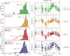 |
Fig. 5 Performance analysis of different torus models in SED fitting: The models presented are the homogeneous S04 (upper panel), the clumpy and windy CAT3D (central upper panel), the clumpy NK08 (central lower panel), and the two-phase SKIRTOR model (lower panel). The left panel shows the histograms of the logarithm of the likelihood values corresponding to each model and the dashed line in each plot indicates the median value of the distribution. Residuals from the best fits for each galaxy of the sample are shown in the right panel. The plot shows the existence of templates that manage to capture some SED features (high density of points around zero) while systematically failing in modeling specific regions of the observed SED (high dispersion). The dash-dotted line indicates the 10 μm feature and the dashed lines show the limits of 0σ, 3σ, and −3σ. |
Results of the torus model comparison.
5.2 Comparing accretion-disk models
Analogously to the previous comparison, we started by studying the likelihood distributions in the left panel of Fig. 6. In this case, the semi-empirical models R06 and THB21 reached higher likelihood values and narrower distributions than the theoretical models SN12 and KD18. THB21 produces the best fitting and is the unique model that considers emission lines in the spectrum. This result is informative since it shows that high-resolution spectral features of the broad AGN emission lines can have a high impact on the photometry (e.g., Schaerer & de Barros 2009; Shim et al. 2011; Marshall et al. 2022). In fact, the mean value of the likelihood distribution differs by a factor of ≈1010 from that of R06 even though both models were calibrated following a similar methodology with quasars and the redshift range of the data sets is the same. The limitation of these semi-empirical models, in comparison to the theoretical models discussed below, is that they do not provide any estimates of the physical properties of the black hole and accretion disk beyond SED luminosity or reddening.
Conversely, theoretical models have more difficulties in reproducing the shape of SEDs and this may be due to the limitations we still have to fully understand the emission of accretion disks. Despite the lower likelihood values, it would be interesting to study whether or not these models provide acceptable estimates, for example, of the black hole masses (see Sec. 6.2). In this way, we would be able to decipher in which cases it is convenient for the user to select one type of model or another given the scientific question they aim to answer.
In Appendix B.2 is presented the spectral slope space covered by our accretion disk models given by α = − log(Fν(λ2)/Fν(λ1))/ log(λ2/λ1) with and corresponding to [λ2, λ1] equal to [2500, 8.21] Å and [4420, 5400] Å; and the estimates of the rest-frame spectral slopes of our sample of AGNs based on GALEX, Swift and XMM-Newton photometry. The plot shows how the SN12 model using the flexible αox − L2500Å nicely overlaps our sources with both low αox and low αB-V while KD18 recovers some sources with αB-V. For our sample in particular, the parameter space covered by KD18 with BH mass and accretion rate as free parameters is not enough to mimic the spectral emission of some sources. Almost half of the sources outside the KD18 parameter space in Fig. B.2 account for the extended low probability tail of the probability distribution in Fig. 6. The lack of an X-ray obscuration prescription may be playing a role here, since absorption produces changes in the observed spectral slope, while the KD18 model only accounts for intrinsic photon index changes driven by the accretion rate.
The residuals in the right panel of Fig. 6 show a pronounced and narrow peak around λ ≈ 0.7 μm in all the models except THB21. This underestimation of the flux appears to be caused by the overlap of several emission lines such as the doublet of [N II] λλ6549, 6585 Å and H α λ 6563 Å, as suggested in previous works (e.g., Schaerer & de Barros 2009; Shim et al. 2011). In support of this, the errors in the THB21 model, which accounts for the emission lines, are very close to 0 and less dispersion of the points is observed, which is evidence of a systematic good fit. Besides, the FUV region contains a bump in all the models resulting from poor modeling of the soft excess as a consequence of the little good data in this region.
For a proper model comparison, we calculated the posterior odds (Eq. (8)) and the AIC criteria (Eq. (9)) as in the torus model comparison presented in the previous section. Table 3 summarizes the median distribution of maximum likelihoods for our sample of AGNs, its corresponding median logarithmic evidence, the median logarithmic posterior odds and the median AIC criteria. In this case, all the evaluated criteria agree with the likelihood distribution of the realizations (Fig. 6) in pointing to THB21 as the preferred accretion disk model. Despite R06 and THB21 being single templates without fitting parameters other than the normalization, reddening and the same X-ray αox recipe; the effect of the broad emission lines on the likelihood and evidence is significant. The Bayes factor of ≈105.1 also represents strong evidence of THB21 when compared with R06.
The theoretical SN12 model has similar results as R06 with just a smaller posterior but the Bayes factor 100.24 ≈ 1.74 suggests very strong evidence over R06. The AIC values show that for a similar fit quality, the increase of 1 fitting parameter of SN12 compared to R06 is not critical. Although the complexity of the KD18, both likelihood and evidence suggest templates are not diverse enough to produce high-quality fits, in particular at the X-rays regime. The inclusion of a third free parameter such as the spin, the spectral index of the warm Comptonisation component or the dissipated luminosity of the corona can improve the performance.
Results of the accretion disk model comparison.
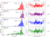 |
Fig. 6 Performance analysis of different accretion-disk models in SED fitting: The models shown are the semi-empirical R06 (upper panel), the semi-empirical with emission lines THB21 (central upper panel), the theoretical α-disk SN12 (central lower panel), and the theoretical three-component KD18 model (lower panel). The left panel shows the histograms of the logarithm of the likelihood values corresponding to each model and the dashed line in each plot indicates the median value of the distribution. Residuals from the best fits for each active galaxy of the sample are shown in the right panel. The effect of overlapped emission lines, such as the doublet of [N II] λλ 6549,6585 Å and H α λ 6563 Å, is large, reducing residuals to about zero. The dash-dotted line indicates the 0.65 μm broad emission lines feature and the dashed lines show the limits of 0σ, 3σ, and −3σ. |
5.3 Comparing model combinations
The best-fit results are produced using combinations of CAT3D and THB21 models for 67% of the sources. When analyzing type 1 and 2 AGNs independently, this success rate translates into 71% and 40%, respectively. However, there is not a sufficiently large sample of type 2 AGNs to obtain conclusive results. The 67% reaches a value of 81% when also considering combinations of CAT3D with other disk models such as R06, SN12 or KD18. The number of parameters required for these best fits is 19, consisting of five parameters associated with stellar models, three with cold-dust, four with the torus, two with accretion disk, two with X-rays and three with radio AGN models. This is not a problem for our data set as we have 49 photometric bands with a minimum of 40 valid data points, allowing convergence of the live points exploring the parameter space. However, if poorer sampling of the SEDs is available, then the simplified versions of the models might be required.
Current and upcoming surveys, such as JWST surveys and the Vera C. Rubin Observatory Legacy Survey of Space and Time (LSST), are poised to effectively sample the critical frequency ranges found in the residuals for the different emission models. The short and long wavelength channels of NIRCam on JWST are particularly well-suited for in-depth studies of the overlapping doublet of [N II] and H α emission lines in AGNs up to z ~ 6.5, as well as the torus NIR excess (3–4 μm restframe) in local AGNs. Additionally, MIRI imaging filters on JWST are sensitive to the crucial MIR torus peak and the silicate line in low-z AGNs, and they also capture the NIR excess in AGNs at wide redshift ranging up to z 6. The r, i, z, and y bands of LSST will enable the detection of the emission lines feature for AGNs at z < 0.5. These capabilities highlight the significant potential of current and near-future surveys to probe our torus and accretion disk models in the high redshift Universe.
When analyzing the morphology of the SEDs from Figs. 3 and 4 we can see how blazars present a highly decreasing spectrum in X-rays with Γ values around −2.69 and a high-energy emission of the accretion disk and the radio jet. Seyfert 1 AGNs present a high energy emission of the disk too but a lower energy radio emission and a less steep X-ray power law (Γ ≈ −2). On the contrary, in Seyfert 1.5 and 2 we observe a nuclear hot dust luminosity comparable to or slightly higher than that of the disk.
An important aspect we found evidence for, is how the X-ray fluxes help to break the degeneracy between the galaxy and AGN contribution to the UV, as can be seen for example in the SED fit of Ark 564. It can also be noted that despite the lack of information in the FIR in some cases such as Mrk 290 and Ark 564, it is possible to roughly estimate the emission of cold dust using the energy balance prior to the stellar emission.
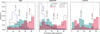 |
Fig. 7 Normalized histogram of the total distribution of inclination angle estimates by the NK08 (left panel), SKIRTOR (central panel) and CAT3D (right panel) model for the 36 galaxies of the sample classified as Seyfert 1 (light blue) and Seyfert 2 (magenta). The dotted contours represent the distribution of the angles for the oneparameter while the solid histograms for the three-parameter models. The solid vertical lines highlight the median values of the distributions. |
6 Discussion
The spectrum-like quality of this SED catalog results in extremely small photometric uncertainties as can be seen in Figs. 3 and 4. Despite point spread function and point source coincidence loss corrections were applied to observed photometry used to create the synthetic SEDs in Brown et al. (2019), no additional photometric calibration uncertainties were added to the final SEDs. A flux-to-error value matching the signal-to-noise ratio of the spectra, calibration uncertainties given by the instruments user handbook and/or fixed percentage errors can be incorporated to account for systematics in the models and instrumental effects (as in e.g., Leja et al. 2019 and Doore et al. 2021). Including the systematic effects can mitigate the significant under-fitting in some bands for even the best-fitting models. Furthermore, the much larger statistical weight of optical-radio data in the SEDs may dilute the contribution of the X-rays to the fit. To assess the potential consequences of the previous, we modified the X-ray uncertainties to equally weight the less energetic band by following the Zou et al. (2022) prescription and we performed again the SED fittings. Although the change in the likelihood values was expected due to its dependence on the photometric errors, no significant differences were found in the inferred physical parameters or the contribution of the AGN and host galaxy emission components. Then, the potential main drivers of the underfitting of our sample are systematic effects and AGN variability.
6.1 Current advances and limitations on the modeling of the torus
Previously, we discussed the clear bump we found in the residuals at 1.5–5 μm and how the CAT3D model reduces most of that feature, meaning that dusty winds might be a required element for ~70% of the sources. Beyond the quality of the fits achieved by the different models, we also wanted to evaluate the reliability and consistency of the inferred physical parameters.
As a first test, we compare the general trend of the inferred inclination angle parameter found by fitting different torus models to the SEDs of our sources with spectroscopic classifications (Véron-Cetty & Véron 2010). For simplicity, we group Blazars, Sy1, Sy1.2, Sy1.5 and Sy1n as Seyfert 1; and Sy1i, Sy2, Sy1.9 and Sy3 as Seyfert 2.
In Fig. 7 are shown the overall distributions of the inclination angle obtained for the 31 AGNs in our sample classified as Seyfert 1 and the five as Seyfert 2. For this, we evaluate the performance of the CAT3D models and the simplified and complex versions of NK08 and SKIRTOR. For all the three-parameter models, there is a difference of more than 22° in the median values of Sy1 and Sy2 distributions, which means that in principle we can use the inclination angle as a classifier of AGNs. As the distributions overlap, some Sy1 with large inclination angles and a few Sy2 with small angles, this classification would have to be done with caution. The Sy2 distributions for three-parameter models look quite wide probably due to the low number of AGNs. In particular, this distribution looks almost flat for the SKIRTOR model. Furthermore, it can be noted that SKIRTOR tends to find smaller angles for both Sy1 and Sy2 compared to the other models.
When using the oneparameter version of the NK08 and SKIRTOR models, the estimates of the inclination angle for Sy1 present narrower distributions centred at significantly smaller angles than the three-parameter models. This shows how the simplified version of SKIRTOR manages to find the most physically consistent angles for type 1 AGNs, perhaps by avoiding parameter degeneracies that may be occurring using the more complex version of this torus model. Instead, for the AGN type 2 population, the picture does not improve, as simplified versions of the models result in distribution histograms with very pronounced bimodalities with extreme peaks at around 10 and 80 degrees. Hence, the choice of the most suitable torus model to use depends on the properties of the AGNs as nuclear hydrogen column density, in accordance with what was reported in García-Bernete et al. (2022).
We then analyzed the self-consistency of models from a geometrical point of view, similar to a comparison done by Cerqueira-Campos et al. (2023). As proposed by the unified model (Antonucci & Miller 1985), the key spectral features of the diverse population of AGNs could be explained by the interaction of the light emitted by the active nuclei with the distribution of hot nuclear dust. Thus, the angle between the observer’s line of sight and the axis of the torus would determine the classification, being Type I and Type II AGNs the two endpoints of unobscured and highly obscured spectra. Comparing the inclination angle with the opening angle of the torus allows us to see whether indeed we reconstruct an edge-on or face-on orientation.
As shown in Fig. 8, the line of sights in Sy1 AGNs, estimated by the inclination angle parameter, are outside the toroidal distribution of hot dust for both the NK08 and SKIRTOR models. Even the 16th and 84th percentiles in the distribution of viewing angles do not intercept or have little overlap with dust distribution given by the torus opening angle. Conversely, Sy2 AGNs present distributions of the line of sight that completely intercept the torus for both models. It is outstanding how the SED fitting recovers torus aperture angles and uncertainties in the estimation of the observing angle that is consistently larger for Sy2 than for Sy1, which may be potentially associated with lower luminosity AGN (Wada 2012). SKIRTOR is more likely to result in smaller inclinations and larger aperture angles compared to NK08.
Another key physical feature which can be inferred from SED fitting is the estimation of the AGN contribution to the total luminosity in a certain energy range (AGN fraction), such as IR from 8 to 1000 μm or optical from 400 to 500 nm. In Fig. D.1 are presented the distributions of IR AGN fractions found by using each of the torus models in the fitting for each of the sources. With gray backgrounds, the galaxies lack SPIRE and PACS bands, crucial to constrain the emission of the galaxy starforming regions. It can be seen in Fig. D.1 how the uncertainties in the AGN fraction increase without FIR data. In these cases, AGNFITTER-RX can fit high and negligible contributions from cold dust affecting the estimation of the AGN fraction regardless of the choice of torus model. As a consequence, the violin plots of the mentioned galaxies are extended and are out of alignment, with different distributions of AGN fraction values. Since we used a flexible energy balance prior to running the fits, the attenuated stellar emission sets only a lower limit to the cold dust emission luminosity. Nevertheless, a more restrictive energy balance would have raised probabilities of models with a cold dust luminosity equal to the attenuated stellar component, largely constraining the IR AGN fraction and isolating the effect of the torus models. As previously stated, there are special cases in which the energy balance is broken so the decision of whether to include it or not, as well as the severity of the prior, is left to the user. For the active galaxies with available IR data, the change of hot dust model doesn’t affect the AGN IR luminosity.
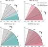 |
Fig. 8 Representation of the upper right quadrant of the cross-section of the toroidal distribution of hot nuclear dust in NK08 (upper panels) and SKIRTOR (lower panels) models. The shaded color areas with decreasing transparency represent the 16th, 50th and 84th percentiles of the torus opening angle in Seyfert 1 (blue) and Seyfert 2 (magenta) AGNs. While the black dotted lines represent the median values of the viewing angle and the dotted gray shaded areas are the 16th and 84th percentiles. |
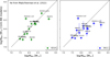 |
Fig. 9 Comparison of the log-scale black hole mass estimates made via AGNFITTER-RX using KD18 and SN12 accretion disk models (y-axis) and broad Hα emission line (x-axis) for 17 AGNs in our sample with available information in BASS DR2 catalog. The dotted line corresponds to the 1-to-1 relation. |
6.2 Current advances and limitations on accretion disk models
An important decision when choosing the accretion disk model for the SED fitting is whether to opt for semi-empirical or theoretical models. While the semi-empirical models have likelihood values potentially better than the latter (as THB21 in Fig. 6), theoretical models can provide estimates of important physical parameters such as the black hole mass and accretion rate. Using AGNFITTER-RX, black hole masses can be estimated from the rest-frame UV region of the observed SED only by applying SN12 or KD18 models. To evaluate the confidence of the values, in Fig. 9 we compare black hole masses from SED-fitting with virial estimates of black hole masses based on broad emission lines available for 17 AGNs from the BASS DR2 sample (Mejía-Restrepo et al. 2022). Since those spectroscopic estimates are reliable, we evaluate how the SED fitting estimates using KD18 (left) and SN12 (right) deviate from the one-to-one line.
It can be easily noticed how the KD18 model is in good agreement with the values of the BASS DR2 catalog. Out of the 13 sources, only three are outliers, while six are within the one-to-one ratio taking into account uncertainties and four others are off by only a factor of about 0.1 dex. These 13 sources are characterized by X-ray information, which is important for fitting the KD18 model extending up to hard X-rays (100 keV). However, as could be seen in Fig. 6, the likelihood histogram for the KD18 model has a peak around -log(like) ~ − 40 but a very spread out distribution reaching values of −200. A poor fit to stacked SEDs in the optical regime and unpredictable X-ray fluxes by up to a factor of 2 were also reported in Mitchell et al. (2023) for the log MBH regime between 7.5–9 M⊙. One possible explanation for this is that the continuum optical-to-X-rays templates require an observed SED in a narrow time window that ensures the variability is negligible compared to the photometric errors. As this is not guaranteed, sometimes the KD18 model fits well in the UV while producing high errors in the X-rays. Another alternative could be the X-ray obscuration producing changes in the observed spectral slope which does not correspond to the slope variations driven by the accretion rate in the KD18 templates. Precisely, AGNs with a correct estimate of the black hole mass are those that have a good X-ray fit with errors smaller than 2σ.
In the evaluation of the SN12 model, we included sources available in BASS DR2 even though their SEDs in our catalog did not have X-ray photometric bands, which increased our set from 13 to 17. The use of the αox relation combined with a power law with the dispersion of the relation (Δαox) and the photon index (Γ) as free parameters allow great flexibility in fitting X-rays. Therefore, X-ray photometry has a mild impact on the performance of specific accretion disk models. In this case, eight sources are clear outliers, six are successful estimates and three are off of the one-to-one relation by a factor of about 0.1 dex. The clustered sources around 108 M⊙ on the right side of the plot show how SN12 faces difficulties in estimating black hole masses for AGNs with masses greater than 108.5 M⊙.
It is worth noting that mass measurements from emission lines also have their assumptions and errors as the accretion disk emission models discussed above. The method assumed the dynamic of the gas in the broad line region is virialized, meaning the motion is produced by the gravitational field of the black hole. As mentioned in Mejía-Restrepo et al. (2022), the existence of winds can introduce biases by changing the observed gas dynamics. Additionally, the geometrical factor assumed to estimate the broad line region size in the empirical relations is a source of systematic errors. The specific value according to the chosen geometry or even the inclination angle, if a disk is assumed, increases the uncertainty.
Theoretical models yield estimates of the accretion rate as well, allowing the calculation of bolometric luminosities with the Eq. (C.1). In Fig. C.1, we contrast the bolometric luminosities computed via BH mass and accretion rate (BB model product) with the photometry value obtained by adding the integrated luminosities of the AGN-synchrotron, the torus, the accretion disk and the hot corona components (SED-fitting estimation). KD18 matches the AGN components estimates within the errors whereas SN12 systematically overestimates the bolometric luminosities by a factor 8. As our sources have BH masses dominantly in the range log MBH [M⊙] = 7.5–9, we are in the parameter space where KD18 templates have demonstrated to be successful in predicting BH mass and L2500 across different accretion rates (Mitchell et al. 2023). It can be noticed that: BBB models significantly reddened (EBVBBB > 0.6) resulting in larger bolometric luminosities than the SED-fitting estimations, in particular with the SN12 model; and the SED-fitting estimations are robust for both models despite of the individual normalization of the AGN components.
Finally, we again assess the effects of the different models, in this case of the accretion disk, on the estimates of the AGN fraction to the optical/UV emission. In Fig. D.2 are presented the distributions of optical AGN fractions (from 4000 to 5000 Å) found by using the R06, THB21, SN12 and KD18 models in the fitting. In most of the AGNs, the violin plots of all the models are aligned and even have a similar distribution width. However, within the observed outliers, the most frequent are distributions given by the theoretical models: SN12 and KD18. As shown in 2, opposite to the empirical models, the theoretical templates have a smooth shape in the big blue bump that hardly fits well the data in the most energetic region of the rest frame UV. The previous might be increasing the emission of the stellar population during the fits to reduce residuals and therefore, raising the contribution of the host galaxy. Also, the availability and shape of X-ray emission influence the fit quality due to the high and low flexibility of SN12 and KD18 while fitting X-rays, respectively. As discussed previously Fig. B.2 provides an indicator that the choice of free parameters in KD18 is not sufficient to produce diversity in the templates, especially in X-rays. Further research on the inclusion of relevant parameters such as spin, the spectral index of the warm Comptonisation component shaping the soft X-rays or the dissipated luminosity of the corona is needed. On the semi-empirical side, THB21 predicts a systematically larger host galaxy contribution to the SED of type 1 AGNs than R06.
6.3 The AGN contribution to the SED from the radio to X-rays
A key feature of SED fitting is the ability to disentangle the contributions of the AGN and the host galaxies to the overall emission. This contribution can significantly vary across wavelengths. Therefore, defining appropriate frequency regions where AGN fractions should be estimated is crucial. To provide information on this we use the flexibility of AGNFITTER-RX in delivering any customary range of AGN fraction provided by the user, and the unique coverage from the radio to the X-ray to compute a spectral AGN fraction distribution as presented in Fig. 10.
The AGN fraction within a frequency range is estimated as the ratio of the luminosity of the AGN model components, divided by the total observed luminosity (AGN + host galaxy), where the luminosities are estimated by integrating the model templates within the given frequency range. The frequency ranges used for the AGN fractions in Fig. 10 were chosen qualitatively, based on the photometric coverage in our data set. The width of the frequency ranges chosen in each case is represented by the maximal width of the violins. The violin plots in the upper and lower panel of Fig. 10 show the density distributions for the combined Sy1 or Sy2 populations, respectively, and illustrate a general trend of how the AGN contribution to the total emission changes as an function of frequency. The density distributions were obtained for each source by drawing 100 realizations from the posterior distributions of the Bayesian fit. In all cases, the long and thin tails in the distributions (e.g., the 4, 5, 7, 8, 9th violins from the left) are caused by a few outlier realizations from the posterior distributions that encountered models resulting in an AGN fraction distinct from that of the bulk of the realizations for a given source.
The blue and red curves represent the mean Sy1 and Sy2 SEDs, computed as the average best fit for each population, and are shown in the background for reference with an arbitrary normalization. The emission lines of the silicates and the broad line region can be clearly identified, as well as the big blue bump and a steep X-ray spectral slope characteristic of type 1 AGNs. IR-dominated dusty spectra with a mild UV nuclear emission, and a combination of steep and flat X-ray power laws characterize our average type 2 AGNs. Given the size of the Sy2 set, AGN fractions and the average SED might not be representative of the overall type 2 AGN population.
Both Sy1s and Sy2s exhibit dominant AGN emission in radio, MIR and X-ray bands, while emission in FIR bands appears galaxy-dominated. Indeed, this is in agreement with the most reliable methods for AGN selection, which rely on information from these energy ranges: IR-to-radio luminosity ratios (Condon et al. 1995), radio/FIR correlation (Helou et al. 1985; Donley et al. 2005), radio excess (Yun et al. 2001), radio power versus absolute K-band (infrared) magnitude (Hardcastle et al. 2019), MIR colors (Lacy et al. 2004; Stern et al. 2005; Donley et al. 2012), X-ray spectral slope (Alexander et al. 2005; Nandra & Pounds 1994), X-ray luminosities and X-ray to optical flux ratio (Szokoly et al. 2004; Lehmann et al. 2001), among others. By construction, optical-UV-based selection methods as UV excess are successful in unobscured AGNs (Boyle et al. 1990; Schmidt & Green 1983; Wisotzki et al. 1996; Verbeek et al. 2012), and incomplete for dust-obscured AGNs where the UV-optical is dominated by the host galaxy such as the type 2 ones. Consistently, only Sy1s in Fig. 10 have a high AGN fraction in UV bands.
Nonetheless, the extension and width of the violin plots evidence the diversity within the AGN populations and also, the degree of uncertainty in the estimate of the AGN fraction. In Sy1s the long and nearly equally wide violin in the FIR (3rd position from the left) is explained by the transition from AGN radio to galactic cold dust as the dominant emission component which occurs at different frequencies depending on the dust temperature and AGN properties. A similar phenomenon takes place at the transition from cold dust to torus (6th violin from the left), and from stellar to accretion disk emissions (4th and 5th violin from the right). In the Sy2s, though, the extended UV violin (2nd violin from the right) is a consequence of three of the five AGNs having so reddened accretion disk emission that stellar emission dominates, giving rise to a low AGN fraction, while the remaining sources the contributions are similar or dominated by the disk. We note that we used the observed accretion disk luminosities (the blue curve in Figs. 3, 4), not corrected for reddening, in our estimation of the AGN fraction. However, if we use the intrinsic (reddening-corrected) luminosity instead, the UV violin for the Sy2 population would be shifted towards higher values and a shape equivalent to the Sy1 population.
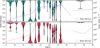 |
Fig. 10 AGN fraction distribution as a function of frequency for Sy1 (upper panel) and Sy2 (lower panel) populations. The white dots within the violin plots highlight the median of the distribution while the black line is the range between the 25th and 75th percentiles. The blue and red curves present the average radio-to-X-ray SED, including BC03_metal, S17, CAT3D, THB21, and combinations of SPL and DPL radio models, for type 1 and type 2 AGNs, respectively. |
7 Summary and conclusions
In this paper, we introduce the new radio-to-X-ray fitting capabilities of the Bayesian Python code AGNFITTER (Calistro Rivera et al. 2016), released as AGNFITTER-RX, which is designed to consistently fit the radio-to-X-ray SEDs of active galaxies by sampling the parameter space through MCMC or nested sampling. The physical model considers the contributions of the host galaxy, which consist of the emission from stellar populations, cold dust, and cosmic ray electrons in star-forming regions; as well as the AGN components, which include the emission of the hot corona, the accretion disk, the hot dust, and the radio emission from jets and/or shocks. The code now incorporates a variety of semi-empirical and theoretical emission models, as well as informative priors, including the assumption of the energy balance between dust-attenuated stellar emission and the re-emission by cold dust.
To test the new capabilities of the code, we used AGNFITTER-RX to fit 36 radio-to-X-ray SEDs of local active galaxies from the AGN SED ATLAS (Brown et al. 2019) at z < 0.7. In this study, we primarily selected this sample of well-characterized and diverse AGNs in order to assess and compare the performance of state-of-the-art torus and accretion disk emission models. We discuss the effects of different models on the fit quality and the most important infered physical properties. Once the best model combination was identifed and implemented, we also evaluate the performance of the code for different AGN populations.
- 1.
In ~70% of the studied sources, the inclusion of polar winds in torus models produced an advantage in the median of the likelihood distribution of more than three orders of magnitude, a Bayesian factor of higher than 100, and the lowest AIC values compared to other clumpy torus models. Considering that the sample is dominated by Sy1 AGNs, this result suggests that the presence of IR dusty polar outflows is essential in shaping the SEDs of type 1 AGNs.
- 2.
By comparing less complex torus template libraries, we find that the inclusion of absorption and emission silicate features likely plays a key role in achieving precise estimates of the inclination angles in most cases.
- 3.
We analyzed the fitted inclination angle (i.e., the line of sight) and the opening angle parameters of the hot nuclear dusty torus in the Type 1 and 2 AGNs. While the more complex torus models (more than three parameters) revealed overlapping broad inclination angle distributions, their simplified oneparameter versions yielded more physically consistent results with their spectroscopic classification, potentially alleviating parameter degeneracies inherent in complex torus models. However, the geometrical information obtained from the multiple parameters in the more complex torus models revealed lines of sight outside the toroidal hot dust distribution for Sy1 and lines of sight that fully intercept the torus for Sy2 AGNs, which are consistent with the AGN unification model.
- 4.
In ≈67% of cases, the accretion disk models that include emission lines stand out as the optimal choice for the fitting, with a likelihood distribution boasting a median value of >107 times higher, a Bayes factor of 105, and the lowest AIC values of all the model tested. Emission lines are crucial to avoiding the narrow peak in the residuals at 0.7 μm, which likely stems from the overlap of the doublet of [N II] λλ 6549,6585 Å and H α λ 6563 Å. While such empirical templates do not offer estimates for key properties such as black hole mass or accretion rate, this result underscores the substantial impact of high-resolution spectral features within broad AGN emission on the photometry, which agrees with previous studies.
- 5.
We conducted a comprehensive comparison between the black hole masses obtained from photometry only via SED fitting and virial estimates based on broad Hα emission lines. The theoretical model that incorporates X-ray emission demonstrates strong agreement with virial estimates, being consistent within the 0.1 dex range around the one-to-one ratio for ten out of 13 sources. Conversely, models that do not account for X-rays encounter difficulties in estimating black hole masses for AGNs exceeding 108.5 M⊙.
- 6.
We investigated the frequency dependence of estimated AGN fractions across the radio-to-Xray spectrum, finding that Sy1 and Sy2 exhibit dominant AGN emission in radio, MIR, and X-ray bands, in agreement with empirical AGN selection strategies. From our probabilistic analysis, we conclude that significant uncertainties in disentangling the AGN and galaxy emission in the IR and optical-UV can arise from the absence of FIR data, degeneracies between the accretion disk and host-galaxy UV emission, and the variable flexibility of models when fitting X-ray data.
The radio-to-X-ray SED fitting capabilities provided by AGNFITTER-RX are a powerful tool, allowing comprehensive studies of AGN physics. In addition to offering an unsurpassed wavelength coverage, AGNFITTER-RX allows the user to easily incorporate customary telescope filters, state-of-the-art theoretical and empirical model templates, and informative priors. AGNFITTER-RX is thus a promising and reliable tool for pushing boundaries at the interface between the observational and theoretical scientific communities, allowing them to test, compare, and customize models for the increasing data sets of deeper and larger panchromatic surveys.
In particular, AGNFITTER-RX was developed to capitalize on the present and future availability of exquisite radio and X-ray data sets, such as wide and deep radio surveys from the Low-Frequency Array (LOFAR; van Haarlem et al. 2013) and the Square Kilometre Array (SKA; McMullin et al. 2020), as well as new observational parameter spaces covered by X-ray observatories (e.g., eROSITA, Athena). Crucially, the focus of this investigation is the implementation and testing of IR AGN models of diverse complexity. While these complex models could only be explored in the nearby Universe until recently, the remarkable sensitivity, resolution, and wavelength coverage provided by the JWST will now allow us to test and use these models at intermediate and high redshifts. The rich library of IR AGN and host-galaxy models in AGNFITTER-RX is therefore ideal for modeling JWST/MIRI, JWST/NIRCam, HST, and Euclid photometry in order to investigate the hot dust emission, physics, and geometry of AGN obscuration at high-z, including polar dust distributions, and the disentanglement of AGN emission from star formation.
The AGNFITTER code (Calistro Rivera et al. 2016), including the AGNFITTER-RX code release, are publicly available as open-source Python 3 code at GitHub8.
Acknowledgements
We gratefully acknowledge support from the National Agency for Research and Development (ANID) under the fellowship ANID Becas/Doctorado Nacional, #21220337 (LNMR-R), Millennium Science Initiative Program – ICN12_009 (LNM-R, FEB), CATA-BASAL – FB210003 (LNM-R, FEB), and FONDECYT Regular – #1200495 (LNM-R, FEB); the Vicerrectoría de Investigación of Pontificia Universidad Católica de Chile under the fellowship Stay of Doctoral Co-tutelage Abroad, leading to double degree; the Vicerrectoría de Investigación y Extensión de la Universidad Industrial de Santander under project 2494 (JCBP); and the Ministry of Science, Technological Development and Innovation of the Republic of Serbia, through contract No. 451-03-9/2024-14/200002 (MS). We thank Sebastian Höning, Paolo Padovani and Christine Done for useful comments, valuable discussions and suggestions on the implementation of CAT3D-WIND, KD18 and synchrotron emission models. We thank David W Hogg and Luis A. Núñez for their support during the initial phases of the project.
Appendix A Catalog of fitted AGNs
Sample of 36 local AGNs from SED ATLAS.
Appendix B Parameter space covered by the models
Spectral slope space covered by the torus models included in this study, given by α = − log(Fν(λ2)/Fν(λ1))/ log(λ2/λ1) with αMIR and αNIR corresponding to [λ2, λ1] equal to [14, 8] and [6, 3] μm. The estimates for the AGNs of our sample were based on WISE band 3 at λ = 12 μm and IRAC band 4 at λ = 8 μm for αMIR; and IRAC band 3 at λ = 5.8 μm and WISE band 1 at λ = 3.4 μm for αNIR.
Similarly, the spectral slope space covered by the accretion disk models was computed with αb-v and αox corresponding to [λ2, λ1] equal to [4420, 5400] and [2500, 8.21] Å. The slopes of our sample were based on Swift band B at λ = 4392 Å and Swift band V at λ = 5468 Å for αnir, and GALEX NUV channel at λ = 2500 Å and XMM-Newton band 3 for αox.
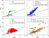 |
Fig. B.1 αMIR-αNIR spectral slope space covered by the different torus models included in AGNFITTER-RX with different complexity levels. The gray circles show estimates of the spectral slope covered by our sample of AGN, computed with Spitzer and WISE observed photometry. |
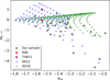 |
Fig. B.2 αox-αB-V spectral slope space covered by the different accretion disk models included in AGNFITTER-RX. The gray circles show estimates of the spectral slope covered by our sample of AGN, computed with Swift, GALEX and XMM-Newton observed photometry. |
Appendix C Bolometric luminosity from accretion disk models
We compute bolometric luminosities based on the black hole mass and accretion rate estimates from the theoretical accretion disk models SN12 and KD18 as follows:
![Mathematical equation: $\[L_{\mathrm{bol}}=\left(\frac{\dot{m}}{\dot{m}_{\mathrm{edd}}}\right) \times 1.26 \times 10^{38} \times M_{\mathrm{BH}}\]$](/articles/aa/full_html/2024/08/aa49329-24/aa49329-24-eq26.png) (C.1)
(C.1)
and compare with the values obtained by adding the integrated luminosities of the AGN-synchrotron, the torus, the accretion disk and the hot corona components.
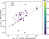 |
Fig. C.1 Bolometric luminosities are computed by adding integrated luminosities of the AGN components vs bolometric luminosities based on the inferred black hole mass and accretion rate by the accretion disk models. The gray dashed line indicates the one-to-one ratio and the color bar is the accretion disk reddening parameter. |
Appendix D IR and optical AGN fraction
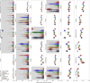 |
Fig. D.1 AGN fraction contributing to the total IR luminosity (8 − 1000 μm) for the 36 galaxies of the sample and each torus model tested. The gray area highlights the SEDs with missing data in the FIR. The different models used do not have a large effect on the overall AGN fraction in this range. |
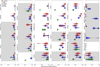 |
Fig. D.2 AGN fraction contributing to the total optical luminosity (400 − 500nm) for the 36 galaxies of the sample and each accretion disk model tested. The flexibility in modeling X-rays and the effects of UV degeneracy causes outliers more often with the KD18 accretion disk model. |
References
- Ackermann, M., Ajello, M., Allafort, A., et al. 2011, ApJ, 741, 30 [NASA ADS] [CrossRef] [Google Scholar]
- Aghanim, N., Akrami, Y., Ashdown, M., et al. 2020, A&A, 641, A6 [NASA ADS] [CrossRef] [EDP Sciences] [Google Scholar]
- Alexander, D., Bauer, F., Chapman, S., et al. 2005, ApJ, 632, 736 [NASA ADS] [CrossRef] [Google Scholar]
- Antonucci, R., & Miller, J. 1985, ApJ, 297, 621 [NASA ADS] [CrossRef] [Google Scholar]
- Asmus, D., Hoenig, S. F., & Gandhi, P. 2016, ApJ, 822, 109 [NASA ADS] [CrossRef] [Google Scholar]
- Azadi, M., Wilkes, B., Kuraszkiewicz, J., et al. 2023, ApJ, 945, 145 [NASA ADS] [CrossRef] [Google Scholar]
- Baan, W., & Klöckner, H.-R. 2006, A&A, 449, 559 [NASA ADS] [CrossRef] [EDP Sciences] [Google Scholar]
- Baes, M., & Camps, P. 2015, Astron. Comput., 12, 33 [NASA ADS] [CrossRef] [Google Scholar]
- Bell, E. F. 2003, ApJ, 586, 794 [Google Scholar]
- Berta, S., Lutz, D., Santini, P., et al. 2013, A&A, 551, A100 [NASA ADS] [CrossRef] [EDP Sciences] [Google Scholar]
- Blandford, R., Netzer, H., Woltjer, L., Courvoisier, T.-L., & Mayor, M. 1990, Active Galactic Nuclei, 97 [Google Scholar]
- Boyle, B., Fong, R., Shanks, T., & Peterson, B. 1990, MNRAS, 243, 1 [NASA ADS] [Google Scholar]
- Brown, M. J. I., Duncan, K. J., Landt, H., et al. 2019, MNRAS, 489, 3351 [Google Scholar]
- Bruzual, G., & Charlot, S. 2003, MNRAS, 344, 1000 [NASA ADS] [CrossRef] [Google Scholar]
- Buat, V., Ciesla, L., Boquien, M., Małek, K., & Burgarella, D. 2019, A&A, 632, A79 [NASA ADS] [CrossRef] [EDP Sciences] [Google Scholar]
- Buchner, J. 2014, Statist. Comput., 26, 383 [Google Scholar]
- Buchner, J. 2019, PASP, 131, 108005 [Google Scholar]
- Burtscher, L., de Xivry, G. O., Davies, R., et al. 2015, A&A, 578, A47 [NASA ADS] [CrossRef] [EDP Sciences] [Google Scholar]
- Calistro Rivera, G., Lusso, E., Hennawi, J. F., & Hogg, D. W. 2016, ApJ, 833, 98 [Google Scholar]
- Calistro Rivera, G., Williams, W., Hardcastle, M., et al. 2017, MNRAS, 469, 3468 [NASA ADS] [CrossRef] [Google Scholar]
- Calistro Rivera, G., Hodge, J. A., Smail, I., et al. 2018, ApJ, 863, 56 [Google Scholar]
- Calistro Rivera, G., Alexander, D., Rosario, D., et al. 2021, A&A, 649, A102 [NASA ADS] [CrossRef] [EDP Sciences] [Google Scholar]
- Calistro Rivera, G., Alexander, D. M., Harrison, C. M., et al. 2023, A&A submitted, [arXiv:2312.10177] [NASA ADS] [CrossRef] [EDP Sciences] [Google Scholar]
- Camps, P., & Baes, M. 2015, Astron. Comput., 9, 20 [Google Scholar]
- Camps, P., & Baes, M. 2020, Astron. Comput., 31, 100381 [NASA ADS] [CrossRef] [Google Scholar]
- Cerqueira-Campos, F., Rodríguez-Ardila, A., Panda, S., et al. 2023, MNRAS, 524, 542 [NASA ADS] [CrossRef] [Google Scholar]
- Chabrier, G. 2003, PASP, 115, 763 [Google Scholar]
- Chary, R., & Elbaz, D. 2001, ApJ, 556, 562 [Google Scholar]
- Ciesla, L., Charmandaris, V., Georgakakis, A., et al. 2015, A&A, 576, A10 [NASA ADS] [CrossRef] [EDP Sciences] [Google Scholar]
- Comastri, A. 2004, Supermassive Black Holes in the Distant Universe, 245 [NASA ADS] [CrossRef] [Google Scholar]
- Condon, J. J. 1992, ARA&A, 30, 575 [Google Scholar]
- Condon, J., Anderson, E., & Broderick, J. 1995, AJ, 109, 2318 [NASA ADS] [CrossRef] [Google Scholar]
- Da Cunha, E., Charlot, S., & Elbaz, D. 2008, MNRAS, 388, 1595 [NASA ADS] [CrossRef] [Google Scholar]
- Dale, D. A., & Helou, G. 2002, ApJ, 576, 159 [Google Scholar]
- Davis, S. W., Woo, J.-H., & Blaes, O. M. 2007, ApJ, 668, 682 [NASA ADS] [CrossRef] [Google Scholar]
- De Jong, T., Klein, U., Wielebinski, R., & Wunderlich, E. 1985, A&A, 147, L6 [Google Scholar]
- Delvecchio, I., Daddi, E., Sargent, M., et al. 2021, A&A, 647, A123 [NASA ADS] [CrossRef] [EDP Sciences] [Google Scholar]
- Donley, J., Rieke, G., Rigby, J., & Pérez-González, P. 2005, ApJ, 634, 169 [NASA ADS] [CrossRef] [Google Scholar]
- Donley, J. L., Koekemoer, A. M., Brusa, M., et al. 2012, ApJ, 748, 142 [Google Scholar]
- Doore, K., Eufrasio, R. T., Lehmer, B. D., et al. 2021, ApJ, 923, 26 [NASA ADS] [CrossRef] [Google Scholar]
- Duncan, K., & Conselice, C. J. 2015, MNRAS, 451, 2030 [NASA ADS] [CrossRef] [Google Scholar]
- Esparza-Arredondo, D., Gonzalez-Martín, O., Dultzin, D., et al. 2021, A&A, 651, A91 [NASA ADS] [CrossRef] [EDP Sciences] [Google Scholar]
- Foreman-Mackey, D., Hogg, D. W., Lang, D., & Goodman, J. 2013, PASP, 125, 306 [Google Scholar]
- García-Bernete, I., Ramos Almeida, C., Landt, H., et al. 2017, MNRAS, 469, 110 [CrossRef] [Google Scholar]
- García-Bernete, I., González-Martín, O., Almeida, C. R., et al. 2022, A&A, 667, A140 [NASA ADS] [CrossRef] [EDP Sciences] [Google Scholar]
- González-Martín, O., Masegosa, J., García-Bernete, I., et al. 2019, ApJ, 884, 11 [Google Scholar]
- Hardcastle, M., Williams, W., Best, P., et al. 2019, A&A, 622, A12 [NASA ADS] [CrossRef] [EDP Sciences] [Google Scholar]
- Helou, G., Soifer, B., & Rowan-Robinson, M. 1985, ApJ, 298, L7 [NASA ADS] [CrossRef] [Google Scholar]
- Hernán-Caballero, A., Hatziminaoglou, E., Alonso-Herrero, A., & Mateos, S. 2016, MNRAS, 463, 2064 [Google Scholar]
- Hönig, S. F. 2019, ApJ, 884, 171 [Google Scholar]
- Hönig, S. F., & Kishimoto, M. 2017, ApJ, 838, L20 [Google Scholar]
- Hönig, S. F., Kishimoto, M., Tristram, K. R., et al. 2013, ApJ, 771, 87 [CrossRef] [Google Scholar]
- Jeffreys, H. 1961, International series of monographs on physics (Oxford University Press) [Google Scholar]
- Just, D. W., Brandt, W. N., Shemmer, O., et al. 2007, ApJ, 665, 1004 [Google Scholar]
- Kang, J.-L., & Wang, J.-X. 2022, ApJ, 929, 141 [NASA ADS] [CrossRef] [Google Scholar]
- Kubota, A., & Done, C. 2018, MNRAS, 480, 1247 [Google Scholar]
- Lacy, M., Storrie-Lombardi, L. J., Sajina, A., et al. 2004, ApJS, 154, 166 [Google Scholar]
- Lehmann, I., Hasinger, G., Schmidt, M., et al. 2001, A&A, 371, 833 [NASA ADS] [CrossRef] [EDP Sciences] [Google Scholar]
- Leja, J., Johnson, B. D., Conroy, C., & Van Dokkum, P. 2018, ApJ, 854, 62 [NASA ADS] [CrossRef] [Google Scholar]
- Leja, J., Carnall, A. C., Johnson, B. D., Conroy, C., & Speagle, J. S. 2019, ApJ, 876, 3 [Google Scholar]
- Lusso, E., & Risaliti, G. 2016, ApJ, 819, 154 [Google Scholar]
- Lusso, E., & Risaliti, G. 2017, A&A, 602, A79 [NASA ADS] [CrossRef] [EDP Sciences] [Google Scholar]
- Marshall, A., Auger-Williams, M. W., Banerji, M., Maiolino, R., & Bowler, R. 2022, MNRAS, 515, 5617 [CrossRef] [Google Scholar]
- Matt, G., Guainazzi, M., & Maiolino, R. 2003, MNRAS, 342, 422 [NASA ADS] [CrossRef] [Google Scholar]
- McMullin, J., Diamond, P., McPherson, A., et al. 2020, in Ground-based and Airborne Telescopes VIII, 11445, SPIE, 215 [Google Scholar]
- Mejía-Restrepo, J. E., Trakhtenbrot, B., Koss, M. J., et al. 2022, ApJS, 261, 5 [CrossRef] [Google Scholar]
- Mineo, S., Gilfanov, M., Lehmer, B., Morrison, G., & Sunyaev, R. 2014, MNRAS, 437, 1698 [NASA ADS] [CrossRef] [Google Scholar]
- Mitchell, J. A., Done, C., Ward, M. J., et al. 2023, MNRAS, 524, 1796 [NASA ADS] [CrossRef] [Google Scholar]
- Molnár, D. C., Sargent, M. T., Leslie, S., et al. 2021, MNRAS, 504, 118 [CrossRef] [Google Scholar]
- Mor, R., Netzer, H., & Elitzur, M. 2009, ApJ, 705, 298 [Google Scholar]
- Murphy, E., Condon, J., Schinnerer, E., et al. 2011, ApJ, 737, 67 [NASA ADS] [CrossRef] [Google Scholar]
- Nandra, K., & Pounds, K. 1994, MNRAS, 268, 405 [NASA ADS] [CrossRef] [Google Scholar]
- Nardini, E., Reeves, J., Gofford, J., et al. 2015, Science, 347, 860 [NASA ADS] [CrossRef] [Google Scholar]
- Nenkova, M., Sirocky, M. M., Nikutta, R., Ivezić, Ž., & Elitzur, M. 2008, ApJ, 685, 160 [Google Scholar]
- Netzer, H. 2015, ARA&A, 53, 365 [Google Scholar]
- Padovani, P., Alexander, D., Assef, R., et al. 2017, A&ARv, 25, 1 [NASA ADS] [CrossRef] [Google Scholar]
- Panessa, F., Baldi, R. D., Laor, A., et al. 2019, Nat. Astron., 3, 387 [Google Scholar]
- Peterson, B. M. 1993, PASP, 105, 247 [NASA ADS] [CrossRef] [Google Scholar]
- Polletta, M., Courvoisier, T.-L., Hooper, E., et al., 2000, A&A, 362, 75 [NASA ADS] [Google Scholar]
- Prevot, M., Lequeux, J., Maurice, E., Prévot, L., & Rocca-Volmerange, B. 1984, A&A, 132, 389 [Google Scholar]
- Richards, G. T., Strauss, M. A., Fan, X., et al. 2006, AJ, 131, 2766 [Google Scholar]
- Risaliti, G., & Lusso, E. 2019, Nat. Astron., 3, 272 [Google Scholar]
- Schaerer, D., & de Barros, S. 2009, A&A, 502, 423 [NASA ADS] [CrossRef] [EDP Sciences] [Google Scholar]
- Schmidt, M., & Green, R. F. 1983, ApJ, 269, 352 [NASA ADS] [CrossRef] [Google Scholar]
- Schreiber, C., Elbaz, D., Pannella, M., et al. 2018, A&A, 609, A30 [NASA ADS] [CrossRef] [EDP Sciences] [Google Scholar]
- Shim, H., Chary, R.-R., Dickinson, M., et al. 2011, ApJ, 738, 69 [NASA ADS] [CrossRef] [Google Scholar]
- Silpa, S., Kharb, P., Harrison, C., et al. 2022, MNRAS, 513, 4208 [NASA ADS] [CrossRef] [Google Scholar]
- Silva, L., Maiolino, R., & Granato, G. L. 2004, MNRAS, 355, 973 [Google Scholar]
- Slone, O., & Netzer, H. 2012, MNRAS, 426, 656 [NASA ADS] [CrossRef] [Google Scholar]
- Smith, D., Jarvis, M., Hardcastle, M., et al. 2014, MNRAS, 445, 2232 [NASA ADS] [CrossRef] [Google Scholar]
- Stalevski, M., Ricci, C., Ueda, Y., et al. 2016, MNRAS 458, 2288 [Google Scholar]
- Stalevski, M., Tristram, K. R., & Asmus, D. 2019, MNRAS, 484, 3334 [NASA ADS] [CrossRef] [Google Scholar]
- Stern, D., Eisenhardt, P., Gorjian, V., et al. 2005, ApJ, 631, 163 [Google Scholar]
- Strateva, I. V., Brandt, W., Schneider, D. P., Berk, D. G. V., & Vignali, C. 2005, AJ, 130, 387 [NASA ADS] [CrossRef] [Google Scholar]
- Szokoly, G. P., Bergeron, J., Hasinger, G., et al. 2004, ApJS, 155, 271 [NASA ADS] [CrossRef] [Google Scholar]
- Tanimoto, A., Ueda, Y., Odaka, H., et al. 2019, ApJ, 877, 95 [Google Scholar]
- Temple, M. J., Banerji, M., Hewett, P. C., Rankine, A. L., & Richards, G. T. 2021a, MNRAS, 501, 3061 [Google Scholar]
- Temple, M. J., Hewett, P. C., & Banerji, M. 2021b, MNRAS, 508, 737 [NASA ADS] [CrossRef] [Google Scholar]
- Thorne, J. E., Robotham, A. S. G., Davies, L. J. M., et al. 2022, MNRAS, 509, 4940 [Google Scholar]
- Tombesi, F., Meléndez, M., Veilleux, S., et al. 2015, Nature, 519, 436 [NASA ADS] [CrossRef] [Google Scholar]
- Tristram, K. R., Burtscher, L., Jaffe, W., et al. 2014, A&A, 563, A82 [CrossRef] [EDP Sciences] [Google Scholar]
- Urry, C. M., & Padovani, P. 1995, PASP, 107, 803 [NASA ADS] [CrossRef] [Google Scholar]
- van Haarlem, M. P., Wise, M. W., Gunst, A., et al. 2013, A&A, 556, A2 [NASA ADS] [CrossRef] [EDP Sciences] [Google Scholar]
- Verbeek, K., de Groot, E., Groot, P. J., et al. 2012, MNRAS, 420, 1115 [NASA ADS] [CrossRef] [Google Scholar]
- Véron-Cetty, M.-P., & Véron, P. 2010, A&A, 518, A10 [NASA ADS] [CrossRef] [EDP Sciences] [Google Scholar]
- Wada, K. 2012, ApJ, 758, 66 [Google Scholar]
- Webb, N., Coriat, M., Traulsen, I., et al. 2020, A&A, 641, A136 [NASA ADS] [CrossRef] [EDP Sciences] [Google Scholar]
- Wisotzki, L., Köhler, T., Groote, D., & Reimers, D. 1996, A&AS, 115, 227 [NASA ADS] [Google Scholar]
- Yang, G., Boquien, M., Buat, V., et al. 2020, MNRAS, 491, 740 [Google Scholar]
- Yun, M. S., Reddy, N. A., & Condon, J. 2001, ApJ, 554, 803 [NASA ADS] [CrossRef] [Google Scholar]
- Zou, F., Brandt, W., Chen, C.-T., et al. 2022, ApJS, 262, 15 [NASA ADS] [CrossRef] [Google Scholar]
See https://www.particleworks.com/technical_column_vol3_02_en.html for brief explanation.
We use “accretion disk emission” to refer to the UV and optical emission from the region inside the dust sublimation radius, including the broad line region.
The Python code to generate the templates can be found at https://github.com/arnauqb/qsosed
BAL: Broad absorption line.
Gas and Dust Python Calculator.
All Tables
All Figures
|
Fig. 1 Examples of the model templates included in AGNFITTER-RX for the physical components responsible for the emission of the host galaxy and its star-forming regions. At radio frequencies, the host-galaxy SED is dominated by the synchrotron emission associated with the diffusion of cosmic rays from SNR and PWN acceleration sites through the galaxy ISM, and the IR emission is dominated by the cold dust emission (green lines), both of which are associated with regions of high star-formation. The NIR–optical–UV emission is dominated by the stellar emission (yellow lines). The upper panel shows a subsample of semi-empirical templates by Chary & Elbaz (2001) and Dale & Helou (2002) for the emission from star-forming regions and the stellar population synthesis models by Bruzual & Charlot (2003) for SFH of 0.05 × 10⁹ yr, and different ages and metallicities. The lower panel shows theoretical models for cold dust by Schreiber et al. (2018) for increasing dust temperatures and fpah smoothly joined to the radio emission estimated with the FIR-radio correlation (Eq. (1)). |
| In the text | |
|
Fig. 2 Examples of the model templates included in AGNFITTER-RX for three distinct physical components of the nuclear emission (AGN) in active galaxies. At radio frequencies, the nuclear SED is dominated by the synchrotron emission (light blue curves) associated with jets and core emission at ~10−1−106 parsec scales. The MIR emission is dominated by the hot dusty “torus” emission (purple curves) arising at ~10 pc scales. The optical-UV-X-ray emission is dominated by the accretion disk and X-ray corona emission (dark blue curves) at ~10−2 pc scales. The first panel shows a SPL in radio, a subsample of torus templates by Silva et al. (2004) with different column densities, and the accretion disk model by Richards et al. (2006) with an increasing reddening parameter. The second panel presents SPL emission with different slopes, torus models by Nenkova et al. (2008) for different inclination angles and opening angles, and optical depth of 10, and accretion disk models by Slone & Netzer (2012) for diverse black holes masses and accretion rates. The third panel shows a DPL with curv and log νt as free parameters; torus templates by Stalevski et al. (2016) with optical depth of 3 and diverse inclination and opening angles; and accretion disk models by Kubota & Done (2018) defined by black holes masses and accretion rates. The fourth panel shows a DPL with log νt = 11.5 Hz and different values of α1 and α2; torus model by Hönig & Kishimoto (2017) depending on inclination angles, index of cloud distribution and cloud fractions; and the accretion disk template by Temple et al. (2021b). |
| In the text | |
|
Fig. 3 Examples of the best SED fittings of the different AGN types: The blazar Mrk 421 is shown in the top panel, the Seyfert1 PG0052+251 in the second panel, the Seyfert 1.5 Mrk 290 in the third panel, and the Seyfert 2 Ark 564 in the bottom panel. The yellow and green solid curves show the emission from the stellar population and cold dust of the galaxy, respectively. Purple, dark blue, and light blue solid curves show the torus, accretion disk, and radio AGN emission models, respectively. Ten models constructed from combinations of parameters randomly selected from the posterior PDFs (hereafter referred to as realizations) are plotted as shaded areas and the residuals of each fit realization are presented in the graphs below each source. A flexible energy balance prior was assumed so that the cold dust IR emission is at least comparable to the dust-absorbed stellar emission. |
| In the text | |
|
Fig. 4 Continued from Fig. 3. Examples of the best SED fittings for the blazar WCom, the Seyfert 1 Mrk876, and the Seyferts 1.5 Mrk509 and NGC7469. |
| In the text | |
|
Fig. 5 Performance analysis of different torus models in SED fitting: The models presented are the homogeneous S04 (upper panel), the clumpy and windy CAT3D (central upper panel), the clumpy NK08 (central lower panel), and the two-phase SKIRTOR model (lower panel). The left panel shows the histograms of the logarithm of the likelihood values corresponding to each model and the dashed line in each plot indicates the median value of the distribution. Residuals from the best fits for each galaxy of the sample are shown in the right panel. The plot shows the existence of templates that manage to capture some SED features (high density of points around zero) while systematically failing in modeling specific regions of the observed SED (high dispersion). The dash-dotted line indicates the 10 μm feature and the dashed lines show the limits of 0σ, 3σ, and −3σ. |
| In the text | |
|
Fig. 6 Performance analysis of different accretion-disk models in SED fitting: The models shown are the semi-empirical R06 (upper panel), the semi-empirical with emission lines THB21 (central upper panel), the theoretical α-disk SN12 (central lower panel), and the theoretical three-component KD18 model (lower panel). The left panel shows the histograms of the logarithm of the likelihood values corresponding to each model and the dashed line in each plot indicates the median value of the distribution. Residuals from the best fits for each active galaxy of the sample are shown in the right panel. The effect of overlapped emission lines, such as the doublet of [N II] λλ 6549,6585 Å and H α λ 6563 Å, is large, reducing residuals to about zero. The dash-dotted line indicates the 0.65 μm broad emission lines feature and the dashed lines show the limits of 0σ, 3σ, and −3σ. |
| In the text | |
|
Fig. 7 Normalized histogram of the total distribution of inclination angle estimates by the NK08 (left panel), SKIRTOR (central panel) and CAT3D (right panel) model for the 36 galaxies of the sample classified as Seyfert 1 (light blue) and Seyfert 2 (magenta). The dotted contours represent the distribution of the angles for the oneparameter while the solid histograms for the three-parameter models. The solid vertical lines highlight the median values of the distributions. |
| In the text | |
|
Fig. 8 Representation of the upper right quadrant of the cross-section of the toroidal distribution of hot nuclear dust in NK08 (upper panels) and SKIRTOR (lower panels) models. The shaded color areas with decreasing transparency represent the 16th, 50th and 84th percentiles of the torus opening angle in Seyfert 1 (blue) and Seyfert 2 (magenta) AGNs. While the black dotted lines represent the median values of the viewing angle and the dotted gray shaded areas are the 16th and 84th percentiles. |
| In the text | |
|
Fig. 9 Comparison of the log-scale black hole mass estimates made via AGNFITTER-RX using KD18 and SN12 accretion disk models (y-axis) and broad Hα emission line (x-axis) for 17 AGNs in our sample with available information in BASS DR2 catalog. The dotted line corresponds to the 1-to-1 relation. |
| In the text | |
|
Fig. 10 AGN fraction distribution as a function of frequency for Sy1 (upper panel) and Sy2 (lower panel) populations. The white dots within the violin plots highlight the median of the distribution while the black line is the range between the 25th and 75th percentiles. The blue and red curves present the average radio-to-X-ray SED, including BC03_metal, S17, CAT3D, THB21, and combinations of SPL and DPL radio models, for type 1 and type 2 AGNs, respectively. |
| In the text | |
|
Fig. B.1 αMIR-αNIR spectral slope space covered by the different torus models included in AGNFITTER-RX with different complexity levels. The gray circles show estimates of the spectral slope covered by our sample of AGN, computed with Spitzer and WISE observed photometry. |
| In the text | |
|
Fig. B.2 αox-αB-V spectral slope space covered by the different accretion disk models included in AGNFITTER-RX. The gray circles show estimates of the spectral slope covered by our sample of AGN, computed with Swift, GALEX and XMM-Newton observed photometry. |
| In the text | |
|
Fig. C.1 Bolometric luminosities are computed by adding integrated luminosities of the AGN components vs bolometric luminosities based on the inferred black hole mass and accretion rate by the accretion disk models. The gray dashed line indicates the one-to-one ratio and the color bar is the accretion disk reddening parameter. |
| In the text | |
|
Fig. D.1 AGN fraction contributing to the total IR luminosity (8 − 1000 μm) for the 36 galaxies of the sample and each torus model tested. The gray area highlights the SEDs with missing data in the FIR. The different models used do not have a large effect on the overall AGN fraction in this range. |
| In the text | |
|
Fig. D.2 AGN fraction contributing to the total optical luminosity (400 − 500nm) for the 36 galaxies of the sample and each accretion disk model tested. The flexibility in modeling X-rays and the effects of UV degeneracy causes outliers more often with the KD18 accretion disk model. |
| In the text | |
Current usage metrics show cumulative count of Article Views (full-text article views including HTML views, PDF and ePub downloads, according to the available data) and Abstracts Views on Vision4Press platform.
Data correspond to usage on the plateform after 2015. The current usage metrics is available 48-96 hours after online publication and is updated daily on week days.
Initial download of the metrics may take a while.