| Issue |
A&A
Volume 686, June 2024
|
|
|---|---|---|
| Article Number | A88 | |
| Number of page(s) | 17 | |
| Section | Stellar structure and evolution | |
| DOI | https://doi.org/10.1051/0004-6361/202449383 | |
| Published online | 03 June 2024 | |
Establishing a mass-loss rate relation for red supergiants in the Large Magellanic Cloud⋆
1
IAASARS, National Observatory of Athens, 15236 Penteli, Greece
e-mail: This email address is being protected from spambots. You need JavaScript enabled to view it.
2
National and Kapodistrian University of Athens, 15784 Athens, Greece
3
Institute of Astrophysics FORTH, 71110 Heraklion, Greece
Received:
29
January
2024
Accepted:
8
March
2024
Abstract
Context. The high mass-loss rates of red supergiants (RSGs) drastically affect their evolution and final fate, but their mass-loss mechanism remains poorly understood. Various empirical prescriptions scaled with luminosity have been derived in the literature, yielding results with a dispersion of two to three orders of magnitude.
Aims. We determine an accurate mass-loss rate relation with luminosity and other parameters using a large, clean sample of RSGs. In this way, we shed light into the underlying physical mechanism and explain the discrepancy between previous works.
Methods. We assembled a sample of 2219 RSG candidates in the Large Magellanic Cloud, with ultraviolet to mid-infrared photometry in up to 49 filters. We determined the luminosity of each RSG by integrating the spectral energy distribution and the mass-loss rate using the radiative transfer code DUSTY.
Results. Our derived RSG mass-loss rates range from approximately 10−9 M⊙ yr−1 to 10−5 M⊙ yr−1, mainly depending on the luminosity. The average mass-loss rate is 9.3 × 10⁻⁷ M⊙ yr−1 for log(L/L⊙) > 4, corresponding to a dust-production rate of ∼3.6 × 10⁻⁹ M⊙ yr−1. We established a mass-loss rate relation as a function of luminosity and effective temperature. Furthermore, we found a turning point in the relation of mass-loss rate versus luminosity at approximately log(L/L⊙) = 4.4, indicating enhanced rates beyond this limit. We show that this enhancement correlates with photometric variability. We compared our results with prescriptions from the literature, finding an agreement with works assuming steady-state winds. Additionally, we examined the effect of different assumptions on our models and found that radiatively driven winds result in mass-loss rates higher by two to three orders of magnitude, which is unrealistically high for RSGs. For grain sizes < 0.1 μm, the predicted mass-loss rates are higher by a factor of 25−30 than larger grain sizes. Finally, we found that 21% of our sample constitute current binary candidates. This has a minor effect on our mass-loss relation.
Key words: stars: evolution / stars: late-type / stars: massive / stars: mass-loss / supergiants / stars: winds / outflows
Full Table 2 is available at the CDS via anonymous ftp to https://cdsarc.cds.unistra.fr (130.79.128.5) or via https://cdsarc.cds.unistra.fr/viz-bin/cat/J/A+A/686/A88
© The Authors 2024
 Open Access article, published by EDP Sciences, under the terms of the Creative Commons Attribution License (https://creativecommons.org/licenses/by/4.0), which permits unrestricted use, distribution, and reproduction in any medium, provided the original work is properly cited.
This article is published in open access under the Subscribe to Open model. This email address is being protected from spambots. You need JavaScript enabled to view it. to support open access publication.
1. Introduction
The winds of massive stars play a significant role in stellar and galactic evolution by enriching a galaxy with gas and dust, which in turn contributes to star formation. Stars with initial masses 8 ≲ Minit ≲ 30 M⊙ (Meynet & Maeder 2003; Heger et al. 2003) evolve to the red supergiant (RSG) phase, which exhibits enhanced mass loss compared to the main sequence (MS). The mass loss of RSGs can impact their evolution, end fate, and the type of the resulting core-collapse supernovae (CCSNe). When the mass-loss rate is substantial, the star can be stripped of the hydrogen-rich envelope, return to hotter temperatures across the Hertzsprung-Russell (HR) diagram, and eventually explode as Type IIb, Ib, or Ic supernovae (SNe; Eldridge et al. 2013; Yoon et al. 2017; Zapartas et al. 2017). Some studies showed that RSGs with such winds are rare, suggesting that the stripping mainly occurs through binary evolution or episodic mass loss (Beasor & Smith 2022; Beasor et al. 2023; Decin et al. 2024). Strong winds could also contribute to solving the so-called red supergiant problem, which means the absence of observed RSG Type II SN progenitors with M ≳ 20 M⊙ (Smartt 2009; Davies & Beasor 2020). RSGs at the upper mass limit with strong winds would not only be able to strip off the envelope, but would also create a dust shell that could obscure the star (Beasor & Smith 2022). However, the underlying mechanism driving the RSG wind is still unknown.
Determining the mass-loss rates of RSGs is crucial as an input for stellar evolution models. These models mainly rely on empirically derived prescriptions (e.g. de Jager et al. 1988). Many hypotheses have been put forward about the physical process that might dominate the mass-loss mechanism. The highly convective envelope may lift off outer parts of the stellar atmosphere to a distance at which dust can condense. Radial pulsations also occur in RSGs and may additionally have an impact on this mechanism (Yoon & Cantiello 2010), similar to asymptotic giant branch (AGB) stars (Höfner et al. 2003; Neilson & Lester 2008). However, the case of RSGs is more complicated, as they have higher effective temperatures, lower pulsational amplitudes (Wood et al. 1983), and larger stellar radii than AGB stars. Therefore, gas needs to be driven to higher altitudes to reach the dust condensation limit. Arroyo-Torres et al. (2015) modelled the extensions of RSG atmospheres and showed that neither pulsations nor convection alone can lift enough material for dust condensation. Kee et al. (2021) suggested that atmospheric turbulence is the dominant factor for the mass loss of RSGs, supporting previous studies and observations (e.g. Josselin & Plez 2007; Ohnaka et al. 2017). Under this assumption, Kee et al. (2021) derived the first analytic mass-loss rate relation. Finally, radiation pressure on the newly formed dust grains can further enhance the driving wind (van Loon 2000). Different assumptions on the dominant mechanism and properties of the RSG atmospheres and circumstellar matter (CSM) have led to a significant dispersion in the results between different studies and samples, with mass-loss rates ranging between 10−7 − 10−3 M⊙ yr−1 (de Jager et al. 1988; van Loon et al. 2005; Goldman et al. 2017; Wang et al. 2021; Beasor & Smith 2022; Beasor et al. 2023; Yang et al. 2023).
The empirical derivation of mass-loss rates is often based on modelling circumstellar dust (de Jager et al. 1988; van Loon et al. 2005; Goldman et al. 2017; Beasor et al. 2020; Yang et al. 2023). An observation, however, is a snapshot of the RSG, and deriving a mass-loss rate implies assuming a constant mass loss throughout this phase. Episodic mass loss can also occur in RSGs in a superwind phase or an outburst (Decin et al. 2006; Montargès et al. 2021; Dupree et al. 2022). There were attempts to confirm the existence of episodic mass loss or an outburst event by assuming that this would change the density profile of the dust shell (Shenoy et al. 2016; Gordon et al. 2018; Humphreys et al. 2020). Beasor & Davies (2016) claimed that the result of these works could be reproduced by varying the dust temperature in the model; thus, it is uncertain whether the effect on an observed spectral energy distribution (SED) originates from an episodic event. Alternatively, Massey et al. (2023) used the luminosity function to derive a time-averaged mass-loss rate of RSGs.
Motivated by the study of Yang et al. (2023) in the Small Magellanic Cloud (SMC), we extended this work to an environment with a different metallicity, the Large Magellanic Cloud (LMC). This paper aims to determine the mass-loss rates of a large, clean, and complete sample of RSGs and to establish a relation between the mass-loss rate, the luminosity, and the effective temperature. In Sect. 2 we describe the sample selection and data analysis, Sect. 3 presents the models and fitting method, and Sect. 4 offers the results. In Sect. 5 we discuss our mass-loss rate results and compare them to previous works. Finally, we present a summary and our conclusions in Sect. 6. In the final stages of this paper, we became aware of the similar work by Wen et al. (2024), which we briefly discuss in Sect. 5.
2. Sample
We compiled the sample of RSG candidates in the LMC from the catalogues of Neugent et al. (2012), Yang et al. (2021), and Ren et al. (2021), who defined RSG candidates by photometric limits in colour-magnitude diagrams (CMDs). We merged the three source catalogues and removed any duplicates by cross-matching their coordinates within a 1″ radius, which resulted in 5601 RSG candidates. We used photometric data ranging from the ultraviolet (UV) to the mid-infrared (mid-IR), as in Yang et al. (2021), to ensure uniform coverage and a sufficient range to model the observed SED. Furthermore, we updated or added any missing photometric data to create the final catalogue with the required photometry for our study.
We replaced the Spitzer Enhanced Imaging Products (SEIP), which included WISE and Spitzer photometric data, with SAGE-LMC Spitzer data (Boyer et al. 2011), which have an improved photometry. We replaced the WISE data with data from the AllWISE catalogue (Cutri et al. 2021), applying photometric quality criteria with ccf = 0, ex = 0 and the following signal-to-noise ratios S/NW1 > 5, S/NW2 > 5, S/NW3 > 7, and S/NW4 > 10. We also updated the Gaia DR2 and EDR3 data to DR3 (Gaia Collaboration 2016, 2023). When data were missing, we added or updated photometric data from the following source catalogues: SkyMapper DR2 (Onken et al. 2019) with flags_psf ≤ 4; NOAO Source Catalog DR2 (NSC DR2; Nidever et al. 2021) with flags < 4; Vista Magellanic Cloud Survey (VMC; Cioni et al. 2011), excluding photometry brighter than the detection limit, J ≤ 12 mag and Ks ≤ 11.5 mag; InfraRed Survey Facility (IRSF; Kato et al. 2007), from which we kept the photometric data with quality flag 1 (point-like source); AKARI (Kato et al. 2012), from which we removed photometric data that have flags for contamination by multiplexer bleeding trails (MUX-bleeding), by “column pulldown” or by artefacts and saturated sources; photometry from Massey (2002); the Galaxy Evolution Explorer (GALEX; Bianchi et al. 2017); and the Optical Gravitational Lensing Experiment (OGLE-III; Ulaczyk et al. 2012). We present the list of the surveys and the filters used in Table 1. Finally, we collected mid-IR epoch photometry from the Near-Earth Object Wide-field Infrared Survey Explorer (NEOWISE; Mainzer et al. 2011, 2014) to examine the intrinsic variability of RSGs.
Photometric surveys and filters used for the spectral energy distributions.
We applied the Two Micron All Sky Survey (2MASS) J − Ks photometric cuts to all our targets as defined in Yang et al. (2021) for RSG candidates. We used a stricter constraint on the right side of the CMD to avoid AGB contamination, as shown in Fig. 1, since O-rich AGB stars are located right of the RSG population in these CMDs (e.g. Yang et al. 2019; Ren et al. 2021). There may still be some AGB contamination, even though not many AGB stars occupy the brighter end of the CMD due to their lower intrinsic luminosity (Groenewegen & Sloan 2018).
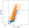 |
Fig. 1. Colour-magnitude diagram (CMD) of the RSGs in the LMC using 2MASS photometric data. The dashed lines define the photometric RSG limits from Yang et al. (2021), modified by increasing the slope of the right diagonal line. The orange points show the sources we kept in our final sample. |
We removed foreground sources using the LMC membership criteria from Jiménez-Arranz et al. (2023), in which they present a kinematic analysis using Gaia DR3 data, with a probability PLMC > 0.26. Six of our sources did not exist in the probability catalogue of Jiménez-Arranz et al. (2023). We checked whether the proper motions and parallax of the targets followed the distribution of probable members and removed 5 targets with PMRA > 2.6 mas yr−1. Figure 2 shows the distribution of proper motions and parallax, and the vertical dotted line shows the mentioned limit in PMRA. We also kept 13 targets without Gaia DR3 data (since it is uncertain whether they are foreground). We required that all sources have photometry in at least one band at λ > 8 μm to properly model the infrared excess of the dust. The majority of our sources have at least two observations in that range. For those that had only one, we required that they have photometry from Spitzer [8.0] or W3. Figure 3 shows the spatial distribution of the final and clean sample of 2219 RSG candidates, including the dust-enshrouded RSG WOH G64 (Levesque et al. 2009), which was explicitly added, as it did not exist in our source catalogues.
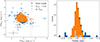 |
Fig. 2. Proper motions in Dec and RA (left) and distribution of parallaxes (right). The blue points show the initial RSG sample, and the orange points show the LMC members after applying the probability criteria from Jiménez-Arranz et al. (2023) with PLMC > 0.26. The grey points indicate sources without a probability measurement from Jiménez-Arranz et al. (2023). Sources located right of the dotted vertical line were considered to be foreground. |
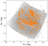 |
Fig. 3. Spatial distribution of the final RSG sample in the LMC (orange points). The background targets (grey) are the complete sample of all sources from Yang et al. (2021). |
We corrected for foreground Galactic extinction using the extinction law and values from Wang & Chen (2019) with RV = 3.1 and E(B − V) = 0.08 mag for the LMC (Massey et al. 2007). For the OGLE I band, we used the individually determined extinction values provided by the OGLE-III shallow survey for each target (Ulaczyk et al. 2012). We calculated the luminosity of each RSG by integrating the observed spectral energy distribution (SED), L = 4πd2∫Fλdλ, with a distance to the LMC d = 49.59 ± 0.63 kpc (Pietrzyński et al. 2019). We used the trapezium method to integrate the SED. Even though the observational data did not cover the whole spectrum, the SED beyond 24 μm does not significantly contribute to the total flux. Additionally, we computed the luminosity by integrating the whole SED of the best-fit model (described in the following section). The results agreed well (≲1% difference, reaching up to around 2% for the most luminous sources). Combination of the photometric and distance errors resulted in an error in luminosity below 2%. Figure 4 shows the luminosity distribution. We should note that the tip of the red giant branch (TRGB) defines the lower limit in Ks mag (Yang et al. 2021), which results in low-luminosity sources. The least luminous RSG in our sample, confirmed by spectroscopy (González-Fernández et al. 2015), has log(L/L⊙) ≃ 4. We used this additional cut in our study of RSG mass-loss rates to avoid contamination by lower-mass stars, such as red helium-burning stars.
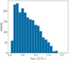 |
Fig. 4. Luminosity distribution of the RSG candidate sample. |
We calculated the effective temperatures, Teff in K, using the empirical relation for RSGs in the LMC from Britavskiy et al. (2019),
 (1)
(1)
with the observed J − Ks colour corrected for a total extinction of E(B − V) = 0.13 mag (internal and foreground; Massey et al. 2007), with an additional assumed circumstellar extinction of AV = 0.1 mag. Sources with low optical depth (τV < 0.1) have a corresponding CSM AV ≃ 0.01 mag (e.g. Kochanek et al. 2012); in more extreme cases, AV ≃ 1 mag. We checked the effect of these two values on Teff, and the difference was ≤3%. Equation (1) is valid for 0.8 < (J − Ks)0 < 1.4 mag; therefore, we did not calculate temperatures for sources with redder colours. In our sample, 118 sources had bluer colours (0.7 < (J − Ks)0 ≤ 0.8 mag), only 12 of which had log(L/L⊙) > 4. We therefore did not exclude them as they do not affect our results.
3. Dust shell models
3.1. Model parameters
We used the 1D radiative transfer code DUSTY (V4)1 from Ivezic & Elitzur (1997) to model the SEDs of our sources. DUSTY solves the radiative transfer equations for a central source inside a dust shell of certain optical depth, τV at λ = 0.55 μm in our case. We assumed a spherically symmetric dust shell extending to 104 times the inner radius, Rin. This value is commonly adopted so that the dust density is low enough at the outer limit so that it does not affect the spectrum.
3.1.1. Density distribution
We assumed steady-state winds with a constant terminal outflow velocity, v∞, and a density distribution of the dust shell falling off as ρ ∝ r−2. Outflow wind speeds of RSGs are estimated to be ∼20 − 30 km s−1 based on maser emission measurements (Richards et al. 1998; van Loon et al. 2001; Marshall et al. 2004). According to radiatively driven wind theory, the terminal outflow velocity scales with luminosity as v∞ ∝ L1/4 (van Loon 2000). We assumed 30 km s−1 for the most luminous RSG of our sample and rescaled accordingly for the wind speeds of the rest of the RSGs, v∞ = 30 (L/Lmax)1/4. For the LMC, Goldman et al. (2017) also derived a scaling relation between wind speed and luminosity by measuring the wind speeds from maser emission and found v∞ = 0.118 L0.4. However, this relation yields low values, v∞ ≲ 10 km s−1 for stars with L < 105 L⊙. In addition, Beasor & Smith (2022) suggested that some of the stars studied by Goldman et al. (2017) are luminous AGB stars and not RSGs. We chose to use the scaling by van Loon (2000), even though the dust-driven wind theory may not explain the mechanism in RSGs, since the empirical correlation of v∞ with L by Goldman et al. (2017) needs improvement. Considering the linear relation of the mass-loss rate with the outflow velocity, this assumption does not affect our results significantly. We also note that Goldman et al. (2017) provided a metallicity dependence on their mentioned relation, which Wang et al. (2021) then applied the low-metallicity LMC relation to their high-metallicity sample in M31 and M33.
Then, we calculated the mass-loss rate as (Beasor & Davies 2016)
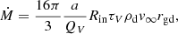 (2)
(2)
where a/QV is the ratio of the dust grain radius over the extinction efficiency at the V band, ρd is the bulk density, Rin is the inner shell radius, and rgd is the gas-to-dust ratio. We note that DUSTY has Rin as an output for a given luminosity of 104 L⊙, and the inner radius is scaled as Rin ∝ L1/2 (see DUSTY manual Sect. 4.12); thus, we rescaled each best-fit model radius as ![Mathematical equation: $ R_{\mathrm{in}} = R_{\mathrm{in}}^{\mathrm{DUSTY}} [{L}/(10^4\,L_\odot)]^{1/2} $](/articles/aa/full_html/2024/06/aa49383-24/aa49383-24-eq3.gif) . We used an average value for the gas-to-dust ratio of the LMC,
. We used an average value for the gas-to-dust ratio of the LMC,  (Clark et al. 2023).
We also opted for the numerical solution for radiatively driven winds (RDW) to test our results and compared it with the steady-state wind assumption. The full dynamics calculations can be found in Ivezic & Elitzur (1995), Elitzur & Ivezić (2001) and references therein. The analytic approximation is shown below for reference,
![Mathematical equation: $$ \begin{aligned} \eta ({ y}) \propto \frac{1}{{ y}^2}\left[\frac{{ y}}{{ y}-1+\left(v_1/v_{\rm e}\right)^2}\right]^{1/2}, \end{aligned} $$](/articles/aa/full_html/2024/06/aa49383-24/aa49383-24-eq5.gif) (3)
(3)
where η is the dimensionless density profile normalised according to ∫ηdy = 1, y ≡ r/Rin with Rin the inner shell radius, and v1 and ve the initial and final expansion velocities, respectively. The mass-loss rate for RDW is given as an output from DUSTY for L = 104 L⊙, rgd = 200 and ρd = 3 g cm−3, demanding a rescaling according to the dust-driven wind relation by van Loon (2000),
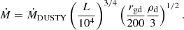 (4)
(4)
We should note that McDonald et al. (2011) have an error in their Ṁ relation (Eq. (1) in their paper): They divide the dust-to-gas ratio ψ by 200 instead of 1/200. This erroneous equation was also applied by Yang et al. (2023), with an index of −1/2 instead of 1/2 for the gas-to-dust ratio. Application of the correct relation would yield higher mass-loss rates by a factor of 5 or 0.7 dex in logarithmic space in the Yang et al. (2023) result.
3.1.2. Dust composition
The dust grain composition affects the interaction of radiation with the dust shell and is observed in the output SED. Observations of RSGs indicate O-rich silicate features at roughly 10 μm and 18 μm, as shown in previous works (e.g. van Loon et al. 2005; Groenewegen et al. 2009; Verhoelst et al. 2009; Sargent et al. 2011; Beasor & Davies 2016; Goldman et al. 2017). We opted for the astronomical silicate of Draine & Lee (1984) with a dust bulk density of ρd = 3.3 g cm−3.
3.1.3. Grain size distribution
We used the modified Mathis-Rumpl-Nordsieck (MRN) distribution n(a)∝a−q for amin ≤ a ≤ amax (Mathis et al. 1977). Observations of VY CMa, a dust-enshrouded RSG, yielded an average grain radius of 0.5 μm (Scicluna et al. 2015), while other studies showed that grain sizes are in the range of 0.1 − 1 μm (Smith et al. 2001; Groenewegen et al. 2009; Haubois et al. 2019). Thus, we opted for amin = 0.1 μm, amax = 1 μm and q = 3, even though the grain size in the range of [0.1, 0.5] does not significantly affect the mass-loss rate (Beasor & Davies 2016).
A broader MRN distribution with a grain size in the range 0.01 − 1 μm and q = 3.5 has been applied for different populations of RSGs by Verhoelst et al. (2009), Liu et al. (2017), Wang et al. (2021). Moreover, Ohnaka et al. (2008) determined grain sizes in that range from their best-fit model of WOH G64. This profile has an average grain size of approximately 0.02 − 0.03 μm, which affects the extinction efficiency, QV (see Fig. 4 in Wang et al. 2021). Since it is difficult to infer a grain size from photometric data, we used this broader range of the modified MRN distribution to compare with our main assumption and to examine its effect on the mass-loss rate.
3.1.4. Stellar atmosphere models, Teff
We used the MARCS model atmospheres (Gustafsson et al. 2008) as input SEDs for the central source. We chose typical RSG parameters: a stellar mass of 15 M⊙, a surface gravity log g = 0, interpolated models with metallicity [Z]= − 0.38, consistent with the metallicity of RSGs in the LMC, [Z]= − 0.37 ± 0.14 (Davies et al. 2015), and effective temperatures, Teff, in the range of [3300, 4500] with a step of 100 K. We interpolated the models between 4000 and 4500 K to create models with a step of 100 K, which are not available by default. We chose the commonly adopted value for RSGs of log g = 0, although it can be as low as approximately −0.5 (e.g. Davies et al. 2015). However, this affects the peak of the SED due to line blanketing, shifting it to appear slightly cooler for higher log g, and it is degenerate with the effective temperature. Since we could not constrain both parameters, we chose to fix the value for log g. This can affect the derived Teff from DUSTY, but we used Eq. (1) to calculate the Teff of our sources. A varied Teff in DUSTY leaves the mass-loss rate almost unaffected (Beasor & Davies 2016). We then resampled the MARCS model surface fluxes by decreasing the resolution, and we matched them with the custom DUSTY wavelength grid. Since MARCS models extend up to 20 μm, we extrapolated longer wavelength ranges using a blackbody.
3.1.5. Inner dust shell temperature Tin and optical depth τV
We set the dust temperature at the inner radius of the dust shell, Tin, in the range of [400, 1200] with a step of 100 K. We also set the sublimation temperature to 1200 K, which is considered to be an approximation for silicate dust (Gail et al. 1984, 2020; Gail & Sedlmayr 1999).
The optical depth, τV, was varied using 30 logarithmic steps in the range of [0.001, 0.1], 70 steps in the range of [0.1, 1], and 99 in [1, 10].
In total, we created 23 049 models in which we varied the mentioned parameters to optimise the data fitting.
3.2. Spectral energy distribution fitting
First, we created synthetic fluxes by convolving the model spectrum with the filter profiles of each observational instrument3. We then calculated the minimum modified χ2,  , as defined below (Yang et al. 2023),
![Mathematical equation: $$ \begin{aligned} \chi ^2_{\rm mod}=\frac{1}{N-p-1} \sum {\frac{[1-F(\mathrm{Model}, \lambda )/F(\mathrm{Obs}, \lambda )]^2}{F(\mathrm{Model}, \lambda )/F(\mathrm{Obs}, \lambda )}}, \end{aligned} $$](/articles/aa/full_html/2024/06/aa49383-24/aa49383-24-eq8.gif) (5)
(5)
where F(λ) is the flux at a specific wavelength, N is the number of photometric data of each source, and p is the free parameters. The output flux of DUSTY is given at the outer dust shell radius, Rout = 104 Rin, so to compare with the observed flux on Earth,
 (6)
(6)
where d is the distance to the source-galaxy (d = dLMC).
We used this definition of minimum χ2 to balance the contribution of fluxes from both the optical and the infrared. A regular χ2 would barely account for the infrared flux, which is crucial for determining the dust properties, and it would weight the optical photometry much more. The modified χ2 treats all wavelengths equally since it depends on the ratio of the model over the observation instead of the difference (see Sect. 3.2 in Yang et al. 2023, for a more detailed explanation).
We determined the errors on the best-fit parameters as in Beasor & Davies (2016), but since we have a different definition of the minimum χ2, we defined them by the models within the minimum  . This is a crude estimation of the errors and does not account for all the uncertainties that lie in every assumption that is made.
Figure 5 shows six example SEDs. In the top row, we included two optically thin RSGs without IR excess, demonstrating the absence of a dust shell. In the middle row, the mid-IR excess shows the presence of a dust shell emitting in this wavelength range, and the bump at around 10 μm reveals the presence of silicate dust. In the bottom row, we present some peculiar examples that could not be properly fit by a model with a significant IR excess or a UV excess, indicating a binary candidate. The bottom left source is a supergiant B[e] star (ID 225) that passed the photometric criteria along with two more stars (IDs 192, 706), found in the catalogue of Kraus (2019). However, these stars are not included in our analysis of mass-loss rates because their model fits are poor, as we explain in the following section. We also found 57 matches of our sample with the Spitzer InfraRed Spectrograph (IRS) Enhanced Products (Houck et al. 2004), using a 1″ radius, to visually validate our SED fits; 3 of these matches are shown in Fig. 5.
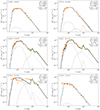 |
Fig. 5. Examples of SED fits of two optically thin (top row), two dusty (middle), and two peculiar (bottom row) RSGs. The orange diamonds show the observations, and the black line is the best-fit model consisting of the attenuated flux (dashed light blue), the scattered flux (dot-dashed grey) and dust emission (dotted brown). The green curve represents the Spitzer IRS spectrum. The coordinates of each source are shown in the top left corner. |
4. Results
Fitting the observed SEDs with the DUSTY models, we obtained the dust shell parameters and mass-loss rates for each RSG. Figure 6 shows the histograms of the minimum  and the best-fit τV. We consider models with
  as a good fit, where the standard deviation is σχ2 = 0.41. Moreover, we do not present the parameters of 36 RSG candidates, as their SED could not be fit by any model of the grid. The average optical depth is τV = 0.09. Figure 7 shows a histogram of the best-fit model effective temperatures on the left along with two colour-temperature, Teff(J − Ks), LMC empirical prescriptions (Neugent et al. 2012; Britavskiy et al. 2019) applied to our sample. In this study, we proceed with the relation from Britavskiy et al. (2019) because it was calibrated on temperature measurements from i-band spectra, which are more reliable than TiO-band spectra (for a discussion see Davies et al. 2013; de Wit et al. 2024). The DUSTYTeff reveals a discrepancy with those resulting from Eq. (1). One reason is that we used the modified χ2, which enhances the weight in the mid-IR part of the SED, and it looses some weight in the optical to the near-infrared, where the effective temperature affects the SED more strongly. This suggests that our derived Teff from DUSTY are less reliable. Table 2 includes our final catalogue of RSG candidates in the LMC with their coordinates, photometry, Gaia astrometry, spectral classifications from the literature, and the parameters derived from this work.
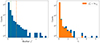 |
Fig. 6. Distributions of SED fitting parameters. Left: distribution of the minimum |


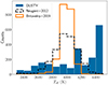 |
Fig. 7. Distribution of the best-fit effective temperatures from DUSTY. The lines show the applied J − Ks empirical prescriptions from Neugent et al. (2012) (orange) and Britavskiy et al. (2019) (dashed black) to our sample. |
Properties and derived parameters of RSG candidates in the LMC.
4.1. Mass-loss rates
We present the derived mass-loss rates versus the luminosities in Fig. 8. We exclude 94 sources with best-fit models of  , which suggests that their derived Ṁ may not be reliable. The colour bar shows the best-fit optical depth, τV, of each source. The uncertainties are propagated from the error models defined in the previous section and the error on the gas-to-dust ratio. We note that the relative error becomes higher at log(L/L⊙) < 4.5. The grey triangles show the upper limits for sources with τV ≤ 0.002. In this regime, the different model SEDs are indistinguishable and do not show any significant indications of dust in the CSM. We also mark the RSGs confirmed by spectral classification from the catalogues of Yang et al. (2021) and González-Fernández et al. (2015). The red star indicates WOH G64, a dust-enshrouded RSG. However, the grain size for this RSG should be lower than the range we considered in Sect. 3, resulting in a higher Ṁ, as we discuss in Appendix A.
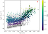 |
Fig. 8. Derived mass-loss rate as a function of the luminosity of each RSG candidate in the LMC. The colour bar shows the best-fit τV. The grey triangles represent the upper limits of targets fitted with the lowest values of the optical depth grid, and the open circles indicate the RSGs with spectral classifications. The dust-enshrouded RSG, WOH G64, is labelled with a red star. The position of the kink is shown with a dashed vertical line at log(L/L⊙) = 4.42. |
The average mass-loss rate is Ṁ ≃ 6.4 × 10⁻⁷ M⊙ yr−1, while for log(L/L⊙) > 4, it is Ṁ ≃ 9.3 × 10⁻⁷ M⊙ yr−1. The latter corresponds to a mass of ∼0.1 − 1 M⊙ that is lost throughout the lifetime of an RSG, which is presumed to be 105 − 106 yr, and an average dust-production rate of ∼3.6 × 10⁻⁹ M⊙ yr−1. There is a noteworthy dispersion at log(L/L⊙) ≲ 4.1, but these sources may not be RSGs, as previously mentioned. More significantly, we observe an enhancement of mass loss at log(L/L⊙) ≃ 4.4 that appears as an increase in the slope of the Ṁ(L) relation or a kink, similar to recent findings in the SMC (Yang et al. 2023). Finally, the mass loss additionally correlates with the effective temperature, the dust temperature, and variability among other properties of the RSG and CSM, which we further discuss in the following subsections.
4.2. Variability
We used the epoch photometry from NEOWISE to calculate the median absolute deviation (MAD) of W1 [3.4] band and examined the correlation with luminosity, as was done by Yang et al. (2023). We show this correlation in Fig. 9. The MAD value for W1 [3.4] typically indicates the intrinsic variability of an RSG (Yang et al. 2018). We observe that the trend of MAD with L is nearly identical to the trend of the Ṁ(L). Thus, the variability appears to correlate with the enhancement of mass loss observed at the turning point around log(L/L⊙) = 4.4. There is also high variability for some sources at lower luminosity than the turning point, which we discuss further in Sect. 5.1. Finally, for the extreme assumption that RSGs could vary bolometrically up to 1 mag, it would induce a variation in the luminosity of up to 0.2 dex (Beasor et al. 2021).
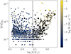 |
Fig. 9. MAD of W1 band vs. luminosity diagram. The colour bar shows the corresponding mass-loss rate of each source. The open circles indicate the RSGs with spectral classifications, and the dashed line represents the position of the kink, as in Fig. 8. |
4.3. Binarity
Red supergiants can be part of a binary system with an OB companion (e.g. Neugent et al. 2019). Binary RSGs consist of around 20% of the total RSG population (Neugent et al. 2020; Patrick et al. 2022). We further investigated this fraction in our sample following the B − V versus U − B colour diagram from Neugent et al. (2020), which distinguishes the binary population. We considered sources with U − B < 0.7 mag as binary candidates. This resulted in a fraction of 21% binary candidates in our complete sample of sources with UBV photometry, and it strongly agrees with Neugent et al. (2020). Figure 10 shows the B − V versus U − B colour diagram of these sources, indicating those existing in the Neugent et al. (2020) catalogue with a binary probability Pbin > 0.6. We demonstrate the Ṁ−L result, and we indicate the binary candidates with orange circles in Fig. 11.
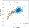 |
Fig. 10. Colour-colour diagram of U − B and B − V. The blue points show all sources with UBV photometry. The orange circles indicate RSGs from Neugent et al. (2020) with a probability of an OB companion Pbin > 0.6. The vertical dotted line corresponds to the limit applied to separate probable binary from single RSG. |
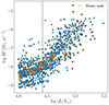 |
Fig. 11. Same as Fig. 8, but for log(L/L⊙) > 4, indicating the binary candidates (U − B < 0.7 mag) with orange circles. |
4.4. Ṁ(L,Teff)
In addition to the luminosity, we examined the dependence of the mass-loss rate on the effective temperature calculated using Eq. (1) with an equal uncertainty of 140 K for each source (Britavskiy et al. 2019). The right panel of Fig. 12 shows that these two properties are anti-correlated, which agrees with the findings of de Jager et al. (1988) and van Loon et al. (2005). The Teff(J − Ks) relation from Neugent et al. (2012) based on synthetic models yields a similar correlation with Ṁ, which is less steep since it predicts a broader range of Teff. However, we proceeded with the relation from Britavskiy et al. (2019) because it is empirically derived rather than from synthetic models (for a comparison between different Teff prescriptions see de Wit et al. 2024). We fitted a broken relation dependent on both luminosity and effective temperature,
 (7)
(7)
 |
Fig. 12. Mass-loss rates vs. luminosity (left) and effective temperature (right) calculated from Eq. (1). The magenta points correspond to the prediction of the derived Ṁ(L,Teff) relation, Eq. (7), showing the correlation of the mass-loss rate as a function of the luminosity and effective temperature. |
with Ṁ the mass-loss rate in M⊙ yr−1, L the luminosity in L⊙, and Teff the effective temperature in K. We present the best-fit parameters in Table 3. We derived the relation at log L/L⊙ > 4, roughly above the luminosity limit for RSGs in the LMC. The limit could be slightly higher, but regardless, the slope does not change up to the position of the kink. The left panel of Fig. 12 shows the relation we applied to our sources compared with the derived Ṁ.
4.5. Steady-state versus radiatively driven winds
Previous studies have shown a large discrepancy in their obtained Ṁ (cf. van Loon et al. 2005; Goldman et al. 2017; Beasor et al. 2020; Yang et al. 2023). In Fig. 13, we compare the resulting Ṁ of steady-state winds versus RDW as a function of L. The steady-state wind case has a slightly steeper slope than the RDW, mainly due to the different assumptions about the dependence of the outflow velocity on the luminosity. We corrected the Ṁ(L) relation from Yang et al. (2023) by adding 0.7 dex to their log Ṁ, and we present it in the same figure with the black line. Their result of the SMC matches ours in the LMC, indicating that RSG winds are metallicity independent, apart from the luminosity limit of the kink (see Sect. 5.3). The bottom panel demonstrates the Ṁ ratio of the two modes. There is a significant difference in the results of the two assumptions by two to three orders of magnitude. The result from RDW would strip off most of the luminous RSGs and shift them to higher Teff in the HR diagram, which is not confirmed by observations (Zapartas et al., in prep.).
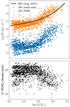 |
Fig. 13. Comparison between the resulting mass-loss rates of steady-state winds and RDW. Top: mass-loss rate vs. luminosity. The results from steady-state winds and RDW are indicated with blue and orange, respectively. The solid line shows the relation by Yang et al. (2023) in the SMC corrected by adding 0.7 dex. Bottom: the ratio of the results of the two modes. |
4.6. Grain size MRN [0.01, 1] versus [0.1, 1]
We used the modified MRN grain size distribution in the range of [0.01, 1] μm to compare with our assumption of [0.1, 1] μm. The lower size distribution has an average grain size of around 0.02 μm, and the average ratio a/QV becomes higher by a factor of ∼20 (see Fig. 4 in Wang et al. 2021), which linearly affects the Ṁ. The top panel of Fig. 14 shows the Ṁ ratio assuming a grain size in the range of [0.01, 1] over the range of [0.1, 1] μm. This assumption results in a higher Ṁ by a factor of around 25−30. The bottom panel of Fig. 14 shows that the larger grain size appears to have slightly better-fit models for the highest luminosity sources. Despite this, the effect of grain sizes on the SED is indistinguishable and can therefore not be obtained with precision. We performed the same comparison using the RDW mode in DUSTY. We found an opposite correlation in this case; the smaller grain size yields an Ṁ lower by a factor of ∼0.8. This may have to do with the different dependence of the Ṁ from RDW on the extinction efficiency Q (see Elitzur & Ivezić 2001). We present the derived Ṁ(L,Teff) relation for the mentioned assumptions in Appendix B.
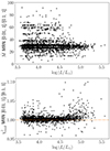 |
Fig. 14. Effect of the grain size distribution on the mass-loss rate for a range of luminosities. Top: ratio of the mass-loss rates assuming an MRN grain size distribution in the range [0.01, 1] μm over the distribution in the range [0.1, 1] μm. Bottom: ratio of the minimum |

5. Discussion
The most commonly used RSG Ṁ prescription is from de Jager et al. (1988). Despite their limited sample size of 15 stars, it provides satisfactory results at solar metallicity (Mauron & Josselin 2011). We derived an Ṁ(L,Teff) relation with a similar correlation with luminosity and effective temperature as de Jager et al. (1988). The anti-correlation with Teff is expected because the RSGs expand their envelope as they evolve up the Hayashi track, where they steeply increase in luminosity and slightly drop in Teff.
It is noteworthy that we found a knee-like shape or kink of the mass-loss rate as a function of the luminosity, as presented in the previous section. Modelling an equally large, unbiased sample, Yang et al. (2023) demonstrated that a similar turning point is correlated with the variability. Studying a sample of 42 RSGs, Humphreys et al. (2020) found a transition in the Ṁ(L) relation at approximately log(L/L⊙) = 5 and attributed it to instabilities in the atmosphere of evolved RSGs. Thus, the kink may indicate a change in the physical mechanism. Figure 9 shows that the kink strongly correlates with the intrinsic photometric variability of the RSG. We could hypothesise that the variability is due to pulsations of the RSG in the stellar atmosphere, expelling gas to altitudes at which molecules can condense and form dust. In addition to this, increased radiation pressure on the dust shell could arise at a specific luminosity limit (Vink & Sabhahit 2023). If turbulence is the dominant mass-loss mechanism (Kee et al. 2021), measurements of the turbulent velocity versus the luminosity could provide better insight into the instabilities of the stellar atmosphere. It might be argued that sources with lower L than the position of the kink are not RSGs and that these stars may be bound to a different physical driving mechanism. However, Fig. 8 demonstrates that there are spectroscopically confirmed RSGs below that point.
We observe a high dispersion in the mass-loss rates (see Fig. 8), which could be due to variability, or it could arise from different stellar parameters that affect the Ṁ, such as different Teff. We showed in Fig. 12 that Teff partially compensates for the dispersion. In addition, different inner dust shell temperatures, which define the distance of the dust shell from the star, could contribute to it. A lower dust temperature corresponds to higher Rin resulting in higher Ṁ (see Eq. (2)). Moreover, Beasor et al. (2020) found a correlation with the initial mass, as they targeted coeval RSGs in clusters. Different turbulent or outflow speeds could also affect this dispersion (e.g. Kee et al. 2021). Finally, the grain size and gas-to-dust ratio, which we have assumed to be uniform for our whole sample, can vary between RSGs, which might affect the Ṁ spread.
5.1. Red helium-burning stars
At log(L/L⊙) < 4.2, we find enhanced variability for a fraction of sources (∼6%), mainly towards the lower luminosities of the sample. These sources are likely red helium-burning (RHeB) stars with masses < 8 M⊙. These stars are at the evolutionary point after the red giant phase and before becoming AGB stars when they perform a loop in the HR diagram on the horizontal branch. They undergo pulsations (Kippenhahn et al. 2013), which could contribute to the observed variability. Although not certain, the wind mechanism could follow the RDW theory, similarly to the AGB phase. This potentially explains why our steady-wind assumption creates a high dispersion in the Ṁ results, in contrast to the RDW case, where they are more uniform (see Fig. 13). Finally, as mentioned previously, there may still be AGB star contamination despite the constraints applied to the initial sample.
5.2. Luminous outliers in the Ṁ(L) relation
We searched the literature for the sources that appear as outliers in Fig. 8: (i) 5 sources with τV > 2 and log(L/L⊙) > 4.4, and (ii) 11 sources with log(L/L⊙) > 5.2. (i) ID 807 and ID 1348 are classified by photometry as long-period variables (LPVs) and O-rich AGB stars (Soszyński et al. 2009), and ID 1139 is an M-type giant by spectroscopy (de Wit et al. 2023). The other 2 sources are M-type supergiants (Wood et al. 1983; González-Fernández et al. 2015). More specifically, we found that ID 2107, W61 7-8, with spectral type M3.5Ia (González-Fernández et al. 2015), is a dust-enshrouded RSG according to criteria from Beasor & Smith (2022) with Ks − W3 = 3.68 mag. We did not have more RSGs with Ks − W3 > 3.4 mag, mainly because the CMD selection criteria from Neugent et al. (2012) and Ren et al. (2021) remove sources with high J − Ks values, which rejected dust-enshrouded RSGs. (ii) Three of them (IDs 408, 1829, and 1866) do not have any classification, 2 are classified as M-type supergiants by photometry (Westerlund et al. 1981), and the rest are classified as M-type supergiants by spectroscopy (Wood et al. 1983; Reid & Mould 1985; van Loon et al. 2005; González-Fernández et al. 2015; de Wit et al. 2023). Five of these are binary candidates, as we indicate in Fig. 11. Finally, ID 1786, [W60] B90, is an extreme RSG, with evidence of a bow shock, undergoing episodic mass loss (Munoz-Sanchez, in prep.).
5.3. Comparison with other works: Zoo of mass-loss rate prescriptions
There is a plethora of Ṁ prescriptions for RSGs with different assumptions and results. Our sample of RSGs with derived Ṁ is one of the largest, among others (Wang et al. 2021; Yang et al. 2023; Wen et al. 2024). In Table 4, we present the prescriptions from the literature to which we compared our work. In addition to luminosity, some relations depend on the effective temperature, the stellar radius, the initial or current mass, the pulsation period P, or the gas-to-dust ratio. All are empirical relations, except for the analytic solution by Kee et al. (2021), who assumed that atmospheric turbulence is the dominant driving mechanism for mass loss and that it strongly depends on the turbulent speed, vturb. The luminosity L and the mass M are in solar units, and the temperature Teff is in K. To compare them properly, we applied the average Teff of our sample to all prescriptions and their suggested optimal parameters for the rest.
Mass-loss rate prescriptions from different works.
In Fig. 15 we compare the different relations with our results. Many uncertainties arise between different studies, for instance different samples, photometric bands used, metallicity, radiative-transport models, assumptions on the mass-loss mechanism, grain size, and gas-to-dust ratio. Our results agree better with Beasor et al. (2023), who used similar assumptions, although they had a smaller sample and luminosity range. The differences with Beasor et al. (2023) lie within the errors and slight variations of the assumptions, such as the gas-to-dust ratio, the grain size and the outflow speed. The de Jager et al. (1988) relation overestimates the Ṁ at lower luminosities and is closer to ours at log(L/L⊙) > 4.8, but less steep. Humphreys et al. (2020) found slightly lower Ṁ than de Jager et al. (1988) at 4 < log(L/L⊙) < 5, with an enhancement in the mass loss at log(L/L⊙) > 5. Yang et al. (2023), van Loon et al. (2005), and especially Goldman et al. (2017) found much higher Ṁ due to the RDW assumption in DUSTY, which results in two to three orders of magnitude higher Ṁ (see Fig. 13). More specifically, van Loon et al. (2005) used the RDW analytic mode on DUSTY, which results in lower values than the fully numerical solution of RDW, as we verified. However, the analytic approximation is only applicable in the case of negligible drift (Elitzur & Ivezić 2001). Goldman et al. (2017) and van Loon et al. (2005) studied dust-enshrouded RSGs, and Goldman et al. (2017) included AGB stars, which are expected to have high Ṁ. Almost none of these studies found a kink in their results, mainly because their samples were small and biased towards high luminosities.
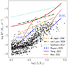 |
Fig. 15. Comparison of our Ṁ(L) result (open circles) with prescriptions from previous works presented in Table 4. The two lines from Beasor et al. (2020) correspond to an initial mass of 10 M⊙ and 20 M⊙, and the same holds for Kee et al. (2021), but represents the current mass. |
We found that the kink is located at log(L/L⊙)≃4.4, whereas in the SMC, it was found at log(L/L⊙) = 4.6 (Yang et al. 2023). We speculate that this luminosity shift is related to metallicity since the SMC is a lower-metallicity environment with [Z]SMC = −0.53 (Davies et al. 2015). Metallicity could affect this physical procedure if the enhanced mass loss were due to instabilities in the atmosphere of RSGs. A lower Z results in more compact stars during the main sequence, meaning a more massive core for the same initial mass and a higher L for RSGs. This shifts the luminosity limit for RSGs and could explain the shift of the kink. In addition, lower Z stars have weaker radiatively driven winds during the main sequence (Vink et al. 2001), slowing down their rotation at a slower rate. The higher rotation results in enhanced mixing and a larger core (Meynet et al. 2006), which again produces a more luminous RSG for the same initial mass.
Finally, our result agrees with the determined mass-loss rates of four RSGs from the observations of CO rotational line emission (Decin et al. 2024), which provides confidence in our assumptions. The theoretical relation by Kee et al. (2021) predicts higher Ṁ for low masses and has a similar slope as ours at high L (see Fig. 15). A further investigation of the Ṁ with observational and theoretical methods and robust samples could provide more solid support for the existing empirical relations.
Wen et al. (2024) recently published a similar study of RSGs in the LMC. They used two-dimensional models from 2-DUST (Ueta & Meixner 2003) and steady-state winds, finding similar mass-loss rates. They also indicated the same position of the kink in the Ṁ−L relation. It is reassuring that two independent methods provide similar results. However, there are a few notable differences. Firstly, they only used the RSG catalogue from Ren et al. (2021) and did not remove foreground sources existing in that catalogue. Secondly, they fit sources without photometry at λ > 8 μm with low optical depth models, whereas we rejected them. Their empirical relation is therefore based on some erroneous mass-loss rate measurements. Thirdly, a significant difference is that we provide an Ṁ prescription dependent on both L and Teff, explaining a large part of the dispersion in the results. Some other minor differences are that they used rgd = 500 from Riebel et al. (2012), who used this abstract value without deriving it, but it is within our estimated errors, and v∞ = 10 km s−1, which could be low for some extreme RSGs with v∞ = 20 − 30 km s−1, as we discussed. Finally, they considered that sources with log(L/L⊙) < 4.5 and high Ṁ are pseudo sources or are affected by nearby sources. This may be valid for some cases, but we showed that some of these have increased variability, indicating another type of star (e.g. RHeB giant). In summary, we provide a better-established Ṁ(L,Teff) relation based on a cleaner RSG catalogue and an explanation for the scatter at both low L and high L sources.
5.4. Caveats
Several caveats arise from DUSTY and the assumptions we made in our RSG sample. Deriving the mass loss from the circumstellar dust of RSGs, appearing in their SED as excess at λ > 3.6 μm, constitutes a snapshot and has uncertainties. It neglects that RSGs can undergo episodic mass loss, forming a thick shell. However, these are rare events that occur in the late stages of RSGs. Furthermore, the gas-to-dust ratio is not uniform in every region of a galaxy. More luminous RSGs may have higher rgd (Goldman et al. 2017). However, it varies by less than an order of magnitude in the LMC, which would not affect the estimated Ṁ significantly, in contrast to the case of the SMC, in which the gas-to-dust ratio varies by a factor of ∼20 (Clark et al. 2023).
The assumption of a spherically symmetric dust shell is not realistic. Dust around RSGs is clumped and asymmetric (Smith et al. 2001; Scicluna et al. 2015). However, clumping has a minor effect on the Ṁ (Beasor & Davies 2016). Luminosity measurements could be affected in the case of dense shells, resulting in higher or lower L, depending on the orientation of the clumps. This occurred in WOH G64, the luminosity of which is higher when integrating the SED than what Ohnaka et al. (2008) inferred by modelling the dusty torus.
Binarity would affect the derived mass loss under the assumptions we made. The hotter OB companion could alter the shape of the dust shell or even heat and destroy part of the dust with its radiation field. We found that the impact of binaries on our derived Ṁ(L,Teff) relation was negligible. We show this in Appendix C, and we provide a more conservative Ṁ(L,Teff) relation by fitting only the probable single RSGs. We should mention that this fraction represents the current binary RSGs and does not exclude the binary history of the probable single RSGs with accretion of mass or merging (e.g. Zapartas et al. 2019). We observed that most of the high L binary candidates appear to have lower Ṁ than the probable single ones for the same L (see Fig. 11). This means that their SED exhibits a lower IR excess, which could originate from the destruction of dust by the OB companion. Finally, due to their UV excess, their derived L is slightly higher, and they appear more to the right in the Ṁ−L plot than if they were single stars.
6. Summary and conclusion
We have assembled and analysed a large, clean, and unbiased sample of 2219 RSG candidates in the LMC, 1376 of which have log(L/L⊙) > 4. We used photometry in 49 filters ranging from the UV to the mid-IR to construct SEDs, from which we measured luminosities and effective temperatures, and we derived the mass-loss rates for these sources using the radiative code DUSTY. The average mass-loss rate is 6.4 × 10⁻⁷ M⊙ yr−1, while for log(L/L⊙) > 4, it is 9.3 × 10⁻⁷ M⊙ yr−1. The latter corresponds to a mass of ∼0.1 − 1 M⊙ lost throughout the lifetime of an RSG, presumed to be 105 − 106 yr, and to an average dust-production rate of ∼3.6 × 10⁻⁹ M⊙ yr−1.
We presented an accurate Ṁ relation as a function of both L and Teff, finding it to be proportional to L and inversely proportional to the Teff. We found a turning point or kink in the Ṁ−L relation similar to the one in the SMC (Yang et al. 2023), but at lower luminosity, log(L/L⊙)≃4.4, as in Wen et al. (2024). The kink indicates an enhancement of mass loss beyond this luminosity limit, and we showed that this tightly correlates with variability. This indicates a physical mechanism that starts to dominate the RSG wind beyond this limit. Furthermore, the varying location of the kink between the SMC and LMC suggests that this enhancement depends on the metallicity.
We investigated the effect of the assumptions made in DUSTY on the resulting mass-loss rates. We found that the density distribution of the wind profile affects the RSG mass-loss rates most and that the RDW assumption causes the discrepancy of two to three orders of magnitude in the RSG mass-loss rate measurements in the literature. The RDW assumption produces unrealistically high values for quiescent mass loss in RSGs, whereas the assumption of a steady-state wind yields results that are confirmed by independent methods (e.g. measurement of gas), which have been measured for a small number of RSGs. We derived mass-loss rates for our sample using RDW that closely match the SMC rates measured by Yang et al. (2023) under this assumption. This indicates that apart from the position of the kink, RSG mass-loss rates can be independent of metallicity. Additionally, we tested the effect of the grain size in the case of a steady-state wind and found that a grain size of a < 0.1 μm increases Ṁ up to a factor of 25−30. We found a binarity fraction of 21% based on UV excess and showed that when these binary RSG are included, the derived Ṁ relation is not significantly affected.
The current investigation provided an improved method and a well-established Ṁ(L,Teff) relation compared to previous works. Repeating this exercise for the SMC, M31 and M33 following the same method and assumptions will confirm whether mass loss in RSGs depends on the metallicity. Further research on the theoretical derivation of the Ṁ−L relation, as in Kee et al. (2021), and future measurements of gas emission lines (e.g. CO; Decin et al. 2024) provide independent ways of confirming the estimated mass-loss rates.
DUSTY manual V4, https://github.com/ivezic/dusty/blob/master/release/dusty/docs/manual.pdf
The filter profiles were retrieved from http://svo2.cab.inta-csic.es/theory/fps/
Acknowledgments
K.A., A.Z.B., Sd.W., E.Z., G.M.S., and G.M. acknowledge funding support from the European Research Council (ERC) under the European Union’s Horizon 2020 research and innovation program (Grant agreement No. 772086). E.Z. also acknowledges support from the Hellenic Foundation for Research and Innovation (H.F.R.I.) under the “3rd Call for H.F.R.I. Research Projects to Support Post-Doctoral Researchers” (Project No: 7933). K.A. thanks Ming Yang for helping with the use of DUSTY and Emma Beasor for valuable discussions regarding DUSTY and the RSG wind properties. K.A. would also like to thank the participants of the VLT-FLAMES Tarantula Survey (VFTS) meeting in 2023 who provided useful questions and comments on our preliminary results.
References
- Arroyo-Torres, B., Wittkowski, M., Chiavassa, A., et al. 2015, A&A, 575, A50 [NASA ADS] [CrossRef] [EDP Sciences] [Google Scholar]
- Beasor, E. R., & Davies, B. 2016, MNRAS, 463, 1269 [NASA ADS] [CrossRef] [Google Scholar]
- Beasor, E. R., & Smith, N. 2022, ApJ, 933, 41 [NASA ADS] [CrossRef] [Google Scholar]
- Beasor, E. R., Davies, B., Smith, N., et al. 2020, MNRAS, 492, 5994 [Google Scholar]
- Beasor, E. R., Davies, B., Smith, N., Gehrz, R. D., & Figer, D. F. 2021, ApJ, 912, 16 [NASA ADS] [CrossRef] [Google Scholar]
- Beasor, E. R., Davies, B., Smith, N., et al. 2023, MNRAS, 524, 2460 [Google Scholar]
- Bianchi, L., Shiao, B., & Thilker, D. 2017, ApJS, 230, 24 [Google Scholar]
- Boyer, M. L., Srinivasan, S., van Loon, J. T., et al. 2011, AJ, 142, 103 [Google Scholar]
- Britavskiy, N., Lennon, D. J., Patrick, L. R., et al. 2019, A&A, 624, A128 [NASA ADS] [CrossRef] [EDP Sciences] [Google Scholar]
- Cioni, M. R. L., Clementini, G., Girardi, L., et al. 2011, A&A, 527, A116 [CrossRef] [EDP Sciences] [Google Scholar]
- Clark, C. J. R., Roman-Duval, J. C., Gordon, K. D., et al. 2023, ApJ, 946, 42 [NASA ADS] [CrossRef] [Google Scholar]
- Cutri, R. M., Wright, E. L., Conrow, T., et al. 2021, VizieR Online Data Catalog: II/328 [Google Scholar]
- Davies, B., & Beasor, E. R. 2020, MNRAS, 493, 468 [NASA ADS] [CrossRef] [Google Scholar]
- Davies, B., Kudritzki, R.-P., Plez, B., et al. 2013, ApJ, 767, 3 [Google Scholar]
- Davies, B., Kudritzki, R.-P., Gazak, Z., et al. 2015, ApJ, 806, 21 [NASA ADS] [CrossRef] [Google Scholar]
- Decin, L., Hony, S., de Koter, A., et al. 2006, A&A, 456, 549 [NASA ADS] [CrossRef] [EDP Sciences] [Google Scholar]
- Decin, L., Richards, A. M. S., Marchant, P., & Sana, H. 2024, A&A, 681, A17 [NASA ADS] [CrossRef] [EDP Sciences] [Google Scholar]
- de Jager, C., Nieuwenhuijzen, H., & van der Hucht, K. A. 1988, A&AS, 72, 259 [NASA ADS] [Google Scholar]
- de Wit, S., Bonanos, A. Z., Tramper, F., et al. 2023, A&A, 669, A86 [NASA ADS] [CrossRef] [EDP Sciences] [Google Scholar]
- de Wit, S., Bonanos, A. Z., Antoniadis, K., et al. 2024, A&A, in press, https://doi.org/10.1051/0004-6361/202449607 [Google Scholar]
- Draine, B. T., & Lee, H. M. 1984, ApJ, 285, 89 [NASA ADS] [CrossRef] [Google Scholar]
- Dupree, A. K., Strassmeier, K. G., Calderwood, T., et al. 2022, ApJ, 936, 18 [NASA ADS] [CrossRef] [Google Scholar]
- Eldridge, J. J., Fraser, M., Smartt, S. J., et al. 2013, MNRAS, 436, 774 [NASA ADS] [CrossRef] [Google Scholar]
- Elitzur, M., & Ivezić, Ž. 2001, MNRAS, 327, 403 [NASA ADS] [CrossRef] [Google Scholar]
- Gaia Collaboration (Prusti, T., et al.) 2016, A&A, 595, A1 [NASA ADS] [CrossRef] [EDP Sciences] [Google Scholar]
- Gaia Collaboration (Vallenari, A., et al.) 2023, A&A, 674, A1 [NASA ADS] [CrossRef] [EDP Sciences] [Google Scholar]
- Gail, H. P., & Sedlmayr, E. 1999, A&A, 347, 594 [NASA ADS] [Google Scholar]
- Gail, H. P., Keller, R., & Sedlmayr, E. 1984, A&A, 133, 320 [Google Scholar]
- Gail, H.-P., Tamanai, A., Pucci, A., & Dohmen, R. 2020, A&A, 644, A139 [NASA ADS] [CrossRef] [EDP Sciences] [Google Scholar]
- Goldman, S. R., van Loon, J. T., Zijlstra, A. A., et al. 2017, MNRAS, 465, 403 [Google Scholar]
- González-Fernández, C., Dorda, R., Negueruela, I., & Marco, A. 2015, A&A, 578, A3 [Google Scholar]
- Gordon, M. S., Humphreys, R. M., Jones, T. J., et al. 2018, AJ, 155, 212 [NASA ADS] [CrossRef] [Google Scholar]
- Groenewegen, M. A. T., & Sloan, G. C. 2018, A&A, 609, A114 [NASA ADS] [CrossRef] [EDP Sciences] [Google Scholar]
- Groenewegen, M. A. T., Sloan, G. C., Soszyński, I., et al. 2009, A&A, 506, 1277 [NASA ADS] [CrossRef] [EDP Sciences] [Google Scholar]
- Gustafsson, B., Edvardsson, B., Eriksson, K., et al. 2008, A&A, 486, 951 [NASA ADS] [CrossRef] [EDP Sciences] [Google Scholar]
- Haubois, X., Norris, B., Tuthill, P. G., et al. 2019, A&A, 628, A101 [NASA ADS] [CrossRef] [EDP Sciences] [Google Scholar]
- Heger, A., Fryer, C. L., Woosley, S. E., et al. 2003, ApJ, 591, 288 [CrossRef] [Google Scholar]
- Höfner, S., Gautschy-Loidl, R., Aringer, B., & Jørgensen, U. G. 2003, A&A, 399, 589 [NASA ADS] [CrossRef] [EDP Sciences] [Google Scholar]
- Houck, J. R., Roellig, T. L., Van Cleve, J., et al. 2004, in Optical, Infrared, and Millimeter Space Telescopes, ed. J. C. Mather, SPIE Conf. Ser., 5487, 62 [NASA ADS] [CrossRef] [Google Scholar]
- Humphreys, R. M., Helmel, G., Jones, T. J., & Gordon, M. S. 2020, AJ, 160, 145 [NASA ADS] [CrossRef] [Google Scholar]
- Ivezic, Z., & Elitzur, M. 1995, ApJ, 445, 415 [NASA ADS] [CrossRef] [Google Scholar]
- Ivezic, Z., & Elitzur, M. 1997, MNRAS, 287, 799 [Google Scholar]
- Jiménez-Arranz, Ó., Romero-Gómez, M., Luri, X., et al. 2023, A&A, 669, A91 [NASA ADS] [CrossRef] [EDP Sciences] [Google Scholar]
- Josselin, E., & Plez, B. 2007, A&A, 469, 671 [NASA ADS] [CrossRef] [EDP Sciences] [Google Scholar]
- Kato, D., Nagashima, C., Nagayama, T., et al. 2007, PASJ, 59, 615 [NASA ADS] [Google Scholar]
- Kato, D., Ita, Y., Onaka, T., et al. 2012, AJ, 144, 179 [CrossRef] [Google Scholar]
- Kee, N. D., Sundqvist, J. O., Decin, L., et al. 2021, A&A, 646, A180 [NASA ADS] [CrossRef] [EDP Sciences] [Google Scholar]
- Kippenhahn, R., Weigert, A., & Weiss, A. 2013, Stellar Structure and Evolution (Berlin, Heidelberg: Springer) [Google Scholar]
- Kochanek, C. S., Khan, R., & Dai, X. 2012, ApJ, 759, 20 [NASA ADS] [CrossRef] [Google Scholar]
- Kraus, M. 2019, Galaxies, 7, 83 [NASA ADS] [CrossRef] [Google Scholar]
- Levesque, E. M., Massey, P., Plez, B., & Olsen, K. A. G. 2009, AJ, 137, 4744 [NASA ADS] [CrossRef] [Google Scholar]
- Liu, J., Jiang, B. W., Li, A., & Gao, J. 2017, MNRAS, 466, 1963 [CrossRef] [Google Scholar]
- Mainzer, A., Bauer, J., Grav, T., et al. 2011, ApJ, 731, 53 [Google Scholar]
- Mainzer, A., Bauer, J., Cutri, R. M., et al. 2014, ApJ, 792, 30 [Google Scholar]
- Marshall, J. R., van Loon, J. T., Matsuura, M., et al. 2004, MNRAS, 355, 1348 [NASA ADS] [CrossRef] [Google Scholar]
- Massey, P. 2002, ApJS, 141, 81 [NASA ADS] [CrossRef] [Google Scholar]
- Massey, P., Olsen, K. A. G., Hodge, P. W., et al. 2007, AJ, 133, 2393 [Google Scholar]
- Massey, P., Neugent, K. F., Ekström, S., et al. 2023, ApJ, 942, 69 [NASA ADS] [CrossRef] [Google Scholar]
- Mathis, J. S., Rumpl, W., & Nordsieck, K. H. 1977, ApJ, 217, 425 [Google Scholar]
- Mauron, N., & Josselin, E. 2011, A&A, 526, A156 [CrossRef] [EDP Sciences] [Google Scholar]
- McDonald, I., Boyer, M. L., van Loon, J. T., & Zijlstra, A. A. 2011, ApJ, 730, 71 [CrossRef] [Google Scholar]
- Meynet, G., & Maeder, A. 2003, A&A, 404, 975 [NASA ADS] [CrossRef] [EDP Sciences] [Google Scholar]
- Meynet, G., Ekström, S., & Maeder, A. 2006, A&A, 447, 623 [NASA ADS] [CrossRef] [EDP Sciences] [Google Scholar]
- Montargès, M., Cannon, E., Lagadec, E., et al. 2021, Nature, 594, 365 [Google Scholar]
- Neilson, H. R., & Lester, J. B. 2008, ApJ, 684, 569 [NASA ADS] [CrossRef] [Google Scholar]
- Neugent, K. F., Massey, P., Skiff, B., & Meynet, G. 2012, ApJ, 749, 177 [NASA ADS] [CrossRef] [Google Scholar]
- Neugent, K. F., Levesque, E. M., Massey, P., et al. 2019, ApJ, 875, 124 [NASA ADS] [CrossRef] [Google Scholar]
- Neugent, K. F., Levesque, E. M., Massey, P., et al. 2020, ApJ, 900, 118 [CrossRef] [Google Scholar]
- Nidever, D. L., Dey, A., Fasbender, K., et al. 2021, AJ, 161, 192 [Google Scholar]
- Ohnaka, K., Driebe, T., Hofmann, K. H., Weigelt, G., & Wittkowski, M. 2008, A&A, 484, 371 [NASA ADS] [CrossRef] [EDP Sciences] [Google Scholar]
- Ohnaka, K., Weigelt, G., & Hofmann, K. H. 2017, Nature, 548, 310 [Google Scholar]
- Onken, C. A., Wolf, C., Bessell, M. S., et al. 2019, PASA, 36, e033p [NASA ADS] [CrossRef] [Google Scholar]
- Patrick, L. R., Thilker, D., Lennon, D. J., et al. 2022, MNRAS, 513, 5847 [Google Scholar]
- Pietrzyński, G., Graczyk, D., Gallenne, A., et al. 2019, Nature, 567, 200 [Google Scholar]
- Reid, N., & Mould, J. 1985, ApJ, 299, 236 [NASA ADS] [CrossRef] [Google Scholar]
- Ren, Y., Jiang, B., Yang, M., Wang, T., & Ren, T. 2021, ApJ, 923, 232 [NASA ADS] [CrossRef] [Google Scholar]
- Richards, A. M. S., Yates, J. A., & Cohen, R. J. 1998, MNRAS, 299, 319 [NASA ADS] [CrossRef] [Google Scholar]
- Riebel, D., Srinivasan, S., Sargent, B., & Meixner, M. 2012, ApJ, 753, 71 [NASA ADS] [CrossRef] [Google Scholar]
- Sargent, B. A., Srinivasan, S., & Meixner, M. 2011, ApJ, 728, 93 [NASA ADS] [CrossRef] [Google Scholar]
- Scicluna, P., Siebenmorgen, R., Wesson, R., et al. 2015, A&A, 584, L10 [NASA ADS] [CrossRef] [EDP Sciences] [Google Scholar]
- Shenoy, D., Humphreys, R. M., Jones, T. J., et al. 2016, AJ, 151, 51 [NASA ADS] [CrossRef] [Google Scholar]
- Smartt, S. J. 2009, ARA&A, 47, 63 [NASA ADS] [CrossRef] [Google Scholar]
- Smith, N., Humphreys, R. M., Davidson, K., et al. 2001, AJ, 121, 1111 [CrossRef] [Google Scholar]
- Soszyński, I., Udalski, A., Szymański, M. K., et al. 2009, Acta Astron., 59, 239 [Google Scholar]
- Ueta, T., & Meixner, M. 2003, ApJ, 586, 1338 [NASA ADS] [CrossRef] [Google Scholar]
- Ulaczyk, K., Szymański, M. K., Udalski, A., et al. 2012, Acta Astron., 62, 247 [NASA ADS] [Google Scholar]
- van Loon, J. T. 2000, A&A, 354, 125 [NASA ADS] [Google Scholar]
- van Loon, J. T., Zijlstra, A. A., Bujarrabal, V., & Nyman, L. Å. 2001, A&A, 368, 950 [NASA ADS] [CrossRef] [EDP Sciences] [Google Scholar]
- van Loon, J. T., Cioni, M. R. L., Zijlstra, A. A., & Loup, C. 2005, A&A, 438, 273 [NASA ADS] [CrossRef] [EDP Sciences] [Google Scholar]
- Verhoelst, T., Waters, L. B. F. M., Verhoeff, A., et al. 2009, A&A, 503, 837 [NASA ADS] [CrossRef] [EDP Sciences] [Google Scholar]
- Vink, J. S., & Sabhahit, G. N. 2023, A&A, 678, L3 [NASA ADS] [CrossRef] [EDP Sciences] [Google Scholar]
- Vink, J. S., de Koter, A., & Lamers, H. J. G. L. M. 2001, A&A, 369, 574 [NASA ADS] [CrossRef] [EDP Sciences] [Google Scholar]
- Wang, S., & Chen, X. 2019, ApJ, 877, 116 [Google Scholar]
- Wang, T., Jiang, B., Ren, Y., Yang, M., & Li, J. 2021, ApJ, 912, 112 [NASA ADS] [CrossRef] [Google Scholar]
- Wen, J., Gao, J., Yang, M., et al. 2024, AJ, 167, 51 [NASA ADS] [CrossRef] [Google Scholar]
- Westerlund, B. E., Olander, N., & Hedin, B. 1981, A&AS, 43, 267 [NASA ADS] [Google Scholar]
- Wood, P. R., Bessell, M. S., & Fox, M. W. 1983, ApJ, 272, 99 [Google Scholar]
- Yang, M., Bonanos, A. Z., Jiang, B.-W., et al. 2018, A&A, 616, A175 [NASA ADS] [CrossRef] [EDP Sciences] [Google Scholar]
- Yang, M., Bonanos, A. Z., Jiang, B.-W., et al. 2019, A&A, 629, A91 [NASA ADS] [CrossRef] [EDP Sciences] [Google Scholar]
- Yang, M., Bonanos, A. Z., Jiang, B., et al. 2021, A&A, 646, A141 [EDP Sciences] [Google Scholar]
- Yang, M., Bonanos, A. Z., Jiang, B., et al. 2023, A&A, 676, A84 [NASA ADS] [CrossRef] [EDP Sciences] [Google Scholar]
- Yoon, S.-C., & Cantiello, M. 2010, ApJ, 717, L62 [NASA ADS] [CrossRef] [Google Scholar]
- Yoon, S.-C., Dessart, L., & Clocchiatti, A. 2017, ApJ, 840, 10 [NASA ADS] [CrossRef] [Google Scholar]
- Zapartas, E., de Mink, S. E., Van Dyk, S. D., et al. 2017, ApJ, 842, 125 [CrossRef] [Google Scholar]
- Zapartas, E., de Mink, S. E., Justham, S., et al. 2019, A&A, 631, A5 [NASA ADS] [CrossRef] [EDP Sciences] [Google Scholar]
Appendix A: Dust-enshrouded RSGs
We report two dust-enshrouded RSGs in our sample, W61 7-8 and WOH G64. We found that W61 7-8 (ID 2107) has Ks − W3 = 3.68 mag, satisfying the criteria of Beasor & Smith (2022) to constitute a dust-enshrouded RSG. We present its SED, best-fit model, and derived parameters in Fig. A.1.
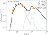 |
Fig. A.1. SED of W61 7-6 and its derived parameters. The lines and symbols represent the same as in Fig. 5. |
WOH G64 is a well-studied dust-enshrouded RSG with an optically thick dust shell (Ohnaka et al. 2008; Levesque et al. 2009; Beasor & Smith 2022). It lacks a spherically symmetric shell, but has a dust torus. This was modelled by Ohnaka et al. (2008), who inferred a luminosity of log(L/L⊙) = 5.45. Integrating the SED would overestimate its luminosity because of the asymmetric shell. The grid of optical depths we used in this case was in the range of [14, 26] μm. In Fig. A.2, we present the best-fit models of WOH G64 with two different assumptions for the grain size: a = 0.3 μm following Beasor & Smith (2022) and the MRN distribution with 0.01 ≤ a ≤ 0.15 μm, as inferred by Ohnaka et al. (2008). In the first case, the result is similar to that of Beasor & Smith (2022), with a difference in the mass-loss rate that could be attributed to the different photometry and fitting method,  . In the second case, we found a better fit that also reproduces the shape of the IRS spectrum. This means that a smaller grain size is better, and it also results in a higher mass-loss rate,
  . We should mention that the WISE photometry is not consistent with the rest of the SED because the source is brighter than the instrument saturation limits. However, it passes the quality criteria we defined in Section 2.
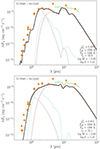 |
Fig. A.2. Two DUSTY SED models of WOH G64 with different grain size assumptions. The lines and symbols represent the same as in Fig. 5. Top: Grain size with a = 0.3 μm. Bottom: MRN distribution with 0.01 ≤ a ≤ 0.15 μm. |
Appendix B: Mass-loss rate relations for radiatively driven winds and different grain size distribution
The best-fit parameters of each wind and grain size assumption are presented in Table B.1. We show the derived Ṁ(L,Teff) relations in Fig. B.1, B.2, and B.3 for RDW and an MRN grain size distribution [0.1, 1] μm, steady-state winds and MRN grain size distribution [0.01, 1] μm, and RDW and MRN grain size distribution [0.01, 1] μm, respectively.
 |
Fig. B.3. Same as Fig. 12 (left), but for RDW and an MRN grain size distribution in the range [0.01, 1] μm. |
Best-fit parameters of Eq. (7) for RDW, steady-state winds with a smaller grain size and only single RSGs.
Appendix C: Binary candidate RSGs
We removed the binary candidates and fitted Eq. (7) in the new sample. We demonstrate the new relation of the probable single RSGs with green points in Fig. C.1. The magenta points show the same relation as in Fig. 12. The two relations differ marginally and mainly in the change of the slope at high L because a significant fraction of binary candidates occupies the lower Ṁ part at high L, as shown in Fig. 11. If these sources are indeed binaries, then we estimated the mass-loss rates under uncertain assumptions, such as the spherical symmetry of the dust shell and the luminosity of the star. We present the best-fit parameters of Eq. (7) for the probably single RSGs in Table B.1.
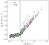 |
Fig. C.1. Derived Ṁ(L,Teff) from the complete RSG sample (magenta), as in Fig. 12, and from the single RSG sample with U − B > 0.7 mag (green). Both relations were applied to the single RSG sample for a one-to-one comparison. |
All Tables
Best-fit parameters of Eq. (7) for RDW, steady-state winds with a smaller grain size and only single RSGs.
All Figures
|
Fig. 1. Colour-magnitude diagram (CMD) of the RSGs in the LMC using 2MASS photometric data. The dashed lines define the photometric RSG limits from Yang et al. (2021), modified by increasing the slope of the right diagonal line. The orange points show the sources we kept in our final sample. |
| In the text | |
|
Fig. 2. Proper motions in Dec and RA (left) and distribution of parallaxes (right). The blue points show the initial RSG sample, and the orange points show the LMC members after applying the probability criteria from Jiménez-Arranz et al. (2023) with PLMC > 0.26. The grey points indicate sources without a probability measurement from Jiménez-Arranz et al. (2023). Sources located right of the dotted vertical line were considered to be foreground. |
| In the text | |
|
Fig. 3. Spatial distribution of the final RSG sample in the LMC (orange points). The background targets (grey) are the complete sample of all sources from Yang et al. (2021). |
| In the text | |
|
Fig. 4. Luminosity distribution of the RSG candidate sample. |
| In the text | |
|
Fig. 5. Examples of SED fits of two optically thin (top row), two dusty (middle), and two peculiar (bottom row) RSGs. The orange diamonds show the observations, and the black line is the best-fit model consisting of the attenuated flux (dashed light blue), the scattered flux (dot-dashed grey) and dust emission (dotted brown). The green curve represents the Spitzer IRS spectrum. The coordinates of each source are shown in the top left corner. |
| In the text | |
|
Fig. 6. Distributions of SED fitting parameters. Left: distribution of the minimum |
| In the text | |
|
Fig. 7. Distribution of the best-fit effective temperatures from DUSTY. The lines show the applied J − Ks empirical prescriptions from Neugent et al. (2012) (orange) and Britavskiy et al. (2019) (dashed black) to our sample. |
| In the text | |
|
Fig. 8. Derived mass-loss rate as a function of the luminosity of each RSG candidate in the LMC. The colour bar shows the best-fit τV. The grey triangles represent the upper limits of targets fitted with the lowest values of the optical depth grid, and the open circles indicate the RSGs with spectral classifications. The dust-enshrouded RSG, WOH G64, is labelled with a red star. The position of the kink is shown with a dashed vertical line at log(L/L⊙) = 4.42. |
| In the text | |
|
Fig. 9. MAD of W1 band vs. luminosity diagram. The colour bar shows the corresponding mass-loss rate of each source. The open circles indicate the RSGs with spectral classifications, and the dashed line represents the position of the kink, as in Fig. 8. |
| In the text | |
|
Fig. 10. Colour-colour diagram of U − B and B − V. The blue points show all sources with UBV photometry. The orange circles indicate RSGs from Neugent et al. (2020) with a probability of an OB companion Pbin > 0.6. The vertical dotted line corresponds to the limit applied to separate probable binary from single RSG. |
| In the text | |
|
Fig. 11. Same as Fig. 8, but for log(L/L⊙) > 4, indicating the binary candidates (U − B < 0.7 mag) with orange circles. |
| In the text | |
|
Fig. 12. Mass-loss rates vs. luminosity (left) and effective temperature (right) calculated from Eq. (1). The magenta points correspond to the prediction of the derived Ṁ(L,Teff) relation, Eq. (7), showing the correlation of the mass-loss rate as a function of the luminosity and effective temperature. |
| In the text | |
|
Fig. 13. Comparison between the resulting mass-loss rates of steady-state winds and RDW. Top: mass-loss rate vs. luminosity. The results from steady-state winds and RDW are indicated with blue and orange, respectively. The solid line shows the relation by Yang et al. (2023) in the SMC corrected by adding 0.7 dex. Bottom: the ratio of the results of the two modes. |
| In the text | |
|
Fig. 14. Effect of the grain size distribution on the mass-loss rate for a range of luminosities. Top: ratio of the mass-loss rates assuming an MRN grain size distribution in the range [0.01, 1] μm over the distribution in the range [0.1, 1] μm. Bottom: ratio of the minimum |
| In the text | |
|
Fig. 15. Comparison of our Ṁ(L) result (open circles) with prescriptions from previous works presented in Table 4. The two lines from Beasor et al. (2020) correspond to an initial mass of 10 M⊙ and 20 M⊙, and the same holds for Kee et al. (2021), but represents the current mass. |
| In the text | |
|
Fig. A.1. SED of W61 7-6 and its derived parameters. The lines and symbols represent the same as in Fig. 5. |
| In the text | |
|
Fig. A.2. Two DUSTY SED models of WOH G64 with different grain size assumptions. The lines and symbols represent the same as in Fig. 5. Top: Grain size with a = 0.3 μm. Bottom: MRN distribution with 0.01 ≤ a ≤ 0.15 μm. |
| In the text | |
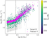 |
Fig. B.1. Same as Fig. 12 (left), but for RDW. |
| In the text | |
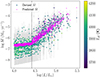 |
Fig. B.2. Same as Fig. 12 (left), but for an MRN grain size distribution in the range [0.01, 1] μm. |
| In the text | |
|
Fig. B.3. Same as Fig. 12 (left), but for RDW and an MRN grain size distribution in the range [0.01, 1] μm. |
| In the text | |
|
Fig. C.1. Derived Ṁ(L,Teff) from the complete RSG sample (magenta), as in Fig. 12, and from the single RSG sample with U − B > 0.7 mag (green). Both relations were applied to the single RSG sample for a one-to-one comparison. |
| In the text | |
Current usage metrics show cumulative count of Article Views (full-text article views including HTML views, PDF and ePub downloads, according to the available data) and Abstracts Views on Vision4Press platform.
Data correspond to usage on the plateform after 2015. The current usage metrics is available 48-96 hours after online publication and is updated daily on week days.
Initial download of the metrics may take a while.