Investigating episodic mass loss in evolved massive stars

S. de Wit; A. Z. Bonanos; K. Antoniadis; E. Zapartas; A. Ruiz; N. Britavskiy; E. Christodoulou; K. De; G. Maravelias; G. Munoz-Sanchez; A. Tsopela

doi:10.1051/0004-6361/202449607

Home

All issues

Volume 689 (September 2024)

A&A, 689 (2024) A46

Full HTML

Open Access

Issue		A&A Volume 689, September 2024


Article Number		A46
Number of page(s)		22
Section		Stellar atmospheres
DOI		https://doi.org/10.1051/0004-6361/202449607
Published online		02 September 2024

A&A, 689, A46 (2024)

II. Physical properties of red supergiants at subsolar metallicity^★

S. de Wit¹^,2^,**, A. Z. Bonanos¹, K. Antoniadis¹^,2, E. Zapartas³^,1, A. Ruiz¹, N. Britavskiy⁴^,5, E. Christodoulou¹^,2, K. De⁶, G. Maravelias¹^,3, G. Munoz-Sanchez¹^,2 and A. Tsopela⁷

¹ IAASARS, National Observatory of Athens, Metaxa & Vas. Pavlou St., 15326 Penteli, Greece
² National and Kapodistrian University of Athens, Department of Physics, Panepistimiopolis, 15784 Zografos, Greece
³ Institute of Astrophysics FORTH, 71110 Heraklion, Greece
⁴ University of Liège, Allée du 6 Août 19c (B5C), 4000 Sart Tilman, Liège, Belgium
⁵ Royal Observatory of Belgium, Avenue Circulaire/Ringlaan 3, 1180 Brussels, Belgium
⁶ Kavli Institute for Astrophysics and Space Research, Massachusetts Institute of Technology, Cambridge, MA, USA
⁷ Department of Physics and Astronomy, Dartmouth College, 6127 Wilder Laboratory, Hanover, NH 03755, USA

Received: 14 February 2024
Accepted: 2 April 2024

Abstract

Mass loss during the red supergiant (RSG) phase plays a crucial role in the evolution of an intermediate-mass star; however, the underlying mechanism remains unknown. We aim to increase the sample of well-characterized RSGs at subsolar metallicity by deriving the physical properties of 127 RSGs in nine nearby southern galaxies. For each RSG, we provide spectral types and used MARCS atmospheric models to measure stellar properties from their optical spectra, such as the effective temperature, extinction, and radial velocity. By fitting the spectral energy distribution, we obtained the stellar luminosity and radius for 92 RSGs, finding that ~50% of them have log(L/L_⊙) ≥ 5.0 and six RSGs have R ≳ 1400 R_⊙. We also find a correlation between the stellar luminosity and mid-IR excess of 33 dusty variable sources. Three of these dusty RSGs have luminosities exceeding the revised Humphreys-Davidson limit. We then derived a metallicity-dependent J − K_s color versus temperature relation from synthetic photometry and two new empirical J − K_s color versus temperature relations calibrated on literature TiO and J-band temperatures. To scale our derived cool TiO temperatures to values that are in agreement with the evolutionary tracks, we derived two linear scaling relations calibrated on J-band and i-band temperatures. We find that the TiO temperatures are more discrepant as a function of the mass-loss rate, and discuss future prospects of the TiO bands as a mass-loss probe. Finally, we speculate that three hot dusty RSGs may have experienced a recent mass ejection (12% of the K-type sample) and classify them as candidate Levesque-Massey variables.

Key words: stars: atmospheres / stars: fundamental parameters / stars: late-type / stars: massive / stars: mass-loss / supergiants

^★

Based on observations collected at the European Southern Observatory under ESO programs 105.20HJ and 109.22W2.

^**

Corresponding author; e-mail: sdewit@noa.gr

© The Authors 2024

Open Access article, published by EDP Sciences, under the terms of the Creative Commons Attribution License (https://creativecommons.org/licenses/by/4.0), which permits unrestricted use, distribution, and reproduction in any medium, provided the original work is properly cited.

This article is published in open access under the Subscribe to Open model. Subscribe to A&A to support open access publication.

1 Introduction

Massive stars contribute significantly to the evolution of galaxies by providing mechanical feedback and chemically enriching the interstellar medium. It is therefore crucial to understand their evolution and feedback mechanism, specifically those channeled through stellar winds and outbursts, which can significantly alter the late-stage evolution of a massive star, as well as the properties of the resulting supernova and compact remnant (Smith 2014). Mass loss during red supergiant (RSG) phase (Levesque 2017; Decin 2021) is a significant contributor to these channels, as the majority of massive stars either evolve through this phase (either transitioning into yellow supergiants or yellow hypergiants; e.g., de Jager 1998; Gordon & Humphreys 2019) or terminate their lives as a RSG via a core-collapse supernova or a direct implosion into a black hole (Heger et al. 2003; Sukhbold et al. 2016; Laplace et al. 2020). Stars lose mass at higher rates in the RSG phase compared to the OB main-sequence phase (by ~1 order of magnitude, depending on the metallicity; Beasor et al. 2021), but there are still many uncertainties regarding RSG outflows, on both theoretical and empirical grounds (see, e.g., Antoniadis et al. 2024). Additionally, there are clues regarding the episodic mass loss in these complex stellar outflows (Smith 2014; Bruch et al. 2021; Humphreys & Jones 2022).

The mass-loss behavior of RSGs, although significant, remains elusive despite many recent efforts to study the mass-loss rates and driving mechanisms both observationally and theoretically (e.g., Beasor et al. 2020; Kee et al. 2021; Davies & Plez 2021; Decin et al. 2024). Kee et al. (2021) suggest that turbulent motions provide the force to steadily drive material off the stellar surface, and as such the escape mechanism likely does not depend on the radiation field (although this was recently challenged by Vink & Sabhahit 2023). The proposed mass-loss mechanism(s) should be time-dependent, yet we often adopt instantaneous mass-loss rates (de Jager et al. 1988; van Loon et al. 2005; Goldman et al. 2017; Beasor et al. 2020; Yang et al. 2023; Antoniadis et al. 2024) to characterize mass loss throughout the RSG phase. Massey et al. (2023), on the other hand, used the luminosity function to study the role of a time-averaged mass-loss rate.

Empirical prescriptions may differ by two to three orders of magnitude (e.g., de Jager et al. 1988 versus Goldman et al. 2017). Adopting one over another can drastically impact the post-main-sequence evolution in stellar evolution models (e.g., MESA; Paxton et al. 2011, 2013, 2015, 2018): the hydrogen-rich envelope may be stripped, which then affects the supernova type and compact remnant properties after core-collapse (Laplace et al. 2020, 2021). Some empirical prescriptions (Kee et al. 2021; Yang et al. 2023) consistently strip RSG envelopes down to M_ini ~ 15M_⊙ (Zapartas et al., in prep.), while others fail to do so (Beasor et al. 2020; Decin et al. 2024), in conflict with observations (i.e., the lack of exploding RSGs of M_ini ≥ 20 M_⊙, i.e., the “RSG problem”; see, e.g., Smartt et al. 2009; Davies & Beasor 2020; Beasor et al. 2021, or the existence of post-RSG objects, such as “F15” in Decin et al. 2024). Therefore, such observations are typically explained by interactions in binary systems (Eldridge et al. 2013; Zapartas et al. 2017) or short-lived pre-supernova explosions (Smith et al. 2009).

Adding to the complexity of the stellar wind is the variety of assumptions used when deriving $\dot{M}$ $\[\dot{M}\]$ (e.g., the gas-to-dust ratio, geometrical symmetries, the dust composition, and the grain size distribution), as well as uncertainties on the surface properties forming at the base of the wind. An accurately constrained RSG effective temperature (T_eff) is specifically important for spectral energy distribution (SED) fitting models to obtain mass-loss rates (e.g., DUSTY; Ivezic & Elitzur 1997). Furthermore, T_eff is a direct input into several common mass-loss prescriptions (e.g., de Jager et al. 1988; Nieuwenhuijzen & de Jager 1990; van Loon et al. 2005). Not only does T_eff strongly depend on the metallicity, it is also variable due to intrinsic velocity cycles (hysteresis loops; Kravchenko et al. 2019, 2021). Moreover, changes in the immediate circumstellar environment due to a high mass loss (log( $\dot{M}$ $\[\dot{M}\]$ ) ≤ −5.0 dex; Davies & Plez 2021) may significantly hinder the derivation of T_eff. Both the hysteresis loops and mass loss change the appearance of the emerging spectrum, as the location of the photosphere moves inward or outward (see, e.g., Massey et al. 2007; Levesque et al. 2007). To understand stellar outflows, it is crucial to understand the evolutionary state of the RSG, for example T_eff and L_*, which yield a location in the Hertzsprung-Russell diagram (HRD), and the force required to lift material off the surface (e.g., the escape velocity, υ_esc, from the surface gravity, log g, and the turbulent velocity, υ_turb). Not only do spectral properties of RSGs change, but it has been established that RSGs are photometric semi-regular variables, varying by up to a few magnitudes in the optical (Kiss et al. 2006). Luminous RSGs even display significant variability in their infrared (IR) magnitudes (e.g., WISE; Yang et al. 2018).

There are many different methods for obtaining the surface properties of RSGs depending on the wavelength domain in which they were observed. Nearby RSGs, such as Betelgeuse, are resolved and allow for the extraction of complex surface characteristics, such as velocity variations and shifting temperatures at the stellar surface (either due to rapid rotation or convective motions; Kervella et al. 2018; Ma et al. 2024). For extragalactic RSGs, many studies targeted nearby galaxies in the Local Group (i.e., LMC, SMC, NGC 6822, WLM, and Sextans A), but also up to 2 Mpc away (i.e., NGC 300 and NGC 55) with spectroscopy, spanning a range of metallicities, to obtain the effective temperature: Levesque et al. (2005, 2006) fitted titanium-oxide (TiO) molecules in the optical, Davies et al. (2013) fitted the line-free IR continuum, Patrick et al. (2015, 2017) and Gazak et al. (2015) fitted spectral lines in the J band, Tabernero et al. (2018) fitted spectral lines in the i band, and González-Torà et al. (2021) fitted absorption-free spectral windows throughout the whole SED. Most of the methods applied in these studies led to temperatures that are in disagreement with one another. This is likely explained by the stellar atmosphere models used, which are typically 1D (e.g., MARCS; Gustafsson et al. 2008) despite the atmospheres of RSGs having a much more complex 3D structure and motions (e.g., convection and granulation; see Freytag et al. 2002; Ludwig et al. 2009; Chiavassa et al. 2011).

The temperatures obtained through the TiO diagnostic are the main outliers (Davies et al. 2013) as they systematically yield a lower T_eff for a given RSG. This discrepancy has been attributed to increased molecular absorption in the MARCS models, potentially due to a combination of two effects. Firstly, the 1D assumptions in the MARCS models do not precisely represent a 3D RSG atmosphere (Davies et al. 2013), specifically regarding the temperature gradient in the stellar atmosphere. Secondly, the MARCS models ignore the effects of mass loss on the spectral appearance (Davies & Plez 2021), which significantly alters the TiO opacity. Furthermore, Davies et al. (2013) demonstrated that the A_V values derived from TiO-dominated spectra are too low compared to existing extinction maps and the strengths of diffuse interstellar bands of the same spectrum. As such, these authors urged caution when interpreting T_eff and A_V values derived from the TiO diagnostic. However, spectroscopic observations are typically obtained in the optical due to the wide availability of optical spectrographs, particularly for multi-object spectroscopy. Therefore, there is an increasing need for a new T_eff scaling relation to convert between TiO temperatures and the more reliable J-band or i-band temperatures.

A large catalog of RSGs beyond the Local Group, resulting from optical spectroscopy, has recently been presented by the ASSESS¹ project with the aim to study the role of episodic mass loss in evolved massive stars (Bonanos et al. 2024). The next step is to characterize the physical properties of these 127 RSGs with spectral modeling. In Sec. 2 we briefly summarize the observations and target selection, provide an updated spectral classification for each RSG, obtain a stellar luminosity for most RSGs from SED fitting, and present RSG light curves from various surveys. In Sec. 3 we present the spectral modeling strategy and the grid of evolutionary models used in this work. In Sec. 4 we present the stellar properties of our sample of RSGs and derive scaling relations to reinterpret the effective temperatures obtained in this work. We discuss our results in Sec. 5 and summarize them in Sec. 6.

2 Data

2.1 Target selection and observations

Bonanos et al. (2024) presented 129 RSGs located in nine southern galaxies up to 5 Mpc, which were selected primarily by their mid-IR magnitudes and colors. In Table 1, we list the targeted galaxies ordered by right ascension (RA), and their properties such as distance, metallicity, radial velocity, and the number of M-type and K-type RSGs. For 117 of these, no matches were found with spectroscopically classified objects in the literature and were therefore viewed as new discoveries. The other 12 RSGs have counterparts in the literature (five were identified as RSGs in Gazak et al. 2015, six were identified as RSGs in Patrick et al. 2017, and one was classified as G2 I in Evans et al. 2007). Bonanos et al. (2024) imposed strict criteria on the IRAC [3.6] and [4.5] photometric bands, to select dusty, evolved massive stars. These bands were chosen to estimate the amount of IR excess (i.e., due to a hot dust-rich component), which may indicate past episodes of enhanced mass loss.

Here, we break down the criteria as follows: (i) M_3.6 ≤ −9.0 mag; to avoid contamination from the asymptotic giant branch stars (Yang et al. 2020), (ii) m_4.5 ≤ 15.5 mag; to avoid contamination by background galaxies (Williams et al. 2015), and (iii) m₃₆ − m_4.5 > 0.1 mag; to avoid contamination by foreground stars. When a source passed all of these criteria, it was observed as a priority target (f_prio ~ 26%), increasing in priority as the IR excess increased (P1; m_3.6 − m_4.5 > 0.5 mag). A source was observed as a non-priority target (“filler”) if it satisfied none of these criteria. For the RSG sample, 79% are fillers and the vast majority of these do not show IR excess.

We show the location of our RSGs in the Spitzer color–magnitude diagram in the left panel of Fig. 1. Dusty sources with IR excess (m_3.6 − m_4.5 > 0.1 mag) are shown in the right panel of Fig. 1. We note that the IR excess is not necessarily explained by dust and may also arise from molecular emission of SiO and CO bands in the mid-IR (Verhoelst et al. 2009; Davies & Plez 2021) by a RSG with a high mass-loss rate. Contrarily, some of the blue RSGs in Fig. 1 (m_3.6 − m_4.5 < −0.5 mag) may be dusty due to polycyclic aromatic hydrocarbon emission around ~3.3 μm, as speculated in Yang et al. (2018). To convert the apparent magnitudes for each source to an absolute magnitude, we used the distances from Table 1. The target IDs, coordinates, magnitudes, spectral types (see Sec. 2.2), variability properties, and light curves (see Sec. 2.4) are presented in Table 2. This table contains identical data to those presented in Bonanos et al. (2024), except for the Gaia Data Release (DR) 2 magnitudes, which were replaced with Gaia DR3 magnitudes (Table 2), and the updated distances to the galaxies in Table 1.

Following our target selection strategy, apart from the RSGs studied here, we observed a wide variety of evolved massive stars, such as luminous blue variable candidates, yellow super-giants, and supergiant B[e] stars, and provided an initial classification in both Bonanos et al. (2024) and Maravelias et al. (2023). The spectra were taken by the Very Large Telescope using the multi-object spectroscopy mode of the Focal Reducer and Low Dispersion Spectrograph (FORS2) under ESO programs 105.20HJ and 109.22W2. The observing details, grism choice, and reduction process were presented in Bonanos et al. (2024). The resulting spectra yielded a resolving power of R ~1000 and provided a wavelength coverage from ~5300–8450 Å. A direct determination of the luminosity class was not possible, as the Ca II triplet (~8500–8700 Å) was not covered.

Table 1

Properties of the galaxies studied in this work.

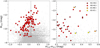Fig. 1

Color magnitude diagrams of 129 studies RSGs. Left: [3.6]-[4.5] versus M_[36]. Gray background points are sources from the Spitzer point source catalog of NGC 300. The dashed lines indicate the region of prioritized sources described in Bonanos et al. (2024) and show some degree of IR excess. Right: zoomed-in view of 34 prioritized dusty targets (33 classified). Red to yellow colors indicate a shift in spectral type toward hotter RSGs. The gray circle indicates the unclassified RSG. Four dusty K-type RSGs are highlighted: NGC3109-167 (1), NGC55-244 (2), NGC55-202 (3), and M83-682 (4).

Table 2

Photometric properties of our RSG sample (extract).

2.2 Spectral classification

The RSGs presented in Bonanos et al. (2024) were initially broadly classified into spectral class K or M. Here, we revisited the spectra and assigned an approximate spectral type (e.g., K0-K5, K5-M0, M0-M2, and M2-M4). It was not possible to determine the exact spectral type, due to the low spectral resolving power, low signal-to-noise ratio, or missing diagnostics (i.e., the Ca II triplet and, in nine cases, both sets of Na II and K I lines). When the TiO bands were either weak or completely absent, we assigned a K0-K5 spectral type. If the TiO bands at λλ6150 and λλ7050 were somewhat present, we assigned a K5-M0 spectral type. We assigned a spectral type M0-M2 to spectra displaying moderately strong λλ6150 and λλ7050 bands, but no molecular TiO absorption at λλ7600. Finally, if all TiO bands were strong, and the spectrum showed significant TiO absorption at λλ7600, we assigned an M2-M4 spectral type. We were unable to determine a spectral type for two RSGs (NGC300-237 and NGC300-609), due to spectral reduction artifacts. The revised spectral types of the RSGs are listed under “Spectral class” in Table 2.

Despite the spectra showing only features of single RSGs, we cannot exclude two possible groups of contaminants. Firstly, given their intrinsic brightness and similarity in spectral features, luminous extragalactic oxygen-rich asymptotic giant branch stars may contaminate our sample (although extremely rare, they can reach up to log (L/L_⊙) ~ 5.0; Groenewegen & Sloan 2018). Secondly, especially for more distant galaxies, the observed spectrum may be a composite of a RSG with other stars (due to multiplicity or an unresolved small cluster), which do not significantly contribute to the optical spectrum, and therefore the temperature diagnostics in the spectrum remain unchanged. It may however affect the photometry presented in Fig. 1 and Table 2, which in turn could lead to overestimated luminosities.

We show the distribution of spectral types in Fig. 2, distinguishing between RSGs with and without IR excess. For the sample with IR excess (hereafter, the “dusty sample”), we considered stars satisfying the first and third criteria presented in Sec. 2.1, to be consistent with Bonanos et al. (2024). Typically, RSG atmospheric models have m_3.6 − m_4.5 ranging from −0.3 to −0.15 from synthetic photometry. The selected limit of an IR excess ≥ 0.1 mag is therefore conservative. We indicate spectral types of the dusty sample in the right panel of Fig. 1. Although most dusty RSGs are late types (i.e., more evolved), we classified a few very dusty RSGs as K types (see Sec. 5.2 for a discussion).

2.3 SED luminosities

We collected photometry from Gaia DR3 (Gaia Collaboration 2023), SkyMapper DR2 (Onken et al. 2019), Pan-STARRS1 (Chambers et al. 2016), 2MASS (Cutri et al. 2003), VISTA Hemisphere Survey (McMahon 2012), and Spitzer IRAC bands (Fazio et al. 2004; Rieke et al. 2004). We presented these magnitudes for each source in Table 2. We used these magnitudes to construct the SED for each RSG. We examined each SED individually and discarded bad photometric points when they were significantly contaminated by excess flux from another source (e.g., due to a low instrumental spatial resolution). For 92 targets with sufficient photometric data in the optical, near-IR, and mid-IR, we calculated the luminosities using one of three methods: (i) when at least one optical band in addition to Gaia bands (e.g., Pan-STARRS1 or SkyMapper r, i, or z), at least one near-IR band (J, H, or K_s) and [3.6] to [8.0] were available, we integrated the observed SED, resulting in a fully data-driven stellar luminosity. However, when these criteria were met (34), in most cases the optical and near-IR were fully sampled (all grizy, G_bp, G, G_rp, or JHK_S were available for a more concise integration). Secondly, (ii) when one wavelength regime was fully unconstrained (i.e., either grizy or JHK_S was fully missing), we fitted a Planck function to the photometric points and obtained the luminosity by integrating the Planck function. Finally, (iii) when a K_S-band magnitude was available, we used bolometric corrections from Davies et al. (2018, BC_K = 2.69 ± 0.11 mag for K-type stars and BC_k = 2.81 ± 0.07 mag for M-type stars) to obtain the absolute magnitude and subsequently, the luminosity.

Given that RSG fluxes peak in the near-IR, integrating the observed SED (first method) underestimates the luminosity in cases where near-IR photometry was unavailable. Furthermore, the third method was not applicable in most cases, given the lack of K_S-band photometry and the increased likelihood of contamination to the K_S-band magnitude for more distant sources. Ultimately, we derived the luminosities of 92 RSGs using the second method. We find that 45 RSGs have a luminosity above log(L/L_⊙) = 5.0. We used the first and third methods on 34 and 73 RSGs, respectively, to verify a general agreement among these three methods within error bars. Examples of SED fits with a Planck function are shown in Fig. A.1 (see Sects. 5.1 and 5.2 for a further discussion on these objects). We corrected the magnitudes for the Galactic foreground extinction from Schlafly & Finkbeiner (2011)². We did not correct for extinction inside the host galaxy, and therefore the intrinsic luminosities may be higher as a small fraction of the emitted light is scattered by interstellar dust. In the case of circumstellar dust, the flux escapes as IR excess. We did not explicitly fit the excess bump from 3.6–24 μm, although its contribution to the total luminosity is negligible in most cases. When significant, the overall Planck curve was lifted to higher fluxes as a result of χ² minimization, and the area under the curve, yielding the luminosity, increased. We also note that in distant galaxies, despite discarding bad photometry, the mid-IR photometry occasionally still appeared slightly contaminated. The mid-IR fluxes, however, only have a minor contribution to the total luminosity of the RSG. The luminosities are presented in the penultimate column of Table 3. The uncertainty in the luminosity was obtained by propagating the magnitude and distance uncertainty of each galaxy, both of which are small. The other columns of Table 3 contain the properties derived from spectral fitting and are described in Sect. 4.1.

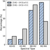Fig. 2

Distribution of spectral types of classified RSGs. Blue hatched bars show RSGs with IR excess (see the right panel of Fig. 1; 33 targets). The remaining RSGs (94) are shown with gray bars.

2.4 Light curves

2.4.1 Optical light curves

Red supergiants can vary by up to two magnitudes in the optical, particularly if they are very evolved and luminous (Kiss et al. 2006; Yang & Jiang 2011, 2012). We therefore searched the Pan-STARRS, Gaia, and ATLAS (Tonry et al. 2018) surveys for multi-epoch photometry of our targets to construct light curves and study them for variability. Due to the faintness of our targets, we were only able to obtain optical light curves for 7 targets from ATLAS, 21 targets from Pan-STARRS DR2, and 4 targets from Gaia DR3. We found ATLAS light curves in both the ATLAS-c and ATLAS-o bands for NGC55-40, NGC55-75, NGC55-135, NGC55-165, NGC300-263, NGC300-154, and NGC3109-167 (see the last column of Table 2), with hundreds of data points covering ~7.5 yr. However, the error bars on the data were too large to indicate any variability from the light curves.

From Pan-STARRS DR2, we found multi-epoch photometry for 21 targets in 5 galaxies (the other 4 galaxies were too far south to be covered by Pan-STARRS DR2), with at least two measurements in one band with an uncertainty below 0.1 mag (see Fig. A.2 for all Pan-STARRS DR2 light curves). We computed the amplitude of the light curve by taking the difference between the minimum and maximum values. The last column of Table 2 lists the photometric bands for which these targets have two or more measurements. Only four targets (NGC3109-167, SextansA-1906, NGC247-154, NGC253-872), have coverage in all grizy bands. Here, we highlight five interesting cases with an amplitude greater than 1 mag. NGC253-222 has Δi,z, and y of ~1.8 mag, ~1.4 mag, and ~2.5 mag, respectively, NGC253-872 has Δr of ~1.4 mag, NGC253-1534 has Δi of ~2.1 mag, NGC247-447 has Δi of ~1.0 mag and NGC247-154 has Δr, i of ~1.4 mag and ~1.0 mag, respectively. Each of these five RSGs was classified as an M-type RSG, with three of them showing IR excess.

For four targets (NGC300-59, NGC300-125, NGC247-3683, and NGC253-872), we constructed light curves from Gaia DR3, containing 70 data points spanning ~ 3 years. For these sources, we reported a min-max ΔG of ~1.5, ~0.9, ~0.6, and ~0.6 mag, respectively. We show the Gaia DR3 light curve of NGC300-59 in the top panel of Fig. 3 (see Fig. A.3 for the other three light curves. The stellar luminosity for this source was log(L/L_⊙) = 5.21. NGC300-59 was particularly interesting as it additionally varied significantly in the mid-IR (see Sect. 2.4.2). The observed long period of ~ 1000 days (min to max ~500 days) is reasonable compared to the periods found for other bright RSGs (Yang & Jiang 2011, 2012).

Recently, Riello et al. (2021) developed a method for inferring the variability of Gaia sources for which a light curve is not available. This method hinges on the fact that magnitudes have a typical, expected uncertainty corresponding to their brightness. When a RSG has a higher G-band uncertainty than expected for a given brightness, it is likely due to fluctuating measurements (due to, e.g., intrinsic variability). For 93 RSGs in our sample containing Gaia G-band measurements, we tested whether they are above the threshold indicated in Fig. 14 of Riello et al. (2021). We find 38 RSGs above this threshold, indicating they are “likely” medium-to-high amplitude variables. From the previous eight RSGs highlighted as either Pan-STARRS DR2 or Gaia variables, five (NGC300-59, NGC300-125, NGC247-154, NGC253-872, and NGC253-222) had a Gaia uncertainty above the threshold and one had no Gaia measurements, meaning only two sources were not correctly selected as variables using this method. NGC247-3683 did not exceed the threshold, though it is at the limit, despite showing a 0.5 mag variation in its Gaia G-band light curve.

Table 3

Physical parameters of our RSG sample (extract).

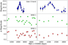Fig. 3

Gaia G-band (top), WISE1 (middle), and WISE2 (bottom) light curves for NGC300-59. A zoomed-in view around the peak of the Gaia measurements is shown on the right.

2.4.2 Mid-IR light curves

If a RSG loses a variable amount of mass with time, it should become apparent in the mid-IR light curve, as the circumstellar dust, on which the photons scatter, forms and dissipates as it propagates. We collected light curves for WISE1 (3.4 μm) and WISE2 (4.6 μm) for NGC 55 and NGC 300 (82 sources), using the difference imaging pipeline for WISE data described in De et al. (2023). Where possible, using these light curves, we studied the connection between the optical and mid-IR variability. All WISE1 light curves contained 20 epochs, spanning ~12.5 years. First, we derived the median absolute deviation (MAD) values for WISE1, to check the relation between variability and luminosity. We present these MAD values as MAD_W1 in Table 2. In Fig. 4, we visualized the sources that are variable in the mid-IR in a MAD diagram, as a function of their magnitude and luminosity. We see that the MAD value generally increased with magnitude, due to the increasing uncertainty on the photometry. For sources with comparable magnitudes, we show that RSGs with higher luminosities (see the color bar in Fig. 4) generally have a higher MAD value, which is in agreement with past studies (see, e.g., Yang et al. 2018; Antoniadis et al. 2024). Similarly, we find that 16 out of 19 dusty RSGs have a higher MAD value compared to the median MAD value of non-dusty RSGs (dashed black curve in Fig. 4).

In Fig. 4, we highlight eight sources that were reported as variable from their optical light curves (see Sect. 2.4.1). All of these RSGs had luminosities above log(L/L_⊙) ~ 5.0. We note NGC300-59 (M2-M4 I), which showed the highest MAD value from its WISE1 light curve and was additionally reported as a high-amplitude optical variable in Gaia DR3. In Fig. 3 we show the correlated WISE1 and WISE2 light curves of this source in the middle and bottom panel, respectively. From the zoomin (right panels of Fig. 3), we find that the WISE1 light curve peaks ~100 days after the peak of the Gaia light curve, although the cadence of the WISE observations prevented us from making a more precise estimate of the delay. We discuss this dusty RSG further in Sec. 5.2.

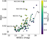Fig. 4

WISE1 versus MAD_wise1 diagram for RSGs in NGC 55 and NGC 300. The color bar indicates the luminosity for each RSG, and the gray dots indicate cases where a luminosity was not obtained. Black stars indicate eight RSGs that were reported as variable in optical surveys. Open circles indicate dusty RSGs. The dashed black curve indicates the median MAD for non-dusty RSGs. Four RSGs with both optical variability and a high MAD value relative to their WISE1 magnitude are labeled.

3 Methodology

3.1 The grid of MARCS models

We constructed a grid of 1D MARCS model atmospheres (Gustafsson et al. 2008) to model for the spectroscopic properties of our RSG sample. Typically, spherical models are used, with a theoretical mass of M_RSG = 15 M_⊙ (see, e.g., Davies et al. 2010, for a discussion on this assumption). Additionally, we adopted the default value for the microturbulent velocity, ξ = 5 km s⁻¹, as González-Torà et al. (2021) show that the fitted effective temperatures are relatively unaffected by ξ (≤ 20 K). Since the targeted galaxies widely varied in metallicity (Z), we adopted a grid of models spanning from log(Z/Z_⊙) = +0.25 to −1.00 dex with Δlog(Z/Z_⊙) = −0.25 dex. We then used linear interpolation, to make the metallicity grid denser to a grid step of Δlog(Z/Z_⊙) = −0.125 dex. Since the TiO molecular bands display a strong degeneracy between T_eff and Z, it was not feasible to derive both parameters from optical spectra. Typically, one resorts to J- or K_S-band spectroscopy to robustly derive a value for Z (e.g., Gazak et al. 2015; Patrick et al. 2015, 2017). Therefore, to lift the degeneracy between T_eff and Z, we fixed the metallicity to the average metallicity reported in the literature for each galaxy (see Table 1). Lastly, we fixed the surface gravity, log g, to +0.0 dex (commonly assumed in, e.g., Carr et al. 2000; Levesque et al. 2005; Davies et al. 2010). We emphasize that the resulting bestfit parameters should not be affected by this choice, given that no spectral features in our wavelength range were sensitive to changes in log g (e.g., the Ca II triplet).

We modeled T_eff, the color excess E(B − V), and υ_rad as free parameters. Through linear interpolation, we constructed a T_eff grid ranging from 3300–1000 K with ΔT_eff = 10 K and from 4000–1500 K with ΔT_eff = 25 K. The changing step size at T_eff ≥ 4000 K was motivated by the decreasing impact of the temperature on the strengths of the TiO band as the temperature increases. Although constraining the temperature down to a 10 K precision was not realistic, given all the physical uncertainties on the RSG temperature (e.g., spectral variability due to hysteresis loops), a dense grid allowed us to constrain the statistical uncertainties to a greater accuracy. To derive E(B − V), and subsequently A_V, we applied Fitzpatrick (1999) extinction laws to the models. We assumed a total-to-selective extinction coefficient of R_V = 3.1 for all galaxies. Although we note that R_V may be different in a circumstellar environment compared to the interstellar medium (Massey et al. 2005), we argue that fixing R_V to this value was acceptable, as González-Torà et al. (2021) demonstrated that the resulting T_eff is barely affected by changes in R_V. We varied E(B − V) between 0.0 and 3.0 magnitudes with a step size of ΔE(B − V) = 0.05 mag.

3.2 Spectral fitting strategy

First, we scaled the spectral properties of the MARCS models to match those of the observed spectra. We downgraded the resolving power of the models to R ~ 1000 (using PYASTRONOMY.INSTRBROADGAUSSFAST), to match the spectral resolution of our FORS2 grism. We then resampled the wavelength grid of the model to make it identical to the grid of the spectrum. To optimize the modeling of the RSG spectra, a similar smoothing tactic was chosen as presented in de Wit et al. (2023). We fitted 15 to 20 selected spectral windows of ~50 Å, containing crucial spectroscopic diagnostics (i.e., the molecular TiO bands to derive T_eff). By selecting bins, regions without diagnostics did not influence the resulting best-fit χ². Moreover, fitting narrow wavelength bins exposed some of the inherent uncertainties in specific rotational and vibrational line transitions of the TiO molecules present in the models. Both of these effects on the best-fit χ² were now minimized as they are smoothed out over a ~50 Å range. The number of bins used per star depended on the range of the observed spectrum. Some spectra missed a TiO band either in the reddest or bluest part (i.e., due to reduction errors, due to the physical position of the slit at the edge of the detector, or due to contamination of blue wavelengths by another source). In a few spectra, some TiO bands were substantially contaminated with strong nebular emission lines from the ambient medium, and as such were excluded from the calculation. We calculated χ² as follows: $χ^{2} = \sum_{i}^{n} {(\frac{F_{i} - F_{i, m o d}}{E_{i}})}^{2},$ $\[\chi^2=\sum_i^n\left(\frac{F_i-F_{i, \mathrm{mod}}}{E_i}\right)^2,\]$ (1)

in which n is the amount of bins, F_i is the flux of the spectral bin, F_i_,mod the flux of the model bin and E_i is the uncertainty on the flux in spectral bin i. The model with the lowest χ² was accepted as the best-fit model, and its free parameters were accepted as the best-fit numerical solution.

We iteratively fitted the entire RSG sample using the previously discussed minimum χ² routine. First, we fixed Z and υ_rad to the value of the host galaxy (see Table 1 for details per galaxy). We then fitted the 2D grid of MARCS models to obtain the best-fit T_eff and E(B − V). However, the resulting best-fit parameters marginally depend on the adopted values for υ_rad, especially in galaxies with a strong rotational curve (e.g., NGC 253; see Hlavacek-Larrondo et al. 2011). Therefore, using a cross-correlation technique, we used the best-fit model as an input to derive a more accurate value for υ_rad. Following a similar χ² algorithm, we shifted the model with Δυ_rad = 10 km s⁻¹ to obtain the numerical best-fit velocity shift from the lowest χ². When the best-fit υ_rad differed from the adopted υ_rad of the host galaxy, we updated the input υ_rad and repeated the fitting process until the solution converged. When converged, we verified the numerical results by visually inspecting the best-fit model applied to the spectrum. Similar to de Wit et al. (2023), we constructed a 2D χ² map to derive the 1 to 3σ uncertainties from contours, enclosing the $χ^{2} = χ_{min}^{2} + Δ χ^{2}$ $\[\chi^2=\chi_{\min }^2+\Delta \chi^2\]$ values (where Δχ² = 2.3,6.2, and 11.8 are the values for which the probabilities exceed 1σ-3σ, respectively).

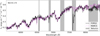Fig. 5

Best-fit MARCS model to NGC55-174, an M0-M2 I star. The FORS2 spectrum is indicated in black, the medium-resolution MARCS model in magenta, and telluric contaminated regions in gray shades.

3.3 The grid of evolutionary models

To compare the results from spectroscopic fitting to evolutionary predictions, we constructed single-star populations of RSGs at different metallicities using the state-of-the-art POSYDON population synthesis framework (Fragos et al. 2023). POSYDON builds on top of MESA models (Paxton et al. 2011, 2013, 2015, 2018). We assume a Kroupa (2001) initial mass function and a constant star formation history, to generate a sample of RSGs. In our population synthesis analysis, those that produce a neutron star as the end product of stellar evolution (~7–30 M_⊙) are considered RSGs.

Although most massive stars are expected to interact with a binary companion (Sana et al. 2012; de Mink et al. 2014), in this first comparison we ignore the possible binary history of RSGs, producing populations based solely on single star tracks. For this, we used the currently developed default POSYDON tracks extending below solar metallicity (Andrews et al., in prep.), at Z = 0.1, 0.2, 0.45, 1.0 Z_⊙. We added one metallicity (Z = 0.3 Z_⊙) to the existing options, as the metallicity of NGC 55 (42 RSGs) is not well represented by Z = 0.2 Z_⊙ nor Z = 0.45 Z_⊙.

Several assumptions in POSYDON are tailored specifically to massive stars. For the convective core overshooting, default assumptions for POSYDON were assumed. The exponential overshooting scheme was used for a more gradual overshooting, albeit calibrated toward the Bonn step overshoot (Brott et al. 2011). No overshooting is assumed for shell burning. The models do not consider rotation (υ_rot = 0 kms⁻¹). The wind scheme incorporated in these models follows the “Dutch” wind recipes (de Jager et al. 1988; Vink et al. 2001, for cool and hot winds, respectively). The mixing length parameter has been fixed to α_MLT = 1.93. This parameter handles the convection physics in the RSG atmosphere and the envelope structure (and subsequently, the stellar radius and effective temperature) is therefore highly dependent on the assumed value (Henyey et al. 1965; Meynet et al. 2015).

To generate a robust enough RSG population, we generate 50k seeds. We can then obtain useful statistics such as the average effective temperature of a population at given metallicity <T_eff> (later incorporated in Sec. 4.1) according to the current evolutionary predictions and assumptions.

4 Results

4.1 Spectroscopic results

We applied the grid of MARCS models to 127 RSG spectra and obtained their physical properties. In most cases we find a good fit (numerically and visually) to these diagnostics: (i) the TiO absorption bands for T_eff, (ii) the slope of the spectrum for E(B − V), and (iii) individual spectral lines such as Ba II λ6496, to verify the computed υ_rad. We demonstrate the quality of a single best-fit model applied to NGC55-174 in Fig. 5 (Fig. A.4 presents all the other fitted spectra). The uncertainties of the parameters from the MARCS model fits were computed using the χ² map presented in Fig. 6, by adopting the 1σ contour as the final uncertainty on T_eff and E(B − V).

We note that the statistical error, resulting from the minimum-χ² analysis, is unrealistically small in some cases (i.e., ±10 K). For these sources, the computed error on the flux is small, and slight deviations between the model flux and observed flux result in high χ² values. A more realistic uncertainty on the effective temperature is at least 50 K, considering intrinsic temperature variations, uncertainties in the spectral reduction process, and statistical uncertainties. Therefore, whenever the uncertainty from the minimum-χ² analysis dropped below this 50 K threshold, we adopted a minimum uncertainty of 50 K (similar to, e.g., Levesque et al. 2006).

In Table 3, we present the ID, quality flags, the best-fit T_eff, best-fit E(B − V), adopted log(Z/Z_⊙), and best-fit υ_rad for 127 RSGs, as well as both the stellar luminosities computed in Sec. 2.3 and the stellar radii of 92 RSGs using the Stefan–Boltzmann relation. We show the radii and luminosities of each RSG in Fig. 7. We find six RSGs with extreme stellar radii (R ≳ 1400 R_⊙; NGC7793-34, NGC300-125, NGC247-154, NGC247-155, NGC253-222, and NGC1313-310), which are discussed further in Sec. 5.2. Their SED-fitted luminosities are shown in Fig. A.1. Each of these SED fits is good by eye (except NGC247-155), although future observations are necessary to show that these are indeed single, uncontaminated RSGs.

For five RSG spectra (NGC55-93, NGC300-125, NGC247-447, NGC247-2706, and NGC253-784), the best-fit model selected by the χ² routine did not provide a good solution. From these five, we fitted only the spectrum of NGC300-125 by eye, as there were better solutions available. We measure T_eff = 3350 K and E(B − V) = 0.4 mag, with a υ_rad of 160 km s⁻¹, adopt conservative uncertainties of 50 K and flag this source in Table 3 (flag = 1). We find a good χ² in the other four cases, yet the best-fit model still fitted unsatisfactorily by eye (flag = 2).

For eight RSG spectra, the flux in the blue wavelengths was contaminated, yielding unreasonable E(B − V) when included in the fit, and subsequently, unreasonable T_eff. For these cases (NGC7793-274, NGC7793-331, NGC55-1861, NGC247-155, NGC247-1825, NGC253-1534, NGC253-222, and NGC253-1226), we discard the blue wavelengths (λ ≤ 6000Å) and fit only wavelengths where the RSG dominates the flux. The derived extinction for these eight sources (flag = 3) should be taken cautiously. For four RSG spectra, the fit was satisfactory (NGC55-447, NGC55-NC2, NGC253-3509, and NGC253-1137), but the uncertainties were extreme due to the low signal-to-noise ratio of the spectra (flag = 4). Finally, for five RSG spectra (NGC55-135, NGC300-59, NGC300-154, NGC300-173, and NGC300-240), the TiO bands were deeper (i.e., cooler) in the red and shallower (i.e., hotter) in the blue compared to the best-fit model (flag = 0). However, the effect on the derived T_eff is small, and these were therefore included in the analysis in Sec. 5.2.

To illustrate how the derived temperatures change with metallicity, we show temperature distributions for different Z in Fig. 8, discarding sources with flags 2–4. The peak and temperature spread of the distribution shifts to hotter temperatures with decreasing metallicity (shown by the increasing number of RSGs at hotter temperatures in the middle and bottom panels of Fig. 8). In the bottom panel, we have eight RSGs with a T_eff ≥ 4000 K, compared to only one RSG in the middle panel. Lower metallicity stars have more compact envelopes due to the decreased opacity; therefore, this shift in average temperature with metallicity is expected (see Elias et al. 1985; Levesque 2017). Table 4 shows the average T_eff and υ_rad for galaxies with N_RSG ≥ 5, as well as the metallicity and sample size. We verified that the average υ_rad values were in agreement with those listed in Table 1.

Davies et al. (2013) showed that the TiO diagnostic produces RSG temperatures that are generally too cool. We compiled the average temperature of various spectroscopic literature studies on RSG using a variety of diagnostics and compared them to our average T_eff in Fig. 9. We present temperatures obtained from SED fits (González-Torà et al. 2021), metallic lines in the J band (Patrick et al. 2015, 2017; Gazak et al. 2015; Davies et al. 2015), TiO bands (Levesque et al. 2005, 2006; Britavskiy et al. 2019a), metallic lines in the i band (Tabernero et al. 2018) and lastly, line-free continuum fits (Davies et al. 2013). Fig. 9 demonstrates that the TiO bands systematically yield lower T_eff, compared to both the predictions from POSYDON population synthesis models (see Sec. 3.3) and other literature studies. We note that Gazak et al. (2015) and Patrick et al. (2017) derived a mean Z from their J-band spectra in NGC 300 and NGC 55, respectively, which slightly differs from the metallicity indicated in the top axis referring to the mean Z of the galaxy listed in Table 1.

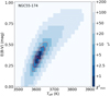Fig. 6

Uncertainties of the best-fit T_eff and E(B − V) of NGC55-174. The red cross indicates the best-fit solution. The blue shades indicate a decrease in the goodness-of-fit, with the 1σ-3σ limits shown with red contours.

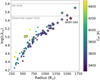Fig. 7

Stellar radius versus luminosity for 92 RSGs. Circles indicate sources from the dusty sample, four of which (including three dusty ones) exceed the revised Humphreys-Davidson limit. Note that the most luminous point contains two overlapping extreme RSGs. WOH G64 is indicated for reference.

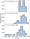Fig. 8

Normalized histogram of the T_eff distribution of our RSG sample for 0.7 Z_⊙ (NGC 253; top), 0.4 Z_⊙ (NGC 300, NGC 247, and NGC 7793; middle), and 0.3 Z_⊙ (NGC 55 and NGC 1313; bottom), excluding sources with flags 2–4.

Table 4

Average parameters of RSGs.

4.2 New color-temperature relations

4.2.1 Empirical T_eff(J-K_S) relations

Color–temperature relations (e.g., T_eff(V − K_S), T_eff(J − K_S); Levesque et al. 2006; Neugent et al. 2012) are often established to estimate the temperature of a population of RSGs from photometry. Such relations require caution, as they are highly influenced by the spectroscopic temperature used for their calibration. Near-IR colors are preferable for such a relation as they are relatively unaffected by extinction and photometric variability, which is much smaller in these bands than in the optical (Schlegel et al. 1998; Whitelock et al. 2003). We proceed to derive new T_eff(J − K_S) relations calibrated on spectroscopic temperatures from the J band and TiO, similar to those derived by Britavskiy et al. (2019a,b) for the Large Magellanic Cloud (LMC) and the Small Magellanic Cloud (SMC), respectively, which were calibrated on the i band.

We combine spectroscopic temperatures of RSGs in the Magellanic Clouds from Levesque et al. (2006) and Davies et al. (2015) to derive new T_eff(J − K_S) relations (see Fig. 10). To derive a relation calibrated on the TiO diagnostics, we used a set of 73 RSG temperatures from Levesque et al. (2006). For the J-band calibrated relation, we used temperatures of 19 RSGs from Davies et al. (2015). We used the A_V coefficient presented in Levesque et al. (2006) and Davies et al. (2013) to correct the J − K_S color for the effect of extinction. We adopted the following color correction Schlegel et al. (1998): (J − K_S)₀ = (J − K_S) − E(J − K) = (J − K_S) − 0.535E(B − V) = (J − K_S) −0.535(A_V/3.1). The values of A_V are systematically lower in Levesque et al. (2006) compared to those derived in Davies et al. (2013), due to the use of the TiO diagnostic, and the intrinsic extinction is likely higher. Therefore, the (J − K_S)₀ colors for this sample (squares in Fig. 10) should be interpreted as upper limits, with the true values likely being lower than derived.

We present the best-fit relations to both sets of RSG temperatures and (J − K_S) colors in both the left panel of Fig. 10 and Table 5. We compare the derived relations to existing empirical relations (Britavskiy et al. 2019a,b) and theoretical relations (Yang et al. 2020; Neugent et al. 2012). The empirical relations are calibrated by using temperatures derived from i-band spectra (Tabernero et al. 2018). The theoretical relations use synthetic photometry from either ATLAS or MARCS models to derive an extinction-free T_eff(J − K_S)₀ relation. We show the literature relations, the diagnostic on which they are calibrated, the metallicity, and the sample size in Table 5. The derived J-band relation agrees with the i-band relation only for LMC metallicity (see Fig. 10), while the TiO relation agrees much more with the theoretical relations, which predict much steeper dependences of T_eff on (J − K_S). We also note that the SMC i-band relation is steeper than its LMC counterpart, suggesting a possible metallicity effect on the slope of the color-temperature relation.

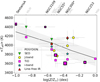Fig. 9

Comparison of our modeled T_eff with the average T_eff of literature studies on RSGs based on the line-free continuum method (red triangles), SED method (green inverted triangles), J-band spectral lines (yellow circles), TiO bands (magenta squares), and i-band spectral lines (cyan stars) in a range of metallicities. TiO results from this work are marked with a thick border; larger squares represent larger sample sizes. The solid black line represents the mean T_eff of a population of RSGs computed with the POSYDON population synthesis code (see Sec. 3.3). The gray shades indicate the standard deviation from the mean T_eff of the RSG population at each metallicity. NGC 300* includes NGC 300, NGC 247, and NGC 7793; NGC 55* includes NGC 55 and NGC 1313.

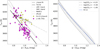Fig. 10

Color-temperature relations at a range of metallicities. Left: new empirical T_eff(J − K_S) relations compared to relations from the literature. Black lines show our new empirical relations based on samples from Levesque et al. (2006, squares) and Davies et al. (2015, circles). Gray lines show the empirical relations from Britavskiy et al. (2019a, LMC i band) and Britavskiy et al. (2019b, SMC i band) and the theoretical relations from Neugent et al. (2012, MARCS) and Yang et al. (2020, atlas). Right: effect of metallicity on the new theoretical T_eff(J − K_S) relations. We demonstrate the relation for the LMC metallicity with a dash-dotted gray line and the fit from Neugent et al. (2012) with a solid blue line. The gray shaded area indicates the effect of metallicity between the most extreme values of our grid (0.1–1.8 Z_⊙).

4.2.2 Theoretical T_eff(J-K_S) relations

To investigate whether the changing slope of the color-temperature relations is expected from theoretical models, we derived new relations using the MARCS atmospheric models for a range of metallicities (0.1 −1.8 Z_⊙). Following the approach of Neugent et al. (2012), we derived a (J − K_S)₀ color for each temperature of the model grid, but for a range of metallicities. We then fit a linear relation to the computed synthetic colors. We find that the slope is relatively unaffected by metallicity (see Fig. 10, right panel), and that there is a small shift toward bluer colors with increasing metallicity. By fitting the differences in offset and slope for each metallicity on the grid, we determine the dependence of the theoretical T_eff(J − K_S) relation on log(Z/Z_⊙). We find a quadratic dependence of the offset (a) and slope (b) and present the relations in Table 5. This new Z-dependent relation can be applied to a wider range of metallicities compared to the Neugent et al. (2012) relation. For LMC metallicity, our relation simplifies to the Neugent et al. (2012) relation.

4.3 TiO scaling relations

Given that the TiO bands produce RSG temperatures that are too cool, it is evident that a direct comparison between the TiO temperatures derived in Sec. 4.1 and for example, evolutionary tracks of RSGs cannot be made. To remedy this, we derive linear scaling relations to shift the TiO temperatures to hotter temperatures and perform such a comparison. We calibrate the TiO temperature scaling relation using a set of reliable near-IR temperatures to minimize systematics. We use 19 RSGs in the SMC and LMC from Davies et al. (2015) and Tabernero et al. (2018) to derive the scaling relation, as each of these objects has a T_eff,TiO, T_eff,J and T_eff,i measurement. This dataset excludes potential differences in spectral reduction or variations in the RSG atmosphere (e.g., hysteresis loops; Kravchenko et al. 2019, 2021), as each of the three temperatures were obtained from the same spectrum and the differences in T_eff arise solely from the different diagnostics. We argue that the i- and J-band diagnostics are reliable to benchmark a scaling relation, as they rely on the modeling of metal lines forming near the stellar continuum region. The line profiles in the MARCS models are well established near the continuum, with major caveats arising mainly at higher altitudes (Davies et al. 2013). Furthermore, deviations from local thermodynamic equilibrium (Bergemann et al. 2012, 2013, 2015) were included in the results of Davies et al. (2015) and Tabernero et al. (2018).

As the data points from Davies et al. (2015) have asymmetric uncertainties, these need to be properly taken into account when performing the linear fit, to not falsely skew the linear relation. Asymmetric uncertainties are specifically strong for high TiO temperatures, due to the nonlinear dependence of the TiO bands on the temperature. The TiO bands significantly increase in strength toward lower atmospheric temperatures, making the upper uncertainty always larger. The most extreme case in our sample has a ~5:1 error ratio.

Each data point has an uncertainty for both variables, which demands complicated regression techniques, for example orthogonal distance regression (ODR; Boggs & Rogers 1990). However, modern implementations of ODR, such as scipy.odr, only treat symmetric uncertainties, while our case demands the treatment of uncorrelated asymmetric uncertainties (Possolo et al. 2019). As a first step to assess our problem, we generate a cloud of points for each of the 19 data points and their uncertainties.

The statistically weighted cloud of points will represent the asymmetric uncertainties. The samples for each point are drawn using the Monte Carlo method. We draw from a statistical distribution, where 1σ represents the uncertainty on the data point reported in the respective studies. For symmetric errors, this distribution simplifies to a Gaussian distribution. However, for the asymmetric cases, we fitted for the shape of the distribution. We obtained a best-fit skewed distribution using a minimization routine, in which the max likelihood of the best-fit posterior represents the value of the data point, and the 1-σ intervals of the best-fit posterior are the asymmetric uncertainties. We then draw 1000 times from the best-fit distribution to generate the final cloud of points.

We used ULTRANEST (Buchner 2021) to perform a linear fit to the clouds of points (19×1000) to find the best underlying relation. ULTRANEST is a Bayesian workflow package that uses nested sampling (Skilling 2004) to obtain a relation between physical properties. We assumed a flat prior and a Gaussian likelihood function, where the mean of the function is given by our two-parameter model (α,β) and a function dispersion, σ. This σ is an additional free parameter that describes the scatter along the initial linear model. The resulting scaling relation is parameterized as follows: $T_{e f f, new} = α + β \times T_{e f f, T i O},$ $\[T_{\mathrm{eff}, \text {new}}=\alpha+\beta \times T_{\mathrm{eff}, \mathrm{TiO}},\]$ (2)

For the J band $α = 3110_{- 610}^{+ 400}, β = {0.24}_{- 0.11}^{+ 0.17}, σ = 58_{- 29}^{+ 21},$ $\[\alpha=3110_{-610}^{+400}, ~\beta=0.24_{-0.11}^{+0.17}, \quad \sigma=58_{-29}^{+21},\]$

and for the i band $α = 2020_{- 750}^{+ 820}, β = {0.49}_{- 0.18}^{+ 0.21}, σ = 15_{- 14}^{+ 31},$ $\[\alpha=2020_{-750}^{+820}, ~\beta=0.49_{-0.18}^{+0.21}, ~~\sigma=15_{-14}^{+31},\]$

where α indicates the offset, β the slope of the relation, and σ the intrinsic Gaussian scatter. We present the best-fit linear relation to the 19 RSG temperatures in Fig. 11. In both panels, we show the calibration temperature on the y-axis. The range for which this relation must be applied is dictated by the T_eff,TiO points from the literature (~3450–3950 K). The shallow slope of the scaling relation suggests that a significant spread in temperatures is not expected for RSGs. Properly sampling the asymmetric uncertainties flattens the best-fit linear relation to the data points compared to doing a simple linear fit (shown in Fig. 11). The deviation of the temperatures from the 1:1 relation implies that, either the diagnostics are not well represented by the 1D atmospheric models, or they are influenced by other stellar properties (e.g., mass loss). The color bar in Fig. 11 reveals that the temperature scales are indeed less discrepant for lower mass-loss rates.

We demonstrate the trend with mass-loss rates in Fig. 12. The mass-loss rates shown for the SMC sources are taken from Yang et al. (2023). For the LMC sources, we obtained mass-loss rates by modeling the circumstellar dust shell around the RSG using the radiative transfer code DUSTY (Ivezic & Elitzur 1997). We assumed a spherically symmetric dust shell, which extends to 10⁴ times the inner radius, and a radiatively driven wind (RDW) as the driving mechanism for mass loss. Antoniadis et al. (2024) discussed caveats in the RDW approach, which, when assumed, lead to overestimated mass-loss rates. However, given that the Yang et al. (2023) results are fixed, we assumed RDW winds for the LMC sources regardless, to allow for a direct comparison between the LMC and SMC supergiants. We adopted the same grain size distribution, grid of models, and fitting methodology as defined in Yang et al. (2023), but adopting a gas-to-dust ratio appropriate for the LMC (r_gd = 380; Roman-Duval et al. 2014) and using MARCS models with [Z] = −0.38. In Fig. 12, the J-band scale is relatively stable with increasing mass-loss rates and shows a large scatter, suggesting that the correlation between the two properties is weak. In contrast, the TiO band scale is more affected and shows a tighter dependence on the mass-loss rate, suggesting they are likely correlated. Using scipy. pearsonr, we find a Pearson coefficient of = −0.89 with a p-value of 2.5 · 10⁻⁷, which suggests a tight statistical anticorrelation between the two variables. This observation agrees with the models shown in Davies & Plez (2021), where a strong stellar wind significantly increases the depths of the TiO bands, while spectral lines in the J band remain unaffected.

For metallicity, we observe a similar effect. Lower metallicity RSGs show a smaller discrepancy between the temperature diagnostics. These RSGs are intrinsically hotter, decreasing the TiO opacity and naturally resolving the discrepancy. Our results strongly suggest that the scaling relation in Eq. (2) should be dependent on both metallicity and mass-loss rate. Future data would not only tighten the uncertainty on the linear relation but would also allow a Z and $\dot{M}$ $\[\dot{M}\]$ dependence to be established. A reliable, all-inclusive scaling relation is particularly useful given that a consistent grid of 3D models or a grid of 1D models, which could self-consistently fit for $\dot{M}$ $\[\dot{M}\]$ has not been established yet (although see Chiavassa et al. 2011, 2022; Davies & Plez 2021; Ahmad et al. 2023, for pioneering sets of models as well as recent developments regarding these models).

Table 5

Overview of the T_eff(J − K_S) relations.

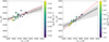Fig. 11

Scaling relations between T_eff,TiO and T_eff,J (left) and between T_eff,TiO and T_eff,i (right). The scattered data points and their uncertainties are taken from Davies et al. (2013, 2015). The thick black line indicates the best-fit scaling relation, the gray shaded band shows the combination of slopes and offsets acceptable within a 1σ uncertainty and the black dotted lines indicate the scatter on the best-fit relation. In red, we show a simple linear fit to the data when one excludes the effect of asymmetric uncertainties. We show a 1:1 relation for comparison. The color bar indicates the mass-loss rates obtained with DUSTY. The sizes of the markers increase proportionally to metallicity.

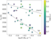Fig. 12

T_eff versus the mass-loss rate for both TiO temperatures (squares; Davies et al. 2013) and J-band temperatures (circles; Davies et al. 2015). Colors indicate the stellar luminosity, and symbol sizes scale with metallicity, as in Fig. 11. A simple linear fit (dashed line) is shown for guidance.

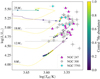Fig. 13

HRD with the observed RSGs in NGC 300 (gray circles), NGC 247 (magenta triangles), and NGC 7793 (cyan squares). Four POSYDON tracks from 8–25 M_⊙ computed for log(Z/Z_⊙) = −0.35 are shown. The color indicates the central helium abundance; the knots on the tracks indicate timesteps of 10 000 yr.

5 Discussion

5.1 HRD analysis

We constructed HRDs and compared our sample to the predictions from pOSYDON evolutionary tracks computed at log(Z/Z_⊙) = −0.35 (0.45 Z_⊙; see Sect. 3.3), to match the metallicities of RSGs in NGC 300, NGC 247, and NGC 7793 (log(Z/Z_⊙) = −0.38). For this metallicity, we obtained both T_eff,_TiO and log(L/L_⊙) for 54 RSGs. We compare these RSGs to the POSYDON tracks in Fig. 13. As expected, the data points are not well reproduced by the tracks, and most RSGs are either located at the final stages of the evolutionary track where the RSG evolves quickly toward central iron exhaustion and subsequent core collapse, or occupy the forbidden zone. Two sources, NGC247-154 at log(L/L_⊙) ~ 5.52 and NGC7793-34 at log(L/L_⊙) ~ 5.58 (see Fig. A.1 for their SED fits), are more luminous than the upper luminosity limit predicted by the evolutionary tracks, even for the core-overshooting properties assumed in POSYDON. Although still well below the classical Humphreys-Davidson limit (log(L/L_⊙) ~ 5.8; Humphreys & Davidson 1979), these two sources have extreme stellar luminosities that exceed the revised Humphreys-Davidson limit (log(L/L_⊙) ~ 5.5; Davies et al. 2018). Their SED-integrated luminosities appear satisfactory; however, an inaccurate distance estimate, reddening estimate, or blending and crowding effects may affect the derived luminosity.

We proceed to apply the new scaling relations (see Sec. 4.3) to 44 out of 54 RSGs shown in Fig. 13 (ten RSGs have temperatures outside the limits of the scaling relations; 3450–3950 K), to test which of the relations shift the observed RSGs to where the tracks are in a steady core-helium-burning phase. The scaled temperatures, using both scaling relations for these RSGs, are compared to the tracks in Fig. 14. The J-band relation scales the RSG temperatures up to values that are too hot compared to the predicted core helium-burning phase of the Hayashi tracks, except at low luminosities. The RSGs are not expected to populate this part of the HRD, as the POSYDON tracks predict a fast Hertzsprung gap crossing for these temperatures. Furthermore, the temperature spread of the J-band-scaled temperatures is narrower than predicted by the models. The i-band-scaled temperatures, however, provide an excellent match with the POSYDON core helium-burning phase, showing a scatter in log(T_eff) compatible with the spread of POSYDON temperatures. The scaling relations can be further improved by incorporating the effects of mass loss and metallicity. A larger sample of RSG spectra from an instrument such as X-shooter, can yield simultaneous measurements of T_eff,TiO, T_eff,i, and T_eff,J, and tighten the scaling relations further.

We emphasize that the compatibility of the scaling relations may change for different assumptions of the evolutionary models. A different treatment of either rotation or core-overshooting properties would result in higher stellar luminosities, shifting the tracks to higher luminosities (Meynet & Maeder 2000; Ekström et al. 2012; Georgy et al. 2013). Similarly, adopting other, more modern empirical prescriptions for stellar mass loss (e.g., Beasor et al. 2020; Yang et al. 2023; Antoniadis et al. 2024), affects the time a RSG spends on the Hayashi track. The Yang et al. (2023) relation strips RSGs of their hydrogen-rich envelopes down to lower initial masses compared to the assumed de Jager et al. (1988) relation, whereas the Beasor et al. (2020) and Antoniadis et al. (2024) relations do not strip the envelope as much as the assumed de Jager et al. (1988) relation (Zapartas et al., in prep.). Lastly, most O-stars are born in multiple systems (Sana et al. 2012), and their evolutionary tracks can be severely affected (e.g., mass transfer or mergers depending on the orbital properties). The fraction of RSGs with a hot companion is estimated at 15–20% (Patrick et al. 2022), and their wide orbits allow for an effectively single evolution. However, the RSG may have a binary history (de Mink et al. 2014), establishing many pathways to future type-II supernova (Eldridge et al. 2018; Zapartas et al. 2019, 2021; Schneider et al. 2024). For example, recently, Betelgeuse was proposed as the result of a stellar merger (Shiber et al. 2024), and therefore its past and future cannot be approached with the single-star tracks used in our analysis.

5.2 Dusty RSGs

To better understand the nature of dusty RSGs (m_3.6 − m_4.5 > 0.1 mag and M_3.6 ≤ −9.0 mag, defined in Sec. 2.2), we compute their properties and compare them to non-dusty RSGs. Generally, a RSG loses more mass through a stellar wind when it ascends the Hayashi track (e.g., L-dependent; de Jager et al. 1988; van Loon et al. 2005; Yang et al. 2023; Antoniadis et al. 2024). We therefore expect a dusty RSG to be more evolved (i.e., cooler and more luminous). Here, we compute the median effective temperature, extinction, and luminosity of both samples and summarize the results in Table 6. We assume R_V = 3.1, to convert the E(B − V) from Table 3 to A_V. This assumption is usually applicable for dust in the interstellar medium, but may not hold for circumstellar environments and H II regions (e.g., 30 Dor; Maíz Apellániz et al. 2014; Brands et al. 2023). For circumstellar material of a RSG, Massey et al. (2005) suggest an R_V ≥ 4, which would increase our average A_V. As expected, the RSGs in the dusty sample are generally cooler, more luminous, and reach an average optical extinction of around A_V ~ 1 mag due to dust scattering. The values presented in Table 6 are therefore explained as a natural result of evolution. The dusty sample also shows a higher degree of variability in the mid-IR (see the encircled sources in Fig. 4), indicating that the circumstellar dust content varies as a result of variable mass loss.

Four RSGs have luminosities exceeding the revised Humphreys-Davidson limit (see Fig. 7). Three of these sources are dusty (NGC7793-34, NGC247-154, and NGC253-222), with NGC1313-310 showing a small IR excess (m_3.6 − m_4.5 ~ 0.0 mag). Lastly, the dusty RSG NGC247-155 is just below the revised luminosity limit and has a stellar radius of R ~ 1400 R_⊙. However, both the luminosity and the temperature estimates are flagged for this star. These sources are potential distant analogs of WOH G64, although tighter constraints on the luminosity are needed to verify their extreme nature.

Almost half of the classified RSGs (16 out of 33, or 48%) in the dusty sample were assigned the latest spectral type (M2-M4 I). This is another indication that a RSG is very evolved (Davies et al. 2013) and, therefore, more likely to have a high mass-loss rate, enriching the circumstellar environment with dust. Indeed, 15 out of these 16 RSGs have log(L/L_⊙) ≥ 5.0. In contrast with the dusty sample, the fraction of M2-M4 I stars in the non-dusty sample is only 27%. The non-dusty distribution peaks at spectral type M0-M2 I, with 46% of the RSGs assigned this type. The fraction of classified K types is higher for the non-dusty sample (28%) than for the dusty sample (12%).

NGC300-59 and NGC55-40 are members of the dusty M2-M4 I sample and show variability in both the optical and mid-IR (see Fig. 4). The strong variability across multiple wavelengths, their late spectral type, and their luminosity (log(L/L_⊙) = 5.21 and log(L/L_⊙) = 5.34, respectively) all suggest that these are very massive and evolved RSG. These stars are reminiscent of the progenitor of SN 2023ixf in terms of luminosity and mid-IR variability (Soraisam et al. 2023; Kilpatrick et al. 2023; Jencson et al. 2023). Furthermore, three out of five RSGs that show at least one magnitude of variability in Pan-STARRS DR2 (NGC253-222, NGC247-154, and NGC247-447), are dusty. All of these have log(L/L_⊙) > 5.2. Optical light curves for the remaining 11 dusty RSGs do not currently exist. However, we expect multi-epoch photometry to be available for our RSG sample in the next decade, from upcoming variability surveys, such as the Rubin Observatory Legacy Survey of Space and Time.

RSGs from the dusty sample potentially lose so much mass that they become self-obscured due to dust formation. A definition of a dust-enshrouded RSG was recently given by Beasor & Smith (2022), for sources with both A_V > 2 mag and an additional corresponding excess at λ ≥ 2 μm. In their study, they find two dust enshrouded RSGs (A_V = 2.48 and A_V = 7.92 mag), both with τ_V ≥ 7. For these sources, this implies that less than ~0.1% of the V-band photons penetrate the dust shell, whereas a less strict definition of ~1% of the photons emerging from the shell, would correspond to τ_V ~ 4.6. Therefore, we suggest that criteria based on the degree of obscuration should be considered for defining dust-enshrouded RSGs. In our sample, we have two candidate dust-enshrouded RSGs satisfying the criteria of Beasor & Smith (2022), NGC55-244 with A_V = 2.17 mag and NGC300-173 with A_V = 2.33 mag. We find a candidate dust-enshrouded RSG fraction of 1.6%, whereas Beasor & Smith (2022) report a fraction of around 3%. However, as argued in Davies et al. (2013), constraining the extinction from optical MARCS model fitting causes A_V values to be underestimated. Therefore, we consider our findings to be lower limits.

Five of our sources are flagged as flag = 0, indicating that the red and blue TiO bands independently produce inconsistent temperatures. Similar inconsistencies were observed in extreme RSGs, such as WOH G64, which were attributed to the presence of circumstellar dust (Levesque et al. 2009). We also observed such behavior in [W60] B90 (log(L/L_⊙) = 5.45 ± 0.07; de Wit et al. 2023) in the LMC, which seems to be an analog of Betelgeuse, having undergone dimming events similar to the Great Dimming (this RSG is further scrutinized in Munoz-Sanchez et al. 2024). The Great Dimming was explained by a cool patch on the photosphere followed by dust formation (Levesque & Massey 2020; Montargès et al. 2021; Wheeler & Chatzopoulos 2023), which may also explain the behavior observed in our five sources and [W60] B90. Three of the flag = 0 RSGs are dusty (NGC55-135, NGC300-59, NGC300-173), which is in agreement with the observations and conclusions from Levesque et al. (2009). The other two do not show significant IR excess (m_3.6 − m_4.5 ~ 0.0 mag), but are redder than typical RSG atmospheres expected from synthetic MARCS model colors (see the end of Sect. 2.2).

In Fig. 1 we highlight four dusty K-type RSGs. The spectral classification of M83-682 was complicated by its poor data quality and therefore may not be reliable. The other three K-type RSGs have reliable spectral classifications and IR colors, as they are among the nearest RSGs in the sample. However, the IR excess could be caused by a nearby H II region. Indeed, the spectrum of NGC55-244 contains a narrow Hα emission line, indicating the presence of a contaminating nebula. NGC3109-167 and NGC55-202 do not reveal any emission lines in their spectra and their MARCS model fits are satisfactory. Their MAD values are 0.045 and 0.012, respectively, indicating a strong mid-IR variability for NGC3109-167. We find log(L/L_⊙) = 5.01 and log(L/L_⊙) = 4.86 for these sources, respectively, which implies that their mass-loss rates are likely not extreme (e.g., de Jager et al. 1988; van Loon et al. 2005; Goldman et al. 2017; Beasor et al. 2020; Yang et al. 2023) and they are therefore not expected to populate this part of the Spitzer color–magnitude diagram. We argue that these two sources are candidate Levesque-Massey variables (see, e.g., Massey et al. 2007; Levesque et al. 2007, 2009; Levesque & Massey 2020). When the Spitzer data were taken, these two RSGs could have been in a cooler, more expanded state (e.g., WOH G64; Levesque et al. 2009), where they lose mass at higher rates. This causes a brief epoch in which the IR colors are reddened due to dust formation before the RSGs return to a hotter, more compact state, which is currently observed with spectroscopy.

For NGC55-202, which does not show strong photometric variability, we alternatively propose that it experienced a mass ejection. At the time the Spitzer data were taken, it may have partly obscured itself while remaining in a relatively hot state, similarly to the dimming of Betelgeuse. An anisotropic mass ejection outside the line of sight (see, e.g., Kervella et al. 2018) would leave the surface unobscured, yet IR excess is expected. Furthermore, binary mergers for which the primary star is crossing the Hertzsprung-gap (expected to happen in 25% of the type-II supernova progenitors; Zapartas et al. 2019), which are thought to be responsible for luminous red novae (Rau et al. 2007), may eject envelope material into the circumstellar environment and leave traces of hot dust. In the case of AT2018bwo, the yellow supergiant merger progenitor appeared as a dusty RSG after 1.5 months (Blagorodnova et al. 2021), which could potentially also explain why NGC55-202 appears as a dusty K-type RSG.

Table 6

Parameters of dusty versus non-dusty RSGs.

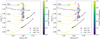Fig. 14

Same as Fig. 13, but for the observed TiO temperatures scaled by the J-band (left) and the i-band (right) relation.

5.3 Color-temperature relations

The different slopes of the empirically established relations by Britavskiy et al. (2019a,b), presented in the left panel of Fig. 10, cannot be explained by metallicity alone. A potential explanation could be the effect of a strong stellar wind on the spectral appearance of a RSG. Davies & Plez (2021) show that a significant stellar wind affects the flux in the K_S band, due to the increasing CO emission emerging from a circumstellar molecular shell. The effects of stellar winds are not incorporated in the MARCS models and are therefore not reflected in our theoretical T_eff(J − K_S) relation. CO emission starts around ~2.3 μm, which is at the edge of the K_S-band filter. Here, the efficiency of the filter has already significantly dropped, and the increasing flux due to molecular emission should not affect the K_S-band magnitude drastically. We therefore argue that the stellar wind cannot explain the change in the slope between the SMC and LMC relations. Another possible explanation may be the improper treatment of 3D processes (e.g., convection) in the 1D atmospheric models, either under-predicting or over-predicting the near-IR fluxes. However, for the example shown in Davies et al. (2013), fluxes in both J and K_S bands are relatively unaffected by the changes from 1D to 3D models (CO⁵BOLD; Freytag et al. 2002; Chiavassa et al. 2011). We therefore argue that the 3D-to-1D simplifications in the MARCS models cannot explain the observations either. More investigation is needed to explain the changing T_eff(J − K_S) relations with Z.

5.4 TiO bands as a potential $\dot{M}$ $\[\dot{M}\]$ diagnostic

Throughout this study (and others, e.g., Davies et al. 2013; Davies & Plez 2021), we argued that the TiO diagnostic is unsuitable for determining the effective temperature of a RSG. Here, we discuss the TiO bands as a possible diagnostic to probe mass loss. A strong stellar wind impacts the spectral appearance of a RSG spectrum in the optical (drastically so, in cases where $\dot{M}$ $\[\dot{M}\]$ > 10⁻⁵ M_⊙ yr⁻¹; Davies & Plez 2021). Therefore, if the other parameters that affect the TiO band strengths are known (i.e., T_eff and Z), they can be fixed in atmospheric modeling, and one can obtain the mass-loss rate. The first step is therefore to constrain T_eff and Z independently of the optical spectrum. Near-IR spectra, for example with X-shooter or K-band Multi-Object Spectrograph (KMOS), provide spectral lines to constrain both of these properties independently. One can then directly study the dependence of the mass-loss rate on Z, which is currently still debated. Furthermore, microturbulent velocities (υ_turb or ξ) can be obtained from the broadening of spectral lines by fitting, for example, MARCS model atmospheres (see, e.g., Davies et al. 2010, for an application on J-band spectral lines). Then, one can study the dependence of $\dot{M}$ $\[\dot{M}\]$ on turbulence. Kee et al. (2021) assumed turbulence to be the dominant mass-loss mechanism driving the RSG stellar wind. Quantifying the relation between turbulence and mass-loss rates using the TiO bands could therefore improve our understanding of the mass-loss mechanism for RSGs.

The next step would be to extend the MARCS models to allow $\dot{M}$ $\[\dot{M}\]$ to be fit. Pioneering work by Davies & Plez (2021) demonstrated the effect of adding RSG mass loss on top of the hydrostatic MARCS model atmospheres, reproducing most features arising from the circumstellar molecular sphere of RSGs (see González-Torà et al. 2023, 2024, for an application to CO transitions in the K band). A grid (for every combination of T_eff, Z, etc.) of such models incorporating stellar wind physics would potentially address several open questions about RSG mass loss. With improved models and tighter constraints on the stellar parameters of RSGs, we argue that the TiO bands can be a valuable mass-loss diagnostic, particularly due to their observational accessibility for RSGs out to a few megaparsecs. Many multi-object spectroscopic instruments exist, which could simultaneously observe the TiO bands for large populations of extragalactic RSGs (e.g., FORS2). Low-resolution spectra are sufficient to model the TiO bands, keeping exposure times to a minimum. In contrast, large distances render some existing mass-loss methods unfeasible, such as the CO transitions observed with ALMA (e.g., Decin et al. 2024). With the excellent spatial resolution and sensitivity of the James Webb Space Telescope, SED fitting of dust emission becomes possible for distant RSGs. However, such modeling still suffers from uncertain, yet high-impact assumptions, such as the gas-to-dust ratio, grain size distribution, and dust composition. We therefore conclude that the TiO bands have great potential as a direct $\dot{M}$ $\[\dot{M}\]$ diagnostic, especially at large distances.

6 Summary and conclusions

We have presented the physical parameters of the largest sample of spectroscopically studied RSGs (127) outside the Local Group (NGC 55, NGC 247, NGC 253, NGC 300, NGC 1313, NGC3109, NGC 7793, Sextans A, and M83, presented in Bonanos et al. 2024). Using SED fitting, we derived luminosities for 92 RSGs and find that ~50% have log(L/L_⊙) ≥ 5.0, of which six have extreme stellar radii (R ≳ 1400 R_⊙). We analyzed optical and mid-IR light curves to characterize RSG variability and found two very evolved RSGs (NGC300-59 and NGC55-40) that show significant variability in both their optical and mid-IR light curves. For all 127 RSG spectra, we present a refined spectral classification compared to Bonanos et al. (2024) and performed MARCS atmospheric modeling to derive their effective temperatures, extinction factors, and radial velocities.

Temperatures of RSGs are easily obtained through calibrated color-temperature relations, yet existing relations are either applicable to only one metallicity or were calibrated using only one temperature scale. We derived J − K_s color versus temperature relations from (i) the TiO bands, (ii) the J band, and (iii) synthetic photometry from the MARCS models for a range of metallicities, finding a Z-dependent color-temperature relation. A strong dependence of the empirical T_eff(J − K_S) relations on Z was established by Britavskiy et al. (2019a,b) but is not supported by the theoretical, synthetic relations derived in this work. This hints at an extra contribution to the J − K_S color that is missed by the physics incorporated in the MARCS models. Mass loss is one potential explanation, although it has been shown that the flux in both the J and K_S bands is relatively insensitive to the mass-loss rate (Davies & Plez 2021).

To bypass the limitations of the TiO diagnostic, we derived two scaling relations using temperatures from Davies et al. (2013, 2015) and Tabernero et al. (2018) and bridged the T_eff,TiO discrepancy. The extent of the discrepancy scales tightly with the mass-loss rate, in agreement with the increased TiO absorption for mass-losing RSGs shown by Davies & Plez (2021). We applied the scaling relation to our modeled T_eff,TiO and compared the results to evolutionary tracks. The i-band-scaled TiO temperatures are a good match to the core helium-burning stage of the POSYDON evolutionary tracks. A metallicity and mass-loss rate dependence of the scaling relations should be established in a future study.

We compared 33 dusty RSGs (m_3.6 − m_4.5 > 0.1 mag and M_3.6 ≤ −9.0 mag) to non-dusty RSGs and found that the dusty RSGs are on average (i) 60 K cooler, (ii) more extinct in the V band by ~0.6 mag, and (iii) more luminous by 0.21 dex, indicating that RSGs with circumstellar dust are generally more evolved. Their IR excess was therefore expected, as they are more likely to shed mass and form dust. Three dusty RSGs exceed the revised Humphreys-Davidson limit and have luminosities and stellar radii comparable to WOH G64. We also found three K-type RSGs with IR excess and speculate that they are candidate Levesque-Massey variables that may have transitioned from a cooler M-type RSG back to a hotter state in recent years. Alternatively, we speculate that they may have experienced a recent, anisotropic mass ejection outside the line of sight, which left the surface unobscured but enriched the circumstellar environment with dust.

Lastly, we propose that the TiO diagnostic has great potential to probe the mass-loss rates of RSGs. Following Davies & Plez (2021), who demonstrated the effects of mass loss on the RSG spectra, we tentatively argue that the existence of a complete grid of MARCS models that incorporates such effects could potentially benchmark a relation between mass loss and metallicity for RSGs. Obtaining microturbulent velocities from broadened spectral lines in high-resolution spectra (using, e.g., MARCS models) may provide empirical insights into the driving mechanism of RSG winds. We suggest that when Z and T_eff are known from near-IR spectroscopy (e.g., KMOS), the TiO bands could serve as a direct and easily accessible diagnostic to derive the mass-loss rates of distant RSGs.

Data availability

The full Tables 2 and 3 and spectral fits are available at the CDS via anonymous ftp to cdsarc.cds.unistra.fr (130.79.128.5) or via https://cdsarc.cds.unistra.fr/viz-bin/cat/J/A+A/689/A46

Acknowledgements

S.dW., A.Z.B., K.A., E.Z., E.C., G.M., and G.M.S. acknowledge funding support from the European Research Council (ERC) under the European Union’s Horizon 2020 research and innovation program (Grant agreement No. 772086. E.Z. also acknowledges support from the Hellenic Foundation for Research and Innovation (H.F.R.I.) under the “3rd Call for H.F.R.I. Research Projects to Support Post-Doctoral Researchers” (Project No: 7933). N.B. acknowledges support from the postdoctoral program (IPD-STEMA) of Liege University, and the Belgian federal government grant for Ukrainian postdoctoral researchers (contract UF/2022/10). K.D.’s work was supported by NASA through the NASA Hubble Fellowship grant #HST-HF2-51477.001 awarded by the Space Telescope Science Institute, which is operated by the Association of Universities for Research in Astronomy, Inc., for NASA, under contract NAS5-26555. Based on observations collected at the European Southern Observatory under ESO program 105.20HJ and 109.22W2. This research has made use of NASA’s Astrophysics Data System. This research has made use of the SVO Filter Profile Service (http://svo2.cab.inta-csic.es/theory/fps/) supported by the Spanish MINECO through grant AYA2017-84089. Spitzer: This work is based in part on observations made with the Spitzer Space Telescope, which is operated by the Jet Propulsion Laboratory, California Institute of Technology under a contract with NASA. Gaia: This work has made use of data from the European Space Agency (ESA) mission Gaia (https://www.cosmos.esa.int/gaia), processed by the Gaia Data Processing and Analysis Consortium (DPAC, https://www.cosmos.esa.int/web/gaia/dpac/consortium). Funding for the DPAC has been provided by national institutions, in particular, the institutions participating in the Gaia Multilateral Agreement. WISE: This publication makes use of data products from the Wide-field Infrared Survey Explorer, which is a joint project of the University of California, Los Angeles, and the Jet Propulsion Laboratory/California Institute of Technology, funded by the National Aeronautics and Space Administration. Pan-STARRS1: The Pan-STARRS1 Surveys (PS1) and the PS1 public science archive have been made possible through contributions by the Institute for Astronomy, the University of Hawaii, the Pan-STARRS Project Office, the Max-Planck Society and its participating institutes, the Max Planck Institute for Astronomy, Heidelberg and the Max Planck Institute for Extraterrestrial Physics, Garching, The Johns Hopkins University, Durham University, the University of Edinburgh, the Queen’s University Belfast, the Harvard-Smithsonian Center for Astrophysics, the Las Cumbres Observatory Global Telescope Network Incorporated, the National Central University of Taiwan, the Space Telescope Science Institute, the National Aeronautics and Space Administration under Grant No. NNX08AR22G issued through the Planetary Science Division of the NASA Science Mission Directorate, the National Science Foundation Grant No. AST-1238877, the University of Maryland, Eotvos Lorand University (ELTE), the Los Alamos National Laboratory, and the Gordon and Betty Moore Foundation. ATLAS: This work includes data from the Asteroid Terrestrial-impact Last Alert System (ATLAS) project. ATLAS is primarily funded to search for near-earth asteroids through NASA grants NN12AR55G, 80NSSC18K0284, and 80NSSC18K1575; byproducts of the NEO search include images and catalogs from the survey area. The ATLAS science products have been made possible through the contributions of the University of Hawaii Institute for Astronomy, the Queen’s University Belfast, the Space Telescope Science Institute, and the South African Astronomical Observatory.

Appendix A Supplementary figures

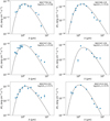Fig. A.1

Blackbody fits of the six extreme-luminosity RSGs presented in Sects. 5.1 and 5.2. The solid line is the best-fit black-body curve to the observed SED, which yields the luminosity. Blue diamonds show the photometric observations in different bands.

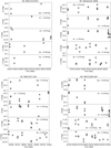Fig. A.2

Complete Pan-STARRS1 grizy light curves of four of the RSGs presented in Sec. 2.4 (NGC3109-167, SextansA-1906, NGC247-154, and NGC253-872).

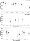Fig. A.3

Gaia light curves of NGC300-125, NGC247-3683, and NGC253-872, presented in Sect. 2.4.1.

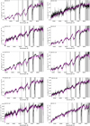Fig. A.4

Best-fit MARCS models to all RSG spectra.

References

Ahmad, A., Freytag, B., & Höfner, S. 2023, A&A, 669, A49 [NASA ADS] [CrossRef] [EDP Sciences] [Google Scholar]
Antoniadis, K., Bonanos, A. Z., de Wit, S., et al. 2024, A&A, 686, A88 [NASA ADS] [CrossRef] [EDP Sciences] [Google Scholar]
Beasor, E. R., & Smith, N. 2022, ApJ, 933, 41 [NASA ADS] [CrossRef] [Google Scholar]
Beasor, E. R., Davies, B., Smith, N., et al. 2020, MNRAS, 492, 5994 [Google Scholar]
Beasor, E. R., Davies, B., & Smith, N. 2021, ApJ, 922, 55 [NASA ADS] [CrossRef] [Google Scholar]
Bergemann, M., Lind, K., Collet, R., et al. 2012, MNRAS, 427, 27 [NASA ADS] [CrossRef] [Google Scholar]
Bergemann, M., Kudritzki, R.-P., Würl, M., et al. 2013, ApJ, 764, 115 [NASA ADS] [CrossRef] [Google Scholar]
Bergemann, M., Kudritzki, R.-P., Gazak, Z., et al. 2015, ApJ, 804, 113 [NASA ADS] [CrossRef] [Google Scholar]
Blagorodnova, N., Klencki, J., Pejcha, O., et al. 2021, A&A, 653, A134 [NASA ADS] [CrossRef] [EDP Sciences] [Google Scholar]
Boggs, P. T., & Rogers, J. E. 1990, Contemp. Math., 112, 183 [Google Scholar]
Bonanos, A. Z., Tramper, F., de Wit, S., et al. 2024, A&A, 686, A77 (Paper I) [NASA ADS] [CrossRef] [EDP Sciences] [Google Scholar]
Brands, S. A., de Koter, A., Bestenlehner, J. M., et al. 2023, A&A, 673, A132 [NASA ADS] [CrossRef] [EDP Sciences] [Google Scholar]
Bresolin, F., Kudritzki, R.-P., Urbaneja, M. A., et al. 2016, ApJ, 830, 64 [NASA ADS] [CrossRef] [Google Scholar]
Britavskiy, N., Lennon, D. J., Patrick, L. R., et al. 2019a, A&A, 624, A128 [NASA ADS] [CrossRef] [EDP Sciences] [Google Scholar]
Britavskiy, N. E., Bonanos, A. Z., Herrero, A., et al. 2019b, A&A, 631, A95 [NASA ADS] [CrossRef] [EDP Sciences] [Google Scholar]
Brott, I., de Mink, S. E., Cantiello, M., et al. 2011, A&A, 530, A115 [NASA ADS] [CrossRef] [EDP Sciences] [Google Scholar]
Bruch, R. J., Gal-Yam, A., Schulze, S., et al. 2021, ApJ, 912, 46 [NASA ADS] [CrossRef] [Google Scholar]
Buchner, J. 2021, J. Open Source Softw., 6, 3001 [CrossRef] [Google Scholar]
Carr, J. S., Sellgren, K., & Balachandran, S. C. 2000, ApJ, 530, 307 [NASA ADS] [CrossRef] [Google Scholar]
Chambers, K. C., Magnier, E. A., Metcalfe, N., et al. 2016, arXiv e-prints [arXiv:1612.05560] [Google Scholar]
Chiavassa, A., Freytag, B., Masseron, T., & Plez, B. 2011, A&A, 535, A22 [NASA ADS] [CrossRef] [EDP Sciences] [Google Scholar]
Chiavassa, A., Kravchenko, K., Montargès, M., et al. 2022, A&A, 658, A185 [NASA ADS] [CrossRef] [EDP Sciences] [Google Scholar]
Cutri, R. M., Skrutskie, M. F., van Dyk, S., et al. 2003, VizieR Online Data Catalog, II/246 [Google Scholar]
Davidge, T. J. 2021, AJ, 162, 152 [NASA ADS] [CrossRef] [Google Scholar]
Davies, B., & Beasor, E. R. 2020, MNRAS, 493, 468 [NASA ADS] [CrossRef] [Google Scholar]
Davies, B., & Plez, B. 2021, MNRAS, 508, 5757 [NASA ADS] [CrossRef] [Google Scholar]
Davies, B., Kudritzki, R.-P., & Figer, D. F. 2010, MNRAS, 407, 1203 [NASA ADS] [CrossRef] [Google Scholar]
Davies, B., Kudritzki, R.-P., Plez, B., et al. 2013, ApJ, 767, 3 [Google Scholar]
Davies, B., Kudritzki, R.-P., Gazak, Z., et al. 2015, ApJ, 806, 21 [NASA ADS] [CrossRef] [Google Scholar]
Davies, B., Crowther, P. A., & Beasor, E. R. 2018, MNRAS, 478, 3138 [NASA ADS] [CrossRef] [Google Scholar]
De, K., MacLeod, M., Karambelkar, V., et al. 2023, Nature, 617, 55 [NASA ADS] [CrossRef] [Google Scholar]
Decin, L. 2021, ARA&A, 59, 337 [NASA ADS] [CrossRef] [Google Scholar]
Decin, L., Richards, A. M. S., Marchant, P., & Sana, H. 2024, A&A, 681, A17 [NASA ADS] [CrossRef] [EDP Sciences] [Google Scholar]
de Jager, C. 1998, A&A Rev., 8, 145 [NASA ADS] [CrossRef] [Google Scholar]
de Jager, C., Nieuwenhuijzen, H., & van der Hucht, K. A. 1988, A&AS, 72, 259 [NASA ADS] [Google Scholar]
Della Bruna, L., Adamo, A., Lee, J. C., et al. 2021, A&A, 650, A103 [NASA ADS] [CrossRef] [EDP Sciences] [Google Scholar]
de Mink, S. E., Sana, H., Langer, N., et al. 2014, ApJ, 782, 7 [CrossRef] [Google Scholar]
de Wit, S., Bonanos, A. Z., Tramper, F., et al. 2023, A&A, 669, A86 [NASA ADS] [CrossRef] [EDP Sciences] [Google Scholar]
Ekström, S., Georgy, C., Eggenberger, P., et al. 2012, A&A, 537, A146 [Google Scholar]
Eldridge, J. J., Fraser, M., Smartt, S. J., et al. 2013, MNRAS, 436, 774 [NASA ADS] [CrossRef] [Google Scholar]
Eldridge, J. J., Xiao, L., Stanway, E. R., et al. 2018, PASA, 35, e049 [NASA ADS] [CrossRef] [Google Scholar]
Elias, J. H., Frogel, J. A., & Humphreys, R. M. 1985, ApJS, 57, 91 [NASA ADS] [CrossRef] [Google Scholar]
Evans, C. J., Bresolin, F., Urbaneja, M. A., et al. 2007, ApJ, 659, 1198 [Google Scholar]
Fazio, G. G., Hora, J. L., Allen, L. E., et al. 2004, ApJS, 154, 10 [Google Scholar]
Fitzpatrick, E. L. 1999, PASP, 111, 63 [Google Scholar]
Fragos, T., Andrews, J. J., Bavera, S. S., et al. 2023, ApJS, 264, 45 [NASA ADS] [CrossRef] [Google Scholar]
Freytag, B., Steffen, M., & Dorch, B. 2002, Astron. Nachr., 323, 213 [Google Scholar]
Gaia Collaboration (Vallenari, A., et al.) 2023, A&A, 674, A1 [NASA ADS] [CrossRef] [EDP Sciences] [Google Scholar]
Gazak, J. Z., Kudritzki, R., Evans, C., et al. 2015, ApJ, 805, 182 [NASA ADS] [CrossRef] [Google Scholar]
Georgy, C., Ekström, S., Eggenberger, P., et al. 2013, A&A, 558, A103 [NASA ADS] [CrossRef] [EDP Sciences] [Google Scholar]
Goldman, S. R., van Loon, J. T., Zijlstra, A. A., et al. 2017, MNRAS, 465, 403 [Google Scholar]
González-Torà, G., Davies, B., Kudritzki, R.-P., et al. 2021, MNRAS, 505, 4422 [CrossRef] [Google Scholar]
González-Torà, G., Wittkowski, M., Davies, B., et al. 2023, A&A, 669, A76 [NASA ADS] [CrossRef] [EDP Sciences] [Google Scholar]
González-Torà, G., Wittkowski, M., Davies, B., et al. 2024, A&A, 683, A19 [NASA ADS] [CrossRef] [EDP Sciences] [Google Scholar]
Gordon, M. S., & Humphreys, R. M. 2019, Galaxies, 7, 92 [NASA ADS] [CrossRef] [Google Scholar]
Groenewegen, M. A. T., & Sloan, G. C. 2018, A&A, 609, A114 [NASA ADS] [CrossRef] [EDP Sciences] [Google Scholar]
Gustafsson, B., Edvardsson, B., Eriksson, K., et al. 2008, A&A, 486, 951 [NASA ADS] [CrossRef] [EDP Sciences] [Google Scholar]
Hadfield, L. J., & Crowther, P. A. 2007, MNRAS, 381, 418 [CrossRef] [Google Scholar]
Hartoog, O. E., Sana, H., de Koter, A., & Kaper, L. 2012, MNRAS, 422, 367 [NASA ADS] [CrossRef] [Google Scholar]
Heger, A., Fryer, C. L., Woosley, S. E., et al. 2003, ApJ, 591, 288 [CrossRef] [Google Scholar]
Henyey, L., Vardya, M. S., & Bodenheimer, P. 1965, ApJ, 142, 841 [Google Scholar]
Hernandez, S., Larsen, S., Aloisi, A., et al. 2019, ApJ, 872, 116 [NASA ADS] [CrossRef] [Google Scholar]
Hlavacek-Larrondo, J., Carignan, C., Daigle, O., et al. 2011, MNRAS, 411, 71 [NASA ADS] [CrossRef] [Google Scholar]
Hosek, Matthew W., J., Kudritzki, R.-P., Bresolin, F., et al. 2014, ApJ, 785, 151 [NASA ADS] [CrossRef] [Google Scholar]
Humphreys, R. M., & Davidson, K. 1979, ApJ, 232, 409 [Google Scholar]
Humphreys, R. M., & Jones, T. J. 2022, AJ, 163, 103 [NASA ADS] [CrossRef] [Google Scholar]
Ivezic, Z., & Elitzur, M. 1997, MNRAS, 287, 799 [Google Scholar]
Jencson, J. E., Pearson, J., Beasor, E. R., et al. 2023, ApJ, 952, L30 [NASA ADS] [CrossRef] [Google Scholar]
Kee, N. D., Sundqvist, J. O., Decin, L., et al. 2021, A&A, 646, A180 [NASA ADS] [CrossRef] [EDP Sciences] [Google Scholar]
Kervella, P., Decin, L., Richards, A. M. S., et al. 2018, A&A, 609, A67 [NASA ADS] [CrossRef] [EDP Sciences] [Google Scholar]
Kilpatrick, C. D., Foley, R. J., Jacobson-Galán, W. V., et al. 2023, ApJ, 952, L23 [NASA ADS] [CrossRef] [Google Scholar]
Kiss, L. L., Szabó, G. M., & Bedding, T. R. 2006, MNRAS, 372, 1721 [Google Scholar]
Kniazev, A. Y., Grebel, E. K., Pustilnik, S. A., et al. 2005, AJ, 130, 1558 [NASA ADS] [CrossRef] [Google Scholar]
Koribalski, B. S., Staveley-Smith, L., Kilborn, V. A., et al. 2004, AJ, 128, 16 [Google Scholar]
Kravchenko, K., Chiavassa, A., Van Eck, S., et al. 2019, A&A, 632, A28 [NASA ADS] [CrossRef] [EDP Sciences] [Google Scholar]
Kravchenko, K., Jorissen, A., Van Eck, S., et al. 2021, A&A, 650, A17 [NASA ADS] [CrossRef] [EDP Sciences] [Google Scholar]
Kroupa, P. 2001, MNRAS, 322, 231 [NASA ADS] [CrossRef] [Google Scholar]
Kudritzki, R.-P., Urbaneja, M. A., Bresolin, F., et al. 2008, ApJ, 681, 269 [NASA ADS] [CrossRef] [Google Scholar]
Kurucz, R. L. 2005, Mem. Soc. Astron. Ital. Suppl., 8, 14 [Google Scholar]
Laplace, E., Götberg, Y., de Mink, S. E., et al. 2020, A&A, 637, A6 [NASA ADS] [CrossRef] [EDP Sciences] [Google Scholar]
Laplace, E., Justham, S., Renzo, M., et al. 2021, A&A, 656, A58 [NASA ADS] [CrossRef] [EDP Sciences] [Google Scholar]
Levesque, E. M. 2017, Astrophysics of Red Supergiants (Bristol, UK: IOP Publishing) [Google Scholar]
Levesque, E. M., & Massey, P. 2020, ApJ, 891, L37 [Google Scholar]
Levesque, E. M., Massey, P., Olsen, K. A. G., et al. 2005, ApJ, 628, 973 [Google Scholar]
Levesque, E. M., Massey, P., Olsen, K. A. G., et al. 2006, ApJ, 645, 1102 [NASA ADS] [CrossRef] [Google Scholar]
Levesque, E. M., Massey, P., Olsen, K. A. G., & Plez, B. 2007, ApJ, 667, 202 [NASA ADS] [CrossRef] [Google Scholar]
Levesque, E. M., Massey, P., Plez, B., & Olsen, K. A. G. 2009, AJ, 137, 4744 [NASA ADS] [CrossRef] [Google Scholar]
Ludwig, H. G., Behara, N. T., Steffen, M., & Bonifacio, P. 2009, A&A, 502, L1 [NASA ADS] [CrossRef] [EDP Sciences] [Google Scholar]
Ma, J.-Z., Chiavassa, A., de Mink, S. E., et al. 2024, ApJ, 962, L36 [NASA ADS] [CrossRef] [Google Scholar]
Madore, B. F., & Freedman, W. L. 2020, ApJ, 899, 66 [NASA ADS] [CrossRef] [Google Scholar]
Maíz Apellániz, J., Evans, C. J., Barbá, R. H., et al. 2014, A&A, 564, A63 [CrossRef] [EDP Sciences] [Google Scholar]
Maravelias, G., de Wit, S., Bonanos, A. Z., et al. 2023, Galaxies, 11, 79 [NASA ADS] [CrossRef] [Google Scholar]
Massey, P., Plez, B., Levesque, E. M., et al. 2005, ApJ, 634, 1286 [NASA ADS] [CrossRef] [Google Scholar]
Massey, P., Levesque, E. M., Olsen, K. A. G., et al. 2007, ApJ, 660, 301 [NASA ADS] [CrossRef] [Google Scholar]
Massey, P., Neugent, K. F., Ekström, S., et al. 2023, ApJ, 942, 69 [NASA ADS] [CrossRef] [Google Scholar]
McConnachie, A. W. 2012, AJ, 144, 4 [Google Scholar]
McMahon, R. 2012, in Science from the Next Generation Imaging and Spectroscopic Surveys, 37 [Google Scholar]
Meyer, M. J., Zwaan, M. A., Webster, R. L., et al. 2004, MNRAS, 350, 1195 [Google Scholar]
Meynet, G., & Maeder, A. 2000, A&A, 361, 101 [NASA ADS] [Google Scholar]
Meynet, G., Chomienne, V., Ekström, S., et al. 2015, A&A, 575, A60 [NASA ADS] [CrossRef] [EDP Sciences] [Google Scholar]
Montargès, M., Cannon, E., Lagadec, E., et al. 2021, Nature, 594, 365 [Google Scholar]
Munoz-Sanchez, G., de Wit, S., Bonanos, A. Z., et al. 2024, A&A, in press, https://doi.org/10.1051/0004-6361/202450737 [Google Scholar]
Neugent, K. F., Massey, P., Skiff, B., & Meynet, G. 2012, ApJ, 749, 177 [NASA ADS] [CrossRef] [Google Scholar]
Nieuwenhuijzen, H., & de Jager, C. 1990, A&A, 231, 134 [NASA ADS] [Google Scholar]
Onken, C. A., Wolf, C., Bessell, M. S., et al. 2019, PASA, 36, e033 [Google Scholar]
Patrick, L. R., Evans, C. J., Davies, B., et al. 2015, ApJ, 803, 14 [Google Scholar]
Patrick, L. R., Evans, C. J., Davies, B., et al. 2017, MNRAS, 468, 492 [NASA ADS] [CrossRef] [Google Scholar]
Patrick, L. R., Thilker, D., Lennon, D. J., et al. 2022, MNRAS, 513, 5847 [Google Scholar]
Paxton, B., Bildsten, L., Dotter, A., et al. 2011, ApJS, 192, 3 [Google Scholar]
Paxton, B., Cantiello, M., Arras, P., et al. 2013, ApJS, 208, 4 [Google Scholar]
Paxton, B., Marchant, P., Schwab, J., et al. 2015, ApJS, 220, 15 [Google Scholar]
Paxton, B., Schwab, J., Bauer, E. B., et al. 2018, ApJS, 234, 34 [NASA ADS] [CrossRef] [Google Scholar]
Possolo, A., Merkatas, C., & Bodnar, O. 2019, Metrologia, 56, 045009 [CrossRef] [Google Scholar]
Qing, G., Wang, W., Liu, J.-F., & Yoachim, P. 2015, ApJ, 799, 19 [NASA ADS] [CrossRef] [Google Scholar]
Rau, A., Kulkarni, S. R., Ofek, E. O., & Yan, L. 2007, ApJ, 659, 1536 [NASA ADS] [CrossRef] [Google Scholar]
Rieke, G. H., Young, E. T., Engelbracht, C. W., et al. 2004, ApJS, 154, 25 [Google Scholar]
Riello, M., De Angeli, F., Evans, D. W., et al. 2021, A&A, 649, A3 [NASA ADS] [CrossRef] [EDP Sciences] [Google Scholar]
Roman-Duval, J., Gordon, K. D., Meixner, M., et al. 2014, ApJ, 797, 86 [NASA ADS] [CrossRef] [Google Scholar]
Sana, H., de Mink, S. E., de Koter, A., et al. 2012, Science, 337, 444 [Google Scholar]
Schlafly, E. F., & Finkbeiner, D. P. 2011, ApJ, 737, 103 [Google Scholar]
Schlegel, D. J., Finkbeiner, D. P., & Davis, M. 1998, ApJ, 500, 525 [Google Scholar]
Schneider, F. R. N., Podsiadlowski, Ph., & Laplace, E. 2024, A&A, 686, A45 [NASA ADS] [CrossRef] [EDP Sciences] [Google Scholar]
Shiber, S., Chatzopoulos, E., Munson, B., & Frank, J. 2024, ApJ, 962, 168 [NASA ADS] [CrossRef] [Google Scholar]
Skilling, J. 2004, in American Institute of Physics Conference Series, 735, Bayesian Inference and Maximum Entropy Methods in Science and Engineering: 24th International Workshop on Bayesian Inference and Maximum Entropy Methods in Science and Engineering, eds. R. Fischer, R. Preuss, & U. V. Toussaint, 395 [Google Scholar]
Smartt, S. J., Eldridge, J. J., Crockett, R. M., & Maund, J. R. 2009, MNRAS, 395, 1409 [CrossRef] [Google Scholar]
Smith, N. 2014, ARA&A, 52, 487 [NASA ADS] [CrossRef] [Google Scholar]
Smith, N., Hinkle, K. H., & Ryde, N. 2009, AJ, 137, 3558 [NASA ADS] [CrossRef] [Google Scholar]
Soraisam, M. D., Szalai, T., Van Dyk, S. D., et al. 2023, ApJ, 957, 64 [NASA ADS] [CrossRef] [Google Scholar]
Spinoglio, L., Fernández-Ontiveros, J. A., Malkan, M. A., et al. 2022, ApJ, 926, 55 [NASA ADS] [CrossRef] [Google Scholar]
Sukhbold, T., Ertl, T., Woosley, S. E., et al. 2016, ApJ, 821, 38 [NASA ADS] [CrossRef] [Google Scholar]
Tabernero, H. M., Dorda, R., Negueruela, I., & González-Fernández, C. 2018, MNRAS, 476, 3106 [NASA ADS] [CrossRef] [Google Scholar]
Tammann, G. A., Reindl, B., & Sandage, A. 2011, A&A, 531, A134 [NASA ADS] [CrossRef] [EDP Sciences] [Google Scholar]
Tonry, J. L., Denneau, L., Heinze, A. N., et al. 2018, PASP, 130, 064505 [Google Scholar]
Tully, R. B., Courtois, H. M., & Sorce, J. G. 2016, AJ, 152, 50 [Google Scholar]
van Loon, J. T., Cioni, M. R. L., Zijlstra, A. A., & Loup, C. 2005, A&A, 438, 273 [NASA ADS] [CrossRef] [EDP Sciences] [Google Scholar]
Verhoelst, T., van der Zypen, N., Hony, S., et al. 2009, A&A, 498, 127 [NASA ADS] [CrossRef] [EDP Sciences] [Google Scholar]
Vink, J. S., & Sabhahit, G. N. 2023, A&A, 678, A3 [NASA ADS] [CrossRef] [EDP Sciences] [Google Scholar]
Vink, J. S., de Koter, A., & Lamers, H. J. G. L. M. 2001, A&A, 369, 574 [NASA ADS] [CrossRef] [EDP Sciences] [Google Scholar]
Wheeler, J. C., & Chatzopoulos, E. 2023, Astron. Geophys., 64, 3.11 [NASA ADS] [CrossRef] [Google Scholar]
Whitelock, P. A., Feast, M. W., van Loon, J. T., & Zijlstra, A. A. 2003, MNRAS, 342, 86 [NASA ADS] [CrossRef] [Google Scholar]
Williams, S. J., Bonanos, A. Z., Whitmore, B. C., et al. 2015, A&A, 578, A100 [NASA ADS] [CrossRef] [EDP Sciences] [Google Scholar]
Yang, M., & Jiang, B. W. 2011, ApJ, 727, 53 [NASA ADS] [CrossRef] [Google Scholar]
Yang, M., & Jiang, B. W. 2012, ApJ, 754, 35 [NASA ADS] [CrossRef] [Google Scholar]
Yang, M., Bonanos, A. Z., Jiang, B.-W., et al. 2018, A&A, 616, A175 [NASA ADS] [CrossRef] [EDP Sciences] [Google Scholar]
Yang, M., Bonanos, A. Z., Jiang, B.-W., et al. 2020, A&A, 639, A116 [NASA ADS] [CrossRef] [EDP Sciences] [Google Scholar]
Yang, M., Bonanos, A. Z., Jiang, B., et al. 2023, A&A, 676, A84 [NASA ADS] [CrossRef] [EDP Sciences] [Google Scholar]
Zapartas, E., de Mink, S. E., Van Dyk, S. D., et al. 2017, ApJ, 842, 125 [CrossRef] [Google Scholar]
Zapartas, E., de Mink, S. E., Justham, S., et al. 2019, A&A, 631, A5 [NASA ADS] [CrossRef] [EDP Sciences] [Google Scholar]
Zapartas, E., de Mink, S. E., Justham, S., et al. 2021, A&A, 645, A6 [NASA ADS] [CrossRef] [EDP Sciences] [Google Scholar]
Zgirski, B., Pietrzyński, G., Gieren, W., et al. 2021, ApJ, 916, 19 [NASA ADS] [CrossRef] [Google Scholar]

¹

The ASSESS website: http://assess.astro.noa.gr/

²

We used an online tool for each of the galaxies http://ned.ipac.caltech.edu/byname

All Tables

Table 1

Properties of the galaxies studied in this work.

In the text

Table 2

Photometric properties of our RSG sample (extract).

In the text

Table 3

Physical parameters of our RSG sample (extract).

In the text

Table 4

Average parameters of RSGs.

In the text

Table 5

Overview of the T_eff(J − K_S) relations.

In the text

Table 6

Parameters of dusty versus non-dusty RSGs.

In the text

All Figures

Fig. 1

Color magnitude diagrams of 129 studies RSGs. Left: [3.6]-[4.5] versus M_[36]. Gray background points are sources from the Spitzer point source catalog of NGC 300. The dashed lines indicate the region of prioritized sources described in Bonanos et al. (2024) and show some degree of IR excess. Right: zoomed-in view of 34 prioritized dusty targets (33 classified). Red to yellow colors indicate a shift in spectral type toward hotter RSGs. The gray circle indicates the unclassified RSG. Four dusty K-type RSGs are highlighted: NGC3109-167 (1), NGC55-244 (2), NGC55-202 (3), and M83-682 (4).

In the text

	Fig. 2 Distribution of spectral types of classified RSGs. Blue hatched bars show RSGs with IR excess (see the right panel of Fig. 1; 33 targets). The remaining RSGs (94) are shown with gray bars.
In the text

	Fig. 3 Gaia G-band (top), WISE1 (middle), and WISE2 (bottom) light curves for NGC300-59. A zoomed-in view around the peak of the Gaia measurements is shown on the right.
In the text

Fig. 4

WISE1 versus MAD_wise1 diagram for RSGs in NGC 55 and NGC 300. The color bar indicates the luminosity for each RSG, and the gray dots indicate cases where a luminosity was not obtained. Black stars indicate eight RSGs that were reported as variable in optical surveys. Open circles indicate dusty RSGs. The dashed black curve indicates the median MAD for non-dusty RSGs. Four RSGs with both optical variability and a high MAD value relative to their WISE1 magnitude are labeled.

In the text

	Fig. 5 Best-fit MARCS model to NGC55-174, an M0-M2 I star. The FORS2 spectrum is indicated in black, the medium-resolution MARCS model in magenta, and telluric contaminated regions in gray shades.
In the text

	Fig. 6 Uncertainties of the best-fit T_eff and E(B − V) of NGC55-174. The red cross indicates the best-fit solution. The blue shades indicate a decrease in the goodness-of-fit, with the 1σ-3σ limits shown with red contours.
In the text

	Fig. 7 Stellar radius versus luminosity for 92 RSGs. Circles indicate sources from the dusty sample, four of which (including three dusty ones) exceed the revised Humphreys-Davidson limit. Note that the most luminous point contains two overlapping extreme RSGs. WOH G64 is indicated for reference.
In the text

	Fig. 8 Normalized histogram of the T_eff distribution of our RSG sample for 0.7 Z_⊙ (NGC 253; top), 0.4 Z_⊙ (NGC 300, NGC 247, and NGC 7793; middle), and 0.3 Z_⊙ (NGC 55 and NGC 1313; bottom), excluding sources with flags 2–4.
In the text

Fig. 9

Comparison of our modeled T_eff with the average T_eff of literature studies on RSGs based on the line-free continuum method (red triangles), SED method (green inverted triangles), J-band spectral lines (yellow circles), TiO bands (magenta squares), and i-band spectral lines (cyan stars) in a range of metallicities. TiO results from this work are marked with a thick border; larger squares represent larger sample sizes. The solid black line represents the mean T_eff of a population of RSGs computed with the POSYDON population synthesis code (see Sec. 3.3). The gray shades indicate the standard deviation from the mean T_eff of the RSG population at each metallicity. NGC 300* includes NGC 300, NGC 247, and NGC 7793; NGC 55* includes NGC 55 and NGC 1313.

In the text

Fig. 10

Color-temperature relations at a range of metallicities. Left: new empirical T_eff(J − K_S) relations compared to relations from the literature. Black lines show our new empirical relations based on samples from Levesque et al. (2006, squares) and Davies et al. (2015, circles). Gray lines show the empirical relations from Britavskiy et al. (2019a, LMC i band) and Britavskiy et al. (2019b, SMC i band) and the theoretical relations from Neugent et al. (2012, MARCS) and Yang et al. (2020, atlas). Right: effect of metallicity on the new theoretical T_eff(J − K_S) relations. We demonstrate the relation for the LMC metallicity with a dash-dotted gray line and the fit from Neugent et al. (2012) with a solid blue line. The gray shaded area indicates the effect of metallicity between the most extreme values of our grid (0.1–1.8 Z_⊙).

In the text

Fig. 11

Scaling relations between T_eff,TiO and T_eff,J (left) and between T_eff,TiO and T_eff,i (right). The scattered data points and their uncertainties are taken from Davies et al. (2013, 2015). The thick black line indicates the best-fit scaling relation, the gray shaded band shows the combination of slopes and offsets acceptable within a 1σ uncertainty and the black dotted lines indicate the scatter on the best-fit relation. In red, we show a simple linear fit to the data when one excludes the effect of asymmetric uncertainties. We show a 1:1 relation for comparison. The color bar indicates the mass-loss rates obtained with DUSTY. The sizes of the markers increase proportionally to metallicity.

In the text

	Fig. 12 T_eff versus the mass-loss rate for both TiO temperatures (squares; Davies et al. 2013) and J-band temperatures (circles; Davies et al. 2015). Colors indicate the stellar luminosity, and symbol sizes scale with metallicity, as in Fig. 11. A simple linear fit (dashed line) is shown for guidance.
In the text

	Fig. 13 HRD with the observed RSGs in NGC 300 (gray circles), NGC 247 (magenta triangles), and NGC 7793 (cyan squares). Four POSYDON tracks from 8–25 M_⊙ computed for log(Z/Z_⊙) = −0.35 are shown. The color indicates the central helium abundance; the knots on the tracks indicate timesteps of 10 000 yr.
In the text

	Fig. 14 Same as Fig. 13, but for the observed TiO temperatures scaled by the J-band (left) and the i-band (right) relation.
In the text

	Fig. A.1 Blackbody fits of the six extreme-luminosity RSGs presented in Sects. 5.1 and 5.2. The solid line is the best-fit black-body curve to the observed SED, which yields the luminosity. Blue diamonds show the photometric observations in different bands.
In the text

	Fig. A.2 Complete Pan-STARRS1 grizy light curves of four of the RSGs presented in Sec. 2.4 (NGC3109-167, SextansA-1906, NGC247-154, and NGC253-872).
In the text

	Fig. A.3 Gaia light curves of NGC300-125, NGC247-3683, and NGC253-872, presented in Sect. 2.4.1.
In the text

	Fig. A.4 Best-fit MARCS models to all RSG spectra.
In the text

Current usage metrics show cumulative count of Article Views (full-text article views including HTML views, PDF and ePub downloads, according to the available data) and Abstracts Views on Vision4Press platform.

Data correspond to usage on the plateform after 2015. The current usage metrics is available 48-96 hours after online publication and is updated daily on week days.

Initial download of the metrics may take a while.

[1] Ahmad, A., Freytag, B., & Höfner, S. 2023, A&A, 669, A49 [NASA ADS] [CrossRef] [EDP Sciences] [Google Scholar]

[2] Antoniadis, K., Bonanos, A. Z., de Wit, S., et al. 2024, A&A, 686, A88 [NASA ADS] [CrossRef] [EDP Sciences] [Google Scholar]

[3] Beasor, E. R., & Smith, N. 2022, ApJ, 933, 41 [NASA ADS] [CrossRef] [Google Scholar]

[4] Beasor, E. R., Davies, B., Smith, N., et al. 2020, MNRAS, 492, 5994 [Google Scholar]

[5] Beasor, E. R., Davies, B., & Smith, N. 2021, ApJ, 922, 55 [NASA ADS] [CrossRef] [Google Scholar]

[6] Bergemann, M., Lind, K., Collet, R., et al. 2012, MNRAS, 427, 27 [NASA ADS] [CrossRef] [Google Scholar]

[7] Bergemann, M., Kudritzki, R.-P., Würl, M., et al. 2013, ApJ, 764, 115 [NASA ADS] [CrossRef] [Google Scholar]

[8] Bergemann, M., Kudritzki, R.-P., Gazak, Z., et al. 2015, ApJ, 804, 113 [NASA ADS] [CrossRef] [Google Scholar]

[9] Blagorodnova, N., Klencki, J., Pejcha, O., et al. 2021, A&A, 653, A134 [NASA ADS] [CrossRef] [EDP Sciences] [Google Scholar]

[10] Boggs, P. T., & Rogers, J. E. 1990, Contemp. Math., 112, 183 [Google Scholar]

[11] Bonanos, A. Z., Tramper, F., de Wit, S., et al. 2024, A&A, 686, A77 (Paper I) [NASA ADS] [CrossRef] [EDP Sciences] [Google Scholar]

[12] Brands, S. A., de Koter, A., Bestenlehner, J. M., et al. 2023, A&A, 673, A132 [NASA ADS] [CrossRef] [EDP Sciences] [Google Scholar]

[13] Bresolin, F., Kudritzki, R.-P., Urbaneja, M. A., et al. 2016, ApJ, 830, 64 [NASA ADS] [CrossRef] [Google Scholar]

[14] Britavskiy, N., Lennon, D. J., Patrick, L. R., et al. 2019a, A&A, 624, A128 [NASA ADS] [CrossRef] [EDP Sciences] [Google Scholar]

[15] Britavskiy, N. E., Bonanos, A. Z., Herrero, A., et al. 2019b, A&A, 631, A95 [NASA ADS] [CrossRef] [EDP Sciences] [Google Scholar]

[16] Brott, I., de Mink, S. E., Cantiello, M., et al. 2011, A&A, 530, A115 [NASA ADS] [CrossRef] [EDP Sciences] [Google Scholar]

[17] Bruch, R. J., Gal-Yam, A., Schulze, S., et al. 2021, ApJ, 912, 46 [NASA ADS] [CrossRef] [Google Scholar]

[18] Buchner, J. 2021, J. Open Source Softw., 6, 3001 [CrossRef] [Google Scholar]

[19] Carr, J. S., Sellgren, K., & Balachandran, S. C. 2000, ApJ, 530, 307 [NASA ADS] [CrossRef] [Google Scholar]

[20] Chambers, K. C., Magnier, E. A., Metcalfe, N., et al. 2016, arXiv e-prints [arXiv:1612.05560] [Google Scholar]

[21] Chiavassa, A., Freytag, B., Masseron, T., & Plez, B. 2011, A&A, 535, A22 [NASA ADS] [CrossRef] [EDP Sciences] [Google Scholar]

[22] Chiavassa, A., Kravchenko, K., Montargès, M., et al. 2022, A&A, 658, A185 [NASA ADS] [CrossRef] [EDP Sciences] [Google Scholar]

[23] Cutri, R. M., Skrutskie, M. F., van Dyk, S., et al. 2003, VizieR Online Data Catalog, II/246 [Google Scholar]

[24] Davidge, T. J. 2021, AJ, 162, 152 [NASA ADS] [CrossRef] [Google Scholar]

[25] Davies, B., & Beasor, E. R. 2020, MNRAS, 493, 468 [NASA ADS] [CrossRef] [Google Scholar]

[26] Davies, B., & Plez, B. 2021, MNRAS, 508, 5757 [NASA ADS] [CrossRef] [Google Scholar]

[27] Davies, B., Kudritzki, R.-P., & Figer, D. F. 2010, MNRAS, 407, 1203 [NASA ADS] [CrossRef] [Google Scholar]

[28] Davies, B., Kudritzki, R.-P., Plez, B., et al. 2013, ApJ, 767, 3 [Google Scholar]

[29] Davies, B., Kudritzki, R.-P., Gazak, Z., et al. 2015, ApJ, 806, 21 [NASA ADS] [CrossRef] [Google Scholar]

[30] Davies, B., Crowther, P. A., & Beasor, E. R. 2018, MNRAS, 478, 3138 [NASA ADS] [CrossRef] [Google Scholar]

[31] De, K., MacLeod, M., Karambelkar, V., et al. 2023, Nature, 617, 55 [NASA ADS] [CrossRef] [Google Scholar]

[32] Decin, L. 2021, ARA&A, 59, 337 [NASA ADS] [CrossRef] [Google Scholar]

[33] Decin, L., Richards, A. M. S., Marchant, P., & Sana, H. 2024, A&A, 681, A17 [NASA ADS] [CrossRef] [EDP Sciences] [Google Scholar]

[34] de Jager, C. 1998, A&A Rev., 8, 145 [NASA ADS] [CrossRef] [Google Scholar]

[35] de Jager, C., Nieuwenhuijzen, H., & van der Hucht, K. A. 1988, A&AS, 72, 259 [NASA ADS] [Google Scholar]

[36] Della Bruna, L., Adamo, A., Lee, J. C., et al. 2021, A&A, 650, A103 [NASA ADS] [CrossRef] [EDP Sciences] [Google Scholar]

[37] de Mink, S. E., Sana, H., Langer, N., et al. 2014, ApJ, 782, 7 [CrossRef] [Google Scholar]

[38] de Wit, S., Bonanos, A. Z., Tramper, F., et al. 2023, A&A, 669, A86 [NASA ADS] [CrossRef] [EDP Sciences] [Google Scholar]

[39] Ekström, S., Georgy, C., Eggenberger, P., et al. 2012, A&A, 537, A146 [Google Scholar]

[40] Eldridge, J. J., Fraser, M., Smartt, S. J., et al. 2013, MNRAS, 436, 774 [NASA ADS] [CrossRef] [Google Scholar]

[41] Eldridge, J. J., Xiao, L., Stanway, E. R., et al. 2018, PASA, 35, e049 [NASA ADS] [CrossRef] [Google Scholar]

[42] Elias, J. H., Frogel, J. A., & Humphreys, R. M. 1985, ApJS, 57, 91 [NASA ADS] [CrossRef] [Google Scholar]

[43] Evans, C. J., Bresolin, F., Urbaneja, M. A., et al. 2007, ApJ, 659, 1198 [Google Scholar]

[44] Fazio, G. G., Hora, J. L., Allen, L. E., et al. 2004, ApJS, 154, 10 [Google Scholar]

[45] Fitzpatrick, E. L. 1999, PASP, 111, 63 [Google Scholar]

[46] Fragos, T., Andrews, J. J., Bavera, S. S., et al. 2023, ApJS, 264, 45 [NASA ADS] [CrossRef] [Google Scholar]

[47] Freytag, B., Steffen, M., & Dorch, B. 2002, Astron. Nachr., 323, 213 [Google Scholar]

[48] Gaia Collaboration (Vallenari, A., et al.) 2023, A&A, 674, A1 [NASA ADS] [CrossRef] [EDP Sciences] [Google Scholar]

[49] Gazak, J. Z., Kudritzki, R., Evans, C., et al. 2015, ApJ, 805, 182 [NASA ADS] [CrossRef] [Google Scholar]

[50] Georgy, C., Ekström, S., Eggenberger, P., et al. 2013, A&A, 558, A103 [NASA ADS] [CrossRef] [EDP Sciences] [Google Scholar]

[51] Goldman, S. R., van Loon, J. T., Zijlstra, A. A., et al. 2017, MNRAS, 465, 403 [Google Scholar]

[52] González-Torà, G., Davies, B., Kudritzki, R.-P., et al. 2021, MNRAS, 505, 4422 [CrossRef] [Google Scholar]

[53] González-Torà, G., Wittkowski, M., Davies, B., et al. 2023, A&A, 669, A76 [NASA ADS] [CrossRef] [EDP Sciences] [Google Scholar]

[54] González-Torà, G., Wittkowski, M., Davies, B., et al. 2024, A&A, 683, A19 [NASA ADS] [CrossRef] [EDP Sciences] [Google Scholar]

[55] Gordon, M. S., & Humphreys, R. M. 2019, Galaxies, 7, 92 [NASA ADS] [CrossRef] [Google Scholar]

[56] Groenewegen, M. A. T., & Sloan, G. C. 2018, A&A, 609, A114 [NASA ADS] [CrossRef] [EDP Sciences] [Google Scholar]

[57] Gustafsson, B., Edvardsson, B., Eriksson, K., et al. 2008, A&A, 486, 951 [NASA ADS] [CrossRef] [EDP Sciences] [Google Scholar]

[58] Hadfield, L. J., & Crowther, P. A. 2007, MNRAS, 381, 418 [CrossRef] [Google Scholar]

[59] Hartoog, O. E., Sana, H., de Koter, A., & Kaper, L. 2012, MNRAS, 422, 367 [NASA ADS] [CrossRef] [Google Scholar]

[60] Heger, A., Fryer, C. L., Woosley, S. E., et al. 2003, ApJ, 591, 288 [CrossRef] [Google Scholar]

[61] Henyey, L., Vardya, M. S., & Bodenheimer, P. 1965, ApJ, 142, 841 [Google Scholar]

[62] Hernandez, S., Larsen, S., Aloisi, A., et al. 2019, ApJ, 872, 116 [NASA ADS] [CrossRef] [Google Scholar]

[63] Hlavacek-Larrondo, J., Carignan, C., Daigle, O., et al. 2011, MNRAS, 411, 71 [NASA ADS] [CrossRef] [Google Scholar]

[64] Hosek, Matthew W., J., Kudritzki, R.-P., Bresolin, F., et al. 2014, ApJ, 785, 151 [NASA ADS] [CrossRef] [Google Scholar]

[65] Humphreys, R. M., & Davidson, K. 1979, ApJ, 232, 409 [Google Scholar]

[66] Humphreys, R. M., & Jones, T. J. 2022, AJ, 163, 103 [NASA ADS] [CrossRef] [Google Scholar]

[67] Ivezic, Z., & Elitzur, M. 1997, MNRAS, 287, 799 [Google Scholar]

[68] Jencson, J. E., Pearson, J., Beasor, E. R., et al. 2023, ApJ, 952, L30 [NASA ADS] [CrossRef] [Google Scholar]

[69] Kee, N. D., Sundqvist, J. O., Decin, L., et al. 2021, A&A, 646, A180 [NASA ADS] [CrossRef] [EDP Sciences] [Google Scholar]

[70] Kervella, P., Decin, L., Richards, A. M. S., et al. 2018, A&A, 609, A67 [NASA ADS] [CrossRef] [EDP Sciences] [Google Scholar]

[71] Kilpatrick, C. D., Foley, R. J., Jacobson-Galán, W. V., et al. 2023, ApJ, 952, L23 [NASA ADS] [CrossRef] [Google Scholar]

[72] Kiss, L. L., Szabó, G. M., & Bedding, T. R. 2006, MNRAS, 372, 1721 [Google Scholar]

[73] Kniazev, A. Y., Grebel, E. K., Pustilnik, S. A., et al. 2005, AJ, 130, 1558 [NASA ADS] [CrossRef] [Google Scholar]

[74] Koribalski, B. S., Staveley-Smith, L., Kilborn, V. A., et al. 2004, AJ, 128, 16 [Google Scholar]

[75] Kravchenko, K., Chiavassa, A., Van Eck, S., et al. 2019, A&A, 632, A28 [NASA ADS] [CrossRef] [EDP Sciences] [Google Scholar]

[76] Kravchenko, K., Jorissen, A., Van Eck, S., et al. 2021, A&A, 650, A17 [NASA ADS] [CrossRef] [EDP Sciences] [Google Scholar]

[77] Kroupa, P. 2001, MNRAS, 322, 231 [NASA ADS] [CrossRef] [Google Scholar]

[78] Kudritzki, R.-P., Urbaneja, M. A., Bresolin, F., et al. 2008, ApJ, 681, 269 [NASA ADS] [CrossRef] [Google Scholar]

[79] Kurucz, R. L. 2005, Mem. Soc. Astron. Ital. Suppl., 8, 14 [Google Scholar]

[80] Laplace, E., Götberg, Y., de Mink, S. E., et al. 2020, A&A, 637, A6 [NASA ADS] [CrossRef] [EDP Sciences] [Google Scholar]

[81] Laplace, E., Justham, S., Renzo, M., et al. 2021, A&A, 656, A58 [NASA ADS] [CrossRef] [EDP Sciences] [Google Scholar]

[82] Levesque, E. M. 2017, Astrophysics of Red Supergiants (Bristol, UK: IOP Publishing) [Google Scholar]

[83] Levesque, E. M., & Massey, P. 2020, ApJ, 891, L37 [Google Scholar]

[84] Levesque, E. M., Massey, P., Olsen, K. A. G., et al. 2005, ApJ, 628, 973 [Google Scholar]

[85] Levesque, E. M., Massey, P., Olsen, K. A. G., et al. 2006, ApJ, 645, 1102 [NASA ADS] [CrossRef] [Google Scholar]

[86] Levesque, E. M., Massey, P., Olsen, K. A. G., & Plez, B. 2007, ApJ, 667, 202 [NASA ADS] [CrossRef] [Google Scholar]

[87] Levesque, E. M., Massey, P., Plez, B., & Olsen, K. A. G. 2009, AJ, 137, 4744 [NASA ADS] [CrossRef] [Google Scholar]

[88] Ludwig, H. G., Behara, N. T., Steffen, M., & Bonifacio, P. 2009, A&A, 502, L1 [NASA ADS] [CrossRef] [EDP Sciences] [Google Scholar]

[89] Ma, J.-Z., Chiavassa, A., de Mink, S. E., et al. 2024, ApJ, 962, L36 [NASA ADS] [CrossRef] [Google Scholar]

[90] Madore, B. F., & Freedman, W. L. 2020, ApJ, 899, 66 [NASA ADS] [CrossRef] [Google Scholar]

[91] Maíz Apellániz, J., Evans, C. J., Barbá, R. H., et al. 2014, A&A, 564, A63 [CrossRef] [EDP Sciences] [Google Scholar]

[92] Maravelias, G., de Wit, S., Bonanos, A. Z., et al. 2023, Galaxies, 11, 79 [NASA ADS] [CrossRef] [Google Scholar]

[93] Massey, P., Plez, B., Levesque, E. M., et al. 2005, ApJ, 634, 1286 [NASA ADS] [CrossRef] [Google Scholar]

[94] Massey, P., Levesque, E. M., Olsen, K. A. G., et al. 2007, ApJ, 660, 301 [NASA ADS] [CrossRef] [Google Scholar]

[95] Massey, P., Neugent, K. F., Ekström, S., et al. 2023, ApJ, 942, 69 [NASA ADS] [CrossRef] [Google Scholar]

[96] McConnachie, A. W. 2012, AJ, 144, 4 [Google Scholar]

[97] McMahon, R. 2012, in Science from the Next Generation Imaging and Spectroscopic Surveys, 37 [Google Scholar]

[98] Meyer, M. J., Zwaan, M. A., Webster, R. L., et al. 2004, MNRAS, 350, 1195 [Google Scholar]

[99] Meynet, G., & Maeder, A. 2000, A&A, 361, 101 [NASA ADS] [Google Scholar]

[100] Meynet, G., Chomienne, V., Ekström, S., et al. 2015, A&A, 575, A60 [NASA ADS] [CrossRef] [EDP Sciences] [Google Scholar]

[101] Montargès, M., Cannon, E., Lagadec, E., et al. 2021, Nature, 594, 365 [Google Scholar]

[102] Munoz-Sanchez, G., de Wit, S., Bonanos, A. Z., et al. 2024, A&A, in press, https://doi.org/10.1051/0004-6361/202450737 [Google Scholar]

[103] Neugent, K. F., Massey, P., Skiff, B., & Meynet, G. 2012, ApJ, 749, 177 [NASA ADS] [CrossRef] [Google Scholar]

[104] Nieuwenhuijzen, H., & de Jager, C. 1990, A&A, 231, 134 [NASA ADS] [Google Scholar]

[105] Onken, C. A., Wolf, C., Bessell, M. S., et al. 2019, PASA, 36, e033 [Google Scholar]

[106] Patrick, L. R., Evans, C. J., Davies, B., et al. 2015, ApJ, 803, 14 [Google Scholar]

[107] Patrick, L. R., Evans, C. J., Davies, B., et al. 2017, MNRAS, 468, 492 [NASA ADS] [CrossRef] [Google Scholar]

[108] Patrick, L. R., Thilker, D., Lennon, D. J., et al. 2022, MNRAS, 513, 5847 [Google Scholar]

[109] Paxton, B., Bildsten, L., Dotter, A., et al. 2011, ApJS, 192, 3 [Google Scholar]

[110] Paxton, B., Cantiello, M., Arras, P., et al. 2013, ApJS, 208, 4 [Google Scholar]

[111] Paxton, B., Marchant, P., Schwab, J., et al. 2015, ApJS, 220, 15 [Google Scholar]

[112] Paxton, B., Schwab, J., Bauer, E. B., et al. 2018, ApJS, 234, 34 [NASA ADS] [CrossRef] [Google Scholar]

[113] Possolo, A., Merkatas, C., & Bodnar, O. 2019, Metrologia, 56, 045009 [CrossRef] [Google Scholar]

[114] Qing, G., Wang, W., Liu, J.-F., & Yoachim, P. 2015, ApJ, 799, 19 [NASA ADS] [CrossRef] [Google Scholar]

[115] Rau, A., Kulkarni, S. R., Ofek, E. O., & Yan, L. 2007, ApJ, 659, 1536 [NASA ADS] [CrossRef] [Google Scholar]

[116] Rieke, G. H., Young, E. T., Engelbracht, C. W., et al. 2004, ApJS, 154, 25 [Google Scholar]

[117] Riello, M., De Angeli, F., Evans, D. W., et al. 2021, A&A, 649, A3 [NASA ADS] [CrossRef] [EDP Sciences] [Google Scholar]

[118] Roman-Duval, J., Gordon, K. D., Meixner, M., et al. 2014, ApJ, 797, 86 [NASA ADS] [CrossRef] [Google Scholar]

[119] Sana, H., de Mink, S. E., de Koter, A., et al. 2012, Science, 337, 444 [Google Scholar]

[120] Schlafly, E. F., & Finkbeiner, D. P. 2011, ApJ, 737, 103 [Google Scholar]

[121] Schlegel, D. J., Finkbeiner, D. P., & Davis, M. 1998, ApJ, 500, 525 [Google Scholar]

[122] Schneider, F. R. N., Podsiadlowski, Ph., & Laplace, E. 2024, A&A, 686, A45 [NASA ADS] [CrossRef] [EDP Sciences] [Google Scholar]

[123] Shiber, S., Chatzopoulos, E., Munson, B., & Frank, J. 2024, ApJ, 962, 168 [NASA ADS] [CrossRef] [Google Scholar]

[124] Skilling, J. 2004, in American Institute of Physics Conference Series, 735, Bayesian Inference and Maximum Entropy Methods in Science and Engineering: 24th International Workshop on Bayesian Inference and Maximum Entropy Methods in Science and Engineering, eds. R. Fischer, R. Preuss, & U. V. Toussaint, 395 [Google Scholar]

[125] Smartt, S. J., Eldridge, J. J., Crockett, R. M., & Maund, J. R. 2009, MNRAS, 395, 1409 [CrossRef] [Google Scholar]

[126] Smith, N. 2014, ARA&A, 52, 487 [NASA ADS] [CrossRef] [Google Scholar]

[127] Smith, N., Hinkle, K. H., & Ryde, N. 2009, AJ, 137, 3558 [NASA ADS] [CrossRef] [Google Scholar]

[128] Soraisam, M. D., Szalai, T., Van Dyk, S. D., et al. 2023, ApJ, 957, 64 [NASA ADS] [CrossRef] [Google Scholar]

[129] Spinoglio, L., Fernández-Ontiveros, J. A., Malkan, M. A., et al. 2022, ApJ, 926, 55 [NASA ADS] [CrossRef] [Google Scholar]

[130] Sukhbold, T., Ertl, T., Woosley, S. E., et al. 2016, ApJ, 821, 38 [NASA ADS] [CrossRef] [Google Scholar]

[131] Tabernero, H. M., Dorda, R., Negueruela, I., & González-Fernández, C. 2018, MNRAS, 476, 3106 [NASA ADS] [CrossRef] [Google Scholar]

[132] Tammann, G. A., Reindl, B., & Sandage, A. 2011, A&A, 531, A134 [NASA ADS] [CrossRef] [EDP Sciences] [Google Scholar]

[133] Tonry, J. L., Denneau, L., Heinze, A. N., et al. 2018, PASP, 130, 064505 [Google Scholar]

[134] Tully, R. B., Courtois, H. M., & Sorce, J. G. 2016, AJ, 152, 50 [Google Scholar]

[135] van Loon, J. T., Cioni, M. R. L., Zijlstra, A. A., & Loup, C. 2005, A&A, 438, 273 [NASA ADS] [CrossRef] [EDP Sciences] [Google Scholar]

[136] Verhoelst, T., van der Zypen, N., Hony, S., et al. 2009, A&A, 498, 127 [NASA ADS] [CrossRef] [EDP Sciences] [Google Scholar]

[137] Vink, J. S., & Sabhahit, G. N. 2023, A&A, 678, A3 [NASA ADS] [CrossRef] [EDP Sciences] [Google Scholar]

[138] Vink, J. S., de Koter, A., & Lamers, H. J. G. L. M. 2001, A&A, 369, 574 [NASA ADS] [CrossRef] [EDP Sciences] [Google Scholar]

[139] Wheeler, J. C., & Chatzopoulos, E. 2023, Astron. Geophys., 64, 3.11 [NASA ADS] [CrossRef] [Google Scholar]

[140] Whitelock, P. A., Feast, M. W., van Loon, J. T., & Zijlstra, A. A. 2003, MNRAS, 342, 86 [NASA ADS] [CrossRef] [Google Scholar]

[141] Williams, S. J., Bonanos, A. Z., Whitmore, B. C., et al. 2015, A&A, 578, A100 [NASA ADS] [CrossRef] [EDP Sciences] [Google Scholar]

[142] Yang, M., & Jiang, B. W. 2011, ApJ, 727, 53 [NASA ADS] [CrossRef] [Google Scholar]

[143] Yang, M., & Jiang, B. W. 2012, ApJ, 754, 35 [NASA ADS] [CrossRef] [Google Scholar]

[144] Yang, M., Bonanos, A. Z., Jiang, B.-W., et al. 2018, A&A, 616, A175 [NASA ADS] [CrossRef] [EDP Sciences] [Google Scholar]

[145] Yang, M., Bonanos, A. Z., Jiang, B.-W., et al. 2020, A&A, 639, A116 [NASA ADS] [CrossRef] [EDP Sciences] [Google Scholar]

[146] Yang, M., Bonanos, A. Z., Jiang, B., et al. 2023, A&A, 676, A84 [NASA ADS] [CrossRef] [EDP Sciences] [Google Scholar]

[147] Zapartas, E., de Mink, S. E., Van Dyk, S. D., et al. 2017, ApJ, 842, 125 [CrossRef] [Google Scholar]