| Issue |
A&A
Volume 669, January 2023
|
|
|---|---|---|
| Article Number | A86 | |
| Number of page(s) | 16 | |
| Section | Stellar atmospheres | |
| DOI | https://doi.org/10.1051/0004-6361/202243394 | |
| Published online | 17 January 2023 | |
Properties of luminous red supergiant stars in the Magellanic Clouds
1
IAASARS, National Observatory of Athens,
15326
Penteli, Greece
e-mail: This email address is being protected from spambots. You need JavaScript enabled to view it.
2
National and Kapodistrian University of Athens, Department of Physics, Panepistimiopolis,
Zografos
15784, Greece
3
Institute of Astronomy, KU Leuven,
Celestijnlaan 200D,
3001
Leuven, Belgium
4
Key Laboratory of Space Astronomy and Technology, National Astronomical Observatories, Chinese Academy of Sciences,
Beijing
100101, PR China
5
Institute of Astrophysics FORTH,
71110
Heraklion, Greece
6
Carnegie Observatories, Las Campanas Observatory, Colina El Pino,
Casilla 601,
La Serena, Chile
7
University of Liège,
19C Allée du Six-Août (B5C),
4000
Sart Tilman, Liège, Belgium
8
Department of Astronomy, University of Geneva,
Chemin Pegasi 51,
1290
Versoix, Switzerland
Received:
22
February
2022
Accepted:
20
September
2022
Abstract
Context. There is evidence that some red supergiants (RSGs) experience short-lived phases of extreme mass loss, producing copious amounts of dust. These episodic outburst phases help strip the hydrogen envelope from evolved massive stars, drastically affecting their evolution. However, to date, the observational data of episodic mass loss is limited.
Aims. This paper aims to derive surface properties of a spectroscopic sample of 14 dusty sources in the Magellanic Clouds using the Baade telescope. These properties can be used for future spectral energy distribution fitting studies to measure the mass-loss rates from present circumstellar dust expelled from the star through outbursts.
Methods. We applied MARCS models to obtain the effective temperature (Teff) and extinction (AV) from the optical TiO bands. We used a χ2 routine to determine the model that best fits the obtained spectra. We computed the Teff using empirical photometric relations and compared this to our modelled Teff.
Results. We have identified a new yellow supergiant and spectroscopically confirmed eight new RSGs and one bright giant in the Magellanic Clouds. Additionally, we observed a supergiant B[e] star and find that the spectral type has changed compared to previous classifications, confirming that the spectral type is variable over decades. For the RSGs, we obtained the surface and global properties, as well as the extinction (AV).
Conclusions. Our method has picked up eight new, luminous RSGs. Despite selecting dusty RSGs, we find values for AV that are not as high as expected given the circumstellar extinction of these evolved stars. The most remarkable object from the sample, LMC3, is an extremely massive and luminous evolved massive star and may be grouped amongst the largest and most luminous RSGs known in the Large Magellanic Cloud (log(L*/L⊙) ~ 5.5 and R = 1400 R⊙).
Key words: stars: massive / supergiants / stars: fundamental parameters / stars: atmospheres / stars: late-type / Magellanic Clouds
© The Authors 2023
 Open Access article, published by EDP Sciences, under the terms of the Creative Commons Attribution License (https://creativecommons.org/licenses/by/4.0), which permits unrestricted use, distribution, and reproduction in any medium, provided the original work is properly cited.
This article is published in open access under the Subscribe-to-Open model. This email address is being protected from spambots. You need JavaScript enabled to view it. to support open access publication.
1 Introduction
The red supergiant (RSG) phase is the last evolutionary phase for the majority of massive stars (Levesque 2017). Red supergiants are subject to intense mass loss through stellar winds and outbursts (i.e. short-lived phases of extreme mass loss; see Smith 2014, for a review). These outbursts remain poorly constrained despite increasing evidence supporting their existence (Prieto et al. 2008; Mauerhan et al. 2013; Bruch et al. 2021; Humphreys & Jones 2022). The ability to potentially strip massive stars of their hydrogen envelope may drastically affect the course of their evolution in the latest stages before supernova collapse. At present, stellar evolutionary models for single stars (e.g. Eggenberger et al. 2008, 2021; Brott et al. 2011; Ekström et al. 2012; Köhler et al. 2015) or for binary stars (e.g. BPASS; Stanway & Eldridge 2018) adopt a continuous mass-loss rate, strongly influencing the type of supernova event. One approach for understanding episodic mass loss in evolved massive stars is to study the stellar properties of these stars empirically and test whether the derived properties can be recovered by existing evolutionary predictions. Several recent works have studied the mass-loss properties (e.g. Beasor et al. 2020, 2021) and stellar properties (e.g. Massey et al. 2021; González-Torà et al. 2021) of stars in the RSG phase. Interestingly, Beasor et al. (2020, 2021) find the mass-loss rates in the RSG phase to be lower than those of classical recipes (i.e. de Jager et al. 1988; van Loon et al. 2005), predicting that most single stars fail to remove their hydrogen-rich envelope and therefore should explode as a type-IIP supernova. This is inconsistent with the lack of observed high mass type-IIP progenitor stars, known as the ‘red supergiant problem’ (Smartt et al. 2009; Smartt 2015; Davies & Beasor 2020). The solution to this contradiction may either reside in the poorly understood short-lived phases (~104 yr; Beasor et al. 2020) of extreme mass loss, in addition to outbursts in the last years before the supernova explosion that results in a type-IIn supernova (Smith et al. 2009; Smith 2014), or in the stripping of the envelope due to binary interactions (Podsiadlowski et al. 1992; Eldridge et al. 2013; Zapartas et al. 2017).
The mass-loss rates of RSGs can be measured using spectral energy distribution (SED) fitting techniques (e.g. DUSTY; Ivezic & Elitzur 1997). Red supergiants can reveal an excess emission due to circumstellar dust as a result of slow and thick stellar winds in the RSG phase. When an object is surrounded by circumstellar dust, one can derive the contribution from the central component and the dust component by fitting the shape of the full SED (Goldman et al. 2017, Yang et al., in prep.). Reliable mid-IR photometry for modelling the dust emission bumps (i.e. 10 µm and 18 µm silicate emission and 11.3 µm polycyclic aromatic hydrocarbon emission; Jones et al. 2017) is vital, but such data are scarce due to instrument limitations, especially for more distant galaxies. Constraining the properties of the central source through spectroscopy eliminates potential degeneracies and uncertainties in the SED fitting procedure, greatly reducing the number of viable models for fitting the SED. To assess the mass loss, we therefore first need to derive accurate stellar parameters, such as the effective temperature of the central source. We approach this by targeting RSGs in the Large Magellanic Cloud (LMC) and Small Magellanic Cloud (SMC), using selection criteria from the near-IR and mid-IR (e.g. Bonanos et al. 2009, 2010; Britavskiy et al. 2014), to look for potential dust-obscured RSGs. In recent decades, various methods have been applied to derive the properties of RSGs. Using the MARCS model atmospheres (Gustafsson et al. 2008), Davies et al. (2013) and González-Torà et al. (2021) have fitted the shape of the SED, while Davies et al. (2015) and Tabernero et al. (2018) have used these models to fit spectral lines in the J and I band, respectively. In our work, however, as we had access to optical spectra, we used a similar approach to Levesque et al. (2005, 2006), measuring the effective temperature from the depths of the optical TiO bands.
In Sect. 2, we discuss the selection of targets and describe the spectroscopic observations, data reduction, and spectral classification of the spectra. We present the results of spectral modelling in Sect. 3 and compare them to empirical photometric relations and stellar evolutionary models. In Sect. 4, we compare the methodology and results to other, similar studies and present the conclusions in Sect. 5.
2 Target selection and observations
2.1 Target selection
We based our target selection on foreground-cleaned, multi-wavelength photometric catalogues for the SMC (Yang et al. 2019) and LMC (Yang et al. 2021). These extensive catalogues comprise many photometric datasets, including Gaia (Gaia Collaboration 2016, 2018), Spitzer (Werner et al. 2004), and 2MASS (Cutri et al. 2003; Skrutskie et al. 2006) photometry for numerous evolved massive stars in the Magellanic Clouds. To properly select dusty supergiant candidates, we used a set of criteria to distinguish them from the asymptotic giant branch (AGB) population. Following a similar approach to Britavskiy et al. (2014), we used the following set of criteria: (i) M[3,6] < −8 mag (see Britavskiy et al. 2014); (ii) J − [3.6] > 1 mag (see Bonanos et al. 2009, 2010); and (iii) a detection in [24].
These criteria allowed us to select the most luminous (i.e. massive and evolved) and reddest sources in the near-IR and mid-IR bands. In the near-IR, RSGs are bright sources due to their dramatically increased radii and low effective temperatures, while disks around sgB[e] stars are regions in which circumstellar dust may form, making them appear bright and red in the near- and mid-IR. Other potential contaminants may be extreme AGB stars. These overlap with the region of the mid-IR colour-magnitude diagram (CMD) in which yellow supergiant (YSG) stars and sgB[e] stars are found.
A detection in [24] indicates a cooler dusty circumstellar environment, revealing a potential preceding phase of enhanced mass loss. In Table 1, we list the coordinates and photometry for all selected targets. The first four columns indicate the name and coordinates of the selected targets. The following nine columns show the magnitudes used to construct the CMDs and to derive effective temperatures. Gaia magnitudes were taken from Gaia Data Release 2 (DR2), Vmean from the All-Sky Automated Survey for Supernovae (ASAS-SN), J and Ks from 2MASS, [3.6] and [4.5] from IRAC (Fazio et al. 2004), and [24] from MIPS (Rieke et al. 2004). When available, we added time series data from ASAS-SN (Shappee et al. 2014; Jayasinghe et al. 2018) to highlight the type and amplitude of the variability for our sources. The type – semi-regular, Mira, or slow-irregular – and amplitude of the variability are shown in the last two columns of Table 1. We obtained the amplitude of the variability from the difference between the two most extreme points in the ASAS-SN light curves. The variability information improved our understanding of the sources as well as the interpretation of the uncertainties on the derived parameters.
Figure 1 shows CMDs in the near-IR to mid-IR for the SMC and LMC. We plot spectroscopically verified RSG populations from Levesque et al. (2006) and Davies et al. (2013) for comparison. These two works used similar methods to derive the properties of RSGs and therefore provided the best possible comparison to our results. We also illustrate the criteria used to select evolved massive stars as well as the final sample after applying these criteria. From the top-right CMD in Fig. 1, it is apparent that we have selected redder sources compared to other studies, implying that these sources may be dust-obscured RSGs with high extinction. Furthermore, we verified that most of our sources were clustered at the tip of the RSG branch of the optical CMD. In this CMD, AGB stars are expected to be found extending towards the right, while other contaminants are expected to be at the fainter end of the diagram (see Fig. 2, bottom panel). Next, we searched the literature for spectral classifications for sources fitting the selection criteria and discarded those with accurate existing spectral classifications from the target list. The final sample of observed stars consisted of ten previously understudied objects, of which eight objects are located in the LMC and two in the SMC. Most of these objects had been assigned a spectral type in the past but no luminosity class, implying they have not been previously (spectroscopically) verified as RSGs. One object was added to the sample (SMC1) due to its rare class (sgB[e]; e.g. Kraus 2019) to investigate evidence of variations in its spectral type, bringing the number of stars in the sample to 11. We also retained three sources that partially satisfied our selection criteria to investigate potential contaminants; thus, altogether, we observed 14 sources.
Photometric data of the sample.
2.2 Spectroscopic observations
We obtained optical spectra for the 14 selected targets with the 6.5m Baade telescope at Las Campanas Observatory, Chile. The targets were observed with the Magellan Echellette (MagE) spectrograph (Marshall et al. 2008) using the 1″ science slit. MagE is a medium resolution (resolving power R ~ 4100 for the 1″ slit) single-object spectrograph and provides spectral coverage in the entire optical domain (λ 3200–10 000 Å).
Multiple exposures were taken for each object. The observations were completed in four separate observing runs between December 2018 and March 2020. A log of the observations is presented in the first three columns of Table 2.
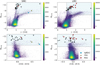 |
Fig. 1 CMDs for the SMC (left) and LMC (right). The background points are sources from the catalogues used for target selection (Yang et al. 2019, 2021). The colour bar indicates the number density of the stellar population. We show RSGs classified by Levesque et al. (2006) in black. Inverted grey triangles indicate contaminating objects that were observed (i.e. SMC4, SMC5, and LMC9). Our final sample is shown using the coloured symbols indicated by the legend. Top: M[3.6] vs. J − [3.6] CMD, highlighting the criteria used to select supergiant stars with the blue shaded region. In the panel on the right, seemingly only seven inverted red triangles are plotted, which is due to the nearly identical position of LMC1 and LMC5. Bottom: M[3.6] vs. [3.6]–[4.5] CMD to visually inspect the locations of the objects using IRAC bands. The numbers correspond to the object IDs of the verified supergiants. |
2.3 Data reduction
The spectroscopic data were reduced using the MagE Spectral Extractor (MASE; Bochanski et al. 2009). The MASE pipeline offers the full reduction process from raw data to a 1D spectrum, including bias subtraction, flat fielding, sky subtraction, cosmic ray removal, flux and wavelength calibration, and, finally, the extraction of the echelle orders to 1D spectra for all exposures.
After carefully transforming the wavelength units from vacuum to air wavelengths, which is required for spectral modelling, we merged the individual exposures using the median flux in every wavelength bin. The 1D echelle orders were then connected using linear weighting at overlapping wavelengths to assemble the full 1D spectrum.
Artificial bumps were present in the merged spectrum, caused by the small offset between orders. We corrected for this by scaling down the individual orders so that their relative fluxes matched at overlapping wavelength sections. Once the spectrum was cleaned for these bumps, we scaled the flux back up in units of absolute flux. The spectra were not corrected for tellurics. The S/N presented in the fourth column of Table 2 was derived by calculating the median S/N in small chunks of pseudo-continuum in the I band and serves as a general indicator of the spectral quality (S/N ≥ 50 in most cases).
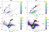 |
Fig. 2 Similar to Fig. 1, but for [24] vs. G − [24] (top) and G vs. GBP − Grp (bottom). The top CMD was used for the third selection criterion, while the bottom CMD was used to check whether the selected sources cluster in regions where they are expected. The RSG branch extends upwards in the middle, with the AGB branch extending to the right. |
Observational properties.
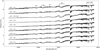 |
Fig. 3 Spectra from M-type sources in our sample (an arbitrary offset has been applied for illustration purposes). The Ca II triplet and key TiO bands are indicated. |
2.4 RV measurements
Before proceeding with the spectral modelling, the spectra were corrected for the radial velocity (RV) shift. Specifically, the Ca II triplet (λ8498, λ8542, λ8662), the Na I doublet (25890, 25896), and two resolved single metal lines close to the Ca II triplet (Ti I 28426 and Fe I 28612) were used to estimate the RV1. We measured the central wavelength for the selected metal lines by fitting a Gaussian to the line profile. Then, we calculated the offset from the rest wavelength for these lines to determine a velocity shift for each line profile. Precisely determined values for the rest wavelength of spectral lines were taken from the NIST atomic database (Kramida et al. 2020). The final RV was determined as the weighted mean of the shifts of individual lines. We then applied this RV shift to the spectrum. Towards mid-late M types, prominent metal lines disappear due to the increasing strength of TiO λ8432–8442–8452. In our sample this only applied to LMC2, for which we derived the velocity shift solely from the Ca II triplet. The mean RV for each target is presented in the sixth column of Table 2. We note that the RVs we have found are consistent with the systemic velocity of the LMC and SMC (260 km s−1 and 150 km s−1, respectively; McConnachie 2012; van der Marel & Kallivayalil 2014), confirming their membership to these systems. When an RV value from Gaia DR2 was available, we compared our results and confirmed them to be consistent. Additionally, the improved Gaia Early Data Release 3 parallax (Gaia Collaboration 2021) was inspected. We found the parallaxes of all objects, considering their errors and the systematic correction from Lindegren et al. (2021) to be consistent with zero, which is in turn consistent with the extragalactic origin of the sources.
2.5 Spectral classification
2.5.1 Classification of RSGs
The abundant presence of molecular bands in the optical is a clear indicator of late-type stars. Depending on the metal content of the star, the relative strengths of the molecular bands are typically used to determine the spectral subtype of M stars. Despite being derived from strong and abundant molecular bands, the optical classification of M0-M3 stars posed difficulties: the relative strengths of the TiO bands change only slightly in this range, while metal lines at ~8400–8800 Åremain unchanged due to their insensitivity to temperature (Solf 1978). For later types (M4–M6), Solf (1978) indicated the blending of the Ti II 28435 doublet with the triple TiO band head at λ8432–8442–8452 as the primary classifier.
Given these spectral classification criteria, we then proceeded with the classification of our spectra by visual inspection. Nine stars were identified as M-type stars due to the presence of strong molecular TiO bands at 26150 and 27050. Figure 3 presents the optical spectra of these stars. The most important spectral features are indicated, as is the spectral type. For seven of these stars, we identified similar TiO band strengths amongst them. For this group, we sorted the spectra from the weakest TiO 27050 band (M1) to the strongest (M3). Intermediate objects were classified as M2. The remaining two stars (LMC2 and LMC4) were noticeably different from the rest of the sample. Figure 4 highlights spectral lines in the Ca II triplet region, for example Ti II λ435. For LMC2, the TiO λ8432 band is present and blends with Ti II λ8435, but does not dominate the metal lines in this region. When the spectrum is depleted of metal line features due to the increasing TiO λ8432 band strength, the star is considered to be spectral type M6 (Negueruela et al. 2012). Therefore, we classified LMC2 as M4–5. For LMC4, the TiO bands at λ6150 and λ7050 were present but were noticeably weaker compared to the other stars, indicating an early M type. We classified this object as M0.
For the luminosity class, we used the strength of the Ca II triplet (λ8498, λ8542, λ8662) as the main criterion. The Ca II triplet is sensitive to changes in surface gravity due to pressure broadening, but insensitive to Teff and Z changes (Massey 1998). Therefore, a strong Ca II triplet is expected for supergiant stars. A strong Ca II triplet was indeed detected in all stars, with the exception of LMC2 (see Fig. 4). Apart from the Ca II triplet, the ratio between Fe I λ8514 and Ti I λ8518 was indicative of luminosity class I (except for LMC2, where neither line clearly dominates the other; Britavskiy et al. 2014). LMC2 was classified as M4–5 II–III as it does not satisfy the criteria to be classified as a luminosity class I star. To our knowledge, criteria for luminosity class II are not well established. Therefore, we cannot reject this possibility and present a range of luminosity class II-III for this object.
The variability types presented in Table 1 support the spectral classification, as semi-regular and slow-irregular types are often attributed to the RSG or red-giant class. Furthermore, most of our classified RSGs show minimum to modest variability in the optical (up to 1.5 magnitudes), which is expected for RSGs. The final classification of our objects, along with a comparison to older classifications and references, is presented in the final columns of Table 2.
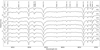 |
Fig. 4 Zoom in on the Ca II triplet and prominent metal lines (see Dorda et al. 2016) used for the classification of the objects and RV analysis. Features marked with an asterisk are blends and only the most significant line is indicated. For LMC2, Ti I λ8435 is relatively strong and the ratio between Fe I λ8514 and Ti I λ8518 line strengths is close to unity. |
2.5.2 Classification of other supergiants
During the observing campaign, two additional evolved massive stars were observed. We present spectra for them in Figs. 5, A.1, A.2, and A.3. The nature of their spectra was such that they could be classified but needed higher spectral resolution for adequate modelling (i.e. the models constrain properties from narrow metal line ratios), and this was not pursued. We briefly describe their spectral types here.
The spectrum of SMC1 displayed strong double-peaked emission for the Balmer series and several forbidden [O I] and [Fe II] emission lines (see Fig. A.1). These features originate from a circumstellar disk or ring structure (Maravelias et al. 2018). Despite being previously classified as a B8 I[e] (Zickgraf et al. 1992, spectrum taken in December 1989) and as an A1 I[e] (Kraus et al. 2008, spectrum taken in October 2000), we determined a spectral type of A0 I[e] (spectrum taken in December 2018) from the Mg II λ4481 to He I λ4471 line ratio (see Fig. A.2). If Mg II λ4481 ≥ He I λ4471, the spectral type is later than B9, while when the ratio of Ca K/(Hє+Ca H) ≤ 0.33, the spectral type is A0 (Evans et al. 2004), which is the case for our spectrum. We also note that the He I lines reappeared in our spectrum, after being absent in the spectrum analysed by Kraus et al. (2008), making the spectrum appear slightly hotter than it was in Kraus et al. (2008). Assuming the spectra have been classified correctly in past studies, the spectral type of SMC1 apparently varied on a scale of decades. For the RV measurement, several metal lines in the optical wavelength range were used, such as Mg II λ4481, He 1 λ4471,5875, Si II λ6347, and Fe II λ4174, 4179. Modelling of this source was not pursued due to the complexity of modelling the disk emission features and their contaminating effect on key Balmer and He I lines.
SMC2 is a YSG star that displayed a strong Hα emission component, indicating a mass-loss component surrounding the star. The spectrum is characterised by a series of Ti and Fe lines in the 4000–5000 Å region and strong Ca II H and K absorption (see Fig. A.3). We classified this star as F8 I due to the absence of the G band (< G0) and the strong Ti-Fe forest lines relative to the Balmer lines at Z = 0.2 Z⊙ (>F5). The sharpness of the Balmer lines and the strengths of the metal lines suggest that this star is of luminosity class I. For the RV, several resolved metal lines were used, such as Mg II λ4481, Si II λ6347, and Na I λ5890, 5896. For YSGs, spectral models are scarce. Models for a Teff estimate based on Fe line ratios have recently been published (Kourniotis et al. 2022); however, they require us to resolve narrow Fe lines. Our current spectrum is not able to resolve these lines, and therefore a higher resolution spectrum is needed to be able to derive a Teff empirically.
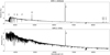 |
Fig. 5 Spectra of two additionally observed supergiants. Top: Spectrum of SMC1, an A0 I[e] star. The spectrum is characterised by several strong emission lines, which are indicated. Bottom: Spectrum of SMC2, an F8I star. Strong Hα emission was detected, indicating expanding circumstellar material. |
2.5.3 Classification of other sources
Three more objects fitting the selection criteria were observed (see Figs. 1 and 2, inverted grey triangles) but were not classified as evolved massive stars. Their spectra are presented in Fig. 6. We find SMC4 and SMC5 to have characteristic features of giant stars, while LMC9 shows the characteristics of an ionised nebula.
The spectrum of SMC4 contains carbon absorption bands at λ4737 and λ5165 and deep P-Cygni profiles indicative of strong mass loss (Whitelock et al. 1989), which could explain its extreme magnitude at [24]. SMC4 is a spectroscopic binary, with pairs of shifted spectral lines. We classified the primary star as a carbon star with moderately strong Swan C2 bands at λ4737 and λ5165, but with the absence of the C2 λ5585 band. Due to the strength of the Balmer lines, the absence of Ca I λ4426, and the presence of the G band, albeit weak compared to Hγ, we conclude this star to be a G type, and its carbon star equivalent should therefore be in the range C0–2. We were not able to obtain a more secure classification due to the contaminating features of the companion star.
SMC5 is characterised by extreme TiO absorption bands. The relative strengths of the TiO bands are indicative of a late M star, beyond M6. The strength of VO λ7900 suggests a spectral type of M7. The strength of the Ca II triplet indicates the star is of luminosity class III.
The spectrum of LMC9 was characterised by strong, narrow emission lines, most notably the [O III] feature at λ5007 and a saturated Hα emission component. Most of the emission lines were identified as recombination lines from low ionisation states, typically present in an HII region. A stellar continuum was observed underneath the sharp emission lines, revealing a bright blue object. From the broadened Balmer line profiles and Fe II emission lines present throughout the spectrum, we conclude that a luminous blue variable candidate (LBVc) may be present inside this HII region, although further investigation is needed to verify this object as such.
3 Spectral modelling and resulting parameters
3.1 Fitting the MARCS models
We used a grid of alpha-poor, spherical MARCS model atmospheres (Gustafsson et al. 2008) to fit the M-type stars in our sample. The computed models have a mass of 15 M⊙. Given the expected mass range for stars that evolve towards the RSG phase (8 M⊙ ≤ M* ≤ 25 M⊙) and the availability of models with limited discrete stellar masses (0.5, 1, 2, 5 and 15 M⊙), the 15 M⊙ model was the most suitable for our studies. Furthermore, we assume that a single mass to represent the entire range of masses for RSGs is justified given that the geometrical thickness, and thus the atmospheric structure, is largely unaffected in this mass range (Davies et al. 2010). The microturbulent velocity of the models was fixed to ξ = 5 km s−1. González-Torà et al. (2021) have shown that changes in ξ have little effect on the final result. We used MARCS models with log(Z/Z⊙) = −0.35 dex for the LMC and log(Z/Z⊙) = −0.55 dex for the SMC, which adequately represent the average metallicity derived empirically from a set of RSGs in the Magellanic Clouds (Davies et al. 2015). The surface gravities vary between −0.5 and +0.5 dex in steps of 0.1 dex. Only models with a surface gravity of +0.5, +0.0, and −0.5 dex were available from the MARCS platform, and hence we interpolated the flux of adjacent models linearly to make the grid denser. The effective temperature ranges from 3300–4500 K, in 10 K steps for the range 3300–4000 K and 25 K steps for the range 4000–4500 K using similar interpolation strategies.
We first degraded the resolution of the models from R = 20 000 to R = 4000 so that the model spectrum matched the spectral resolution of MagE. We then applied Fitzpatrick (1999) reddening laws with varying AV to the models to derive the best-fit extinction factor, assuming a typical total-to-selective extinction of RV = 2.74 and RV = 3.41 for the SMC and LMC, respectively (Gordon et al. 2003). We note that the values for RV may be higher, considering the grain size distribution in the circumstellar environment of RSGs (Massey et al. 2005). A recent study by González-Torà et al. (2021), however, indicates that changes in RV and the type of extinction law used do not largely contribute to temperature changes of the best-fit model. To obtain the best-fit model to our spectra, we computed the reduced chi-squared ( ):
):
 (1)
(1)
where v is the degrees of freedom, Fi and Fi,mod are the fluxes of the spectrum and model, respectively, and σi is the uncertainty on the flux in bin i. The degrees of freedom are set by the number of bins minus the number of free parameters (Teff and AV). The accepted best-fit model was the model on the 2D grid with the lowest  (i.e.
(i.e.  ). As in González-Torà et al. (2021), we chose to smooth the spectra to determine the
  , given that there may be uncertainties in the molecular transitions in the MARCS models. Bin-by-bin fitting of the single wavelength bins may therefore yield unrealistic
  , which could heavily impact the
  . For both the model and the observed spectrum, we grouped smaller wavelength bins into larger bins of 50 Å and set the mean flux of the new bin as the corresponding data point. We then calculated the
  of the larger bin using the mean flux and mean error (i.e. the standard deviation of the flux measurements). We fitted selected wavelength bins between 5400 Å and 8800 Å, which include the most prominent and temperature sensitive TiO bands as well as the bluest and reddest 100 Å to describe the slope of the spectrum to estimate AV. Upon inspecting the
  values after the initial run, we chose to discard the TiO band at 6150 Å from the calculation, as the molecular transitions in the models do not accurately match the features of real RSG spectra (see Fig. 7) and therefore skew the results. As our spectra were not corrected for telluric contamination, we avoided bins that included telluric bands. Isolated telluric lines may still be present (Catanzaro 1997), but given the use of the aforementioned smoothing technique, this does not significantly affect the
  calculation.
We approached the modelling as follows: we first fitted the Ca II triplet to derive the surface gravity (log g). The Ca II triplet is the primary diagnostic sensitive to the pressure broadening in the optical, so fitting this narrow spectral domain allowed us to get a precise measurement of the surface gravity. We proceeded by fixing the derived value of log g for the remainder of the fitting routine. We then fitted a 2D grid of models with variable AV and Teff to the spectrum and located the point on the grid with  . An example fit is presented in Fig. 7, in which we show the observed spectrum compared to the model (see Fig. A.4 for the remainder of the objects). From here on, we combine the extracted best-fit model parameters with photometry to derive the luminosity and subsequent radius of the star. For this, we used the K-band magnitude (mK), an appropriate bolometric correction for the K band based on the spectral type (Davies et al. 2018), and the distance modulus (µLMC = 18.477 ± 0.030 and µSMC = 18.95 ± 0.07 mag; Pietrzński et al. 2019; Graczyk et al. 2014) to derive Mbol (Mbol = mK − µ − AK+BCK). Using the magnitude-luminosity relation, we then derived L* (
 , with L0 being the zero point luminosity of the Sun, ~ 3 × 1028 W). The radius (R*) was derived from the Stefan-Boltzmann equation (
 ). The parameters corresponding to the best-fit model of each star (i.e.
  , Teff,TiO, AV, Mbol, log(L*/L⊙), and R*) are presented in Table 3.
To propagate the uncertainties, similar to Davies et al. (2010), we constructed a 2D χ2 map for all fitted stars (see Fig. 8).
The χ2 map shows the derived χ2 for every point on the 2D grid. Using  (where ∆χ2 = 2.3, 6.2, and 11.8 for 1, 2, and 3σ), we were able to derive uncertainties from the contours around the best-fit solution and take the extreme points as the inferred uncertainties. Following standard error propagation rules, we then estimated uncertainties for Mbol, log(L*/L⊙), and R*, which are listed in Table 3.
 |
Fig. 6 Spectra of three observed contaminants to our sample. Top: Spectrum of SMC4, a carbon star. The spectrum is characterised by two molecular carbon bands and several strong, deep P Cygni profiles. Middle: Spectrum of SMC5, a late M giant star. Strong TiO bands are revealed in the red part of the spectrum, indicating a low effective temperature. From the Ca II triplet, only λ8662 is present, albeit almost completely blended in with the overarching TiO band. Bottom: Spectrum of LMC9, an ionised nebula. The overall spectrum is dominated by strong emission lines coming from a nebula. Strong [O III] was detected, and the Hα emission was saturated. The emission line profile of Hα shows significant broadening, and other circumstellar lines (Fe II) were detected in the left wing of Hα, revealing an LBVc. |
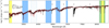 |
Fig. 7 Best MARCS model fit (dotted red line) to the spectrum of LMC1 (solid black line). Regions included in the |

Parameters derived for stars of spectral class M.
3.2 Comparison to Teff(J − K)
The effective temperature one derives depends on the region in the RSG atmosphere probed, resulting in systematic offsets between different methods. Numerous approaches have been developed in the last two decades to derive Teff for RSGs. Each of these approaches uses a different set of spectral or photometric features, so that depending on the data available, for both optical and near-IR wavelengths, methods have been established to derive Teff for RSGs. One approach is to convert photometric data into an effective temperature through empirical relations. As near-IR wavelengths are not very susceptible to extinction and variability (van Loon et al. 1999; Whitelock et al. 2003; Mauron & Josselin 2011), we opted to use the Teff(J − K) relations (Tabernero et al. 2018; Britavskiy et al. 2019a,b). These relations probe a temperature closer to the τλ = 2/3 continuum region, allowing us to discuss potential weaknesses of the TiO method as the molecular absorption happens in layers where τλ ≤ 2/3. Britavskiy et al. (2019a,b) fitted a sample of several hundred RSGs from Tabernero et al. (2018). In this study, Tabernero et al. (2018) derived effective temperatures from spectral lines in the 8400–8800 Å region by averaging the Teff derived from plane-parallel Kurucz models (Mészáros et al. 2012) and spherical MARCS models. Britavskiy et al. (2019a,b) then obtained a linear relation between the Teff and the (J − K) colour for both Magellanic Clouds. However, Teff (J − K) does not serve as a direct comparison to the Teff,TiO due to the nature of the derived spectroscopic Teff. A direct comparison could only be made if a relation between the J − K colours and the Teff,TiO were to be established in the future, or if one constructed a relation between the J − K colours and the temperature of the MARCS models, which will be attempted in a future work.
We used the relations presented in Britavskiy etal. (2019a,b), which are applicable for the LMC and SMC, respectively:
 (2)
(2)
 (3)
(3)
First we corrected for the reddening by calculating (J − Ks)0 from the relation (J − Ks)0 = (J − Ks) − E(J − K), where E(J − K) = 0.535E(B − V), (Schlegel et al. 1998) and  , with RV = 2.74 and RV = 3.41 for the SMC and LMC, respectively. Therefore, the reddening correction ultimately depends on the derived AV from Sect. 3.1. Although this affects the integrity of the comparison, as we used our derived AV to de-redden the independent J − K colour, using an independent AV (i.e. from an extinction map) would not affect the Teff(J − K) much (by ±50 K per 0.5 mag, which is arguably small compared to the adopted error of ±140 K). The resulting Teff(J − K) using Eqs. (2) and (3) are presented in the last column of Table 4. In most cases, Teff(J − K) is higher than Teff,TiO, as expected. It is noted that Eqs. (2) and (3) are valid in the range 0.8 ≤ J − Ks ≤ 1.4 mag; however, two of our objects had colours slightly beyond the upper limit, so we extrapolated the relations accordingly. Britavskiy et al. (2019a,b) indicated a typical error of ±140 K as the statistical uncertainty on their linear fit, which we adopted.
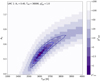 |
Fig. 8 Map of AV and Teff for LMC1, with darker shades indicating parts of the grid with lower χ2 values. The χ2 values of the colour bar are with respect to the minimum χ2. Contours at 1σ, 2σ, and 3σ are indicated to estimate the uncertainties. |
Spectroscopic and photometric Teff for the M supergiants.
4 Discussion
4.1 Hertzsprung–Russell diagram analysis
We used evolutionary models to verify the evolutionary status through the derived Teff and L of our stars. We used MIST models (Dotter 2016; Choi et al. 2016) for rotating stars (v/vcrit = 0.4) in the range 8 to 25 M⊙. We used the MIST models instead of the Geneva models as the former better reproduced the RSG population from Yang et al. (2021) at higher masses. The goal of this section is to provide a crude comparison of our sample to the tracks, not to derive properties. The tracks terminate at carbon core depletion, thus approaching the imminent collapse as a supernova and effectively mapping the entire evolution of a massive star from the main sequence to the final evolutionary stages.
We overlay evolutionary tracks on our data in Fig. 9. We also added sources from Levesque et al. (2006) and Davies et al. (2013), who presented similarly derived v results, allowing us to make a direct comparison between the two samples. We note that a considerable fraction of the RSGs lie in the forbidden zone of the evolutionary tracks, to the right of the Hayashi limit. We recall that the Teff of these points is determined from the TiO bands, while the Teff of the models probe the (hotter) continuum temperature. Indeed, when we construct a Hertzsprung–Russell diagram (HRD) using the Teff(J − K) approach (see Fig. 9, right panel), we see that the discrepancy becomes minimal and only a few outliers remain. Binary interactions cannot be used to explain the position in the HRD for these outliers. As the location of the RSGs in the HRD is largely unaffected by the amount of envelope mass of the RSGs, except for very low or very high envelope masses (Farrell et al. 2020; Beasor et al. 2020), it is difficult to infer these scenarios. For moderate envelope masses, an increase in envelope mass would make an object appear slightly hotter.
Most of our objects are in agreement with predictions from single star evolutionary tracks. We identified three potential outliers: LMC2, LMC3, and SMC3.
LMC2 (M4-5 II–III) is located at the lower luminosity end of the population compared to the RSGs studied in Levesque et al. (2006) and Davies et al. (2013). This is in agreement with the luminosity classification we have assigned. Using the derived Teff,TiO, it appears that LMC2 is too cool to be explained by any of the evolutionary tracks (see Fig. 9, left panel). This source is well within the range of tracks if we consider Teff(J − K), however (see the right panel of Fig. 9). Despite the spectral classification, and considering that the Teff(J − K) is closer to the real temperature of the photosphere, we find that the properties of this star are consistent with those of RSGs, which is in conflict with the spectral classification. It is possible, however, that there is a circumstellar contribution to the K–band magnitude that results in a higher luminosity.
LMC3 (M3 I) is brighter than other M-type supergiants. Since the star appears to be saturated in archival optical Hubble Space Telescope images, we could not find direct evidence of a contaminated K–band magnitude by an unresolved binary, which could potentially affect the derived luminosity. If this star is truly single, it may be grouped amongst the largest supergiants (R = 1390 R⊙) known in the LMC, albeit still trailing WOH G64 in size (R = 1540 R⊙, log(L*/L⊙) ~5.45; Levesque et al. 2009). Even though LMC3 is slightly brighter than WOH G64, we note that the luminosity of WOH G64 has been carefully corrected for contaminating contributions in the K–band magnitude, while LMC3 has not been. Further investigation is needed to carefully constrain the stellar radius and luminosity of LMC3 with more certainty. Considering the RSG sample of Davies et al. (2018), this object is at the high luminosity end of what has been observed and what is predicted by the Geneva models at Z = 0.006 from Eggenberger et al. (2021), indicating that this star is a high mass RSG at the latest stages of evolution.
SMC3 (M2 I) is one of the latest-type RSGs in the SMC and lies in the forbidden zone, as can be seen in the left panel of Fig. A.5. SMC3 does not cluster with the sources from similar studies and appears to be cooler and less luminous. However, if we employ a different methodology to derive the effective temperature (i.e. Teff(J − K); see the right panel of Fig. A.5), this source is not an outlier. We also note that if one considers the variability of the stars, LMC2 and SMC3 may not strictly be outliers.
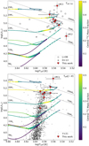 |
Fig. 9 Locations of the RSGs in the LMC compared to evolutionary tracks. Top: HRD with the locations of our LMC targets indicated with inverted red triangles. The Teff for all data points was derived through the TiO method. Smaller light grey squares and stars are objects from Levesque et al. (2006) and Davies et al. (2013), respectively. For the two outliers we have extended the uncertainty assuming a shift of 0.3 mag in the K band (dotted vertical error bar) instead of only the propagated uncertainty, to visualise the effect of intrinsic variability. The colour map represents the central 12C mass fraction, while the nodes on the track again indicate a step of 104 yr. Bottom: same as the top, but for Teff derived using the Teff(J − K) method. We show the general RSG population in the background (black points; Yang et al. 2021). |
4.2 Metallicity dependence
As stated in Sect. 3.1, we are guided by empirically derived metallicities from Davies et al. (2015, log(Z/Z⊙) = −0.35 dex for the LMC and log(Z/Z⊙) = −0.55 dex for the SMC RSG populations, respectively), and we proceeded with the spectral modelling using the most appropriate models available for these values. Given that (i) the models and empirical values are slightly different, (ii) we have fitted metal-dependent molecular bands, and (iii) the metallicity may not strictly be uniform within the Magellanic Clouds, we tested if the metallicity could possibly affect the results. We argue that the use of one single metallicity per galaxy is justified: (i) The general metallicity gradient ([Fe/H] abundance) in the SMC is flat and shows a small linear decrease outwards for the LMC (Cioni 2009). (ii) Davies et al. (2013) discussed small variations in metallicity not significantly affecting the results. Indeed, changing the value of log(Z/Z⊙) significantly (by ±0.25 dex) did not affect the effective temperature on a 50 K scale in their study, and is therefore not expected to affect our results much.
4.3 Teff,TiO − Teff(J−K) discrepancy
The Teff,TiO is generally systematically lower in comparison to continuum temperature methods (i.e. Teff(J − K) and the Teff derived through SED fitting) due to the region at which these TiO molecules are formed. Similar to Teff, the extinction, AV, is remarkably low. By selecting dusty, red sources in the CMDs presented in Sect. 2, we expected to find high extinction objects. Using this fitting method, however, we find extinction factors AV < 1, despite the fact that the extinction should be the sum of the contributions from foreground extinction, extinction from the star-forming region, and circumstellar extinction.
The SED method has been indicated by many authors as a more reliable method for extracting Teff compared to the TiO bands (Davies et al. 2013; González-Torà et al. 2021; Davies & Plez 2021). This is due to the fact that the TiO molecular absorption happens in a region where τλ ≠ 2/3, not near the photosphere. Here, we stress that we derived the Teff,TiO, not the true Teff of the RSG, which is technically defined to be at τλ = 2/3. Davies et al. (2013) extensively discuss MARCS models not correctly representing the radial temperature structure of a real RSG, as the line formation zone of the TiO bands is pushed to higher altitudes and lower temperatures. To fit the optical molecular bands properly, detailed 3D models that correctly take convection into account are needed. Davies et al. (2013) conclude that the temperature of the layer at which the continuum forms is consistent between the 1D and 3D models, and hence they argue that, for 1D models, using the continuum is more reliable. Finally, they suggest that the TiO method may be further hampered by the fact that TiO molecules may form in the wind region and that the TiO absorption strengths therefore also depend on the wind properties.
Some studies, however, provide opposing results. The recent study by Massey et al. (2021) suggested that Geneva single star (Eggenberger et al. 2008; Ekström et al. 2012) and BPASS binary (Stanway & Eldridge 2018) models fit observed RSG/WR (Wolf-Rayet; WR) ratios the best if the adopted effective temperature is the one derived through spectroscopy, not photometry (i.e. Teff(J − K)). They argue that using the spectroscopically derived Teff of stars yields a better match of their position in the HRD with respect to evolutionary tracks. However, Massey et al. (2021) also mention that it is uncertain whether the Teff adopted in the models can be interpreted as being equal to what is derived from a real RSG spectrum.
5 Summary and conclusions
We set out to find dusty, luminous evolved massive stars using near- and mid-IR selection criteria. We have spectroscopically confirmed eight new dusty, luminous RSGs, a new bright giant (LMC2), a new YSG (SMC2, with strong Hα emission), and three contaminants (i.e. two giants and an LBVc + HII region) through the analysis of newly obtained MagE spectra. In addition, we find a different spectral type for the sgB[e] star (SMC1, A0 I[e]) compared to the previous classifications reported in the literature (B8 I[e] and A1 I[e]), which suggests that this star has changed spectral type more than once over a 30-yr period, although we remain speculative over the physical mechanism that modifies the photosphere of the central star. The RSGs were analysed and modelled using the MARCS models to derive key properties. We approached the modelling by fitting the optical TiO bands to a precision of 50 K and used evolutionary tracks to determine the current evolutionary stage of these objects. We derived the physical properties of these RSGs. Most sources are very luminous (log(L*/L⊙) ≥ 5 dex) and have large radii (R* ~ 700–1400 R⊙). The brightest RSG (LMC3) appears disconnected from the bulk of the RSG population in the HRD. This object is located at the tail of the empirical and theoretical RSG luminosity distribution and is arguably one of the brightest and largest stars known in the LMC, with log(L*/L⊙) ~ 5.45 dex and R* ~ 1400 R⊙, resembling WOH G64 in size and luminosity (Levesque et al. 2009).
We have compared our results and methodology to other studies, computed the Teff(J − K) of our RSGs, and discussed the implications. The majority of our RSGs have a Teff,TiO that is arguably different from what is expected through Teff(J − K), although hotter temperatures are expected for Teff(J − K) as this temperature probes a deeper layer, closer to τλ ~ 2/3.
Despite the aim to select dusty supergiants, using the methodology as presented in this paper has resulted in lower extinction coefficients (AV < 1 mag) than expected. Davies et al. (2013) demonstrated that the derived extinction from the optical was in almost all cases much lower than that derived using the near-IR. We share their conclusion that using the optical TiO bands to derive the extinction is not ideal. We suggest the use of near-IR spectra or SED fitting for a more reliable result.
We conclude that the selection criteria were successful in selecting cool, luminous RSGs. However, in the near future we aim to apply the machine learning algorithm from Maravelias et al. (2022) to improve the selection of candidate evolved massive stars. The next step is to employ DUSTY models (Ivezic & Elitzur 1997) to derive mass-loss rates from the SED (e.g. Yang et al., in prep.). The derivation of the central star properties constrains the parameter space used with DUSTY. This significantly decreases the amount of viable models, which in turn reduces degeneracies and computation time. Finally, we emphasise that LMC3 is a remarkable source, and we aim to present a more detailed analysis of this star in a future study.
Acknowledgements
We thank the referee, Ben Davies, for the careful reading of the manuscript and the insightful comments and suggestions that significantly improved the manuscript. S.dW., A.Z.B., F.T., G.M., M.Y., E.Z. acknowledge funding support from the European Research Council (ERC) under the European Union’s Horizon 2020 research and innovation program (Grant agreement no. 772086). NB acknowledges support from the postdoctoral program (IPD-STEMA) of Liege University. EZ also acknowledges support by the Swiss National Science Foundation Professorship grant (project number PP00P2 176868; PI Tassos Fragos). This paper includes data gathered with the 6.5 m Magellan Telescopes located at Las Campanas Observatory, Chile. This research has made use of NASA’s Astrophysics Data System. This research has made use of the SIMBAD database, operated at CDS, Strasbourg, France. This research has made use of the VizieR catalogue access tool, CDS, Strasbourg, France.
Appendix A Supplementary figures
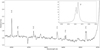 |
Fig. A.1 Prominent disk emission lines of SMC1 near the double-peaked Hα emission, which is shown in the inset at the top right. |
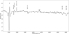 |
Fig. A.2 Zoom in on the metal lines used for the A0 I[e] spectral classification of SMC1. |
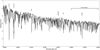 |
Fig. A.3 Zoom in on specific lines selected for the classification for SMC2 (spectral type F8 I). Balmer lines are moderately strong, metal lines are abundant, and the G band is weak. |
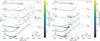 |
Fig. A.5 Locations of the RSGs in the SMC compared to evolutionary tracks. Left: Same as the top panel of Fig. 9 but for the SMC. Right: Same as the bottom panel of Fig. 9 but showing the general SMC RSG population from Yang et al. (2020) in the background. |
References
- Beasor, E. R., Davies, B., Smith, N., et al. 2020, MNRAS, 492, 5994 [Google Scholar]
- Beasor, E. R., Davies, B., & Smith, N. 2021, ApJ, 922, 55 [NASA ADS] [CrossRef] [Google Scholar]
- Bochanski, J. J., Hennawi, J. F., Simcoe, R. A., et al. 2009, PASP, 121, 1409 [NASA ADS] [CrossRef] [Google Scholar]
- Bonanos, A. Z., Massa, D. L., Sewilo, M., et al. 2009, AJ, 138, 1003 [Google Scholar]
- Bonanos, A. Z., Lennon, D. J., Köhlinger, F., et al. 2010, AJ, 140, 416 [NASA ADS] [CrossRef] [Google Scholar]
- Britavskiy, N. E., Bonanos, A. Z., Mehner, A., et al. 2014, A&A, 562, A75 [NASA ADS] [CrossRef] [EDP Sciences] [Google Scholar]
- Britavskiy, N., Lennon, D. J., Patrick, L. R., et al. 2019a, A&A, 624, A128 [NASA ADS] [CrossRef] [EDP Sciences] [Google Scholar]
- Britavskiy, N. E., Bonanos, A. Z., Herrero, A., et al. 2019b, A&A, 631, A95 [NASA ADS] [CrossRef] [EDP Sciences] [Google Scholar]
- Brott, I., de Mink, S. E., Cantiello, M., et al. 2011, A&A, 530, A115 [NASA ADS] [CrossRef] [EDP Sciences] [Google Scholar]
- Bruch, R. J., Gal-Yam, A., Schulze, S., et al. 2021, ApJ, 912, 46 [NASA ADS] [CrossRef] [Google Scholar]
- Catanzaro, G. 1997, Ap&SS, 257, 161 [NASA ADS] [CrossRef] [Google Scholar]
- Chen, R., Luo, A., Liu, J., & Jiang, B. 2016, AJ, 151, 146 [NASA ADS] [CrossRef] [Google Scholar]
- Choi, J., Dotter, A., Conroy, C., et al. 2016, ApJ, 823, 102 [Google Scholar]
- Cioni, M. R. L. 2009, A&A, 506, 1137 [NASA ADS] [CrossRef] [EDP Sciences] [Google Scholar]
- Cutri, R. M., Skrutskie, M. F., van Dyk, S., et al. 2003, VizieR Online Data Catalog: II/246 [Google Scholar]
- Davies, B., & Beasor, E. R. 2020, MNRAS, 493, 468 [NASA ADS] [CrossRef] [Google Scholar]
- Davies, B., & Plez, B. 2021, MNRAS, 508, 5757 [NASA ADS] [CrossRef] [Google Scholar]
- Davies, B., Kudritzki, R.-P., & Figer, D. F. 2010, MNRAS, 407, 1203 [NASA ADS] [CrossRef] [Google Scholar]
- Davies, B., Kudritzki, R.-P., Plez, B., et al. 2013, ApJ, 767, 3 [Google Scholar]
- Davies, B., Kudritzki, R.-P., Gazak, Z., et al. 2015, ApJ, 806, 21 [NASA ADS] [CrossRef] [Google Scholar]
- Davies, B., Crowther, P. A., & Beasor, E. R. 2018, MNRAS, 478, 3138 [NASA ADS] [CrossRef] [Google Scholar]
- de Jager, C., Nieuwenhuijzen, H., & van der Hucht, K. A. 1988, A&AS, 72, 259 [NASA ADS] [Google Scholar]
- Dorda, R., González-Fernández, C., & Negueruela, I. 2016, A&A, 595, A105 [NASA ADS] [CrossRef] [EDP Sciences] [Google Scholar]
- Dotter, A. 2016, ApJS, 222, 8 [Google Scholar]
- Egan, M. P., Van Dyk, S. D., & Price, S. D. 2001, AJ, 122, 1844 [NASA ADS] [CrossRef] [Google Scholar]
- Eggenberger, P., Meynet, G., Maeder, A., et al. 2008, Ap&SS, 316, 43 [Google Scholar]
- Eggenberger, P., Ekström, S., Georgy, C., et al. 2021, A&A, 652, A137 [NASA ADS] [CrossRef] [EDP Sciences] [Google Scholar]
- Ekström, S., Georgy, C., Eggenberger, P., et al. 2012, A&A, 537, A146 [Google Scholar]
- Eldridge, J. J., Fraser, M., Smartt, S. J., Maund, J. R., & Crockett, R. M. 2013, MNRAS, 436, 774 [NASA ADS] [CrossRef] [Google Scholar]
- Evans, C. J., Howarth, I. D., Irwin, M. J., Burnley, A. W., & Harries, T. J. 2004, MNRAS, 353, 601 [NASA ADS] [CrossRef] [Google Scholar]
- Farrell, E. J., Groh, J. H., Meynet, G., & Eldridge, J. J. 2020, MNRAS, 494, L53 [NASA ADS] [CrossRef] [Google Scholar]
- Fazio, G. G., Hora, J. L., Allen, L. E., et al. 2004, ApJS, 154, 10 [Google Scholar]
- Fitzpatrick, E. L. 1999, PASP, 111, 63 [Google Scholar]
- Gaia Collaboration (Prusti, T., et al.) 2016, A&A, 595, A1 [NASA ADS] [CrossRef] [EDP Sciences] [Google Scholar]
- Gaia Collaboration (Brown, A. G. A., et al.) 2018, A&A, 616, A1 [NASA ADS] [CrossRef] [EDP Sciences] [Google Scholar]
- Gaia Collaboration (Brown, A. G. A., et al.) 2021, A&A, 649, A1 [NASA ADS] [CrossRef] [EDP Sciences] [Google Scholar]
- Goldman, S. R., van Loon, J. T., Zijlstra, A. A., et al. 2017, MNRAS, 465, 403 [Google Scholar]
- González-Torà, G., Davies, B., Kudritzki, R.-P., & Plez, B. 2021, MNRAS, 505, 4422 [CrossRef] [Google Scholar]
- Gordon, K. D., Clayton, G. C., Misselt, K. A., Landolt, A. U., & Wolff, M. J. 2003, ApJ, 594, 279 [NASA ADS] [CrossRef] [Google Scholar]
- Graczyk, D., Pietrzynski, G., Thompson, I. B., et al. 2014, ApJ, 780, 59 [Google Scholar]
- Groenewegen, M. A. T., & Blommaert, J. A. D. L. 1998, A&A, 332, 25 [NASA ADS] [Google Scholar]
- Groenewegen, M. A. T., & Sloan, G. C. 2018, A&A, 609, A114 [NASA ADS] [CrossRef] [EDP Sciences] [Google Scholar]
- Gustafsson, B., Edvardsson, B., Eriksson, K., et al. 2008, A&A, 486, 951 [NASA ADS] [CrossRef] [EDP Sciences] [Google Scholar]
- Humphreys, R. M., & Jones, T. J. 2022, AJ, 163, 103 [NASA ADS] [CrossRef] [Google Scholar]
- Ivezic, Z., & Elitzur, M. 1997, MNRAS, 287, 799 [Google Scholar]
- Jayasinghe, T., Kochanek, C. S., Stanek, K. Z., et al. 2018, MNRAS, 477, 3145 [Google Scholar]
- Jones, O. C., Woods, P. M., Kemper, F., et al. 2017, MNRAS, 470, 3250 [NASA ADS] [CrossRef] [Google Scholar]
- Köhler, K., Langer, N., de Koter, A., et al. 2015, A&A, 573, A71 [NASA ADS] [CrossRef] [EDP Sciences] [Google Scholar]
- Kourniotis, M., Kraus, M., Maryeva, O., Borges Fernandes, M., & Maravelias, G. 2022, MNRAS, 511, 4360 [NASA ADS] [CrossRef] [Google Scholar]
- Kramida, A., Yu. Ralchenko, Reader, J., & NIST ASD Team 2020, NIST Atomic Spectra Database (ver. 5.8), [Online] Available: https://physics.nist.gov/asd [2017, April 9], National Institute of Standards and Technology, Gaithersburg, MD. [Google Scholar]
- Kraus, M. 2019, Galaxies, 7, 83 [NASA ADS] [CrossRef] [Google Scholar]
- Kraus, M., Borges Fernandes, M., Kubát, J., & de Araújo, F. X. 2008, A&A, 487, 697 [NASA ADS] [CrossRef] [EDP Sciences] [Google Scholar]
- Levesque, E. M. 2017, Astrophysics of Red Supergiants (IOP Publishing) [Google Scholar]
- Levesque, E. M., Massey, P., Olsen, K. A. G., et al. 2005, ApJ, 628, 973 [Google Scholar]
- Levesque, E. M., Massey, P., Olsen, K. A. G., et al. 2006, ApJ, 645, 1102 [NASA ADS] [CrossRef] [Google Scholar]
- Levesque, E. M., Massey, P., Plez, B., & Olsen, K. A. G. 2009, AJ, 137, 4744 [NASA ADS] [CrossRef] [Google Scholar]
- Lindegren, L., Bastian, U., Biermann, M., et al. 2021, A&A, 649, A4 [EDP Sciences] [Google Scholar]
- Maravelias, G., Kraus, M., Cidale, L. S., et al. 2018, MNRAS, 480, 320 [CrossRef] [Google Scholar]
- Maravelias, G., Bonanos, A. Z., Tramper, F., et al. 2022, A&A, 666, A122 [NASA ADS] [CrossRef] [EDP Sciences] [Google Scholar]
- Marshall, J. L., Burles, S., Thompson, I. B., et al. 2008, SPIE Conf. Ser., 7014, 701454 [NASA ADS] [Google Scholar]
- Massey, P. 1998, ApJ, 501, 153 [Google Scholar]
- Massey, P., Plez, B., Levesque, E. M., et al. 2005, ApJ, 634, 1286 [NASA ADS] [CrossRef] [Google Scholar]
- Massey, P., Neugent, K. F., Dorn-Wallenstein, T. Z., et al. 2021, ApJ, 922, 177 [NASA ADS] [CrossRef] [Google Scholar]
- Mauerhan, J. C., Smith, N., Filippenko, A. V., et al. 2013, MNRAS, 430, 1801 [NASA ADS] [CrossRef] [Google Scholar]
- Mauron, N., & Josselin, E. 2011, A&A, 526, A156 [CrossRef] [EDP Sciences] [Google Scholar]
- McConnachie, A. W. 2012, AJ, 144, 4 [Google Scholar]
- Mészáros, S., Allende Prieto, C., Edvardsson, B., et al. 2012, AJ, 144, 120 [Google Scholar]
- Negueruela, I., Marco, A., González-Fernández, C., et al. 2012, A&A, 547, A15 [NASA ADS] [CrossRef] [EDP Sciences] [Google Scholar]
- Pietrzynski, G., Graczyk, D., Gallenne, A., et al. 2019, Nature, 567, 200 [NASA ADS] [CrossRef] [Google Scholar]
- Podsiadlowski, P., Joss, P. C., & Hsu, J. J. L. 1992, ApJ, 391, 246 [Google Scholar]
- Prieto, J. L., Kistler, M. D., Thompson, T. A., et al. 2008, ApJ, 681, L9 [NASA ADS] [CrossRef] [Google Scholar]
- Reid, N., Tinney, C., & Mould, J. 1990, ApJ, 348, 98 [NASA ADS] [CrossRef] [Google Scholar]
- Rieke, G. H., Young, E. T., Engelbracht, C. W., et al. 2004, ApJS, 154, 25 [Google Scholar]
- Samus’, N. N., Kazarovets, E. V., Durlevich, O. V., Kireeva, N. N., & Pastukhova, E. N. 2017, Astron. Rep., 61, 80 [Google Scholar]
- Sanduleak, N. 1989, AJ, 98, 825 [NASA ADS] [CrossRef] [Google Scholar]
- Schlegel, D. J., Finkbeiner, D. P., & Davis, M. 1998, ApJ, 500, 525 [Google Scholar]
- Seale, J. P., Looney, L. W., Chu, Y.-H., et al. 2009, ApJ, 699, 150 [NASA ADS] [CrossRef] [Google Scholar]
- Shappee, B. J., Prieto, J. L., Grupe, D., et al. 2014, ApJ, 788, 48 [Google Scholar]
- Skrutskie, M. F., Cutri, R. M., Stiening, R., et al. 2006, AJ, 131, 1163 [NASA ADS] [CrossRef] [Google Scholar]
- Smartt, S. J. 2015, PASA, 32, e016 [NASA ADS] [CrossRef] [Google Scholar]
- Smartt, S. J., Eldridge, J. J., Crockett, R. M., & Maund, J. R. 2009, MNRAS, 395, 1409 [CrossRef] [Google Scholar]
- Smith, N. 2014, ARA&A, 52, 487 [NASA ADS] [CrossRef] [Google Scholar]
- Smith, N., Hinkle, K. H., & Ryde, N. 2009, AJ, 137, 3558 [NASA ADS] [CrossRef] [Google Scholar]
- Solf, J. 1978, A&AS, 34, 409 [Google Scholar]
- Stanway, E. R., & Eldridge, J. J. 2018, MNRAS, 479, 75 [NASA ADS] [CrossRef] [Google Scholar]
- Tabernero, H. M., Dorda, R., Negueruela, I., & González-Fernández, C. 2018, MNRAS, 476, 3106 [NASA ADS] [CrossRef] [Google Scholar]
- van der Marel, R. P., & Kallivayalil, N. 2014, ApJ, 781, 121 [Google Scholar]
- van Loon, J. T., Groenewegen, M. A. T., de Koter, A., et al. 1999, A&A, 351, 559 [NASA ADS] [Google Scholar]
- van Loon, J. T., Cioni, M. R. L., Zijlstra, A. A., & Loup, C. 2005, A&A, 438, 273 [NASA ADS] [CrossRef] [EDP Sciences] [Google Scholar]
- Werner, M. W., Roellig, T. L., Low, F. J., et al. 2004, ApJS, 154, 1 [NASA ADS] [CrossRef] [Google Scholar]
- Westerlund, B. E., Olander, N., & Hedin, B. 1981, A&AS, 43, 267 [NASA ADS] [Google Scholar]
- Whitelock, P. A., Feast, M. W., Menzies, J. W., & Catchpole, R. M. 1989, MNRAS, 238, 769 [CrossRef] [Google Scholar]
- Whitelock, P. A., Feast, M. W., van Loon, J. T., & Zijlstra, A. A. 2003, MNRAS, 342, 86 [NASA ADS] [CrossRef] [Google Scholar]
- Wood, P. R., Bessell, M. S., & Fox, M. W. 1983, ApJ, 272, 99 [Google Scholar]
- Yang, M., Bonanos, A. Z., Jiang, B.-W., et al. 2019, A&A, 629, A91 [NASA ADS] [CrossRef] [EDP Sciences] [Google Scholar]
- Yang, M., Bonanos, A. Z., Jiang, B.-W., et al. 2020, A&A, 639, A116 [NASA ADS] [CrossRef] [EDP Sciences] [Google Scholar]
- Yang, M., Bonanos, A. Z., Jiang, B., et al. 2021, A&A, 646, A141 [EDP Sciences] [Google Scholar]
- Zapartas, E., de Mink, S. E., Van Dyk, S. D., et al. 2017, ApJ, 842, 125 [CrossRef] [Google Scholar]
- Zickgraf, F. J., Stahl, O., & Wolf, B. 1992, A&A, 260, 205 [NASA ADS] [Google Scholar]
See Table C.1 in Dorda et al. (2016) for a complete atlas of spectral lines for cool supergiants in the i and z bands.
All Tables
All Figures
|
Fig. 1 CMDs for the SMC (left) and LMC (right). The background points are sources from the catalogues used for target selection (Yang et al. 2019, 2021). The colour bar indicates the number density of the stellar population. We show RSGs classified by Levesque et al. (2006) in black. Inverted grey triangles indicate contaminating objects that were observed (i.e. SMC4, SMC5, and LMC9). Our final sample is shown using the coloured symbols indicated by the legend. Top: M[3.6] vs. J − [3.6] CMD, highlighting the criteria used to select supergiant stars with the blue shaded region. In the panel on the right, seemingly only seven inverted red triangles are plotted, which is due to the nearly identical position of LMC1 and LMC5. Bottom: M[3.6] vs. [3.6]–[4.5] CMD to visually inspect the locations of the objects using IRAC bands. The numbers correspond to the object IDs of the verified supergiants. |
| In the text | |
|
Fig. 2 Similar to Fig. 1, but for [24] vs. G − [24] (top) and G vs. GBP − Grp (bottom). The top CMD was used for the third selection criterion, while the bottom CMD was used to check whether the selected sources cluster in regions where they are expected. The RSG branch extends upwards in the middle, with the AGB branch extending to the right. |
| In the text | |
|
Fig. 3 Spectra from M-type sources in our sample (an arbitrary offset has been applied for illustration purposes). The Ca II triplet and key TiO bands are indicated. |
| In the text | |
|
Fig. 4 Zoom in on the Ca II triplet and prominent metal lines (see Dorda et al. 2016) used for the classification of the objects and RV analysis. Features marked with an asterisk are blends and only the most significant line is indicated. For LMC2, Ti I λ8435 is relatively strong and the ratio between Fe I λ8514 and Ti I λ8518 line strengths is close to unity. |
| In the text | |
|
Fig. 5 Spectra of two additionally observed supergiants. Top: Spectrum of SMC1, an A0 I[e] star. The spectrum is characterised by several strong emission lines, which are indicated. Bottom: Spectrum of SMC2, an F8I star. Strong Hα emission was detected, indicating expanding circumstellar material. |
| In the text | |
|
Fig. 6 Spectra of three observed contaminants to our sample. Top: Spectrum of SMC4, a carbon star. The spectrum is characterised by two molecular carbon bands and several strong, deep P Cygni profiles. Middle: Spectrum of SMC5, a late M giant star. Strong TiO bands are revealed in the red part of the spectrum, indicating a low effective temperature. From the Ca II triplet, only λ8662 is present, albeit almost completely blended in with the overarching TiO band. Bottom: Spectrum of LMC9, an ionised nebula. The overall spectrum is dominated by strong emission lines coming from a nebula. Strong [O III] was detected, and the Hα emission was saturated. The emission line profile of Hα shows significant broadening, and other circumstellar lines (Fe II) were detected in the left wing of Hα, revealing an LBVc. |
| In the text | |
|
Fig. 7 Best MARCS model fit (dotted red line) to the spectrum of LMC1 (solid black line). Regions included in the |
| In the text | |
|
Fig. 8 Map of AV and Teff for LMC1, with darker shades indicating parts of the grid with lower χ2 values. The χ2 values of the colour bar are with respect to the minimum χ2. Contours at 1σ, 2σ, and 3σ are indicated to estimate the uncertainties. |
| In the text | |
|
Fig. 9 Locations of the RSGs in the LMC compared to evolutionary tracks. Top: HRD with the locations of our LMC targets indicated with inverted red triangles. The Teff for all data points was derived through the TiO method. Smaller light grey squares and stars are objects from Levesque et al. (2006) and Davies et al. (2013), respectively. For the two outliers we have extended the uncertainty assuming a shift of 0.3 mag in the K band (dotted vertical error bar) instead of only the propagated uncertainty, to visualise the effect of intrinsic variability. The colour map represents the central 12C mass fraction, while the nodes on the track again indicate a step of 104 yr. Bottom: same as the top, but for Teff derived using the Teff(J − K) method. We show the general RSG population in the background (black points; Yang et al. 2021). |
| In the text | |
|
Fig. A.1 Prominent disk emission lines of SMC1 near the double-peaked Hα emission, which is shown in the inset at the top right. |
| In the text | |
|
Fig. A.2 Zoom in on the metal lines used for the A0 I[e] spectral classification of SMC1. |
| In the text | |
|
Fig. A.3 Zoom in on specific lines selected for the classification for SMC2 (spectral type F8 I). Balmer lines are moderately strong, metal lines are abundant, and the G band is weak. |
| In the text | |
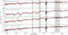 |
Fig. A.4 Same as Fig. 7, but for SMC3 and LMC2-8. |
| In the text | |
|
Fig. A.5 Locations of the RSGs in the SMC compared to evolutionary tracks. Left: Same as the top panel of Fig. 9 but for the SMC. Right: Same as the bottom panel of Fig. 9 but showing the general SMC RSG population from Yang et al. (2020) in the background. |
| In the text | |
Current usage metrics show cumulative count of Article Views (full-text article views including HTML views, PDF and ePub downloads, according to the available data) and Abstracts Views on Vision4Press platform.
Data correspond to usage on the plateform after 2015. The current usage metrics is available 48-96 hours after online publication and is updated daily on week days.
Initial download of the metrics may take a while.