| Issue |
A&A
Volume 686, June 2024
|
|
|---|---|---|
| Article Number | L9 | |
| Number of page(s) | 17 | |
| Section | Letters to the Editor | |
| DOI | https://doi.org/10.1051/0004-6361/202349088 | |
| Published online | 04 June 2024 | |
Letter to the Editor
A fading radius valley towards M dwarfs, a persistent density valley across stellar types⋆
1
Department of Astronomy, University of Geneva, Chemin Pegasi 51, 1290 Versoix, Switzerland
e-mail: This email address is being protected from spambots. You need JavaScript enabled to view it.
2
Instituto de Astrofísica de La Plata, CCT La Plata-CONICET-UNLP, Paseo del Bosque S/N (1900), La Plata, Argentina
3
Department of Space Research & Planetary Sciences, University of Bern, Gesellschaftsstrasse 6, 3012 Bern, Switzerland
4
Núcleo Milenio de Formación Planetaria (NPF), Valparaiso, Chile
Received:
22
December
2023
Accepted:
23
March
2024
Abstract
The radius valley separating super-Earths from mini-Neptunes is a fundamental benchmark for theories of planet formation and evolution. Observations show that the location of the radius valley decreases with decreasing stellar mass and with increasing orbital period. Here, we build on our previous pebble-based formation model. Combined with photoevaporation after disc dispersal, it has allowed us to unveil the radius valley as a separator between rocky and water-worlds. In this study, we expand our model for a range of stellar masses spanning from 0.1 to 1.5 M⊙. We find that the location of the radius valley is well described by a power-law in stellar mass as Rvalley = 1.8197 M⋆0.14(+0.02/−0.01), which is in excellent agreement with observations. We also find very good agreement with the dependence of the radius valley on orbital period, both for FGK and M dwarfs. Additionally, we note that the radius valley gets filled towards low stellar masses, particularly at 0.1–0.4 M⊙, yielding a rather flat slope in Rvalley − Porb. This is the result of orbital migration occurring at lower planet mass for less massive stars, which allows for low-mass water-worlds to reach the inner regions of the system, blurring the separation in mass (and size) between rocky and water worlds. Furthermore, we find that for planetary equilibrium temperatures above 400 K, the water in the volatile layer exists fully in the form of steam, puffing the planet radius up (as compared to the radii of condensed-water worlds). This produces an increase in planet radii of ∼30% at 1 M⊕ and of ∼15% at 5 M⊕ compared to condensed-water worlds. As with Sun-like stars, we find that pebble accretion leaves its imprint on the overall exoplanet population as a depletion of planets with intermediate compositions (i.e. water mass fractions of ∼0 − 20%), carving an planet-depleted diagonal band in the mass-radius (MR) diagrams. This band is better visualised when plotting the planet’s mean density in terms of an Earth-like composition. This change in coordinates causes the valley to emerge for all the stellar mass cases.
Key words: planets and satellites: atmospheres / planets and satellites: composition / planets and satellites: formation / planets and satellites: physical evolution
The data to generate the figures is available on Zenodo, https://doi.org/10.5281/zenodo.10719523
© The Authors 2024
 Open Access article, published by EDP Sciences, under the terms of the Creative Commons Attribution License (https://creativecommons.org/licenses/by/4.0), which permits unrestricted use, distribution, and reproduction in any medium, provided the original work is properly cited.
This article is published in open access under the Subscribe to Open model. This email address is being protected from spambots. You need JavaScript enabled to view it. to support open access publication.
1. Introduction
Exoplanets with sizes between Earth and Neptune are the most abundant type known until now (e.g. Petigura et al. 2022). The size distribution of these objects is bimodal, with a “radius valley” present at ∼1.5 − 2 R⊕ separating the smaller super-Earths from the larger mini- (or sub-)Neptunes (Fulton et al. 2017; Fulton & Petigura 2018; Van Eylen et al. 2018; Martinez et al. 2019). The exact location of the radius valley depends on the stellar mass and planets’ orbital period, with different data analysis yielding different slopes in the log(RP)−log(M⋆) and log(RP)−log(Porb) planes (with RP, Porb, and M⋆ as the planet radius, orbital period, and stellar mass, respectively; Fulton et al. 2017; Fulton & Petigura 2018; Berger et al. 2020; Petigura et al. 2022; Luque & Pallé 2022; Ho & Van Eylen 2023; Bonfanti et al. 2024).
Understanding the origin of the radius valley and its dependence on orbital and physical parameters has become a crucial endeavour in modern exoplanetology (e.g. Owen & Wu 2017; Ginzburg et al. 2018; Gupta & Schlichting 2019; Venturini et al. 2020a; Lee & Connors 2021). The first mechanisms to account for the existence of the radius valley were the pure evolution models known as photoevaporation (e.g Lopez & Fortney 2013; Chen & Rogers 2016; Owen & Wu 2017; Jin & Mordasini 2018) and core-powered mass-loss (Ginzburg et al. 2018; Gupta & Schlichting 2019). Based on these models, super-Earths and mini-Neptunes would originate from the same single-composition population of rocky cores with H/He atmospheres. The distinction between super-Earths and mini-Neptunes arises because some planets lose their atmospheres completely during the evolution, while others retain ∼1% by mass in terms of H/He. Both models find slopes in the radius-period and radius-stellar mass plane in agreement with observations (Gupta & Schlichting 2019; Rogers et al. 2021). However, these pure evolution models are in contradiction with planet formation theory, which predicts most mini-Neptunes to have formed beyond the water ic line and to therefore be water-rich (Alibert et al. 2013; Raymond et al. 2018; Bitsch et al. 2018; Izidoro et al. 2021; Brügger et al. 2020; Venturini et al. 2020a). In Venturini et al. (2020a, hereafter V20), we performed pebble-based planet formation simulations for Sun-like stars, including a self-consistent treatment of pebble growth. We found that because of the different physical properties of icy versus rocky pebbles, icy cores are typically born bigger than rocky ones. In terms of total planet radius, this bi-modality is hidden at the time of disc dissipation because most planets accrete gas that puffs the planetary radii up. The separation between rocky and water-worlds becomes clear once atmospheric mass-loss sets in, stripping the atmospheres of the small rocky and icy planets and unveiling the primordial radius valley separating the two planetary types, at ∼1.5–2 R⊕ (Venturini et al. 2020a). In this work, we adapt and apply our planet formation and evolution model to a wide range of stellar masses, from 0.1 to 1.5 M⊙ (i.e. stellar spectral types spanning M dwarfs to A types). The upper limit on stellar mass is motivated by the earliest-stellar-type exoplanets discovered by Kepler (e.g. Berger et al. 2020). On the theoretical side, we note that no population study has addressed the origin of planets orbiting super-solar stellar masses until now. This is important to address given the new TESS data on exoplanets around F and A stars (Psaridi et al. 2022).
Regarding M planets, the motivation to study them is based on the increasing number of facilities targeting such objects, such as TESS (Ricker et al. 2015), CHEOPS (Benz et al. 2021), and NIRPS (Bouchy et al. 2022). In particular, regarding the radius valley, several studies are reporting masses and radii of super-Earths and mini-Neptunes (e.g. Demory et al. 2020; Van Eylen et al. 2021; Luque & Pallé 2022; Bonfanti et al. 2024), and the mere existence of the radius valley for M dwarfs remains controversial (Cloutier & Menou 2020; Luque & Pallé 2022; Bonfanti et al. 2024). From a theoretical perspective, Alibert (2017), Miguel et al. (2020), and Burn et al. (2021) showed that low-mass water-rich planets are expected to be common at close-in orbits around M dwarfs.
In this work, we conduct a large planet formation and evolution parameter study, focusing on the population of low- and intermediate-mass planets. The aim is to devise a theoretical description of the behaviour of the radius valley for different stellar types. Our main results are highlighted in the brief main text, supplemented by several in-depth analysis in the Appendices.
2. Methods
We computed the formation and evolution of planets around stars of mass 0.1, 0.4, 0.7, 1.0, 1.3, and 1.5 M⊙. In our model (Venturini et al. 2020a,b), planets grow from a lunar-mass embryo by pebble and gas accretion, while embedded in a gaseous disc that evolves by viscous accretion and X-ray photoevaporation from the central star. The discs are adapted to different stellar masses following Burn et al. (2021) (details in Appendix A.1). The evolution of the pebbles was calculated considering pebble coagulation, fragmentation, drift, diffusion, and ice sublimation at the water ice line (model of Birnstiel et al. 2011; Drążkowska et al. 2016). The planets can accrete either rocky or icy pebbles, depending on its position with respect to the water ice line (which evolves in time, moving inwards as the disc cools down). Core growth halts when pebble isolation mass is reached (Lambrechts et al. 2014). As in V20, we adopted a fragmentation threshold velocity of icy and silicate pebbles as vth = 10 m s−1 and vth = 1 m s−1, respectively (e.g. Gundlach & Blum 2015). We note, based on experimental works, that these values are still quite uncertain (see detailed discussion in Appendix C.1.2). Our results hold as long as the fragmentation threshold velocity of icy pebbles is in the range of 5–10 m s−1. More experimental work and sensitivity studies are required to better constrain these fragmentation velocities. For the disc viscosity, we consider α to either be 10−3 or 10−4. The details about the choice of the initial conditions are given in Appendix A.1. The planets also migrate along the disc, either via the type I-or type-II regime. The former includes the Lindblad, corotation, and thermal torques (Guilera et al. 2019).
As explained in V20, since our code can handle at the moment the formation of only one embryo per disc, and given the fast timescales of pebble accretion and type-I migration, most of our formed planets get stranded near the disc inner edge, which is set at an orbital period of 11.55 days for all the considered discs (stemming from the choice of disc inner edge at 0.1 au for solar-type stars, see Appendix A.1). This means that most of the results reported throughout this work refer to planets with orbital period of ∼11–18 days.
Because of the limitation of considering only one embryo per disc, the possibility of atmospheric mass loss due to giant impacts is in principle hindered in our model. Nevertheless, as in V20, we estimated this rate in a simplified way, following Inamdar & Schlichting (2015) and Ronco et al. (2017), by considering a potential impact between the simulated planet and another, less massive one formed in a different simulation, but under the same disc initial conditions (see Appendix A.1). We refer to this batch of simulations as the “collision case” (while the standard simulations without the estimation of atmospheric mass-loss by collisions is referred as “nominal case”). The details of this implementation and its limitations can be found in Appendix A.3.
Once the disc dissipates, the cooling of the planets (including the cooling of the core) is calculated during 2 Gyr with photoevaporation following Mordasini (2020). We refer to this phase as “evolution”, while “formation” refers to the disc-embedded phase when planetary accretion takes place. During evolution, we consider the planets to consist of a rocky core of an Earth-like composition, surrounded by an envelope of volatiles which can contain mixtures of H/He with water (with all the components and amount stemming from the formation process). The atmospheric mass-loss occurs for all the components of the volatile layer. Further details of the evolution model are described in Appendix A.4. Finally, we computed the planetary radii after 2 Gyr of evolution with state-of-the-art interior structure models (details in Appendix A.5). The evolution and structure calculations were performed for all the planets that ended with orbital periods below 100 days after formation and these are the cases analysed and presented throughout this study.
3. Results
3.1. Mass-radius diagrams: General trends
We analysed the output of our formation-evolution simulations at time 2 Gyr. Figure 1 shows the mass-radius (MR) diagram at that time, for the different stellar masses, colour-coded with the planet’s water mass fraction (total water mass divided by the total planet mass). The dotted lines represent the MR relations for an Earth-like composition (brown), and for planets composed of 50% water and 50% rocks by mass, with the water either in condensed form (blue) or in the form of steam (light-blue). Hereafter, we refer to these compositional curves as the “condensed-water line” and the “steam-line”, respectively. The derivation of these M–R relations is detailed in Appendix B.5.
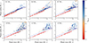 |
Fig. 1. MR diagram for different stellar masses. The colour bar represents the total water mass fraction in the planets. Dots correspond to the nominal output, diamonds to collisions. The brown- and blue-dashed lines correspond to a theoretical composition of Earth-like and 50% water + 50% Earth-like, as defined in Appendix B.5, with dark-blue indicating condensed-water worlds and light-blue indicating steam worlds. The green-dotted curves correspond to 50% steam + 50% Earth-like from Aguichine et al. (2021) (Teq = 400 K for dark-green and Teq = 600 K for light-green). Grey dots are real exoplanets with mass and radius measurements better than 75 and 20%, respectively (data taken from the NASA Exoplanet Archive on 08.09.23). The real exoplanets in each panel correspond to the stellar masses of 0–0.25 M⊙ for M⋆ = 0.1 M⊙, 0.25–0.55 M⊙ for M⋆ = 0.4 M⊙, 0.55–0.85 M⊙ for M⋆ = 0.7 M⊙, 0.85–1.15 M⊙ for M⋆ = 1.0 M⊙, 1.15–1.4 M⊙ for M⋆ = 1.3 M⊙, and 1.4–1.7 M⊙ for M⋆ = 1.5 M⊙. |
A general trend that we find for all panels, is a division given by the rocky and condensed-water lines. Bare rocky cores cluster around the Earth-like composition (as they should based on our assumptions) and wet planets tend to be either on the condensed-water line or above. This diagonal band between the rocky and condensed-water lines remains planet-depleted for all stellar masses (although some planets with intermediate compositions exist in between those lines, particularly for M dwarfs; see Fig. 1). Planets with radii larger than the one given by the condensed-water line tend to have substantial H/He, particularly when moving towards larger planet mass. This can be appreciated as a fading of the blue colour towards large planetary radii (the mass fraction of water decreases as the H/He mass fraction increases). The H/He mass fraction of each synthetic planet is also depicted in Fig. B.4. Another clear trend of Fig. 1 is that for M⋆ ≥ 0.7 M⊙, a large number of water-worlds cluster around the steam line (particularly for M⋆ = 0.7 M⊙). Indeed, for those cases the temperatures are high enough for water to be present in the form of steam throughout the atmosphere. This is demonstrated in Appendix B.4. Other aspect analysed in detail in Appendix B.7 is the presence of “red” outliers among “blue” planets. These are planets that actually formed beyond the ice line but lost most of their water during evolution.
We also note from Fig. 1 that the lower the stellar mass, the larger the overlap in mass and radius of dry and wet planets. As the stellar mass increases, the minimum mass of wet planets increases as well, taking values of Mmin≃ 0.6, 1.4, 2.8, 4.5, 5.4 and 7.3 M⊕ for M⋆ = 0.1, 0.4, 0.7, 1.0, 1.3, 1.5 M⊙, respectively1. This is the imprint of orbital migration. Indeed, the lower the stellar mass, the lower the threshold mass to undergo type-I migration when embedded in a gaseous disc (Paardekooper et al. 2011). The same effect was reported in Burn et al. (2021). This produces a large overlap in mass and radius between dry and wet planets for M⋆ = 0.1 M⊙, filling the radius valley, as noted in the histograms of Fig. B.2 for M⋆ ≲ 0.4 M⊙. The radius valley starts to clearly emerge for M⋆ ≳ 0.7 M⊙, where water worlds have typical masses above 2–3 M⊕.
3.2. Valley in the radius-stellar mass plane
Different analysis of exoplanet data have shown that the radius valley follows a power-law dependence with stellar mass, namely,
 (1)
(1)
For KGF stars from the Kepler data, Berger et al. (2020) found  , and Petigura et al. (2022),
  ,
,  . For M dwarfs, Luque & Pallé (2022) found m = 0.08 ± 0.12.
In Fig. 2, we plot the planet radius as a function of the stellar mass for our synthetic planets, colour-coded by fH2O, as in Fig. 1. The blue-dotted line represents our best fit of the valley adopting the power-law dependence of Eq. (1). The location of the valley was found using the open tool https://github.com/parkus/gapfit (Loyd et al. 2020).
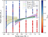 |
Fig. 2. Radius valley fit as a function of the stellar mass (blue line with errors in light-blue) for all our synthetic planets (colour-coded as a function of the water mass fraction). Dots correspond to the nominal output, diamonds to collisions. The green dashed line with the light-green shaded area show the best fit found by Petigura et al. (2022), the violet dashed line and the lilac shaded area represent the results found by Berger et al. (2020), and the mustard dashed line and the light-mustard shaded area represents the best fit by Luque & Pallé (2022). Our best fit was found using https://github.com/parkus/gapfit (Loyd et al. 2020). |
By adopting RV0, guess = 1.82 and mguess = 0.09 in gapfit, our best fit yields Rv, 0 = 1.8197 and  . We note that we are not plotting the 1σ error computed with gapfit, but the best fit with the corresponding errors of the constants Rv, 0 and m. We also over-plot the fits from previous studies with their corresponding errors in Fig. 2 (see figure caption). Our theoretical results are in excellent agreement with the observational results, for all the stellar masses ranging from 0.1 to 1.5 M⊙. Figure 2 also shows that for M⋆ ≲ 0.4 M⊙, the radius valley fades (or, in other words, it gets filled), because of the increasing overlap between rocky and water worlds (see Fig. 1). A vanishing radius valley for M dwarfs is observationally supported by the findings of Luque & Pallé (2022) and Ho et al. (2024). Another remarkable aspect of Fig. 2 is that for M⋆ ≳ 0.7 M⊙, the radius valley is actually empty, particularly for M⋆ ≥ 1.3 M⊙. This is in agreement with the findings of Van Eylen et al. (2021) and Ho & Van Eylen (2023).
3.3. Valley in the radius-orbital period plane
We additionally analysed the location of the valley as a function of orbital period using gapfit for KGF stars and M dwarfs. The result of the best fit for KGF-stars is  and is shown in Fig. 3, together with the fit derived by Petigura et al. (2022),
  . We note that including A type stars (M⋆ = 1.5 M⊙) does not alter the fit. Despite the limitations of our model (too many planets concentrated at Porb ≈ 11 − 15 days, see Sect. 2 and Appendix A.6), we find a remarkable good agreement with observations, with a negative slope carved by photoevaporation. For M dwarfs (M⋆ = 0.1 and 0.4 M⊙), we find a slope of
  , i.e. a flat slope, in line with Luque & Pallé (2022) – who found a slope of −0.02 ± 0.05 –, and also in agreement (within errors) with Bonfanti et al. (2024), who derived a slope of
  . However, we caution that in this case the package gapfit cannot easily find a gap, with different initial guesses yielding different slopes. This is not a problem related to a lack of points (with other pairs of stellar bins this problem does not arise), which reinforces the conclusion that the valley gets indeed filled when moving towards M dwarfs.
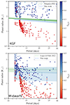 |
Fig. 3. Radius valley fit as a function of orbital period (blue line with errors in light-blue). The colour bar indicates total water mass fraction. Top panel: Planets around KGF-type stars. The green line and shade show the best fit found by Petigura et al. (2022) for these stellar types. Bottom panel: Planets around M dwarfs. The green line and shade show the best fit found by Luque & Pallé (2022). The particular clustering in the orbital period in both panels is due to the model limitations (Appendix A.6). |
4. Discussion: Compositional valley
We computed the growth and post-formation evolution of planets orbiting starts from 0.1 to 1.5 M⊙. Several model limitations exist, which we discuss in detail in Appendix A.6. Overall, our findings reinforce our conclusion of V20 that the radius valley is a separator in planetary composition between bare rocky cores whose atmospheres were stripped off by photoevaporation and water worlds that formed beyond the ice line and retained some or none of their primordial H/He. However, the radius valley fades with decreasing stellar mass (Figs.1–3). This is a consequence of orbital migration, which happens for less massive planets at lower stellar masses (Paardekooper et al. 2011; Burn et al. 2021). Hence, for low mass-stars, originally small icy planets that formed beyond the ice line can reach the inner regions of the system, rendering a larger overlap in mass and radius between planets formed inside and outside the ice line for M dwarfs.
Nevertheless, the paucity of planets with intermediate values of water mass fraction (0 < fH2O ≲ 0.2) persists for all stellar masses, yielding a depleted (M⋆ ≤ 0.4 M⊙) or empty (M⋆ ≥ 0.7 M⊙) diagonal band in the MR diagram of Fig. 1 between the rocky and condensed-water lines. This is due to pebble accretion, which proceeds quickly beyond the ice line, typically allowing the planets to reach the pebble isolation mass before crossing it. This means that solid accretion tends to stops before the icy planets have the possibility to accrete dry pebbles and mix their bulk composition (particularly true for M⋆ ≳ 1.0 M⊙). If this “diagonal valley” were to not be confirmed by future observations, then planetesimal-based (e.g. Brügger et al. 2020) or hybrid pebble-planetesimal models (Alibert et al. 2018; Guilera et al. 2020) would be favoured. Alternatively, it could indicate a slower pebble accretion resulting from a lower fragmentation velocities of icy pebbles. This “diagonal valley” in the M-R diagram appears more clearly when plotting, instead of radius, mean density (normalised by the density of an Earth-like composition, as in Luque & Pallé 2022, also see Appendix B.6). We show this in Fig. 4, including the compositional lines of Earth-like, pure-silicate composition, condensed-water, and steam worlds. The colour bars indicate the planetary equilibrium temperature and the different symbols give the different stellar masses (0.1–0.7 M⊙ on the left panel, 1.0–1.5 M⊙ on the right). A clear pattern emerging from Fig. 4 is a depletion (void) of planets with ρ ≈ 0.6 − 0.9 ρ⊕, S around stars of 0.1–0.7 M⊙ (1.0–1.5 M⊙). Our model assumes an Earth-like composition for all the rocky components. In reality, different stellar abundances would yield rocky planets with different iron fractions, implying that rocky planets could be expected down to the pure silicate line (in orange) of Fig. 4. This means that, in reality, the density valley would be more blurred, but should still exist at ρ ≈ 0.6 − 0.8 ρ⊕, S as a consequence of pebble accretion. This is overall in line with the conclusions of Luque & Pallé (2022), who found a valley at ρ ≈ 0.65 ρ⊕, S for M-planets.
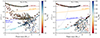 |
Fig. 4. Density-mass diagram (density normalised by an Earth-like composition) as a function of equilibrium temperature (colour bar). Left panel: Planets orbiting stars of 0.1 M⊙ (circles), 0.4 M⊙ (squares), and 0.7 M⊙ (diamonds). Right panel: Planets orbiting stars of 1.0 M⊙ (circles), 1.3 M⊙ (squares), and 1.5 M⊙ (diamonds). Note: the colour bars span different ranges in the two panels. For both panels, black-bordered symbols indicate fHHe < 1%, dark-grey 1 ≤ fHHe ≤ 10%, and light-grey fHHe > 10%. The dashed-lines show the compositional curves of Earth-like (brown), pure-silicate (orange), condensed water (blue), and steam worlds (light-blue). The grey-dotted lines correspond to radii of 1 and 4 R⊕. |
We note as well that water worlds with “condensed” water exist mainly for M⋆ = 0.1 and 0.4 M⊙, where the equilibrium temperatures are below ∼400 K (Fig. 4, bottom left, and Fig. C.2). For 0.7 M⊙, water-worlds are very common, but water is present as steam along all the planetary envelope. Thus, for planets with Teq ≳ 400 K, we predict that water worlds should cluster around the line of 50% rock and 50% steam by mass (at approx. 0.2–0.4 ρ⊕, S), as long as planetary cores are built predominately from pebbles. This steam line has planetary radii larger than the condensed-water line by 30–50% for planetary masses of 1 − 5 M⊕, following the tendency reported by Turbet et al. (2019) and Aguichine et al. (2021). This means that the existence of steam-worlds helps to carve a deeper radius valley for Teq ≳ 400 K (also reported by Burn et al. 2024, for planets around Sun-like stars, with Teq ≳ 600 K). In this regard, our results do not entirely match those of Luque & Pallé (2022), who report water worlds of Teq > 400 K falling on the condensed-water line. A possible explanation might be steam atmospheres with a reduced water mass fraction (see discussion in Appendix C.3). Increasing the sample of M planets will be crucial for testing our model predictions.
Finally, Figs. 1 and 4 also illustrate how mini-Neptunes range from being predominantly water-condensed worlds for M⋆ = 0.1 and 0.4 M⊙, to steam worlds for M⋆ = 0.7 M⊙, to steam-H/He planets for M⋆ ≳ 1.0 M⊙, with a H/He mass fraction below 10%. This prediction holds within the ranges in equilibrium temperature considered in this work (see Fig. 4). The case of M⋆ = 1.5 M⊙ appears somehow to be the exception, where several mini-Neptunes are dry due to the high loss of water during evolution (see Fig. 1 and Appendix B.7).
5. Conclusions
We studied the combined formation and evolution of planets around single stars in the mass range 0.1 ≤ M⋆ ≤ 1.5 M⊙, with the goal of characterising the radius valley for different stellar types. Overall, we find that the tendency (found in V20) of having larger water worlds over smaller rocky planets persists for all stellar ranges, but the radius valley separating them fades towards M dwarfs (in agreement with Luque & Pallé 2022; Bonfanti et al. 2024). This is a consequence of orbital migration, which allows small icy planets to reach the disc inner regions for low-mass stars, producing a larger overlap in mass and radius between the rocky and icy populations.
Despite of the “filling” of the radius valley towards low stellar masses, we find that when considering the full range of stellar masses, its dependence on stellar mass is in excellent agreement with observations, following  . We also find a good agreement with observations regarding the location of the radius valley with orbital period (see Sect. 3.3), with a negative slope carved by photoevaporation for KGF-stars and a flat slope for M dwarfs.
Our end-to-end simulations show that super-Earths are bare rocky cores that emerge as evaporated worlds around all stars. On the other hand, mini-Neptunes, are, in their vast majority, water worlds that lost all or part of their primordial H/He due to photoevaporation. In addition, we confirm that the particular phase of water is key in shaping the radii of the exoplanet population. If the outer atmospheric temperatures are low enough for water to condense (Teq ≲ 400 K), then a water-world will transition from a steam to an icy or liquid world, reducing its size by ∼15% at a planetary mass of 5 M⊕.
Finally, within our pebble-based formation and evolution model, the radius valley emerges as a divider in planetary composition. Thus, we note that it is more visible in terms of mean density, where a clear valley occurs at normalised mean density of ρ/ρ⊕, S ∼ 0.6 − 0.8 across all stellar types.
Mmin is taken as the 5% percentile of the distribution of wet planets, to avoid a few outliers.
Acknowledgments
We thank the anonymous referee for insightful criticism. J.V. acknowledges support from the Swiss National Science Foundation (SNSF) under grant PZ00P2_208945. J.H. and C.M. acknowledge support from the Swiss National Science Foundation (SNSF) under grant 200021_204847 “PlanetsInTime”. M.P.R. is partially supported by PICT-2021-I-INVI-00161 from ANPCyT, Argentina. M.P.R., O.M.G. and M.M.B. are partially supported by PIP-2971 from CONICET (Argentina) and by PICT 2020-03316 from Agencia I+D+i (Argentina). M.P.R. and O.M.G. acknowledge support by ANID, – Millennium Science Initiative Program – NCN19_171. O.M.G. gratefully acknowledges the invitation and financial support from ISSI Bern in early 2024 through the Visiting Scientist Program. Software: For this publication the following software packages have been used: Python-matplotlib (https://matplotlib.org/) by Hunter (2007), Python-seaborn (https://seaborn.pydata.org/) by Waskom et al. (2020), Python-numpy (https://numpy.org/), Python-pandas (https://pandas.pydata.org/).
References
- Aguichine, A., Mousis, O., Deleuil, M., & Marcq, E. 2021, ApJ, 914, 84 [NASA ADS] [CrossRef] [Google Scholar]
- Alibert, Y. 2017, A&A, 606, A69 [NASA ADS] [CrossRef] [EDP Sciences] [Google Scholar]
- Alibert, Y., & Venturini, J. 2019, A&A, 626, A21 [NASA ADS] [CrossRef] [EDP Sciences] [Google Scholar]
- Alibert, Y., Carron, F., Fortier, A., et al. 2013, A&A, 558, A109 [NASA ADS] [CrossRef] [EDP Sciences] [Google Scholar]
- Alibert, Y., Venturini, J., Helled, R., et al. 2018, Nat. Astron., 2, 873 [NASA ADS] [CrossRef] [Google Scholar]
- Andrews, S. M., Wilner, D. J., Hughes, A. M., Qi, C., & Dullemond, C. P. 2010, ApJ, 723, 1241 [Google Scholar]
- Baraffe, I., Homeier, D., Allard, F., & Chabrier, G. 2015, A&A, 577, A42 [NASA ADS] [CrossRef] [EDP Sciences] [Google Scholar]
- Bell, K. R., & Lin, D. N. C. 1994, ApJ, 427, 987 [NASA ADS] [CrossRef] [Google Scholar]
- Benz, W., Broeg, C., Fortier, A., et al. 2021, Exp. Astron., 51, 109 [Google Scholar]
- Berger, T. A., Huber, D., Gaidos, E., van Saders, J. L., & Weiss, L. M. 2020, AJ, 160, 108 [NASA ADS] [CrossRef] [Google Scholar]
- Birnstiel, T., Ormel, C. W., & Dullemond, C. P. 2011, A&A, 525, A11 [NASA ADS] [CrossRef] [EDP Sciences] [Google Scholar]
- Bitsch, B., Morbidelli, A., Johansen, A., et al. 2018, A&A, 612, A30 [NASA ADS] [CrossRef] [EDP Sciences] [Google Scholar]
- Bonfanti, A., Brady, M., Wilson, T. G., et al. 2024, A&A, 682, A66 [NASA ADS] [CrossRef] [EDP Sciences] [Google Scholar]
- Bouchy, F., Wildi, F., & González Hernández, J. I. 2022, European Planetary Science Congress, EPSC2022–937 [Google Scholar]
- Brügger, N., Burn, R., Coleman, G. A. L., Alibert, Y., & Benz, W. 2020, A&A, 640, A21 [NASA ADS] [CrossRef] [EDP Sciences] [Google Scholar]
- Burn, R., Schlecker, M., Mordasini, C., et al. 2021, A&A, 656, A72 [NASA ADS] [CrossRef] [EDP Sciences] [Google Scholar]
- Burn, R., Mordasini, C., Mishra, L., et al. 2024, Nat. Astron., 8, 463 [Google Scholar]
- Cañas, M. H., Lyra, W., Carrera, D., et al. 2024, Planet. Sci. J., 5, 55 [CrossRef] [Google Scholar]
- Chabrier, G., Mazevet, S., & Soubiran, F. 2019, ApJ, 872, 51 [NASA ADS] [CrossRef] [Google Scholar]
- Chen, H. & Rogers, L. A. 2016, ApJ, 831, 180 [NASA ADS] [CrossRef] [Google Scholar]
- Cloutier, R., & Menou, K. 2020, AJ, 159, 211 [NASA ADS] [CrossRef] [Google Scholar]
- Demory, B. O., Pozuelos, F. J., Gómez Maqueo Chew, Y., et al. 2020, A&A, 642, A49 [NASA ADS] [CrossRef] [EDP Sciences] [Google Scholar]
- Drążkowska, J., Alibert, Y., & Moore, B. 2016, A&A, 594, A105 [Google Scholar]
- Drążkowska, J., & Alibert, Y. 2017, A&A, 608, A92 [Google Scholar]
- Drążkowska, J., Stammler, S. M., & Birnstiel, T. 2021, A&A, 647, A15 [Google Scholar]
- Ercolano, B., & Clarke, C. J. 2010, MNRAS, 402, 2735 [Google Scholar]
- Flock, M., Turner, N. J., Mulders, G. D., et al. 2019, A&A, 630, A147 [NASA ADS] [CrossRef] [EDP Sciences] [Google Scholar]
- Freedman, R. S., Lustig-Yaeger, J., Fortney, J. J., et al. 2014, ApJS, 214, 25 [CrossRef] [Google Scholar]
- Fulton, B. J., & Petigura, E. A. 2018, AJ, 156, 264 [Google Scholar]
- Fulton, B. J., Petigura, E. A., Howard, A. W., et al. 2017, AJ, 154, 109 [Google Scholar]
- Ginzburg, S., Schlichting, H. E., & Sari, R. 2018, MNRAS, 476, 759 [Google Scholar]
- Guilera, O. M., & Sándor, Z. 2017, A&A, 604, A10 [Google Scholar]
- Guilera, O. M., Miller Bertolami, M. M., & Ronco, M. P. 2017, MNRAS, 471, L16 [NASA ADS] [CrossRef] [Google Scholar]
- Guilera, O. M., Cuello, N., Montesinos, M., et al. 2019, MNRAS, 486, 5690 [NASA ADS] [CrossRef] [Google Scholar]
- Guilera, O. M., Sándor, Z., Ronco, M. P., Venturini, J., & Miller Bertolami, M. M. 2020, A&A, 642, A140 [NASA ADS] [CrossRef] [EDP Sciences] [Google Scholar]
- Guillot, T. 2010, A&A, 520, A27 [NASA ADS] [CrossRef] [EDP Sciences] [Google Scholar]
- Gundlach, B., & Blum, J. 2015, ApJ, 798, 34 [Google Scholar]
- Gundlach, B., Schmidt, K. P., Kreuzig, C., et al. 2018, MNRAS, 479, 1273 [NASA ADS] [CrossRef] [Google Scholar]
- Gupta, A., & Schlichting, H. E. 2019, MNRAS, 487, 24 [Google Scholar]
- Haldemann, J., Alibert, Y., Mordasini, C., & Benz, W. 2020, A&A, 643, A105 [NASA ADS] [CrossRef] [EDP Sciences] [Google Scholar]
- Haldemann, J., Dorn, C., Venturini, J., Alibert, Y., & Benz, W. 2024, A&A, 681, A96 [NASA ADS] [CrossRef] [EDP Sciences] [Google Scholar]
- Ho, C. S. K., & Van Eylen, V. 2023, MNRAS, 519, 4056 [NASA ADS] [CrossRef] [Google Scholar]
- Ho, C. S. K., Rogers, J. G., Van Eylen, V., Owen, J. E., & Schlichting, H. E. 2024, MNRAS, submitted [arXiv:2401.12378] [Google Scholar]
- Hunter, J. D. 2007, Comput. Sci. Eng., 9, 90 [NASA ADS] [CrossRef] [Google Scholar]
- Ikoma, M., Nakazawa, K., & Emori, H. 2000, ApJ, 537, 1013 [NASA ADS] [CrossRef] [Google Scholar]
- Inamdar, N. K., & Schlichting, H. E. 2015, MNRAS, 448, 1751 [NASA ADS] [CrossRef] [Google Scholar]
- Izidoro, A., Ogihara, M., Raymond, S. N., et al. 2017, MNRAS, 470, 1750 [Google Scholar]
- Izidoro, A., Bitsch, B., Raymond, S. N., et al. 2021, A&A, 650, A152 [EDP Sciences] [Google Scholar]
- Jin, S., & Mordasini, C. 2018, ApJ, 853, 163 [Google Scholar]
- Kegerreis, J. A., Eke, V. R., Massey, R. J., & Teodoro, L. F. A. 2020, ApJ, 897, 161 [NASA ADS] [CrossRef] [Google Scholar]
- Kessler, A., & Alibert, Y. 2023, A&A, 674, A144 [NASA ADS] [CrossRef] [EDP Sciences] [Google Scholar]
- Kippenhahn, R., Weigert, A., & Weiss, A. 2012, Stellar Structure and Evolution (Springer) [Google Scholar]
- Kubyshkina, D. I., & Fossati, L. 2021, Res. Notes Am. Astron. Soc., 5, 74 [Google Scholar]
- Kunimoto, M., & Matthews, J. M. 2020, AJ, 159, 248 [NASA ADS] [CrossRef] [Google Scholar]
- Lambrechts, M., Johansen, A., & Morbidelli, A. 2014, A&A, 572, A35 [NASA ADS] [CrossRef] [EDP Sciences] [Google Scholar]
- Lee, E. J., & Connors, N. J. 2021, ApJ, 908, 32 [NASA ADS] [CrossRef] [Google Scholar]
- Lenz, C. T., Klahr, H., & Birnstiel, T. 2019, ApJ, 874, 36 [NASA ADS] [CrossRef] [Google Scholar]
- Linder, E. F., Mordasini, C., Mollière, P., et al. 2019, A&A, 623, A85 [NASA ADS] [CrossRef] [EDP Sciences] [Google Scholar]
- Lodders, K., Palme, H., & Gail, H. P. 2009, Landolt Börnstein, 44 [Google Scholar]
- Lopez, E. D., & Fortney, J. J. 2013, ApJ, 776, 2 [Google Scholar]
- Loyd, R. O. P., Shkolnik, E. L., Schneider, A. C., et al. 2020, ApJ, 890, 23 [NASA ADS] [CrossRef] [Google Scholar]
- Luque, R., & Pallé, E. 2022, Science, 377, 1211 [NASA ADS] [CrossRef] [Google Scholar]
- Martinez, C. F., Cunha, K., Ghezzi, L., & Smith, V. V. 2019, ApJ, 875, 29 [Google Scholar]
- Matsumoto, Y., Kokubo, E., Gu, P.-G., & Kurosaki, K. 2021, ApJ, 923, 81 [NASA ADS] [CrossRef] [Google Scholar]
- McDonald, G. D., Kreidberg, L., & Lopez, E. 2019, Astrophys. J., 876, 22 [NASA ADS] [CrossRef] [Google Scholar]
- McNally, C. P., Nelson, R. P., Paardekooper, S.-J., & Benítez-Llambay, P. 2019, MNRAS, 484, 728 [Google Scholar]
- Michel, A., Haldemann, J., Mordasini, C., & Alibert, Y. 2020, A&A, 639, A66 [NASA ADS] [CrossRef] [EDP Sciences] [Google Scholar]
- Miguel, Y., Cridland, A., Ormel, C. W., Fortney, J. J., & Ida, S. 2020, MNRAS, 491, 1998 [NASA ADS] [Google Scholar]
- Moldenhauer, T. W., Kuiper, R., Kley, W., & Ormel, C. W. 2022, A&A, 661, A142 [NASA ADS] [CrossRef] [EDP Sciences] [Google Scholar]
- Mordasini, C. 2020, A&A, 638, A52 [NASA ADS] [CrossRef] [EDP Sciences] [Google Scholar]
- Mulders, G. D., Pascucci, I., Apai, D., & Ciesla, F. J. 2018, AJ, 156, 24 [Google Scholar]
- Musiolik, G. 2021, MNRAS, 506, 5153 [CrossRef] [Google Scholar]
- Musiolik, G., & Wurm, G. 2019, ApJ, 873, 58 [NASA ADS] [CrossRef] [Google Scholar]
- Musiolik, G., Teiser, J., Jankowski, T., & Wurm, G. 2016, ApJ, 827, 63 [NASA ADS] [CrossRef] [Google Scholar]
- Nietiadi, M. L., Rosandi, Y., & Urbassek, H. M. 2020, Icarus, 352, 113996 [NASA ADS] [CrossRef] [Google Scholar]
- Ogihara, M., & Hori, Y. 2020, ApJ, 892, 124 [Google Scholar]
- Ogihara, M., Kunitomo, M., & Hori, Y. 2020, ApJ, 899, 91 [NASA ADS] [CrossRef] [Google Scholar]
- Ormel, C. W., Shi, J.-M., & Kuiper, R. 2015, MNRAS, 447, 3512 [Google Scholar]
- Owen, J. E., & Jackson, A. P. 2012, MNRAS, 425, 2931 [Google Scholar]
- Owen, J. E., & Wu, Y. 2017, ApJ, 847, 29 [Google Scholar]
- Paardekooper, S.-J., Baruteau, C., & Kley, W. 2011, MNRAS, 410, 293 [NASA ADS] [CrossRef] [Google Scholar]
- Parmentier, V., & Guillot, T. 2014, A&A, 562, A133 [NASA ADS] [CrossRef] [EDP Sciences] [Google Scholar]
- Parmentier, V., Guillot, T., Fortney, J. J., & Marley, M. S. 2015, A&A, 574, A35 [NASA ADS] [CrossRef] [EDP Sciences] [Google Scholar]
- Petigura, E. A., Rogers, J. G., Isaacson, H., et al. 2022, AJ, 163, 179 [NASA ADS] [CrossRef] [Google Scholar]
- Psaridi, A., Bouchy, F., Lendl, M., et al. 2022, A&A, 664, A94 [NASA ADS] [CrossRef] [EDP Sciences] [Google Scholar]
- Raymond, S. N., Boulet, T., Izidoro, A., Esteves, L., & Bitsch, B. 2018, MNRAS, 479, L81 [Google Scholar]
- Ricker, G. R., Winn, J. N., Vanderspek, R., et al. 2015, J. Astron. Telesc. Instrum. Syst., 1, 014003 [Google Scholar]
- Rogers, J. G., Gupta, A., Owen, J. E., & Schlichting, H. E. 2021, MNRAS, 508, 5886 [NASA ADS] [CrossRef] [Google Scholar]
- Ronco, M. P., Guilera, O. M., & de Elía, G. C. 2017, MNRAS, 471, 2753 [NASA ADS] [CrossRef] [Google Scholar]
- Rosotti, G. P. 2023, New Astron. Rev., 96, 101674 [NASA ADS] [CrossRef] [Google Scholar]
- Savvidou, S., & Bitsch, B. 2023, A&A, 679, A42 [NASA ADS] [CrossRef] [EDP Sciences] [Google Scholar]
- Schneider, A. D., & Bitsch, B. 2021, A&A, 654, A71 [Google Scholar]
- Seager, S., Kuchner, M., Hier-Majumder, C. A., & Militzer, B. 2007, ApJ, 669, 1279 [NASA ADS] [CrossRef] [Google Scholar]
- Selsis, F., Leconte, J., Turbet, M., Chaverot, G., & Bolmont, É. 2023, Nature, 620, 287 [NASA ADS] [CrossRef] [Google Scholar]
- Tanigawa, T., & Ikoma, M. 2007, ApJ, 667, 557 [NASA ADS] [CrossRef] [Google Scholar]
- Turbet, M., Ehrenreich, D., Lovis, C., Bolmont, E., & Fauchez, T. 2019, A&A, 628, A12 [NASA ADS] [CrossRef] [EDP Sciences] [Google Scholar]
- Van Eylen, V., Agentoft, C., Lundkvist, M. S., et al. 2018, MNRAS, 479, 4786 [Google Scholar]
- Van Eylen, V., Astudillo-Defru, N., Bonfils, X., et al. 2021, MNRAS, 507, 2154 [NASA ADS] [Google Scholar]
- Venturini, J., Guilera, O. M., Haldemann, J., Ronco, M. P., & Mordasini, C. 2020a, A&A, 643, L1 [NASA ADS] [CrossRef] [EDP Sciences] [Google Scholar]
- Venturini, J., Guilera, O. M., Ronco, M. P., & Mordasini, C. 2020b, A&A, 644, A174 [NASA ADS] [CrossRef] [EDP Sciences] [Google Scholar]
- Wang, Y., Ormel, C. W., Huang, P., & Kuiper, R. 2023, MNRAS, 523, 6186 [NASA ADS] [CrossRef] [Google Scholar]
- Waskom, M., Gelbart, M., & Botvinnik, O., et al. 2020, https://doi.org/10.5281/zenodo.592845 [Google Scholar]
- Zeng, L., Jacobsen, S. B., Sasselov, D. D., et al. 2019, Proc. Natl. Acad. Sci., 116, 9723 [Google Scholar]
Appendix A: Methodology
A.1. Formation model: Initial conditions
We applied the global planet formation model PLANETALP (Ronco et al. 2017; Guilera & Sándor 2017; Guilera et al. 2019) with stellar masses of 0.1, 0.4, 0.7, 1.0, 1.3, and 1.5 M⊙. As in V20, we used the 12 protoplanetary disc profiles from Andrews et al. (2010), with two uniform viscosity parameters (α = 10−4, 10−3), where the initial gas surface density is given by:
 (A.1)
(A.1)
where Σg, 0 is a normalisation parameter determined by the disc initial mass (Md, 0), γ is the exponent that represents the surface density gradient, and rc is the characteristic or cut-off radius of the disc. Following Burn et al. (2021), we scale the initial disc mass and characteristic radii as:
 (A.2)
(A.2)
 (A.3)
(A.3)
where  and
and  stem from Andrews et al. (2010) (displayed in Tab. B.1 of Venturini et al. 2020a). In Venturini et al. (2020a), we considered only solar-mass stars and we set the inner edge of the disc at 0.1 au, based on hydrodinamical simulations (Flock et al. 2019) and on the mean orbital period of the innermost planet of planetary systems (Mulders et al. 2018). Also, as in Burn et al. (2021), we scale the disc inner edge as:
 (A.4)
(A.4)
This scaling is based on identifying the location of rint as the point where the Keplerian orbital period matches the stellar rotation period (assumed to be the same for all stars as in Burn et al. 2021). However, we note that the location of the disc inner edge and its scaling with stellar mass is very uncertain.
Given the initial gas surface density by Eq. (A.1), the initial dust surface density is defined as
 (A.5)
(A.5)
where ηice represents the sublimation/condensation of water-ice and adopts values of ηice = 1/2 inside the ice line and ηice = 1 outside of it (Lodders et al. 2009). Z0 is the initial dust-to-gas ratio (adopting values of 0.0068, 0.0099, 0.0144, 0.0210, and 0.0305) to span the known ranges of stellar metallicities (as assumed in V20). Regarding the thermodynamical quantities of the discs around stars with different masses, we used the corresponding effective temperatures, Teff, and stellar radii, R⋆, from Baraffe et al. (2015) for the different protostars at 0.5 My to compute the disc vertical structure (as in Guilera et al. 2017, 2019).
As in Venturini et al. (2020a), we launch seven embryos per disc (one at a time), three of them are inside and four of them beyond the ice line. For the embryos that start within the ice line in the solar-case, the initial semi-major axis is defined with uniform log-spacing between rint and rice − 0.1 au, and between rice + 0.1 au and 16 au for the icy embryos. For the non-solar cases, the corresponding initial semimajor axis scales as aini(M⋆/M⊙)1/3 as the disc’s inner edge.
A.2. Gas accretion: Calculation and assumptions
Gas accretion is computed both in the attached and detached phases as in Venturini et al. (2020b). During the attached phase (where the planet’s envelope connects smoothly with the gaseous disc), gas accretion is calculated by solving the 1D spherically symmetric structure equations for the envelope before the planet reaches the pebble isolation mass (following the method of Alibert & Venturini (2019), which uses deep neural networks trained on pre-computed structure models for sub-critical core masses). When solving the structure equations, the envelope opacity is taken from Freedman et al. (2014) for the gas, and from Bell & Lin (1994) for the dust (see the discussion on the choice of opacities in Appendix C.1.3.) Once the pebble isolation mass is attained, solid accretion stalls and the core becomes critical. At this stage, we adopt the prescription of Ikoma et al. (2000), which is valid precisely in this regime when solid accretion is halted. After reaching the pebble isolation mass, at a certain point, the planet would accrete more gas than what the disc can provide due to its viscosity. Here, the planet detaches from the disc and accretes at a rate given by the disc viscous accretion (3πνΣ). In the detached phase, the gas accretion can be damped even further when the planet opens a gap. This is taken into account following Eqs. (36)-(39) of Tanigawa & Ikoma (2007).
A.3. Gas removal by giant impacts
Once the gas of the disc has completely dispersed, during the first million years of evolution, giant collisions between the remaining planets and embryos may become an important mechanism for efficiently removing the planet’s atmosphere (Ogihara & Hori 2020; Ogihara et al. 2020) before atmospheric mass loss due to photoevaporation takes place (Izidoro et al. 2017). Here, as in Venturini et al. (2020a), we formed seven embryos per disc, but only one at a time, which implies that N-body interactions between protoplanets embedded in the gaseous disc are not modelled. However, we can simply estimate the atmospheric mass-loss due to potential collisions between the formed planet and another one less massive with final period < 100 days, also formed in the same disc, but in a different simulation. For the sake of simplicity and in alignment with the findings of Ogihara & Hori (2020), who observed one or two giant impacts in their N-body analysis, we restricted each planet to a single collision. We follow the procedure developed in Ronco et al. (2017), where the core mass of the planet after the collision is the sum of the target’s and impactor’s cores, and where the final envelope mass (ME) is estimated with the global atmospheric mass-loss fractions (Xloss) computed in Inamdar & Schlichting (2015) (their Fig.5) between super-Earths and mini-Neptunes. Thus, if  and
and  are the envelope masses of the target, i, and the impactor, j, the envelope mass of the target after the collision is given by
  , where
  and
and  are the atmospheric mass-loss fractions of the target and the impactor, respectively. For each family of collisions (i.e. for all the isolated collisions between a planet and each of the other less massive planets in the same disc), we kept the most destructive one, which removes the greatest amount of atmosphere.
The main caveat of our simple collision model is clearly the lack of N-body simulations since we can only handle one planet per simulation. Our approach to calculating potential collisions post-gas stage with other (less massive) planets formed under the same initial disc conditions in different simulations does not guarantee their simultaneous formation in a single simulation. On the other hand, considering only one collision per planet, particularly the most destructive one (the one that generates the maximum envelope mass-loss), could reduce the mass of the envelope between 16%-100%, with a mean value of 72%, as stated in Appendix D of V20. This consideration could be overestimating the envelope mass-loss rate since Ogihara & Hori (2020) showed that their mass-loss fraction ranges from a few percent to approximately 90%, but with a typical value around 20%. However, they also confirm that this percentage is higher if head-on collisions take place. On another note, Matsumoto et al. (2021), who conducted N-body simulations to trace planet sizes during the giant impact phase with envelope stripping through impact shocks, considering empirical envelope-loss rates obtained from smoothed particle hydrodynamics simulations by Kegerreis et al. (2020). These authors also mentioned that head-on collisions can lead to increased rates of envelope mass loss. Additionally, their findings indicate that protoplanets in inner orbits undergo a higher frequency of collisions, potentially leading them to become bare cores after giant impacts. This is an outcome we also found within our simulations. Thus, our model captures the overall outcomes observed in more detailed studies, despite its simplicity and reduced precision in modelling collisions.
A.4. Evolution model
After disc dispersal and the removal of mass from giant impact (for the ’collision case’), we computed the cooling and contraction of the planets’ envelopes, including the effect of mass-loss due to photoevaporation during 2 Gyr with the code COMPLETO (Mordasini 2020). We refer to this stage as the ’evolution’ phase. The choice of 2 Gyr is to ensure that all the stars considered in this study are still in the main sequence. The code solves the 1D equations for mass, momentum, and energy conservation. When calculating the luminosity evolution, the gravitational and internal energy of the core and envelope, as well as radiogenic heating were considered (Linder et al. 2019). The stellar X-ray flux evolution was taken from the model of McDonald et al. (2019). The envelopes are assumed to be composed of H, He, and H2O (with the compounds uniformly mixed) and with the initial amounts stemming from the accretion process. The equation of state (EOS) of the H/He component corresponds to Chabrier et al. (2019) and for water, we use the AQUA EOS from Haldemann et al. (2020). The EOS for the iron-silicate core is the modified polytropic EOS of (Seager et al. 2007), which does not yield very precise planetary radii for sub-Earth size planets. For this reason, we re-computed the final radius at 2 Gyr with the more-up-to-date interior structure model of BICEPS (see next section). The atmospheric escape rates are taken from (Kubyshkina & Fossati 2021). The atmospheric escape follows a dependency of  (Owen & Jackson 2012; Mordasini 2020), where Zenv is the water mass fraction of the envelope, namely,
  . We caution that the evaporation rates of envelopes enriched in heavy elements are still uncertain. It is imperative that future hydrodynamic escape calculations address this aspect.
A.5. Transit radius calculation and internal structure
At the end of the planetary evolution stage, for each modelled planet, we calculated its corresponding transit radius. For that purpose, we used the internal structure model of BICEPS by Haldemann et al. (2024). BICEPS solves the internal structure equations and calculates the planetary transit radius for a large range of planetary compositions. For this work, we assumed that all planets are structured in the following way: i) in the centre there is an iron core made out of pure iron, ii) surrounded by a mantle of rocky material (MgSiO3), and iii) the outermost layer contains the volatile elements H, He, and H2O. The composition of the volatile layer is given by MHHe and MH2O, which are provided for each planet by the evolution model. As in V20, the water is uniformly mixed with the H, and He; thus, Zenv is uniform throughout the volatile layer. For planets that lost all their volatiles during the evolutionary stage or did not accrete any volatiles, the structure model starts the integration at the mantle layer. We note that the mass ratio between iron core and rocky mantle is kept at Earth-like values of 1:2.
Depending on the planet’s internal luminosity, the orbital distance to its host star and the host stars effective temperature the thermal structure of the volatile layer will be different. To account for this effect, BICEPS uses the non-grey atmosphere model of Parmentier et al. (2015) to calculate the temperature profile of the outermost volatile layer. We further use the Schwarzschild criterion to determine if at a certain depth the volatile layer is stable against convection, namely, if the temperature gradient is radiative or adiabatic (Kippenhahn et al. 2012). At last the transit radius is calculated by determining the radius at the chord optical depth of τchord = 2/3 (Guillot 2010; Parmentier & Guillot 2014). The opacities used in this calculation are taken from Freedman et al. (2014). For more details on the internal structure model (especially the applied EOSs), we refer to Haldemann et al. (2024).
A.6. Model limitations
Several simplifications affect the results of our formation-evolution-structure calculations.
-
Solar elemental abundances:
-
(a)
The rocky component of the planets is always assumed to be Earth-like in composition, namely, with 33% iron and 67% silicates by mass. In reality, a spread in iron and silicate abundances is expected for stars that have elemental abundances different than solar. The minimum iron mass fraction expected for stars in the thin disc (where the Sun and most planet-hosting stars are) is of ∼20%, (Michel et al. 2020, their Fig. A.1).
-
(b)
The ice-to-rock ratio of 1:1 just beyond the ice line also stems from solar abundances. Stars with other elemental abundances are expected to exhibit different ratios. For thin-disc stars, the minimum water mass fraction of solid material beyond the ice line is of ∼30% (Michel et al. 2020, see their Fig. A.2).
These two compositional assumptions imply that the "depleted diagonal band" found in the MR diagram of Fig.1 should still exist, but could be narrower, between lines of 20% iron mass fraction for rocky composition and of 30% water mass fraction. This would also translate in a persistent density valley for all stellar types between the same compositional lines.
-
(a)
-
Only one planetary seed per disc: N-body interactions are not yet included in PLANETALP. This implies that the planet typically reaches the disc inner edge when migrating inwards, and the possibility of being trapped in resonant chains with other planets at different semi-major axes cannot be modelled. This model limitation has a stark impact on the planets’ final orbital period, which should not be directly compared to observations.
-
Planetary seeds are all placed at the beginning of the simulations (time = 0). This also affects the final orbital period of wet versus rocky planets. Formation timescales are shorter for wet planets (as we showed in V20) and, as a consequence, they reach the inner disc at early times, when the zero torque location (the planet migration trap) is located near the inner edge of the disc. As time evolves, this migration trap location moves slightly outwards and dry planets tend to be trapped at larger periods. This is why in Fig. 3, we can see that most of the wet planets tend to be located at orbital periods of ∼12 days, while the dry ones are mostly located at orbital periods of ≳13 days.
-
Planetary cores are assumed to grow only due to pebbles. In reality, pebbles are converting into planetesimals in the disc (Drążkowska & Alibert 2017; Lenz et al. 2019), thus planetesimals could also contribute to the core growth. Except for very few cases (Alibert et al. 2018; Guilera et al. 2020; Kessler & Alibert 2023), formation models tend to assume only one of the two solid accretion types due to the uncertain pebble-to-planetesimal ratios along the disc. Planetesimal accretion would yield more mixed compositions (Brügger et al. 2020; Burn et al. 2021), blurring the density valley to some extent.
-
The atmospheric escape rates for atmospheres enriched in water are taken from empirical photoevaporation laws from protoplanetary discs (Ercolano & Clarke 2010) (Sect.A.4). Detailed hydrodynamical atmospheric escape simulations for mixtures of H, He and H2O should be developed in the future.
-
Simplifications in the internal structure calculations: our upper irradiated atmospheres assume a solar composition (Parmentier et al. 2015). In addition, the gas opacities in the radiative zones are calculated with the model of Freedman et al. (2014), which accounts for certain degree of envelope enrichment, but are not specific to water.
Appendix B: Extended results
B.1. Bare cores after disc dissipation
The effect found in V20 is in principle expected to occur for any stellar mass because it is related to the change of the pebbles’ properties at the water ice line. This, in turns, produces more massive icy cores than rocky ones and this effects the core sizes as well.
In Fig. B.1, we show the histograms of the core sizes of the simulated planets at the end of formation. The blue bars indicate a core water mass fraction larger than fH2O, core > 45%, the red ones, dry cores (fH2O, core < 5%), and the green bars intermediate, mixed compositions (5%≤fH2O, core ≤ 45%). We note that, as expected, icy cores tend to be bigger than rocky cores, for all stellar masses. A deficit of cores with sizes in the range of ∼1.5 − 2 R⊕ is clear for M⋆ ≥ 0.4 M⊙. The valley separates dry from wet cores for M⋆ ≥ 0.4 M⊙. Interestingly, the lower the stellar mass, the larger the overlap in size between the dry and wet populations, and the larger the number of planets with intermediate compositions. In particular, for M⋆ = 0.1 M⊙ there is no second peak, as many icy cores are very small. This behaviour is due to migration. Type I migration occurs for lower planet mass at lower stellar masses (Paardekooper et al. 2011). This allows for smaller icy planets to reach the inner system for the low stellar mass cases. This feature was also reported by Burn et al. (2021).
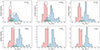 |
Fig. B.1. Histograms of core sizes at the end of formation, for the different stellar masses, and for planets with final orbital period below 100 days. Red bars indicate fH2O, core < 5%, green bars 5%≤fH2O, core < 45%, and blue bars fH2O, core ≥ 45%, where fH2O, core is the core water mass fraction at the end of formation. The black lines show the overall core size distribution. |
B.2. After 2 Gyr of evolution
Figure B.2 shows the histograms of the planet radii at 2 Gyr of evolution, for both the nominal and collisional cases. In agreement with Fig. B.1, the radius valley is non-existent for M⋆ = 0.1 M⊙, and starts to be visible for M⋆ ≥ 0.4 M⊙ for the collisional case (which resembles, rather, the bare core cases of Fig. B.1 since more atmospheric mass is removed when we allow for giant impacts). Interestingly, our model predicts that the case of M⋆ = 0.7 M⊙ is the one for which the radius valley is the most prominent, with a clear peak of water-rich mini-Neptunes for both nominal and collisional cases. This is in line with the findings of Kunimoto & Matthews (2020) which report the occurrence rate of mini-Neptunes increasing for K dwarfs compared to G dwarfs. It is important to clarify that these histograms should not be taken as absolute occurrence rates to compare directly with observations. Indeed, this study is not a population synthesis, in the sense that the initial conditions are not taken with the weights of the observed distributions of disc properties. We do consider the ranges of possible initial conditions stemming from observations, but not the weights of the distributions. Nevertheless, the fractions of certain types of planets (e.g. mini-Neptunes) can be compared relatively, between our different stellar masses. Our planet formation and evolution parameter study predicts that mini-Neptunes reach their peak of occurrence for stellar masses of M⋆ ∼ 0.7 M⊙ (strictly speaking, 0.4 < M⋆ < 1.0 M⊙ due to our binning in stellar mass). For the nominal cases of M⋆ ≳ 1.0 M⊙, the water-rich planets are no longer concentrated around a peak value, but they are, rather, spread over a large range of sizes. This is mainly the effect of gas accretion onto cores that are more massive compared to M⋆ ≲ 1.0 M⊙ and which can bind larger amounts of gas. When gas is removed by collisions, the mini-Neptune peak re-emerges, similarly to what we found in V20. Another effect that removes mini-Neptunes for the case of the most massive stars (M⋆ ≳ 1.3 M⊙) is the strong photoevaporation, which completely removes the H/He/H2O envelopes for more planets compared to M⋆ = 1.0 M⊙. Hence, planets that were born beyond the ice line as ice-rich, can become bare rocky cores by evolution. In our simulations, this happens for 28% of the original water-rich mini-Neptunes for M⋆ = 1.5 M⊙ and for 14% of the original water-rich mini-Neptunes for M⋆ = 1.3 M⊙.
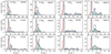 |
Fig. B.2. Histograms of planets’ radii after 2 Gyr of evolution, for different stellar masses, and for planets with final orbital period below 100 days. Red bars indicate |


B.3. Water-worlds around low-mass stars migrated from beyond the ice line
The ice line of protoplanetary discs around low-mass stars is much closer to the central star than for more massive stars. For example, while for M⋆ = 1.0 M⊙, the ice line typically locates initially at ∼2-3 au, for M⋆ = 0.1 M⊙ it is at∼0.5 au at the beginning of the simulations. Because of this, the existence of water worlds around low-mass stars could in principle be explained without type I migration, in a scenario where wet-planets with orbital periods below 100 days simply formed in situ, with the ice line closer in. However, this never happens in our simulations, water worlds always accrete the bulk of their ices beyond the ice line and migrate inwards afterwards. To illustrate this, we show in the top panel of Fig. B.3 that the ice lines in discs around M⋆ = 0.1 M⊙ never manage to cross the 100-day orbit threshold (marked with the horizontal grey dashed line at ∼0.2 au) before photoevaporation opens a gap in the disc (time from which the solid lines become dashed lines). The bottom panel of Fig. B.3 shows that planets forming within the ice line for M⋆ = 0.1 M⊙ are always dry (planetary tracks represented with black curves only), while those that start their growth outside the ice line, but end inside it are water-rich (planetary tracks represented by turquoise curves that then turn into black once they cross the ice line) and can only reach the regions of orbital period below 100 days (marked by the dashed vertical line) through type I migration. We have checked that this scenario always takes place with all the icy planets around all the stars considered. For simplicity we only show it for some of them, selected randomly, around 0.1 M⊙.
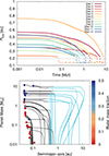 |
Fig. B.3. Time evolution of the ice lines for the discs around 0.1M⊙ (top) for the different protoplanetary discs considered in our simulations (see Sect.A.1, for α = 10−4). The ice lines turn from solid to dashed lines when the mid-gap opens in the protoplanetary disc (i.e. when the disc dissipates at the ice line’s location). The horizontal grey dashed line represents the orbit of ∼100 days. Growth tracks of planets forming around 0.1M⊙ that end within the 100-day period (bottom). Black lines indicate that the planet is located inside the ice line, while torquoise lines indicate the planet is beyond the iceline. Clearly, all planets that had accreted some ice started to form beyond a 100-day period. |
B.4. Steam atmospheres
An interesting feature of Fig.1 is that for M⋆ ≥ 0.7 M⊙, most of the water-rich, H/He-poor planets (fH2O > 0.45 and fHHe < 10−2, see Figs.1 and B.4) lie above the condensed-water line. To understand what is is behind the ’puffing up’ of the water-rich planets, we first need to isolate the effect of H/He from the effect of temperature on the planetary radii. For this, we plot in Fig.B.5 the M-R diagram as a function of equilibrium temperature for M⋆ = 0.4.−0.7 M⊙. The planets are also distinguished by a H/He mass fraction smaller or larger than 0.01 (we refer to them as H/He poor if fHHe < 10−2 and H/He-rich otherwise). Three things are clear from this diagram:
-
Water-rich and H/He-poor planets with the lowest equilibrium temperature (below 400 K, the ones around M⋆ = 0.4 M⊙) lie on the condensed-water line. These planets are cold enough for water to be in condensed form.
-
All of the water-rich, H/He-poor planets with Teq ≥ 400 K lie on a different line (light blue in the figure). They are well described as RP(MP) =
 , with a = 1.64183 and b = 0.180572 (see Sect.B.5).
 -
All the planets with fHHe ≳ 10−2 are scattered either above the light-blue M-R curve for M⋆ = 0.7 M⊙ or above the condensed-water line for M⋆ = 0.4 M⊙.
 |
Fig. B.5. MR diagram of water-rich planets (fH2O ≥ 0.45) around M⋆ = 0.4 M⊙ (circles) and M⋆ = 0.7 M⊙ (diamonds). Black-bordered symbols indicate fHHe ≤ 10−2, while grey, fHHe > 10−2. The colour bar is the equilibrium temperature of the planets at zero albedo. The dashed-blue line shows the condensed-water line, the light-blue dashed a fitting MR relation to the steam worlds, described in Sect.B.5. |
Indeed, for all the planets with fHHe > 10−2, the radius is strongly affected by the amount of primordial gas and by the equilibrium temperature. On the other hand, the planets that follow the light-blue line are H/He poor but their full atmospheres are hot enough for water to be present as vapour. This is better illustrated in Fig.C.2 where we show specific pressure-temperature atmospheric profiles (Appendix C.2).
B.5. MR relations: Analytical fits
In this section, we specify the mass-radius (MR) analytical curves deployed in Fig.1. Such MR relations were obtained by fitting our results for the rocky, condensed-water, and steam planets computed with BICEPS (Sect.A.5.)
For rocky planets, defined as those planets with final water contents lower than 5% in mass and H-He envelopes lower than 10−6 with respect to the total mass, we find the following relation:
 (B.1)
(B.1)
with arocky = 0.999009 ± 0.0002802 and brocky = 0.279514 ± 0.0002377. Our fit is in very good agreement with the one found by Zeng et al. (2019), who found arocky = 1 and brocky = 1/3.7 ≈ 0.27027. We note that we do not have any bare rocky planet with mass larger than 10 M⊕, reason for which this fit is valid for planetary masses below that.
For condensed-water planets, which are planets with a final water content greater than 45% in terms of mass (and less or equal than 50% due to the assumed ice-to-rock ratio at the ice line), H-He envelopes lower than 10−2 by mass, and Teq < 400 K, we find:
 (B.2)
(B.2)
with acw = 1.24191 ± 0.001667, and bcw = 0.267404 ± 0.0008558. The fit was performed for planets with 0.1 ≤ MP ≤ 20 M⊕ and therefore should only be used in this mass range. We note again that our fit is in very good agreement with the one found by Zeng et al. (2019) for those planets with 50% of water by mass, who found acw = 1.24, and bcw = 1/3.7 ≈ 0.27027.
Finally, for the steam-worlds, defined as the condensed-water worlds except that Teq ≥ 400 K, we obtain the following fit:
 (B.3)
(B.3)
with asteam = 1.64183 ± 0.008192, and bsteam = 0.180572 ± 0.001608. The fit was performed for planets with 1 ≤ MP ≤ 40 M⊕ and should only be used in this mass range. We note that our calculations indicate an increase of planet radius of 30%, 25%, and 10% between steam worlds and condensed-water worlds of masses of 1, 2, and 5 M⊕, respectively (for planets with water mass fractions of 50%). As an interesting final remark, we note that the MR relation we find for steam worlds does not depend strongly on equilibrium temperature for different stellar masses.
B.6. Mean density: Histograms
Figure B.6 shows the histograms of the planetary mean densities for the different stellar masses. The left panels are for the planets around the M and K dwarfs, while the right panel for planets orbiting G-F and A stars. In the top panels, the density refers to the ‘normalised density’, namely, the mean density divided by the density that the planet would have if it had an Earth-like composition (i.e. a mass radius-relation given by Eq. B.1). The bottom panels display the histograms of the physical density in cgs. Clearly, the density valley is better visualised in terms of the normalised density, especially for the low-mass stars. The peak of planets at 0.5-0.6 ρ/ρ⊕, S of the left-top panel corresponds to the condensed-water worlds, which do not exist in our results for high-mass stars due to the higher equilibrium temperatures (see Fig. 4). In terms of physical density (bottom panels), the valley occurs at ρ≈ 4-5 g/cm3 for M and K dwarfs, and for ρ≈ 3-4 g/cm3 for G-F-A spectral types.
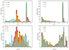 |
Fig. B.6. Planetary mean density for the different stellar masses. Left (right) panels show values for the low- (high-)mass stars, with the each colour corresponding to one stellar mass as indicated in the legend. The top panels show the normalised density (see text), while the bottom panels show the density in cgs. |
B.7. A few dry mini-Neptunes in the MR diagram
Figure 1 contains a few dry ‘outliers’ in the region of the MR diagram above the condensed-water line, where most planets are water-rich. These planets were actually formed beyond the ice line, just like the wet planets that surround them. The difference with the latter is that they lost most of their water (and H/He) due to photoevaporation during the evolutionary phase. To illustrate this, we show in Table B.1, the initial and final planet mass, water mass, and H/He mass for two planets that end up very close in the MR diagram of M⋆ = 1.5 M⊙. We also tabulate the rock mass (invariable during the evolution), and the initial and final water mass fraction (fH2O), H/He mass fraction (fHHe) and envelope metallicity (Zenv, defined as the mass of water divided by the mass of water plus H/He). One of the planets ends up water-rich and
Physical quantities of two planets around M⋆ = 1.5 M⊙ that finish with very similar mass and radius but with very different compositions. "Initial" and "final" refer to the onset and end of the evolutionary phase, respectively. The mass of rocks remains invariant during the evolution.
the other water-poor after 2 Gyr of evolution (referred as ‘wet’ and ‘dry’ planets in the table, respectively). The reason behind the different evolutionary paths is the atmospheric escape rate going as  (with Zenv being the envelope water mass fraction, which remains constant throughout the evolution by hypothesis). This means that the smaller the initial Zenv, the faster the atmospheric mass loss. Indeed, the two planets have very different initial Zenv, despite of having similar initial fH2O. The smaller Zenv of the dry planet is a consequence of having a much larger initial amount of H/He. Because of the smaller Zenv of the dry planet, it loses 99.45% of its initial envelope during 2 Gyr of evolution, while the ‘wet’ planet loses only 6.46% of it. This leaves the ‘dry’ planet with only fH2O = 0.55% for the bulk water fraction at the end of the evolutionary phase, while the ‘wet’ planet retains fH2O = 47.6%. Despite being highly ‘desiccated’, the dry planet would still show a high water signature in its atmospheric spectra, due to it retaining an atmospheric water mass fraction (or envelope metallicity) of Zenv ≈ 55%. We caution, however, that atmospheric escape rates of envelopes enriched with elements heavier that H/He are highly uncertain and that more theoretical research is needed to provide meaningful predictions of water mass fraction during the evolutionary phase.
Appendix C: Extended discussions
C.1. Dependence of the radius valley location on the formation model parameters
Planet formation models contain a set of free parameters, with a range of possible values inferred from either observations or lab experiments. These parameters can affect the outcome of planet formation simulations in regard to the predicted planet mass, planet radius, and orbital distance to the star, among others. The prime parameters that can result in very different outcomes in our pebble-based formation model are:
-
the α-viscosity parameter
-
the fragmentation threshold velocity of pebbles
-
the opacity of the gaseous envelope
While a deep analysis of the impact of these parameters on our results is beyond the scope of the present work, it is nevertheless pertinent to discuss the effect they could have on the location of the radius valley.
C.1.1. Dependence on the α-viscosity parameter
The α-viscosity parameter affects the growth of the planetary cores in two ways. On the one hand, it affects the pebbles’ sizes (the higher the α, the more turbulent is the disc, hence the more the pebbles collide and break, maintaining the pebbles at smaller sizes). The larger the pebbles, the faster the core grows (e.g. Lambrechts et al. 2014; Venturini et al. 2020b). On the other hand, the disc viscosity impacts the disc’s structure, including the disc aspect ratio. This means that the pebble isolation mass (the maximum mass a core can acquire by pebble accretion) is indirectly affected by α, because the pebble isolation mass depends strongly on the disc aspect ratio. In principle, the larger the α, the larger the pebble isolation mass, because the larger the viscosity, the more massive the planet needs to be to open a partial gap. We checked that the pebble isolation mass at the ice line is of about 8 M⊕ for α = 10−5, compared to ∼15 M⊕ for α = 10−4 for a standard disc around a Sun-like star. A planet of 8 M⊕ with fH2O = 0.5 and without H-He would have a size of 2.86 R⊕ (from using the MR relation of Eq.B.3), which means that the mean of water-worlds forming at such low viscosity are still expected to contribute mainly to the peak of mini-Neptunes and not to fill the radius valley (at ≈1.8 − 1.9 R⊕ for M⋆ = 1.0 M⊙).
In Venturini et al. (2020b), we discussed extensively the impact of α on the planetary growth by pebble accretion within the ice line, considering values of α = 10−5, 10−4and10−3 (which are the values inferred from disc observations; see e.g. Rosotti 2023). We found that for α = 10−3, the rocky pebbles were so small (∼10 μm) that planets were basically not growing inside the ice line. On the other extreme, for α = 10−5, we found that the pebbles reach much bigger sizes (∼1 cm) in the dry inner regions, and planetary growth proceeds extremely fast (in the order of 104 years). We also found that for the formation of rocky cores, considering α = 10−5 increases the maximum bare rocky core mass from 5 M⊕ to 7 M⊕ with respect to α = 10−4. This would still yield a maximum radius of bare rocky cores of 1.69-1.95 R⊕ (from using the MR relation of (Zeng et al. 2019) and of Eq.B.1), that is, at the location of the valley.
It is also important to mention that the planet migration prescriptions adopted in our model are not really valid for α ∼ 10−5. For such small values of α, even a low-mass planet could open a partial gap. McNally et al. (2019) showed that in this case, vortices form at the edges of the partial gap, changing the migration regime. Thus, based on our previous results, in this work we decided to keep the same approach as in V20, using only α = 10−4 and α = 10−3. We analysed the effect of this two values of the α-viscosity parameter on the location of the radius valley on Fig.C.1. The plot shows the MR diagrams for the synthetic planets, distinguishing according to the cases where α = 10−4 (orange circles) or α = 10−3 (green triangles). Overall, we notice that the void of the ‘diagonal band’ delimited by the Earth-like composition and the condensed-water lines (which sets the location of the radius and density valley; see main text) is preserved for both values of α. For α = 10−3, we have very few rocky planets, which is expected due to the extremely low pebble sizes, resulting in negligible core growth inside the ice line (Venturini et al. 2020b). Overall, the jump in pebble size at the ice line is the underlying reason for the dichotomy in core size and core composition in our pebble-based formation model (Venturini et al. 2020a). This jump exists at any value of the α-viscosity parameter (Fig. 4, top panel, from Venturini et al. 2020b).
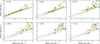 |
Fig. C.1. MR diagrams according to the adopted values of the α-viscosity parameter. Green triangles: α = 10−3. Orange circles:α = 10−4. Both nominal and collisional cases are displayed. |
C.1.2. Dependence on the fragmentation threshold velocity of pebbles
Regarding the impact of the fragmentation threshold velocities on the results, in V20 we showed that for Sun-like stars, considering vth= 1 m/s for silicates and vth= 5 m/s for icy pebbles gives very similar results to our nominal assumption of vth= 1 m/s for silicates and vth= 10 m/s for icy pebbles. If instead vth = 2 m/s is chosen for the icy pebbles, fewer planets with the maximum core ice mass fraction of 0.5 form and more planets with intermediate ice compositions emerge. This would contribute to the filling of the radius valley. Finally, we tested as well a very low fragmentation threshold velocity of vth= 1 m/s, constant along the disc. In that case, the pebbles remain so small along the disc, that planet formation by pebble accretion is very inefficient: no planet forms with mass above Earth and no planet migrates within 100 days of orbital period.
The values of the fragmentation threshold velocity suited for protoplanetary disc conditions have been a topic of intense debate in the past years. The values adopted in this work (10 m/s beyond the water-ice line and 1m/s within the ice line), are the standard values used in dust growth and evolution studies (Drążkowska et al. 2016; Drążkowska & Alibert 2017), and on planet formation models, (e.g. Drążkowska et al. 2021; Schneider & Bitsch 2021; Savvidou & Bitsch 2023). These values are also supported by many experimental works (e.g. Gundlach & Blum 2015; Musiolik et al. 2016). While recent laboratory experiments found that amorphous water-ice particles could be as fragile as silicates (e.g. Gundlach et al. 2018; Musiolik & Wurm 2019), more recent works, such as those of Nietiadi et al. (2020) and Musiolik (2021), revealed that ices of various volatile molecules on the surface of dust aggregates act like liquids during collisions. This behaviour increases the sticking properties and enables higher velocity collisions that do not lead to the fragmentation of ice-coated dust aggregates. Thus, given the current knowledge on the topic, we consider that a value of 10 m/s for the fragmentation threshold velocity of ice-rich grains is a sufficiently reasonable assumption. In addition, fragmentation threshold velocities of 1 m/s for silicate and 10 m/s for icy pebbles were recently adopted by Cañas et al. (2024) to explain the density dichotomy in the Kuiper Belt Objects. For our results, the location of the radius valley is invariant as long as the fragmentation threshold velocity of icy pebbles is in the range of 5-10 m/s.
C.1.3. Dependence on the envelope’s opacity
The opacities in the gaseous envelope control its cooling and contraction and, hence, the gas accretion rate as long as the planet’s envelope connects smoothly with the gaseous disc (attached phase). The largest uncertainty in the opacity values stem from the poorly constrained grain sizes within a planetary envelope. In principle, grains can settle and grow compared to ISM sizes, which goes in the direction of reducing the dust opacities compared to the ISM. However, the level of turbulence in planetary envelopes is hard to predict, the growth of grains depends upon their size and structure (e.g. fractal versus non-fractal, which is unknown), as well on the magnitude of the envelope ‘recycling’. Indeed, recent 3D hydrodynamical simulations have shown that as long as a planet is located at short orbital distances (within approximately 1 au from the central star Ormel et al. 2015; Moldenhauer et al. 2022; Wang et al. 2023), the gas that is accreted by the planet can flow back to the protoplanetary disc. This means that for planets building the envelopes at short orbital distances (as in our scenario, where planets migrate fast towards the disc inner edge and continue accreting gas at the stranded locations), the small dust grains would be constantly replenishing the envelopes as fresh gas flows in. This is why we chose the high grain opacity values from Bell & Lin (1994), which correspond to the ISM size grains (and whose values vary with pressure and temperature).
In any case, due to the uncertainty on the dust opacity values of the planetary envelopes during planet formation, it is worth discussing its impact on the location of the radius valley. The study of Mordasini (2020) studies the emergence of the radius valley taking initial conditions from population synthesis studies that assume (contrary to our assumptions) a very low dust opacity during the formation phase (Bell & Lin 1994, reduced by a factor of 0.003). The location of the valley, corresponding to the maximum mass of bare rocky cores, is at 1.67 R⊕ at 0.1 au for a Sun-like star Mordasini (2020, as seen in his Fig.4). We obtained the exact same value in our simulations with high dust opacity (nominal case of M⋆ = 1.0 M⊙ displayed in Fig.B.2). Indeed, Mordasini (2020) discussed the practically negligible effect of the opacities on the radius valley location in Sect.2.3.7 of that paper. This is because at the end of disc lifetime, the lower the envelope dust opacity, the more massive the gaseous envelope for a given core mass. A more massive envelope is more extended than a thin one, which increases the atmospheric escape rate (which depends on the planet radius to the cube Owen & Wu 2017; Mordasini 2020). Thus, even if the planet started with a thicker envelope, photoevaporation would remove it completely for the ranges of core masses we are discussing here (below approximately 10 M⊕). We found this exact same behaviour in our study of Venturini et al. (2020b) when we tested a set of simulations with 100× reduced Bell & Lin (1994) opacities, namely: the location of the radius valley was unchanged.
C.2. Condensed-water or steam worlds: Dependence on equilibrium temperature and model assumptions
It is well known that the atmospheric composition, the distribution of heavy elements and the choice of irradiation model affect the calculation of the planetary radii (Guillot 2010). In V20, we argued that assuming the water as mixed with H/He was the most physically motivated assumption since for Sun-like stars all our synthetic planets had temperatures high enough for water to be in the form of steam throughout all the atmospheres. In this work, we made the same assumption of water mixed with H/He during the evolution simulations and the computation of the planetary radii. However, we noted that our synthetic planets can now have temperatures low enough for water to condense, particularly around M dwarfs (our M⋆ = 0.1, 0.4 M⊙ cases, Appendix B.4). The fate of condensed water in H2O-H-He atmosphere is not trivial to predict. In principle, condensed water on the top layers would settle into deeper regions and if there is atmospheric circulation, would rise up again. Thus, the assumption of uniform envelope metallicity might still hold. For the case of pure water envelopes, a better physical treatment would be to allow water to sink to the next layer, as long as the condensation conditions in pressure and temperature hold. Unfortunately, our structure code cannot handle yet compositional gradients properly. However, we caution that changing the distribution of water will probably change the value of planet radius in cases where water condensation takes place. Not only does the distribution of water affect the resulting transiting radius, but also other model assumptions, such as the choice of opacities and the irradiation model. We note that, compared to our results, the models of Aguichine et al. (2021) predicted a substantially larger planet radius for planets composed of half-rocks-half-water by mass when Teq ≥ 400K (their Fig. 5). The key difference with our model is their assumption of the core-envelope boundary to be extremely hot (in a region of the phase diagram of water where water is in ’supercritical’ state). This assumption is based on evolution calculations accounting for the ‘runaway greenhouse effect of water’ (e.g. Turbet et al. 2019). More recent work points out that such effect might have been overestimated in the past due to the assumption of purely convective envelopes (Selsis et al. 2023).
In our calculations, we did not impose any condition on the pressure-temperature of the envelope-core boundary, we simply integrated the structure equations inwards from the top of the atmosphere (with the outer boundary conditions depending on the equilibrium temperature and on the luminosity that the planet irradiates according to its cooling history; see Appendix A.4). The types of P-T profiles that we find for planets with pure water envelopes are illustrated in Fig.C.2. In the figure, we show the profiles of two planets, one of the two has a fully condensed water envelope while the other a full steam one. To better capture the transition between the two, we ran the case of the steam world again, but reducing its equilibrium temperature (red and green curves of Fig.C.2). We note that the transition between the condensed and steam worlds happens for 383 < Teq < 396K; in our model, this translates into a temperature at the top of the atmosphere of 268 < Tout < 276 K, respectively. The reason for Tout being smaller that Teq by ∼80 − 120 K is the non-grey atmospheric model of Parmentier et al. (2015). The previous grey atmospheric model of Guillot (2010) also yields Tout smaller than Teq, but only by ∼20 K. The nearly 100 K difference in Tout between the two atmospheric models makes the water of the planets orbiting M⋆ = 0.4 M⊙ take a condensed form when using the non-grey irradiated model of Parmentier et al. (2015) (used in COMPLETO) – as compared to the vapour form when using the one of Guillot (2010) (used in COMPLETO). This is shown in Fig. C.3. To summarise, the radii of water-worlds near the condensation line are very sensitive to model assumptions. More efforts are needed in modelling the atmospheres of water worlds to compute accurate transit radii.
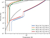 |
Fig. C.2. Pressure-temperature profiles of two synthetic mini-Neptunes with fH2O = 0.5 and equilibrium temperatures of 466 K (planet 503, blue line) and 326 K (planet 506, orange line). The black solid lines in the background are the phase boundaries of pure H2O given by the AQUA EOS (Haldemann et al. 2020). Both planets have a similar mass of approx. 1.5 M⊕, but different sizes due to the different physical state of water (planet 503 is a steam-world, with RP = 1.690 R⊕ , and planet 506 is a condensed-water world with RP = 1.657 R⊕ ). The red and green curves correspond to planet 503, but the equilibrium temperature was reduced to see where the transition from steam to condensed-water world occurs. |
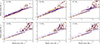 |
Fig. C.3. MR diagrams comparing planetary radii obtained with BICEPS (purple triangles) versus COMPLETO (orange circles). For both set-ups water is assumed to be mixed uniformly with the H/He. |
C.3. Locating the steam worlds
A controversial aspect of the Luque & Pallé (2022) study is the conclusion that the planets that fall on the condensed-water line in the MR diagram are indeed 50% rock+50% condensed water by mass, because most of those exoplanets are too hot for water to be condensed. Our models suggest that an upper equilibrium temperature for the transition would be 400 K, and other works point to even lower temperatures (e.g. Aguichine et al. 2021). The bulk of planets in the sample from Luque & Pallé (2022) have equilibrium temperatures higher than this. To analyse this in more detail, comparing the results of our calculations with observations, we plot on the top panels of Fig. C.4, all real exoplanets with Teq ≤ 400 K for 0.25 ≤ M⋆ < 0.55 M⊙ (M dwarfs) and Teq ≤ 600 K for 0.55 ≤ M⋆ < 0.85 M⊙ (K dwarfs).
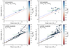 |
Fig. C.4. Comparison of real exoplanets for M⋆ = 0.4 M⊙ (left panels) and M⋆ = 0.7 M⊙ (right panels). The limit in equilibrium temperature is for proper comparison with our simulations. The brown- and blue-dashed lines correspond to Earth-like and 50% water+50% Earth-like compositions, with dark-blue indicating condensed-water and light-blue, steam-worlds (as defined in Appendix B.5). The green-dotted curves correspond to 50% steam+50% Earth-like from Aguichine et al. (2021) (Teq = 400 K for dark-green and Teq = 600 K for light-green). The real exoplanets are those with a relative error in radius less than 25% and in mass of less than 70%, with the data taken form the NASA Exoplanet Archive on 08.09.23. For the bottom panels, the real exoplanets are shown in the background in grey. |
For the M dwarfs, we note that only six real exoplanets have Teq ≤ 400 K and fairly good mass and radius measurements. Three of those have mass and radius compatible with the condensed-water line (within errors). We note that for the planets that have sizes above the condensed-water line, we actually have synthetic planets with that mass and radius (Fig.C.4, bottom-left panel). These planets, despite of having water in condensed form, have some remnant H/He that increases the planet radii compared to the condensed-water line.
For the K dwarfs (Fig.C.4, right panels), the coldest real planet (Teq ≈ 350 K) falls exactly on the condensed-water line, as our calculations predict. Another five real planets fall in between the steam- and condensed-water lines, where our model predicts that the atmospheres should be in the form of steam. Nevertheless, we do have synthetic planets in that region of the parameter space (bottom-right panel). These planets have actually steam atmospheres but the total water content is of fH2O ≈ 20 − 40% (Fig.1). Thus, this could be a plausible explanation for the real exoplanets falling in between the steam- and condensed-water lines for Teq ≳ 400 K (composition that could also explain the exoplanets analysed by Luque & Pallé 2022).
We also note that while our model yields some steam-worlds with masses between 1 and 3 M⊕ and Teq ≈ 500 − 600 K for M⋆ = 0.7 M⊙, no real exoplanets have yet been confirmed in that part of the parameter space (see top-right panel of Fig. C.4). Nevertheless, the synthetic planets falling in that part of the MR diagram represent only 5% of the synthetic water worlds produced for that stellar mass, so we expect those planets to be rare. In addition, we note that the number of sub-Neptunes around K dwarfs with Teq ≤ 600 K is still low to draw any strong conclusions.
Another clear difference between the synthetic and real exoplanets observed in this figure is the lack of real rocky exoplanets. This is because of the imposed maximum equilibrium temperature. Real rocky exoplanets exist but typically at higher equilibrium temperatures. Improved modelling on the disc inner edge and the addition of N-body interactions and orbital evolution due to tides is needed to better reproduce the observed distribution of planetary periods.
All Tables
Physical quantities of two planets around M⋆ = 1.5 M⊙ that finish with very similar mass and radius but with very different compositions. "Initial" and "final" refer to the onset and end of the evolutionary phase, respectively. The mass of rocks remains invariant during the evolution.
All Figures
|
Fig. 1. MR diagram for different stellar masses. The colour bar represents the total water mass fraction in the planets. Dots correspond to the nominal output, diamonds to collisions. The brown- and blue-dashed lines correspond to a theoretical composition of Earth-like and 50% water + 50% Earth-like, as defined in Appendix B.5, with dark-blue indicating condensed-water worlds and light-blue indicating steam worlds. The green-dotted curves correspond to 50% steam + 50% Earth-like from Aguichine et al. (2021) (Teq = 400 K for dark-green and Teq = 600 K for light-green). Grey dots are real exoplanets with mass and radius measurements better than 75 and 20%, respectively (data taken from the NASA Exoplanet Archive on 08.09.23). The real exoplanets in each panel correspond to the stellar masses of 0–0.25 M⊙ for M⋆ = 0.1 M⊙, 0.25–0.55 M⊙ for M⋆ = 0.4 M⊙, 0.55–0.85 M⊙ for M⋆ = 0.7 M⊙, 0.85–1.15 M⊙ for M⋆ = 1.0 M⊙, 1.15–1.4 M⊙ for M⋆ = 1.3 M⊙, and 1.4–1.7 M⊙ for M⋆ = 1.5 M⊙. |
| In the text | |
|
Fig. 2. Radius valley fit as a function of the stellar mass (blue line with errors in light-blue) for all our synthetic planets (colour-coded as a function of the water mass fraction). Dots correspond to the nominal output, diamonds to collisions. The green dashed line with the light-green shaded area show the best fit found by Petigura et al. (2022), the violet dashed line and the lilac shaded area represent the results found by Berger et al. (2020), and the mustard dashed line and the light-mustard shaded area represents the best fit by Luque & Pallé (2022). Our best fit was found using https://github.com/parkus/gapfit (Loyd et al. 2020). |
| In the text | |
|
Fig. 3. Radius valley fit as a function of orbital period (blue line with errors in light-blue). The colour bar indicates total water mass fraction. Top panel: Planets around KGF-type stars. The green line and shade show the best fit found by Petigura et al. (2022) for these stellar types. Bottom panel: Planets around M dwarfs. The green line and shade show the best fit found by Luque & Pallé (2022). The particular clustering in the orbital period in both panels is due to the model limitations (Appendix A.6). |
| In the text | |
|
Fig. 4. Density-mass diagram (density normalised by an Earth-like composition) as a function of equilibrium temperature (colour bar). Left panel: Planets orbiting stars of 0.1 M⊙ (circles), 0.4 M⊙ (squares), and 0.7 M⊙ (diamonds). Right panel: Planets orbiting stars of 1.0 M⊙ (circles), 1.3 M⊙ (squares), and 1.5 M⊙ (diamonds). Note: the colour bars span different ranges in the two panels. For both panels, black-bordered symbols indicate fHHe < 1%, dark-grey 1 ≤ fHHe ≤ 10%, and light-grey fHHe > 10%. The dashed-lines show the compositional curves of Earth-like (brown), pure-silicate (orange), condensed water (blue), and steam worlds (light-blue). The grey-dotted lines correspond to radii of 1 and 4 R⊕. |
| In the text | |
|
Fig. B.1. Histograms of core sizes at the end of formation, for the different stellar masses, and for planets with final orbital period below 100 days. Red bars indicate fH2O, core < 5%, green bars 5%≤fH2O, core < 45%, and blue bars fH2O, core ≥ 45%, where fH2O, core is the core water mass fraction at the end of formation. The black lines show the overall core size distribution. |
| In the text | |
|
Fig. B.2. Histograms of planets’ radii after 2 Gyr of evolution, for different stellar masses, and for planets with final orbital period below 100 days. Red bars indicate |
| In the text | |
|
Fig. B.3. Time evolution of the ice lines for the discs around 0.1M⊙ (top) for the different protoplanetary discs considered in our simulations (see Sect.A.1, for α = 10−4). The ice lines turn from solid to dashed lines when the mid-gap opens in the protoplanetary disc (i.e. when the disc dissipates at the ice line’s location). The horizontal grey dashed line represents the orbit of ∼100 days. Growth tracks of planets forming around 0.1M⊙ that end within the 100-day period (bottom). Black lines indicate that the planet is located inside the ice line, while torquoise lines indicate the planet is beyond the iceline. Clearly, all planets that had accreted some ice started to form beyond a 100-day period. |
| In the text | |
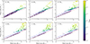 |
Fig. B.4. Same as Fig.1 but the colour bar represents the planets’ mass fraction of H/He. |
| In the text | |
|
Fig. B.5. MR diagram of water-rich planets (fH2O ≥ 0.45) around M⋆ = 0.4 M⊙ (circles) and M⋆ = 0.7 M⊙ (diamonds). Black-bordered symbols indicate fHHe ≤ 10−2, while grey, fHHe > 10−2. The colour bar is the equilibrium temperature of the planets at zero albedo. The dashed-blue line shows the condensed-water line, the light-blue dashed a fitting MR relation to the steam worlds, described in Sect.B.5. |
| In the text | |
|
Fig. B.6. Planetary mean density for the different stellar masses. Left (right) panels show values for the low- (high-)mass stars, with the each colour corresponding to one stellar mass as indicated in the legend. The top panels show the normalised density (see text), while the bottom panels show the density in cgs. |
| In the text | |
|
Fig. C.1. MR diagrams according to the adopted values of the α-viscosity parameter. Green triangles: α = 10−3. Orange circles:α = 10−4. Both nominal and collisional cases are displayed. |
| In the text | |
|
Fig. C.2. Pressure-temperature profiles of two synthetic mini-Neptunes with fH2O = 0.5 and equilibrium temperatures of 466 K (planet 503, blue line) and 326 K (planet 506, orange line). The black solid lines in the background are the phase boundaries of pure H2O given by the AQUA EOS (Haldemann et al. 2020). Both planets have a similar mass of approx. 1.5 M⊕, but different sizes due to the different physical state of water (planet 503 is a steam-world, with RP = 1.690 R⊕ , and planet 506 is a condensed-water world with RP = 1.657 R⊕ ). The red and green curves correspond to planet 503, but the equilibrium temperature was reduced to see where the transition from steam to condensed-water world occurs. |
| In the text | |
|
Fig. C.3. MR diagrams comparing planetary radii obtained with BICEPS (purple triangles) versus COMPLETO (orange circles). For both set-ups water is assumed to be mixed uniformly with the H/He. |
| In the text | |
|
Fig. C.4. Comparison of real exoplanets for M⋆ = 0.4 M⊙ (left panels) and M⋆ = 0.7 M⊙ (right panels). The limit in equilibrium temperature is for proper comparison with our simulations. The brown- and blue-dashed lines correspond to Earth-like and 50% water+50% Earth-like compositions, with dark-blue indicating condensed-water and light-blue, steam-worlds (as defined in Appendix B.5). The green-dotted curves correspond to 50% steam+50% Earth-like from Aguichine et al. (2021) (Teq = 400 K for dark-green and Teq = 600 K for light-green). The real exoplanets are those with a relative error in radius less than 25% and in mass of less than 70%, with the data taken form the NASA Exoplanet Archive on 08.09.23. For the bottom panels, the real exoplanets are shown in the background in grey. |
| In the text | |
Current usage metrics show cumulative count of Article Views (full-text article views including HTML views, PDF and ePub downloads, according to the available data) and Abstracts Views on Vision4Press platform.
Data correspond to usage on the plateform after 2015. The current usage metrics is available 48-96 hours after online publication and is updated daily on week days.
Initial download of the metrics may take a while.