| Issue |
A&A
Volume 686, June 2024
|
|
|---|---|---|
| Article Number | A304 | |
| Number of page(s) | 12 | |
| Section | Stellar structure and evolution | |
| DOI | https://doi.org/10.1051/0004-6361/202244473 | |
| Published online | 21 June 2024 | |
High-resolution spectroscopy of the intermediate polar EX Hydrae
II. The inner disk radius⋆,⋆⋆
Institut für Astrophysik und Geophysik, Georg-August-Universität, Friedrich-Hund-Platz 1, 37077 Göttingen, Germany
e-mail: k.beuermann@t-online.de
Received:
11
July
2022
Accepted:
25
January
2024
EX Hya is one of the best studied, but still enigmatic intermediate polars. We present phase-resolved blue VLT/UVES high-resolution (λ/Δλ ≃ 16.000) spectra of EX Hya taken in January 2004. Our analysis involves a unique decomposition of the Balmer line profiles into the spin-modulated line wings that represent streaming motions in the magnetosphere and the orbital-phase modulated line core that represents the accretion disk. Spectral analysis and tomography show that the division line between the two is solidly located at ∣υrad ∣ ≃ 1200 km s−1, defining the inner edge of the accretion disk at rin ≃ 7 × 109 cm or ∼10R1 (WD radii). This large central hole allows an unimpeded view of the tall accretion curtain at the lower pole with a shock height up to hsh ∼ 1R1 that is required by X-ray and optical observations. Our results contradict models that advocate a small magnetosphere and a small inner disk hole. Equating rin with the magnetospheric radius in the orbital plane allows us to derive a magnetic moment of the WD of μ1 ≃ 1.3 × 1032 G cm3 and a surface field strength B1 ∼ 0.35 MG. Given a polar field strength Bp ≲ 1.0 MG, optical circular polarization is not expected. With an accretion rate Ṁ = 3.9 × 10⁻¹¹ M⊙ yr−1, the accretion torque is Gacc ≃ 2.2 × 1033 g cm2 s−2. The magnetostatic torque is of similar magnitude, suggesting that EX Hya is not far from being synchronized. We measured the orbital radial-velocity amplitude of the WD, K1 = 58.7 ± 3.9 km s−1, and found a spin-dependent velocity modulation as well. The former is in perfect agreement with the mean velocity amplitude obtained by other researchers, confirming the published component masses M1 ≃ 0.79 M⊙ and M2 ≃ 0.11 M⊙.
Key words: binaries: eclipsing / stars: fundamental parameters / novae, cataclysmic variables / stars: individual: EX hydrae / white dwarfs / X-rays: stars
Reduced spectra are available at the CDS via anonymous ftp to cdsarc.cds.unistra.fr (130.79.128.5) or via https://cdsarc.cds.unistra.fr/viz-bin/cat/J/A+A/686/A304
© The Authors 2024
 Open Access article, published by EDP Sciences, under the terms of the Creative Commons Attribution License (https://creativecommons.org/licenses/by/4.0), which permits unrestricted use, distribution, and reproduction in any medium, provided the original work is properly cited.
This article is published in open access under the Subscribe to Open model. Subscribe to A&A to support open access publication.
1. Introduction
EX Hya is the best studied member of the intermediate polar (IP) subclass of cataclysmic variables (CVs) that has about 150 confirmed members and candidates (see Koji Mukai’s IP catalog1). With an orbital period of 98.26 min, it is one of the few IPs below the period gap. EX Hya has been intensely studied over the last 60 yr, facilitated by its small distance of d = 56.77 ± 0.05 pc (Bailer-Jones et al. 2021) and very low interstellar column density. Nevertheless, the fundamental IP parameters, such as the magnetic moment of the white dwarf (WD), remain uncertain. While there is agreement that EX Hya accretes from a disk via the magnetosphere of the WD, to date it has not been possible to reliably measure the radius rin of the boundary between disk and magnetosphere, a key ingredient for studies of the accretion geometry. The WD in EX Hya is a slow rotator with Pspin = 2π/ω = 67.03 min and the corotation radius rcor approximately equals the Roche radius of the WD, exceeding the circularization radius rcirc by a factor of about three. If EX Hya harbors a standard disk that extends inward to rin < rcirc, the Keplerian speed at the boundary between disk and magnetosphere substantially exceeds the rotation speed υin = ω rin of the field. Accretion then occurs far from spin equilibrium, spinning up the WD on a timescale of 5 × 10⁶ yr (Mauche et al. 2009; Andronov & Breus 2013). The uncertainties with regard to the inner disk radius and the magnetic moment of the WD have led to divergent models of the accretion geometry of EX Hya.
The large-magnetosphere model is based on the suggestion of King & Wynn (1999) that accretion in EX Hya may proceed near spin equilibrium, provided the magnetic field is strong and governs the accretion flow close to L1. A ring is formed in the outer Roche lobe of the WD, from which it accretes over 360° in azimuth, preventing the system from becoming a polar (Norton et al. 2004, 2008). Other authors have discussed their data in the framework of this model (Belle et al. 2002; Mhlahlo et al. 2007). The lack of observable circular polarization (Butters et al. 2009) argues against it.
The extended wings of the Balmer lines in EX Hya were originally assigned to the inner accretion disk of what was then considered a dwarf nova (Breysacher & Vogt 1980; Cowley et al. 1981; Gilliland 1982). This was an obvious choice before the magnetic nature of the WD was finally recognized (Vogt et al. 1980; Kruszewski et al. 1981; Warner & McGraw 1981; Sterken et al. 1983; Cordova et al. 1985). Since the flux in the line wings varies with the spin period, they were subsequently associated with streaming motions in the magnetosphere (Cordova et al. 1985; Hellier et al. 1987; Kaitchuck et al. 1987), although several authors continued to favor a disk origin of part of the line wings (e.g., Belle et al. 2003; Echevarría et al. 2016). The small-magnetosphere model was formally introduced by Revnivtsev et al. (2009), who suggested that an observed break in the power spectra of the X-ray and optical intensity fluctuations of an IP may indicate the orbital frequency at the inner edge of its accretion disk. This model was employed to EX Hya by Revnivtsev et al. (2011), Semena et al. (2014), and Suleimanov et al. (2016, 2019, and references therein) and predicts inner disk radii between rin = 2 and 4R1, with R1 the WD radius. The implication is that Balmer line emission up to velocities between 1800 and 2600 km s−1 originates from the inner disk. Luna et al. (2018) showed this concept to be inconsistent with X-ray results, rendering the size of the inner hole of the disk in EX Hya a controversial issue that is, at the same time, fundamental to the discussion of its accretion geometry.
In this paper, we present a unique decomposition of the emission line profiles into the spin-modulated line wings and the orbital-phase dependent line core. The latter includes emissions from the disk, the S-wave, and the secondary star, and is loosely referred to as the disk component. Its tomography allows a direct measurement of the terminal velocity of the disk component, which translates into the inner radius of the accretion disk. In addition, we find a slight asymmetry or ellipticity of the motion at rin that is also predicted in hydrodynamic model calculations (Bisikalo et al. 2020; King & Wynn 1999).
2. Observations
2.1. Basic information
EX Hya was observed in service mode with the Ultraviolet and Visual Echelle Spectrograph (UVES) at the Kueyen (UT2) unit of the ESO Very Large Telescope (VLT), Paranal/Chile, on January 23 and 26, 2004, continuously for 2.58 and 2.50 h, respectively. A total of 26 and 25 spectra were taken. Exposure times were 300 s with dead times of typically 60 s between exposures, due to readout and overhead. The resulting orbital phase resolution is Δϕ98 ≃ 0.061 and the spin-phase resolution Δϕ67 ≃ 0.090. Spectra in the blue and red arms were obtained simultaneously; the red spectra were extensively discussed by Beuermann & Reinsch (2008, Paper I, hereafter BR08). Table 1 contains a log of the observations. We adopted the ESO UVES pipeline reduction that provides flat fielding, performs a number of standard corrections, extracts the individual echelle orders, and collects them into a combined spectrum. The flux calibration, except for the seeing correction considered below, is also part of the pipeline reduction. The wavelength calibration is derived from spectra taken with a ThAr lamp. The blue spectra cover the wavelength range 3760–4980 Å with a pixel size of 0.030 Å. With a slit width of 1.0″, the full width at half maximum (FWHM) resolution is 0.175 Å and the spectral resolution is λ/Δλ ≃ 27 000 at Hβ. To improve the S/N, we rebinned the data into 0.300 Å bins, giving an effective resolution of λ/Δλ ≃ 16 000 or Δυ = 18.5 km s−1 at Hβ. All times are quoted as UTC and were converted to BJD (TDB) using the tool provided by Eastman et al. (2010)2.
Journal of the VLT/UVES observations of EX Hya in January 2004.
2.2. Wavelength calibration and phase convention
The wavelength calibration of the red spectra was based on telluric molecular lines and was shown to be accurate to 1 km s−1 (BR08). These lines are not present in the blue spectra, which contain, instead, numerous narrow metal emission lines from the illuminated face of the secondary star (BR08, their Sect. 4.2) that allow a check on the wavelength calibration. Trailed spectra of Ca IIλ8498 and Fe Iλ4957 from the observations on 23 and 26 January 2004 are displayed in Fig. 1. We measured the radial velocities of these lines and of Si Iλ3905, by fitting single Gaussians. The velocities are well represented by sinusoids
![$$ \begin{aligned} \upsilon _\mathrm{rad} = K_2^{\prime }\,\mathrm{sin} [2\pi (\phi _\mathrm{HS} +\phi _0)]+\gamma , \end{aligned} $$](/articles/aa/full_html/2024/06/aa44473-22/aa44473-22-eq1.gif)
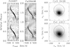 |
Fig. 1. VLT/UVES narrow emission line spectra of Fe Iλ4957 and Ca IIλ8498 observed on 23 and 26 January 2004. Left: grayscale representations of the trailed spectra. Spectral flux increases from white to black. For convenience, the data are shown twice. Right: corresponding tomograms with the Roche lobe contour of the secondary star based on the system parameters of Sect. 3.7 demonstrate the origin from the irradiated face of the secondary star. The relative intensity goes from white (0.0) to black (1.0). The origin of the coordinate system is at the center of gravity. |
where ϕHS refers to the eclipse ephemeris of Hellier & Sproats (1992) against which we measure phase offsets. The fit parameters  , ϕ0, and γ are listed in Table 2. The two rather faint blue lines have γ = −57 ± 3 km s−1 relative to the NIST wavelengths3, which is indistinguishable from the mean γ = −58.2 ± 1.0 km s−1 of the brighter red lines (BR08). We adopt the latter value also for the blue spectra and conclude that the wavelength calibrations in both arms are similarly accurate.
Sine fits to narrow-line radial velocities using the (Hellier & Sproats 1992; HS92) linear orbital ephemeris as reference.
The tomograms of Ca IIλ8498 and Fe Iλ4957 in Fig. 1 demonstrate the sole origin of the lines from the illuminated face of the secondary star. The weighted mean phase offset of the three metal lines is ⟨ϕ0⟩ = 0.0094(16) or O − C = −0.00064(11) days (Table 3). We adopt the blue-to-red zero crossing as inferior conjunction of the secondary star, which occurred at
Observed times of events quoted as BJD (TDB) with errors, and time predicted by either the linear eclipse ephemeris of Hellier & Sproats (1992) or the quadratic ephemeris for the spin maxima of Mauche et al. (2009, their Eq. (1)).
This phasing is used to represent the orbital motion throughout this paper. The light curve of January 26 in Fig. 2 shows the depression caused by the eclipse in time bin 6, coincident with the first spin maximum. With a bin size of 5 min, we can only state that the eclipse occurred within 0.02 in orbital phase from the predicted times on the ephemerides of Hellier & Sproats (1992), Echevarría et al. (2016)4, and Eq. (2).
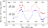 |
Fig. 2. Flux-calibrated spin light curves of the integrated Hβ line flux. The orbital phases are given in the figure. The colored dots indicate the same phase bins as in the left panel. |
The times of four spin maxima of the Hβ flux are listed in Table 3 along with the times predicted by the quadratic ephemeris of Mauche et al. (2009) and the corresponding O − C values. The mean O − C is 0.00094(35) days or −0.020(8) in ϕ67. We adopt spin phases
to match our observations.
2.3. Flux calibration
The observations were performed in good seeing, although somewhat variable, which allowed an absolute calibration of the spectra. To this end, we applied a seeing correction, based on the simultaneous information provided by the Paranal Difference Image Motion Monitor (DIMM, Sarazin & Roddier 1990) and by the width of the individual spectral images perpendicular to the dispersion direction. The two methods yielded similar estimates of the FWHM seeing that varied between 0.9″ and 2.2″ on January 23 and between 0.7″ and 1.2″ on January 26. We corrected each spectrum for the seeing losses assuming a Gaussian point spread function and a source centered in the 1.0″ slit. We estimated the corrected fluxes to have an internal accuracy of better than 20%. Spectral fluxes are quoted in units of 10−16 erg cm−2s−1Å−1.
3. Results
3.1. Analysis of the phase-resolved spectra
Representative information on our spectral data is provided in Figs. 2–4. The left panel of Fig. 4 shows the set of 26 flux-calibrated spectra of 23 January 2004, which cover the Balmer lines Hβ to H11. On each of the two observing nights, 1.5 orbital periods and 2.2 spin periods were covered. Because of the near 3 : 2 commensurability of the two periods, coverage in the ϕ98 − ϕ67 phase space is sparse (left panel in Fig. 3). We decomposed these trailed spectra into the spin modulated line wings and the orbital phase-dependent line core. To this end, we proceeded in a two-step process. In the first step, we constructed a preliminary spin template as the difference between the spectral fluxes at spin maximum and spin minimum, separated by 1.0 orbital and 1.5 spin periods. This choice ensures the best possible subtraction of the S-wave component which approximately repeats on the orbital period. Our data contain three such instances, at ϕ98 = 0.30, 0.65, and 1.00. In the second step, we noted that the line wings of the three preliminary spin templates agree so closely that forming a mean template is warranted. This is then employed to decompose the individual rows of the trailed spectra of both observing nights.
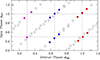 |
Fig. 3. Phase-space coverage of our 51 exposures in the ϕ67–ϕ98 plane. The spectra selected for the spectral decomposition at ϕ98 ≃ 0.30, 0.65, and 1.00 are marked by magenta, blue, and red dots respectively. |
The three orbital phases selected for the first step of the template construction are indicated by the intersections of the dashed lines in the left panel of Fig. 3. To improve the statistics, we formed averages of up to three spectra around the respective phases. These are marked in Fig. 3 by the magenta, blue, and red dots, respectively. The resulting mean spectra at spin maximum and minimum are displayed in the right panel of Fig. 4 as the black and blue curves, respectively. Obtaining the spin templates requires subtraction of the underlying continua from the observed spectra. The high quality of the UVES spectra allows this process to be reliably performed longward of 4100 Å. It is affected in the short-wavelength wing of Hδ by weak disturbing lines and becomes increasingly difficult at shorter wavelengths because of the merging line wings (see Fig. 4, left panel). Consequently, we restricted the analysis to Hβ and Hγ. The fitted continua are depicted as the magenta curves in the right panel of Fig. 4. The spin modulation, which is the difference between the emission line components at spin maximum and minimum, is included in the form of the red curves. Larger representations of the Hβ and Hγ line profiles on a velocity scale are shown in Fig. 5.
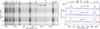 |
Fig. 4. Flux-calibrated blue spectra taken on 23 and 26 January 2004. Left: grayscale representation of the first night, with spectral flux increasing from white to black. Right: mean spectra of the Hγ to Hβ spectral region at spin maximum (black) and spin minimum (blue) for the orbital phases noted in the figure. The best-fit continua that represent the lower envelope to the spectra are shown as magenta curves. The spin modulation of the emission-line component is shown in red. |
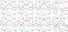 |
Fig. 5. Hβ and Hγ spin maximum and minimum spectra (black and blue, respectively) at ϕ98 = 0.30, 0.65, and 1.0 (six left-most panels). Overplotted are the fitted spin-modulated components fmod(λ) from Eq. (4) with amplitudes Cmax and Cmin (red). Below, the derived disk component is shown (green). The two right panels show the decomposition of the He Iλ4471 line at ϕ98 = 0.0 and 0.30 and of He IIλ4686 at ϕ98 = 0.30. No He II emission from the disk is seen, but S-wave emission is present at other orbital phases (see text). |
3.2. Decomposing the Balmer lines at ϕ98 = 0.3, 0.65, and 1.0
We find that the entire line wings vary to a high degree of accuracy by a spin-phase dependent numerical factor only (i.e., they are multiples of the spin modulation),

which we adopt as a preliminary template at the selected orbital phase (red curves in Fig. 4). We express the line profiles as
and perform the fit only over the line wings. Here δλ allows for a small shift of the template in radial-velocity and δf for an error in subtracting the continuum or a deviation from the assumed proportionality of the line wings to fmod. For vanishing δλ and δf, the wings would vary strictly proportionally to fmod, and the fit parameters Cmax and Cmin would be related by
The validity of our model depends on the degree to which the parameters Cmax and Cmin obtained from the fit comply with Eq. (6). The last term in Eq. (5) designates the core component that is assumed to be the same at spin maximum and minimum and to contribute negligibly in the wings. It is obtained by subtracting the fitted Cfmod and δf from the observed line profile.
The model fits for Hβ and Hγ at the three selected orbital phases are displayed in the six left panels of Fig. 5, now with radial velocity as the abscissa. The black and blue curves are the continuum-subtracted line profiles at spin maximum and minimum. The red curves represent the adjusted spin modulation fitted to both wings over the wavelength ranges indicated by the vertical tick marks. At negative velocities the fits extend to −3000 km s−1 and at positive velocities to about 2100 km s−1, avoiding the disturbing He I lines. The fit excludes the central part of the line, where the fitted fmod deviates drastically from the observed profile. Appropriate limits are ±(1250 ± 50) km s−1 from the line center. The fits are excellent. The fit parameters Cmax and Cmin (noted in the figures) follow Eq. (6) faithfully. The absolute terms δf are close to zero with an average ⟨δf⟩ = 0.5 ± 1.0 in ordinate units. The wavelength shifts δλ stay below ±1.2 Å, equivalent to ∣υrad ∣ < 80 km s−1, consistent with orbital motion and a moderate spin-dependent radial-velocity modulation (see Sect. 3.7). Given that EX Hya is an IP, the highest velocities of the spin component certainly result from the magnetically guided accretion stream near the WD, and since we found that the line wings represent a single entity, this conclusion necessarily holds for the entire spin-modulated component. That the line wings should vary only by a spin-phase dependent factor is not self-evident, but can be understood if spin modulation of the line flux arises mainly from occultation of part of the emission. The core or disk component is clearly limited to radial velocities between ±1300 km s−1. It is displayed at the bottom of the respective figure as the green curve.
The wings of the templates for the three orbital phases agree so closely that it is warranted to combine them into a common final template applicable to all orbital phases. This allows us to decompose the entire body of the trailed spectra and to subject the derived phase-dependent core component to a tomographic analysis. From the tomograms presented in Sect. 3.6, we obtain further insight into the structure of the inner accretion disk.
3.3. Final templates for the Balmer line spin components
We show the normalized mean of the three preliminary templates of Hβ and Hγ in Fig. 6 (blue curves). The central region between ±1200 km s−1 is roughly flat-topped, possibly the result of radiative transfer of the Balmer lines in puffed-up matter of the transition region between the disk and magnetosphere and the bulge of the disk. The remaining fluctuations at the top of the profiles can probably be assigned to imperfect repetition of the S-waves in consecutive orbits. We therefore approximate the central part of the two templates by a flat top (black curves), and adopt these curves as the final spin templates of Hβ and Hγ. In their wings they contain remnants of the nearby He I lines; of additional unidentified faint broad lines of disk origin (Disk); and of narrow metal lines, mostly Fe I, from the secondary star (Fe I). These are all contained in the trailed spectra as well. Only the short-wavelength wing of Hβ is practically free of such disturbances and optimally represents the extended Balmer line wings.
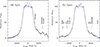 |
Fig. 6. Mean templates of the spin-modulated component of Hβ and Hγ. |
3.4. Decomposing the trailed spectra of Hβ and Hγ
Using the templates of Fig. 6 to represent fmod(λ) in Eq. (5), we decomposed the trailed Hβ and Hγ spectra in the left two panels of Fig. 7. The fits were extended over the same intervals that were used in deriving the templates (tick marks in Fig. 5). The result after subtracting the fitted spin component are labeled in the center panels of Fig. 7 as “Hβ disk” and “Hγ disk”. The dashed lines indicate the ±1200 km s−1 limit, outside of which the disk component rapidly vanishes. The available evidence shows that this limit also holds for the higher Balmer lines (not shown). Since the profile of the template is smooth, all statistical fluctuations of the original spectra are assigned to the disk component. The fitted spin component is featureless and consists of identical rows that vary in intensity with spin phase and display small wavelength shifts. It contains no information of relevance for a tomographic study (Hellier 1999) and is not shown. The radial velocities of the individual rows vary with orbital and spin phase and are discussed in more detail in Sect. 3.7.
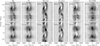 |
Fig. 7. Trailed hydrogen and helium emission line spectra. Left two panels: observed line profiles of Hβ and Hγ. Center two panels: disk component obtained by subtracting the fitted spin component from the observed profiles (see text). The emission of this component stays between the two vertical dashed lines at υterm = ±1200 km s−1. Right two panels: trailed line spectra of He Iλ4471 and HeII [[INLINE178]]. These are disturbed by Mg IIλ4481 and He I λ4713 centered at +650 km s−1 and +1750 km s−1, respectively. |
3.5. Decomposition of He Iλ4471 and He IIλ4686
The two right panels in Fig. 7 show the complex continuum-subtracted trailed spectra of He Iλ4471 and He IIλ4686. Both are heavily disturbed by competing lines, He II by He Iλ4713 at a separation of +27 Å and He Iλ4471 by a previously unrecognized contamination by Mg IIλ4481 at +10 Å.
Despite the heavy contamination, applying the model of Eq. (5) to the He Iλ4471 spectra at orbital phases ϕ98 = 0.0 and 0.30 (Fig. 7) provides some important information. The spin-modulated component extends only to wavelengths of ±2100 km s−1 (upper right panel of Fig. 5), much less than found for the Balmer lines or He IIλ4686. Since the extreme wings of all lines originate primarily from photoionization deep in the magnetospheric accretion curtain or funnel, the difference between the helium lines is likely the result of the ionization structure in the funnel: helium exists almost entirely as He II close to the WD and increasingly as He I farther out. The central low-velocity part of the He I lines originates in part from collisional ionization and photoionization in the disk, leading to a double-peak structure similar to that in the Balmer lines. This does not hold for He IIλ4686, however.
As has long been known, the line profile of He IIλ4686 differs from the Balmer and He I lines, being single peaked, with a base width of at least 6000 km s−1, comparable to that of the Balmer lines. The He II line lacks the double peaks of disk origin and the low-velocity absorption between ϕ98 = 0.6 and 0.9 that is prominent in the Balmer and He I lines (white patches in Fig. 7). Such absorption patches are seen in the He II trailed spectrum at +1750 km s−1; they are created by He Iλ4713. Nevertheless, there is a weak component of disk origin also in He IIλ4686 in the form of S-wave emission from the bulge on the disk at ϕ98 ≃ 0.65 (Fig. 7). At ϕ98 ≃ 0.30 an almost undisturbed spin component of the He II line is observed, which can be analyzed with Eq. (5). The lower right panel of Fig. 5 shows the spectrum at spin maximum (black) and spin minimum (blue) together with the multiples of the spin modulation, fitted over ±3000 km s−1 (red). With Cmax = 2.54 and Cmin = 1.54, He II has a smaller relative spin amplitude than the Balmer lines. In this case, the entire line profiles at spin maximum and minimum are proportional to each other. Hence, by Eq. (5) there is no discernible disk component at ϕ98 = 0.30 (green). The Balmer and He II spin profiles agree in the wings, but differ drastically between ±1200 km s−1. We conjecture that differences in the radiative transfer are responsible. Pushed up matter at the inner edge of the disk may prevent soft X-rays from reaching the surface of the thin disk, but not the pushed-up matter at the outer edge of the disk where the S-wave is produced. At an inclination of 78°, Balmer line emission from the disk passes through denser parts of the bulge closer to the orbital plane than He II photons from the vicinity of the WD. Hence, the He II line may more closely correspond to the intrinsic spin profile than the spin templates of Fig. 6. Kim & Beuermann (1996) showed that single-peaked line profiles occurred in their model calculations, but the remaining systematic uncertainties prevented definite conclusions.
3.6. Doppler tomography
We subjected the combined trailed spectra of both observing nights in Figs. 1 and 7 to a tomographic analysis by fast maximum entropy Doppler imaging, which combines the advantages of the maximum entropy method with the speed of filtered back-projection inversion (Spruit 1998). The results are displayed in Figs. 1 and 8. A bin size of 20 km s−1 was chosen, which corresponds to 1.1 spectral bins of 0.3 Å in the observed spectra. The origin of the coordinate system is at the center of gravity (plus sign), the WD is at υy = −59 km s−1 (bullet). The Roche lobe of the secondary star is based on the system parameters of Sect. 3.7, and is shown as the thick solid curve in all tomograms. The dashed and dot-dashed curves in Fig. 8 describe the single-particle trajectory in velocity space and the Kepler velocity along that trajectory, respectively. The solid circle, which is centered on the WD, denotes the line-of-sight component of the Kepler velocity at the circularization radius. It is based on the fit of Hessman & Hopp (1990) to the calculations of Lubow & Shu (1975), which also account for the gravitational pull of the secondary star, rcirc/a = 0.0859q−0.426, with a the binary separation. For a mass ratio q = M2/M1 = 0.137 (Sect. 3.7) the circularization radius is rcirc = 0.200 a = 9.44 × 109 cm. The Kepler velocity at rcirc is υkep(rcirc) = 1055 km s−1, with a line-of-sight component of 1032 km s−1 for an inclination  (Sect. 3.7).
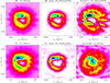 |
Fig. 8. Orbital tomograms of emission lines of EX Hya. Top, from left: (1) Tomogram of the observed Hβ spectra, (2) Tomogram of the disk component of Hβ after subtraction of the spin-modulated component, (3) Tomogram of the observed spectra of He Iλ4471. Bottom, from left: (4) Tomogram of the observed Hγ spectra, (5) Tomogram of the disk component of Hγ, (6) Tomogram of the observed spectra of He IIλ4686. In each panel the dashed curve indicates the single-particle trajectory and the dot-dashed curve the Kepler velocity along that path. The solid circle denotes the velocity at the circularization radius, shifted by −59 km s−1 in υy to be centered on the WD. The color scale is as follows: white = 0.0, magenta ≃ 0.10, red ≃ 0.25, yellow ≃ 0.40, green ≃ 0.55, cyan ≃ 0.70, light blue ≃ 0.80, dark blue ≃ 0.90, black = 1.0. |
We used smoothing parameters that avoid spokes as much as possible, without losing important structure. Spokes are prominent in the tomogram of He Iλ4471, but less so in the others. Trailed spectra that vary at two frequencies are not provided for in standard tomography, and if analyzed at either frequency, one of them is incorrectly represented (Hellier 1999). As noted in Sect. 3.4, the trailed spectra of the spin component contain no sinusoidal structure or part thereof that the tomogram can assign to a specific position in velocity space. No information is obtained from these tomograms and we do not show them.
The orbital tomography of the narrow emission lines of Fe Iλ4957 and Ca IIλ8498 in Fig. 1 proves their origin from the heated face of the secondary star. Our measurement of the velocity amplitude of the secondary star, K2 = 432.4 ± 4.8 km s−1 (Paper I, BR08), rested on the interpretation of the Ca IIλ8498 line profiles in terms of an advanced illumination model.
3.6.1. Orbital tomograms of the observed trailed spectra
The orbital tomograms of the observed spectra of Hβ and Hγ in Fig. 7 are shown in the two left panels of Fig. 8. They compare well with the results of Belle et al. (2005), Mhlahlo et al. (2007), and Echevarría et al. (2016), except that the emission of the irradiated secondary star is not seen in their data. These tomograms include the azimuthally smeared out spin component at high velocities, which merges with the central representation of the disk features, masking the transition between the two.
The tomogram of He Iλ4471 is shown in the upper right panel of Fig. 8. As Hβ, it extends to high velocities. Part of the enhanced emission around velocities of 1200 km s−1 is an artifact produced by the Mg IIλ4481 line that creates a false impression of the transition between the disk and spin components.
The He II spectra are single peaked and the intensity of the tomogram is centered on the WD. The He II tomogram in the lower right panel of Fig. 8 is representative of the emission in the inner part of the accretion curtains seemingly with little interference by emission or absorption by matter in the disk. The radial profile of the emission may be affected, however, by the varying degree of helium ionization. Many details of the complex radiative transfer in the magnetosphere and disk bulge remain to be studied (Ferrario et al. 1993; Kim & Beuermann 1996). A peculiar feature in the He II tomogram is an emission peak in the vicinity of L1 that could arise from matter lingering in front of L1. Stellar prominences, as observed in QS Vir, provide a possible explanation (Parsons et al. 2011). Artifacts created by He Iλ4713 are the long whitish arc in the lower left and the emission patch around υx, υy ≃ +500, −1000 km s−1.
3.6.2. Tomography of the disk component
The tomograms of the core components of Hβ and Hγ are displayed in the two central panels of Fig. 8. Their most obvious feature is (i) the strict limitation to velocities below about 1200 km s−1. Additional features include (ii) an asymmetry of the terminal velocity of the disk; (iii) the emission from the ballistic stream and the hot spot; (iv) additional emission from farther downstream, possibly indicating stream overflow, and (v) the emission from the irradiated face of the secondary star. We deal with these topics in turn.
Ad (i): The double-peaked Balmer line profile is mapped into the broad ring of emission that extends from about 500 to beyond 1100 km s−1, vanishing at 1300 km s−1. The last two numbers define the range over which the intensity in the tomogram decreases. Reducing the smoothing parameter does not cause the transition to become significantly sharper, suggesting that there is, in fact, such a transition region. The quoted velocity range corresponds to distances from the WD between 6.0 × 10⁹ and 8.3 × 109 cm or 8.2 − 11.3R1 and 64 − 88% of the circularization radius5. This appears plausible in the diamagnetic blob model of King (1993), which is characterized by non-circular and non-Keplerian motion in the vicinity of rcirc and involves a finite radial transition region over which the individual blobs attach to the magnetic field of the WD. For definiteness, we quote a mean terminal velocity in the transition region of υterm ≃ 1200 km s−1, and an inner radius of the disk rin ≃ 7 × 109 cm or close to 10R1, effectively recovering the result of Hellier et al. (1987).
Ad (ii): The Balmer line emission at the inner edge of the disk is not exactly centered on the WD, but displaced by ∼100 km s−1 toward azimuth ψ ≃ 110°, indicating a slightly non-circular motion at the inner disk rim. Its presence and the observed phasing are as expected from the diamagnetic blob model (King 1993; King & Wynn 1999; Kunze et al. 2001).
Ad (iii): In all tomograms the bright spot is located at υx, υy ≃ −500, +420 km s−1, above the single-particle trajectory, implying that the stream is accelerated azimuthally as it interacts with the Keplerian disk (see also Mhlahlo et al. 2007; Echevarría et al. 2016). SMP model calculations by Kunze et al. (2001) nicely illustrate this process.
Ad (iv): The main topic of Kunze et al. (2001) was the ubiquity of stream overflows in CV disks. Their calculations are helpful in identifying the path of the stream and its re-impact on the disk. In our tomograms, bright regions that follow the hot spot in azimuth may indicate the stream near peak altitude above the disk (υx, υy ≃ −1000, +0 km s−1) and the re-impact on the disk (υx, υy ≃ −100, −700 km s−1).
Ad (v): One of the bright emission peaks in the Hβ tomogram is the irradiated face of the secondary star. In Hγ the secondary is fainter and the hot spot brighter, indicating a steeper Balmer decrement for the chromospheric emission from the secondary star than for the hot spot. The emission from the secondary star is faint in He Iλ4471 and is not detectable in He IIλ4686.
3.7. Orbital velocity of the WD and system parameters
A reliable measurement of K1 from the Balmer line wings requires that the very high positive and negative radial velocities cancel out. Model calculations by Ferrario et al. (1993) showed that almost complete compensation is achieved if the curtains at both poles are permanently visible. This requires a large inner hole of the disk, and results in a net velocity amplitude as low as ∼40 km s−1. The existence of velocity variations at the spin period was indicated by the detection of V/R variations (Hellier et al. 1987; Mhlahlo et al. 2007), but they have not yet been included in the orbital velocity fits.
Our approach differs from that of other authors in two respects: we represented the line wings by appropriate templates rather than Gaussians or Lorentzians, and we accounted explicitly for radial velocity variations at both ϕ98 and ϕ67. In the left panels of Fig. 9 we show the individual radial velocities of Hβ and Hγ of both nights folded over the orbital (top) and the spin period (bottom). A clear modulation exists at both periods, with the large scatter caused by the mutually competing period. The amplitudes are about 60 km s−1 for the orbital and 40 km s−1 for the spin modulation; the latter is as predicted by Ferrario et al. (1993). There is no evidence for variations at Porb/2 or Pspin/2 (Gilliland 1982; Hellier et al. 1987). A much clearer picture is obtained by fitting the mean radial velocities of Hβ and Hγ for each night as a function of time by the sum of two sinusoids varying with ϕ98 and ϕ67,
![$$ \begin{aligned} \upsilon _\mathrm{rad} = K_1\,\mathrm{sin} [2\pi (\phi _{98}-\phi _1)]+K_\mathrm{S} \,\mathrm{cos} [2\pi (\phi _{67}-\phi _\mathrm{S} )]+\gamma , \end{aligned} $$](/articles/aa/full_html/2024/06/aa44473-22/aa44473-22-eq10.gif)
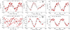 |
Fig. 9. Radial velocities of Hβ and Hγ for the nights of 23 and 26 January 2004. Left panels: individual velocities of Hβ and Hγ for both nights plotted vs. orbital phase (top) and vs. spin phase (bottom). A typical error is shown attached to the open circle. The solid curves represent single sine fits. Center panels: mean radial velocities of Hβ and Hγ for 23 January (top) and 26 January (bottom), fitted by Eq. (7) (solid curve). The dashed and dash-dotted curves indicate the components that vary on the orbital and the spin periods, respectively. Right panels: same, but with the spin-modulated component subtracted. |
with amplitudes K1 and KS, zero crossings ϕ1 and ϕS, and a common γ velocity (center panels of Fig. 9). Data points between ϕ98 ≃ 0.95 and 1.05 (crosses) were excluded from the fit, because they were shown to be affected by the partial eclipse of the emission region (Hellier et al. 1987; Echevarría et al. 2016). As expected when two periodicities contribute to the measurements, the combined radial-velocity curves are not sinusoidal and differ for the two nights. To keep the phases over the 45 orbits between January 23 and 26, we chose the continually progressing phase ϕ98 as an independent variable. The fitted orbital and spin components are individually shown by the dashed and dot-dashed curves, respectively, the sum by the fat solid curve. Subtracting the fitted spin component yields the net orbital variations in the right-hand panels of Fig. 9. The fit parameters are listed in Table 4. The K1 values of the two nights agree within their uncertainties. The weighted mean is K1 = 58.7 ± 3.9 km s−1. The different results for KS may indicate that the ansatz of Eq. (7) still leaves some aspects unaccounted for.
Parameters of a two-component fit to the mean radial velocities of Hβ and Hγ.
There is good agreement between the orbital radial velocity amplitudes K1 of the WD measured from X-ray and far-ultraviolet emission lines that originate on or near the WD, and from the wings of the Balmer emission lines. The first method gave K1 = 58.2 ± 3.7 km s−1 (Hoogerwerf et al. 2004) and 59.6 ± 2.6 km s−1 (Belle et al. 2003), the second 58 ± 5 km s−1 (Echevarría et al. 2016), 58.7 ± 3.9 km s−1 (this work), and similar values in earlier publications (see Table 4 in Echevarría et al. 2016). A weighted mean of the quoted four best-defined amplitudes is K1 = 58.9 ± 1.8 km s−1. Together with the velocity amplitude of the secondary star K2 = 432.4 ± 4.8 km s−1 and an inclination  (BR08), the component masses become M1 = 0.790 ± 0.034 M⊙ and M2 = 0.108 ± 0.007, practically the same as in BR08 and in Echevarría et al. (2016).
3.8. Spin-phase dependence of the eclipse times
Further information that helps to localize the inner disk edge can be gathered from shifts of the optical and X-ray mid-eclipse times in orbital phase. Jablonski & Busko (1985) and Siegel et al. (1989) found that the optical timings shift back and forth by about ±20 s as a function of spin phase, corresponding to a lateral displacement of the centroid of the eclipsed light in the orbital plane of ±109 cm. Siegel et al. (1989) located the emission in the pre-shock region of the magnetically guided accretion stream, while Revnivtsev et al. (2011) and Suleimanov et al. (2016, 2019, and refeences therein) placed it at the inner edge of the accretion disk. Other authors assigned the eclipsed light, at least in part, to the hot spot at the outer edge of the disk. Given that the emission is probably distributed in the projected lateral distance from the WD, a more detailed discussion is in place.
In addition to the 31 mid-eclipse times of Siegel et al. (1989), we made use of the summary of 342 timings compiled by Echevarría et al. (2016) that contains data between 1962 and 2008 in seven subsets. Of these, five pre-1986 data sets offer sufficient spin-phase coverage to allow the necessary detrending for long-term variations of the eclipse times of unknown origin (Jablonski & Busko 1985; Hellier & Sproats 1992). To this end, we subtracted the mean O − C for each subset. The left panel of Fig. 10 shows the spin-phase dependence of the detrended optical O − C with Echevarria’s data as cyan dots and Siegel’s s data as red dots. A sine fit gives an amplitude Δt = 20.0 ± 1.9 s for the combined data, with maximum positive (negative) O − C at ϕ67 = 0.25 (0.75) (solid curve). Individual fits to the six subsets show no significant variation in amplitude or phase between 1962 and 1985. The information for times after 1985 is too meager to allow a conclusion on the long-term behavior of this modulation.
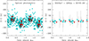 |
Fig. 10. O − C deviations of the mid-eclipse times vs. spin phase. Left: optical eclipse times collected by Echevarría et al. (2016, cyan) and by Siegel et al. (1989, red). The sinusoid fitted to all data has an amplitude of 20 s. Right: X-ray and EUV eclipse times observed with EXOSAT and GINGA (Rosen et al. 1988, 1991, cyan dots) and with the EUVE Deep Survey instrument (Hurwitz et al. 1997; Belle et al. 2002, red dots). |
The right panel of Fig. 10 shows the spin-phase dependence of the extreme ultraviolet (EUV) and X-ray mid-eclipse times, which is based on more scanty data. The eclipse times measured in 1994 and 2000 with the Deep Survey Instrument of the Extreme Ultraviolet Explorer (EUVE) are shown as red dots (Hurwitz et al. 1997; Belle et al. 2002) and the X-ray eclipse times observed in 1985 with the European X-ray Observatory SATellite (EXOSAT) and in 1988 with the Japanese GINGA satellite as cyan dots (Rosen et al. 1988, 1991). We omitted three very ill-defined and uncertain X-ray eclipse times near spin minimum. These mid-eclipse times display no obvious dependence on spin phase, and we conservatively estimate an amplitude Δt < 10s. We interpret the different amplitudes for X-rays and optical light by their respective origin below the strong shock near the WD and farther out in the accretion curtain (see Fig. 11).
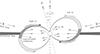 |
Fig. 11. Schematic diagram of the magnetosphere and accretion region as viewed by the observer at spin phase 0.25. The different shades of gray indicate different levels of the mass flow rate Ṁ. Spin maximum occurred 0.25 rotations earlier at ϕ67 = 0 when the upper pole was pointing away from the observer and the lower accretion curtain was most directly in view. |
The observed amplitude Δt reflects the lateral displacement of the centroid of the eclipsed light from the accretion curtain in the lower hemisphere (Beuermann & Osborne 1988)6, ⟨sem⟩≃2π aΔt/Porb at ϕ67 = 0.25 (Fig. 11). The true radial distance rem of the centroid of the eclipsed light may substantially exceed ⟨sem⟩, depending on the azimuthal distribution I(ψ) of the emission. With ψ = 0 in the direction of the observer, the centroid of the emission displays a relative shift ⟨sem⟩/rem = ⟨sin ψ⟩2π, where the right-hand term is the intensity-weighted 2π average. To give an example, we assume that accretion occurs over 2π in azimuth and the emission varies as I(ψ) = 1 + a sin ψ, with a < 1. Then, for example, for a = 2/3 the emission varies by a factor (1 + a)/(1 − a) = 5 between maximum (dark gray) and minimum (light gray) and rem = (2/a)⟨sem⟩ = 3 ⟨sem⟩ or rem ≃ 3 × 109 cm for Δt = 20 s. If the emission is centered halfway between rin and the WD, the example corresponds to rin ≃ 6 × 109 cm, about the value obtained from our tomography.
4. Discussion
4.1. Inner edge of the accretion disk
We decomposed the Hβ and Hγ line profiles into a spin-modulated component that is responsible for the entire line wings and an orbital phase-modulated component that largely represents the accretion disk. Our tomography shows the disk emission to be restricted to υrad ≲ 1200 km s−1, tapering off between 1100 and 1300 km s−1, equivalent to Kepler radii between 6.0 and 8.3 × 109 cm or 8.2 and 11.3R1. In general, we confirm the classical model that was established when EX Hya was recognized as an IP (Kruszewski et al. 1981; Cordova et al. 1985; Hellier et al. 1987; Kaitchuck et al. 1987) and assigns the entire line wings to streaming motions in the magnetosphere.
This model was challenged by Revnivtsev et al. (2009) who interpreted a break in the power spectra of the optical and X-ray temporal fluctuations with the Kepler frequency at the inner edge of the disk, seemingly an elegant method of measuring rin. Applications by Revnivtsev et al. (2011), Semena et al. (2014), and Suleimanov et al. (2016, 2019) gave inner disk radii for EX Hya between 2 and 4R1, implying that velocities in the Balmer line wings up to between 2600 and 1800 km s−1 represent Keplerian motion in the disk and velocities beyond streaming motions in the magnetosphere. This dichotomy is inconsistent with our finding that the entire Balmer line wings at υrad ≳ 1200 km s−1 vary with spin phase as a single component. Furthermore, He II line emission originates almost exclusively from the magnetospheric funnels, and this will hold for strong far-ultraviolet emission lines as Si IVλ1400 as well. It is unlikely that the Balmer line wings behave so differently. A variety of optical and X-ray observations demand that the accretion curtains on the WD in EX Hya be tall and the lower one be visible through the hole in the inner disk. With a required shock height hsh ∼ 1R1 (Allan et al. 1998; Luna et al. 2018), an inner disk radius of about 9R1 is required. If this requirement is violated, the small-magnetosphere model runs into problems, which explains a wide range of observations, including (i) the partial nature of the X-ray eclipse (Beuermann & Osborne 1988; Rosen et al. 1991; Mukai 1998), (ii) the energy dependence of the X-ray spin modulation (Rosen et al. 1991), (iii) the observed shock temperature (Sect. 4.2), (iv) the weak Fe Kα 6.4 keV line and the absence of a strong reflection component in the hard X-ray spectrum (Luna et al. 2018), and (v) the almost complete compensation of the streaming motions from both curtains (Ferrario et al. 1993, and this work). Hence, there is ample evidence for a large inner hole in the accretion disk of EX Hya. We conclude that the model of Revnivtsev et al. (2009) yields an incorrect result, and we agree with Luna et al. (2018), who considered its basic assumption as suspect.
In many IPs at longer orbital periods, rin ≃ rcor, which causes them to accrete near spin equilibrium. The large-magnetosphere model defines the conditions under which EX Hya can be considered to accrete in spin equilibrium (King & Wynn 1999; Norton et al. 2004, 2008). Belle et al. (2002) and Mhlahlo et al. (2007) discussed their data within such a model, but did not quote a value of rin. We discuss this model in Sect. 4.3.
4.2. Shock temperature
The freefall of accreting matter to the WD starts at rin and is braked at the shock at height hsh above its surface. The electron temperature behind a strong shock is given by
where the numerical factor is kTsh = (3/8) μmuGM1/R1 = 34.3 keV; μ = 0.619 is the mean molecular weight for a plasma of solar composition; and mu is the unit mass. We used Mwd = 0.79 M⊙ and R1 = 7.35 × 108 cm (BR08). The published shock temperatures were measured by fitting cooling flow models to the observed hard X-ray spectra. Published values include 12.7 keV (Yuasa et al. 2010), 15.4 keV (Fujimoto & Ishida 1997), 16 keV (Hoogerwerf et al. 2004), 18.0 keV (Hayashi & Ishida 2014), 19.4 keV (Brunschweiger et al. 2009), 19.7 keV (Luna et al. 2018), and ∼20 keV (Mukai et al. 2003).
For rin = 10R1, Eq. (8) reproduces the quoted range of the observed shock temperatures for shock heights of 0.5 − 1.2R1, in agreement with the observationally required hsh ∼ 1.0.
4.3. Magnetic moment of the white dwarf
The magnetic moment μ1 of the WD is directly related to the size of rin. Obtaining an estimate of μ1 is straightforward if we assume that the theory of the interaction of a viscous disk with a magnetosphere (e.g., Ghosh & Lamb 1979, see also White & Stella 1988) is applicable to EX Hya. In this theory, azimuthal magnetic stresses bring the plasma into corotation with the field at a radius

where Kelvin-Helmholtz instabilities cause it to be invaded by the stellar field and accreted (Arons & Lea 1980). Here M1 is the mass of the WD,  its magnetic moment, B1 the surface field strength, Ṁ the accretion rate, and ζ a factor that depends on, among other parameters, the ratio of the angular velocities of field and plasma (fastness parameter). For the parameters of EX Hya, ζ ≃ 0.45 (see also White & Stella 1988). Equating rmag with rin ≃ 7 × 109 cm and using M1 = 0.79 M⊙ and Ṁ = 3.9 × 10⁻¹¹ M⊙yr−1, gives μ1 ≃ 1.3 × 1032 Gcm3 and B1 ≃ 0.35 MG. With a polar field strength of less than 1 MG, no optical circular polarization is expected. The quoted Ṁ is based on the overall spectral energy distribution of Eisenbart et al. (2002) that we updated and converted to spin maximum. Its integrated flux, Facc = 8.2 × 10⁻¹⁰ erg cm−2s−1, represents our best estimate of the 4π-averaged emission of EX Hya, and leads to the quoted Ṁ at d = 56.77 pc (Bailer-Jones et al. 2021). The result agrees closely with the mass transfer rate expected from gravitational radiation and the spin-up of the WD (Ritter 1985).
It is instructive to consider the condition under which EX Hya might be able to synchronize. It requires that the magnetic torque Gmag = γ μ1 μ2 /a3 g cm2s−2 exceeds the accretion torque Gacc =Ṁ(GM1rmag)1/2 g cm2s−2, where  is the magnetic moment of the secondary star, B2 and R2 are its field strength and radius, and γ is a geometry-dependent factor of order unity (King et al. 1990). The secondary in EX Hya is taken to possess a dynamo similar to the rapidly rotating field stars studied by Reiners et al. (2009). Stars with Rossby number Ro < 0.10 possess a saturated dynamo that generates a surface field of roughly 3 kG with a scatter of 1 kG. The stars with the lowest Ro ∼ 0.01 have field strengths of around 2 kG, which we adopt tentatively as the field strength of the secondary in EX Hya. With R2 = 1.055 × 1010 cm (BR08), the secondary in EX Hya would then have a magnetic moment μ2 ∼ 2.3 × 1033 G cm3 and the magnetic torque becomes Gmag = 2.9 × 1033γ g cm2s−2, while the accretion torque is Gacc = 2.1 × 1033 g cm2s−2. Hence, the torques are of similar magnitude, and one may speculate that EX Hya was in synchronous rotation in the past, but failed to regain it, for example when Ṁ changed. We recall that the disk emission vanishes at r = 6 × 109 cm, slightly exceeding the radius of closest approach to the WD in ballistic orbits (Lubow & Shu 1975), suggesting that formation of the disk may have been marginal.
In the alternative picture of King (1993) and King & Wynn (1999), the disk in EX Hya consists of diamagnetic blobs that interact individually with the local field through a surface drag, thereby exchanging orbital energy and angular momentum with the stellar components. The interaction proceeds via the emission of Alfvén waves generated as the blobs pass across field lines, and “pluck them as violin strings” (Drell et al. 1965a,b; King 1993). The timescale of this process, tmag ≃ cAρblb/B2, depends on the local field strength, on the Alfvén velocity cA in the inter-blob medium, and on the blob density and size ρb and lb. Complex flow patterns may accrue if blobs with a wide parameter range are present (King & Wynn 1999, their Fig. 4). An overview and a classification of the flow patterns was presented by Norton et al. (2004, 2008). For an intermediate range of WD magnetic moments the flow is either a stream or a propeller, depending on the spin period. A disk-like or a ring-like structure develops at the low or the high end of the μ1 scale, respectively (Norton et al. 2008, their Figs. 1 and 2). The ring-like structure was proposed by King & Wynn (1999) in an attempt to show that conditions exist under which EX Hya may accrete in spin equilibrium. A magnetic moment μ1 > 1035 G cm3 is required for this possibility and a ring is formed at the WD Roche radius or, equivalently, the corotation radius, from which the WD accretes over 360° in azimuth. We can exclude both the high μ1 and the large rin. The second possibility is the disk mode that is realized for μ1 < 3 × 1033 G cm3 at the orbital period of EX Hya. We conclude that EX Hya resides securely in this section of Norton’s zoo. Further study is needed to shed more light on the evolutionary status of EX Hya.
5. Conclusions
Our main results can be summarized as follows:
(1) We decomposed the Balmer line profiles of EX Hya in a unique way into the spin-modulated wings and an orbital-phase modulated core. The former represents the magnetically guided accretion stream; the latter is dominated by the accretion disk.
(2) Tomography of the core component shows a broad ring of emission from the disk and S-wave component, both confined to υkep ≲ 1200 km s−1 or rin ≃ 7 × 109 cm ≃ 10R1 ≃ 0.75 rcirc.
(3) The inner hole of the disk is sufficiently large to permit an unobstructed view of the lower accretion column for shock heights up to hsh ≃ 1.0R1, as required by a wide range of optical and X-ray observations.
(4) We estimated a WD magnetic moment μ1 ≃ 1.3 × 1032 G cm3 and a surface field strength of 0.35 MG. With a polar field strength Bp ≲ 1 MG, no optical circular polarization is expected.
(5) The measured rin excludes the small-magnetosphere model of Revnivtsev et al. (2009), and the estimate of μ1 probably excludes the large-magnetosphere model of King & Wynn (1999). EX Hya is found to accrete far from spin equilibrium.
(6) The similar magnitudes of the magnetostatic and accretion torques suggest conditions possibly close to synchronization.
(7) The orbital velocity amplitude of the WD, K1 = 58.7 ± 3.9 km s−1, agrees perfectly with previous results, confirming the published component masses.
http://astroutils.astronomy.ohio-state.edu/time/ converts UTC to Barycentric Julian Date in Barycentric Dynamical Time BJD (TDB).
The US Department of Commerce National Institute of Standards and Technology: https://www.nist.gov/pml/atomic-spectra-database
The ephemeris of Echevarría et al. (2016) was approximately converted from HJD to BJD (TDB).
Acknowledgments
We thank the anonymous referee for a quick, constructive, and helpful response. We thank Axel Schwope for providing the program for Doppler tomography originally written by Henk Spruit and for numerous enlightening discussions. We thank Stefan Eisenbart for Fig. 10 from his PhD Thesis (Eisenbart 2000).
References
- Allan, A., Hellier, C., & Beardmore, A. 1998, MNRAS, 295, 167 [CrossRef] [Google Scholar]
- Andronov, I. L., & Breus, V. V. 2013, Astrophysics, 56, 518 [NASA ADS] [CrossRef] [Google Scholar]
- Arons, J., & Lea, S. M. 1980, ApJ, 235, 1016 [NASA ADS] [CrossRef] [Google Scholar]
- Bailer-Jones, C. A. L., Rybizki, J., Fouesneau, M., et al. 2021, AJ, 161, 147, VizieR Online Data Catalog: I/352 [NASA ADS] [CrossRef] [Google Scholar]
- Belle, K. E., Howell, S. B., Sirk, M. M., & Huber, E. 2002, ApJ, 577, 359 [NASA ADS] [CrossRef] [Google Scholar]
- Belle, K. E., Howell, S. B., Sion, E. M., Long, K. S., & Szkody, P. 2003, ApJ, 587, 373 [NASA ADS] [CrossRef] [Google Scholar]
- Belle, K. E., Howell, S. B., Mukai, K., et al. 2005, AJ, 129, 1985 [NASA ADS] [CrossRef] [Google Scholar]
- Beuermann, K., & Osborne, J. P. 1988, A&A, 189, 128 [NASA ADS] [Google Scholar]
- Beuermann, K., & Reinsch, K. 2008, A&A, 480, 199 [NASA ADS] [CrossRef] [EDP Sciences] [Google Scholar]
- Bisikalo, D. V., Zhilkin, A. G., Isakova, P. B., et al. 2020, Adv. Space Res., 66, 1057 [NASA ADS] [CrossRef] [Google Scholar]
- Brunschweiger, J., Greiner, J., Ajello, M., et al. 2009, A&A, 496, 121 [NASA ADS] [CrossRef] [EDP Sciences] [Google Scholar]
- Breysacher, J., & Vogt, N. 1980, A&A, 87, 349 [NASA ADS] [Google Scholar]
- Butters, O. W., Katajainen, S., Norton, A. J., et al. 2009, A&A, 496, 891 [NASA ADS] [CrossRef] [EDP Sciences] [Google Scholar]
- Cordova, F. A., Mason, K. O., & Kahn, S. M. 1985, MNRAS, 212, 447 [NASA ADS] [CrossRef] [Google Scholar]
- Cowley, A. P., Hutchings, J. B., & Crampton, D. 1981, ApJ, 246, 489 [NASA ADS] [CrossRef] [Google Scholar]
- Drell, S. D., Foley, H.M., & Ruderman, M.A. 1965a, Phys. Rev. Lett., 14, 171 [NASA ADS] [CrossRef] [Google Scholar]
- Drell, S. D., Foley, H. M., & Ruderman, M. A. 1965b, J. Geophys. Res., 70, 3131 [Google Scholar]
- Eastman, J., Siverd, R., & Gaudi, B. S. 2010, PASP, 122, 935 [Google Scholar]
- Echevarría, J., Ramírez-Torres, A., Michel, R., et al. 2016, MNRAS, 461, 1576 [CrossRef] [Google Scholar]
- Eisenbart, S. 2000, Ph.D. Thesis, Univ. of Göttingen, Germany [Google Scholar]
- Eisenbart, S., Beuermann, K., Reinsch, K., & Gänsicke, B. T. 2002, A&A, 382, 984 [NASA ADS] [CrossRef] [EDP Sciences] [Google Scholar]
- Ferrario, L., Wickramasinghe, D. T., & King, A. R. 1993, MNRAS, 260, 149 [NASA ADS] [Google Scholar]
- Fujimoto, R., & Ishida, M. 1997, ApJ, 474, 774 [NASA ADS] [CrossRef] [Google Scholar]
- Ghosh, P., & Lamb, F. K. 1979, ApJ, 234, 296 [Google Scholar]
- Gilliland, R. L. 1982, ApJ, 258, 576 [NASA ADS] [CrossRef] [Google Scholar]
- Hayashi, T., & Ishida, M. 2014, MNRAS, 441, 3718 [NASA ADS] [CrossRef] [Google Scholar]
- Hellier, C. 1999, ApJ, 519, 324 [NASA ADS] [CrossRef] [Google Scholar]
- Hellier, C., & Sproats, L. N. 1992, IBVS, 3724, 1 [NASA ADS] [Google Scholar]
- Hellier, C., Mason, K. O., Rosen, S. R., & Cordova, F. 1987, MNRAS, 228, 463 [NASA ADS] [CrossRef] [Google Scholar]
- Hessman, F. V., & Hopp, U. 1990, A&A, 228, 387 [Google Scholar]
- Hoogerwerf, R., Brickhouse, N. S., & Mauche, C. W. 2004, ApJ, 610, 411 [NASA ADS] [CrossRef] [Google Scholar]
- Hurwitz, M., Sirk, M., Bowyer, S., & Ko, Y.-K. 1997, ApJ, 477, 390 [NASA ADS] [CrossRef] [Google Scholar]
- Jablonski, F., & Busko, I. C. 1985, MNRAS, 214, 219 [NASA ADS] [CrossRef] [Google Scholar]
- Kaitchuck, R. H., Hantzios, P. A., Kakaletris, P., et al. 1987, ApJ, 317, 765 [CrossRef] [Google Scholar]
- King, A. R. 1993, MNRAS, 261, 144 [NASA ADS] [CrossRef] [Google Scholar]
- King, A. R., & Wynn, G. A. 1999, MNRAS, 310, 203 [NASA ADS] [CrossRef] [Google Scholar]
- King, A. R., Frank, J., & Whitehurst, R. 1990, MNRAS, 244, 731 [NASA ADS] [Google Scholar]
- Kim, Y., & Beuermann, K. 1996, A&A, 307, 824 [NASA ADS] [Google Scholar]
- Kruszewski, A., Mewe, R., Heise, J., et al. 1981, Space. Sci. Rev., 30, 221 [NASA ADS] [CrossRef] [Google Scholar]
- Kunze, S., Speith, R., & Hessman, F. V. 2001, MNRAS, 322, 499 [NASA ADS] [CrossRef] [Google Scholar]
- Lubow, S. H., & Shu, F. H. 1975, ApJ, 198, 38 [Google Scholar]
- Luna, G. J. M., Mukai, K., Orio, M., et al. 2018, ApJ, 852, L8 [NASA ADS] [CrossRef] [Google Scholar]
- Mauche, C. W., Brickhouse, N. S., Hoogerwerf, R., et al. 2009, IBVS, 5876, 1 [NASA ADS] [Google Scholar]
- Mhlahlo, N., Buckley, D. A. H., Dhillon, V. S., et al. 2007, MNRAS, 378, 211 [NASA ADS] [CrossRef] [Google Scholar]
- Mukai, K., Ishida, M., Osborne, J., et al. 1998, ASP Conf. Ser., 137, 554 [NASA ADS] [Google Scholar]
- Mukai, K., Kinkhabwala, A., Peterson, J. R., et al. 2003, ApJ, 586, L77 [NASA ADS] [CrossRef] [Google Scholar]
- Norton, A. J., Wynn, G. A., & Somerscales, R. V. 2004, ApJ, 614, 349 [NASA ADS] [CrossRef] [Google Scholar]
- Norton, A. J., Butters, O. W., Parker, T. L., et al. 2008, ApJ, 672, 524 [NASA ADS] [CrossRef] [Google Scholar]
- Parsons, S. G., Marsh, T. R., Gänsicke, B. T., et al. 2011, MNRAS, 412, 2563 [NASA ADS] [CrossRef] [Google Scholar]
- Reiners, A., Basri, G., & Christensen, U. R. 2009, ApJ, 697, 373 [NASA ADS] [CrossRef] [Google Scholar]
- Revnivtsev, M., Churazov, E., Postnov, K., et al. 2009, A&A, 507, 1211 [CrossRef] [EDP Sciences] [Google Scholar]
- Revnivtsev, M., Potter, S., Kniazev, A., et al. 2011, MNRAS, 411, 1317 [NASA ADS] [CrossRef] [Google Scholar]
- Ritter, H. 1985, A&A, 148, 207 [NASA ADS] [Google Scholar]
- Rosen, S. R., Mason, K. O., & Córdova, F. A. 1988, MNRAS, 231, 549 [NASA ADS] [CrossRef] [Google Scholar]
- Rosen, S. R., Mason, K. O., Mukai, K., et al. 1991, MNRAS, 249, 417 [CrossRef] [Google Scholar]
- Sarazin, M., & Roddier, F. 1990, A&A, 227, 294 [NASA ADS] [Google Scholar]
- Semena, A. N., Revnivtsev, M. G., Buckley, D. A. H., et al. 2014, MNRAS, 442, 1123 [Google Scholar]
- Siegel, N., Reinsch, K., Beuermann, K., et al. 1989, A&A, 225, 97 [Google Scholar]
- Spruit, H. C. 1998, arXiv e-prints [arXiv:astro-ph/9806141] [Google Scholar]
- Sterken, C., Vogt, N., Freeth, R., et al. 1983, A&A, 118, 325 [NASA ADS] [Google Scholar]
- Suleimanov, V., Doroshenko, V., Ducci, L., et al. 2016, A&A, 591, A35 [NASA ADS] [CrossRef] [EDP Sciences] [Google Scholar]
- Suleimanov, V. F., Doroshenko, V., & Werner, K. 2019, MNRAS, 482, 3622 [NASA ADS] [CrossRef] [Google Scholar]
- Vogt, N., Krzeminski, W., & Sterken, C. 1980, A&A, 85, 106 [NASA ADS] [Google Scholar]
- Warner, B., & McGraw, J. T. 1981, MNRAS, 196, 59P [NASA ADS] [CrossRef] [Google Scholar]
- White, N. E., & Stella, L. 1988, MNRAS, 231, 325 [NASA ADS] [CrossRef] [Google Scholar]
- Yuasa, T., Nakazawa, K., Makishima, K., et al. 2010, A&A, 520, A25 [NASA ADS] [CrossRef] [EDP Sciences] [Google Scholar]
All Tables
Sine fits to narrow-line radial velocities using the (Hellier & Sproats 1992; HS92) linear orbital ephemeris as reference.
Observed times of events quoted as BJD (TDB) with errors, and time predicted by either the linear eclipse ephemeris of Hellier & Sproats (1992) or the quadratic ephemeris for the spin maxima of Mauche et al. (2009, their Eq. (1)).
All Figures
|
Fig. 1. VLT/UVES narrow emission line spectra of Fe Iλ4957 and Ca IIλ8498 observed on 23 and 26 January 2004. Left: grayscale representations of the trailed spectra. Spectral flux increases from white to black. For convenience, the data are shown twice. Right: corresponding tomograms with the Roche lobe contour of the secondary star based on the system parameters of Sect. 3.7 demonstrate the origin from the irradiated face of the secondary star. The relative intensity goes from white (0.0) to black (1.0). The origin of the coordinate system is at the center of gravity. |
| In the text | |
|
Fig. 2. Flux-calibrated spin light curves of the integrated Hβ line flux. The orbital phases are given in the figure. The colored dots indicate the same phase bins as in the left panel. |
| In the text | |
|
Fig. 3. Phase-space coverage of our 51 exposures in the ϕ67–ϕ98 plane. The spectra selected for the spectral decomposition at ϕ98 ≃ 0.30, 0.65, and 1.00 are marked by magenta, blue, and red dots respectively. |
| In the text | |
|
Fig. 4. Flux-calibrated blue spectra taken on 23 and 26 January 2004. Left: grayscale representation of the first night, with spectral flux increasing from white to black. Right: mean spectra of the Hγ to Hβ spectral region at spin maximum (black) and spin minimum (blue) for the orbital phases noted in the figure. The best-fit continua that represent the lower envelope to the spectra are shown as magenta curves. The spin modulation of the emission-line component is shown in red. |
| In the text | |
|
Fig. 5. Hβ and Hγ spin maximum and minimum spectra (black and blue, respectively) at ϕ98 = 0.30, 0.65, and 1.0 (six left-most panels). Overplotted are the fitted spin-modulated components fmod(λ) from Eq. (4) with amplitudes Cmax and Cmin (red). Below, the derived disk component is shown (green). The two right panels show the decomposition of the He Iλ4471 line at ϕ98 = 0.0 and 0.30 and of He IIλ4686 at ϕ98 = 0.30. No He II emission from the disk is seen, but S-wave emission is present at other orbital phases (see text). |
| In the text | |
|
Fig. 6. Mean templates of the spin-modulated component of Hβ and Hγ. |
| In the text | |
|
Fig. 7. Trailed hydrogen and helium emission line spectra. Left two panels: observed line profiles of Hβ and Hγ. Center two panels: disk component obtained by subtracting the fitted spin component from the observed profiles (see text). The emission of this component stays between the two vertical dashed lines at υterm = ±1200 km s−1. Right two panels: trailed line spectra of He Iλ4471 and HeII [[INLINE178]]. These are disturbed by Mg IIλ4481 and He I λ4713 centered at +650 km s−1 and +1750 km s−1, respectively. |
| In the text | |
|
Fig. 8. Orbital tomograms of emission lines of EX Hya. Top, from left: (1) Tomogram of the observed Hβ spectra, (2) Tomogram of the disk component of Hβ after subtraction of the spin-modulated component, (3) Tomogram of the observed spectra of He Iλ4471. Bottom, from left: (4) Tomogram of the observed Hγ spectra, (5) Tomogram of the disk component of Hγ, (6) Tomogram of the observed spectra of He IIλ4686. In each panel the dashed curve indicates the single-particle trajectory and the dot-dashed curve the Kepler velocity along that path. The solid circle denotes the velocity at the circularization radius, shifted by −59 km s−1 in υy to be centered on the WD. The color scale is as follows: white = 0.0, magenta ≃ 0.10, red ≃ 0.25, yellow ≃ 0.40, green ≃ 0.55, cyan ≃ 0.70, light blue ≃ 0.80, dark blue ≃ 0.90, black = 1.0. |
| In the text | |
|
Fig. 9. Radial velocities of Hβ and Hγ for the nights of 23 and 26 January 2004. Left panels: individual velocities of Hβ and Hγ for both nights plotted vs. orbital phase (top) and vs. spin phase (bottom). A typical error is shown attached to the open circle. The solid curves represent single sine fits. Center panels: mean radial velocities of Hβ and Hγ for 23 January (top) and 26 January (bottom), fitted by Eq. (7) (solid curve). The dashed and dash-dotted curves indicate the components that vary on the orbital and the spin periods, respectively. Right panels: same, but with the spin-modulated component subtracted. |
| In the text | |
|
Fig. 10. O − C deviations of the mid-eclipse times vs. spin phase. Left: optical eclipse times collected by Echevarría et al. (2016, cyan) and by Siegel et al. (1989, red). The sinusoid fitted to all data has an amplitude of 20 s. Right: X-ray and EUV eclipse times observed with EXOSAT and GINGA (Rosen et al. 1988, 1991, cyan dots) and with the EUVE Deep Survey instrument (Hurwitz et al. 1997; Belle et al. 2002, red dots). |
| In the text | |
|
Fig. 11. Schematic diagram of the magnetosphere and accretion region as viewed by the observer at spin phase 0.25. The different shades of gray indicate different levels of the mass flow rate Ṁ. Spin maximum occurred 0.25 rotations earlier at ϕ67 = 0 when the upper pole was pointing away from the observer and the lower accretion curtain was most directly in view. |
| In the text | |
Current usage metrics show cumulative count of Article Views (full-text article views including HTML views, PDF and ePub downloads, according to the available data) and Abstracts Views on Vision4Press platform.
Data correspond to usage on the plateform after 2015. The current usage metrics is available 48-96 hours after online publication and is updated daily on week days.
Initial download of the metrics may take a while.