| Issue |
A&A
Volume 683, March 2024
|
|
|---|---|---|
| Article Number | A196 | |
| Number of page(s) | 19 | |
| Section | Extragalactic astronomy | |
| DOI | https://doi.org/10.1051/0004-6361/202347831 | |
| Published online | 18 March 2024 | |
Bars and boxy/peanut bulges in thin and thick discs
III. Boxy/peanut bulge formation and evolution in the presence of thick discs
1
Max-Planck-Institut für Astronomie, Königstuhl 17, 69117 Heidelberg, Germany
e-mail: This email address is being protected from spambots. You need JavaScript enabled to view it.
2
Institute for Computational Cosmology, Department of Physics, Durham University, South Road, Durham DH1 3LE, UK
3
GEPI, Observatoire de Paris, PSL Research University, CNRS, Place Jules Janssen, 92195 Meudon, France
4
Inter-University Centre for Astronomy and Astrophysics, Post Bag 4, Ganeshkhind, Pune, Maharashtra 411007, India
Received:
30
August
2023
Accepted:
6
December
2023
Abstract
Boxy/peanut (b/p) bulges, the vertically extended inner parts of bars, are ubiquitous in barred galaxies in the local Universe, including our own Milky Way. At the same time, the majority of external galaxies and the Milky Way also possess a thick disc. However, the dynamical effect of thick discs in the b/p formation and evolution is not fully understood. Here, we investigate the effect of thick discs in the formation and evolution of b/ps by using a suite of N-body models of (kinematically cold) thin and (kinematically hot) thick discs. Within the suite of models, we systematically vary the mass fraction of the thick disc, and the thin-to-thick disc scale length ratio. The b/ps form in almost all our models via a vertical buckling instability, even in the presence of a massive thick disc. The thin disc b/p is much stronger than the thick disc b/p. With an increasing thick-disc mass fraction, the final b/p structure becomes progressively weaker in strength and larger in extent. Furthermore, the time interval between the bar formation and the onset of buckling instability becomes progressively shorter with an increasing thick-disc mass fraction. The breaking and restoration of the vertical symmetry (during and after the b/p formation) show a spatial variation – the inner bar region restores vertical symmetry rather quickly (after the buckling), while in the outer bar region the vertical asymmetry persists long after the buckling happens. Our findings also predict that at higher redshifts, when discs are thought to be thicker, b/ps would have a more “boxy” appearance than an “X-shaped” one. This remains to be tested in future observations at higher redshifts.
Key words: methods: numerical / galaxies: evolution / galaxies: kinematics and dynamics / galaxies: spiral / galaxies: structure
© The Authors 2024
 Open Access article, published by EDP Sciences, under the terms of the Creative Commons Attribution License (https://creativecommons.org/licenses/by/4.0), which permits unrestricted use, distribution, and reproduction in any medium, provided the original work is properly cited.
This article is published in open access under the Subscribe to Open model.
Open access funding provided by Max Planck Society.
1. Introduction
A number of observational studies find that nearly half of all edge-on disc galaxies in the local Universe exhibit a prominent boxy or peanut-shaped structure (hereafter b/p structure; e.g. see Bureau & Freeman 1999; Lütticke et al. 2000; Erwin & Debattista 2017). A wide variety of observational and theoretical evidence indicates that many bars are vertically thickened in their inner regions, appearing as “boxy” or “peanut-shaped” bulges when seen in edge-on configuration (e.g. Combes & Sanders 1981; Raha et al. 1991; Erwin & Debattista 2016). The presence of b/p structure has also been detected for galaxies in the face-on configurations, for example, in IC 5240 (Buta 1995), IC 290 (Buta & Crocker 1991), and several others (see examples in Quillen et al. 1997; McWilliam & Zoccali 2010; Laurikainen et al. 2011; Erwin & Debattista 2013). Several photometric and spectroscopic studies of the Milky Way bulge revealed that the Milky Way also has an inner b/p structure (e.g. see Nataf et al. 2010; Shen et al. 2010; Ness et al. 2012; Wegg & Gerhard 2013; Wegg et al. 2015). The occurrence of b/p bulges is observationally shown to depend strongly on the stellar mass of the galaxy, and a majority of barred galaxies above stellar mass log(M*/M⊙)≥10.4 host b/p bulges (e.g. see Yoshino & Yamauchi 2015; Erwin & Debattista 2017; Marchuk et al. 2022). A similar (strong) stellar-mass dependence of the b/p bulge occurrence, at redshift z = 0, is shown to exist for the TNG50 suite of cosmological zoom-in simulations (Anderson et al. 2024).
Much of our current understanding of the b/p formation and its growth in barred galaxies is gleaned from numerical simulations. Studies using N-body simulations often find that, soon after the formation of a stellar bar it undergoes a vertical buckling instability, which subsequently gives rise to a prominent b/p bulge (e.g. see Combes et al. 1990; Raha et al. 1991; Merritt & Sellwood 1994; Debattista et al. 2004; Martinez-Valpuesta et al. 2006; Martinez-Valpuesta & Athanassoula 2008; Saha et al. 2013). Indeed, Erwin & Debattista (2016) detected two such local barred-spiral galaxies that are undergoing such a buckling phase. If a barred N-body model is evolved for a long enough time, it might go through a second and prolonged buckling phase, thereby producing a prominent X-shape feature (e.g. Martinez-Valpuesta et al. 2006; Martinez-Valpuesta & Athanassoula 2008). Furthermore, Saha et al. (2013) showed that a bar buckling instability is closely linked with the maximum meridional tilt of the stellar velocity ellipsoid (denoting the meridional shear stress of stars). Alternatively, a b/p bulge can be formed via the trapping of disc stars at vertical resonances during the secular growth of the bar (e.g. see Combes & Sanders 1981; Combes et al. 1990; Quillen 2002; Debattista et al. 2006; Quillen et al. 2014; Li et al. 2023) or by gradually increasing the fraction of bar orbits trapped into this resonance (e.g. see Sellwood & Gerhard 2020). The main difference between these two scenarios of b/p formation is that when the bar undergoes the buckling instability phase, the symmetry about the mid-plane is no longer preserved for a period of time (see discussion in Cuomo et al. 2023).
Regardless of the formation scenario, the b/p bulges are shown to have a significant effect on the evolution of disc galaxies by reducing the bar-driven gas inflow (e.g. see Fragkoudi et al. 2015, 2016; Athanassoula 2016). The formation of b/p bulges can affect metallicity gradients in the inner galaxy (e.g. Di Matteo et al. 2014; Fragkoudi et al. 2017a) and can also lead to bursts in star formation history (e.g. Pérez et al. 2017). In addition, Saha et al. (2018) showed that for a 3D b/p structure (i.e. b/p seen in both face-on and edge-on configurations), it introduces a kinematic pinch in the velocity map along the bar minor axis. Furthermore, Vynatheya et al. (2021) demonstrated that for such a 3D b/p structure, the inner bar region rotates slower than the outer bar region.
On the other hand, a thick-disc component is now known to be ubiquitous in majority of external galaxies as well as in the Milky Way (e.g. see Tsikoudi 1979; Burstein 1979; Yoachim & Dalcanton 2006; Comerón et al. 2011a,b, 2018). The existence of this thick-disc component covers the whole range of the Hubble classification scheme, from early-type S0 galaxies to late-type galaxies (Pohlen et al. 2004; Yoachim & Dalcanton 2006; Comerón et al. 2016, 2019; Kasparova et al. 2016; Pinna et al. 2019a,b; Martig et al. 2021; Scott et al. 2021). The thick-disc component is vertically more extended and kinematically hotter as compared to the thin-disc component. The dynamical role of a thick-disc on the formation and growth of non-axisymmetric structures has been been studied for bars (e.g., Klypin et al. 2009; Aumer & Binney 2017; Ghosh et al. 2023) and spirals (Ghosh & Jog 2018, 2022). Past studies demonstrated that the (cold) thin and (hot) thick discs are mapped differently in the bar and boxy/peanut bulge (e.g. Athanassoula et al. 2017; Fragkoudi et al. 2017b; Debattista et al. 2017; Buck et al. 2019). Since the presence of a thick disc can significantly affect the formation, evolution, and properties of bars (Ghosh et al. 2023), we need to explore how it will affect the b/ps, since b/ps are essentially the vertical extended part of the bar.
Stellar bars are known to be present in high-redshift (z ∼ 1) galaxies (e.g. see Sheth et al. 2008; Elmegreen et al. 2004; Jogee et al. 2004; Guo et al. 2023; Le Conte et al. 2023). Furthermore, a recent study by Kruk et al. (2019) showed the existence of b/p structure in high redshift (z ∼ 1) galaxies as well. At high redshift, discs are known to be thick, kinematically hot (and turbulent), and more gas rich. So, the question remains as to how efficiently the b/p structures can form in such thick discs at such high redshifts. Fragkoudi et al. (2017b) studied the effect of such a thick disc component on the b/p formation using a fiducial two-component thin+thick disc model where the thick disc constitutes 30% of the total stellar mass. The formation and properties of b/p bulges in multi-component discs (i.e. with a number of disc populations greater than two) was also studied in Di Matteo (2016), Debattista et al. (2017), Fragkoudi et al. (2018a,b), and Di Matteo et al. (2019). However, a systematic study of b/p formation in discs with different thin and thick discs, as well as composite thin and thick discs is still missing. We aim to pursue this here.
In this work, we systematically investigated the dynamical role of the thick-disc component in b/p formation and growth using a suite of N-body models with (kinematically hot) thick and (kinematically cold) thin discs. We varied the thick-disc mass fraction and considered different geometric configurations (varying ratio of thin- and thick-disc scale lengths) within the suite of N-body models. We quantified the strength and growth of the b/p in both the thin- and thick-disc stars and studied the vertical asymmetry associated with the vertical buckling instability. In addition, we investigated the kinematic phenomena (i.e. change in the velocity dispersion, meridional tilt angle) associated with the b/p formation and its subsequent growth.
The rest of the paper is organised as follows. Section 2 provides a brief description of the simulation setup and the initial equilibrium models. Section 3 quantifies the properties of the b/p structure, their temporal evolution, and the vertical asymmetry in different models and the associated temporal evolution. Section 4 provides the details of kinematic phenomena related to the b/p formation and its growth, while Sect. 5 provides the details of the relative contribution of the thin disc in supporting the X-shape structure. Section 6 contains the discussion, while Sect. 7 summarises the main findings of this work.
2. Simulation setup, and N-body models
To motivate our study, we used a suite of N-body models consisting of a thin and a thick stellar disc, and the whole system is embedded in a live, dark-matter halo. One such model was already presented in Fragkoudi et al. (2017b). In addition, these models have been thoroughly studied in a recent work of Ghosh et al. (2023) in connection with a bar-formation scenario under varying thick-disc mass fractions. Here, we used the same suite of thin+thick models to investigate b/p formation and evolution with varying thick-disc mass fractions.
The details of the initial equilibrium models and how they are generated are already given in Fragkoudi et al. (2017b) and Ghosh et al. (2023). Here, for the sake of completeness, we briefly mention the equilibrium models. Each of the thin and thick discs is modelled with a Miyamoto-Nagai profile (Miyamoto & Nagai 1975), with Rd, zd, and Md being the characteristic disc scale length, the scale height, and the total mass of the disc, respectively. The dark-matter halo is modelled with a Plummer sphere (Plummer 1911), with RH and Mdm being the characteristic scale length and the total halo mass, respectively. The values of the key structural parameters for the thin and thick discs, dark-matter halo, and the total number of particles used to model each of these structural components are mentioned in Table 1. For this work, we analysed a total of 19 N-body models (including one pure thin-disc-only and three pure thick-disc-only models) of such thin+thick discs.
Key structural parameters for the equilibrium models.
The initial conditions of the discs are obtained using the iterative method algorithm (see Rodionov et al. 2009). For further details, the reader is referred to Fragkoudi et al. (2017b) and Ghosh et al. (2023). The simulations are run using a TreeSPH code by Semelin & Combes (2002). A hierarchical tree method (Barnes & Hut 1986) with opening angle θ = 0.7 is used to calculate the gravitational force, which includes terms up to the quadrupole order in the multipole expansion. A Plummer potential was employed for softening the gravitational forces with a softening length ϵ = 150 pc. We evolved all the models for a total time of 9 Gyr.
Within the suite of thin+thick disc models, we considered three different scenarios for the scale lengths of the two disc (thin and thick) components. In rthickE models, both the scale lengths of thin and thick discs are kept the same (Rd, thick = Rd, thin). In rthickS models, the scale length of the thick-disc component is shorter than that for the thin-disc one (Rd, thick < Rd, thin), and in rthickG models, the scale length of the thick-disc component is larger than that for the thin-disc one (Rd, thick > Rd, thin). Following the nomenclature scheme used in Ghosh et al. (2023), any thin+thick model is referred to as a unique string “[MODEL CONFIGURATION][THICK DISC FRACTION]”. [MODEL CONFIGURATION] denotes the corresponding thin-to-thick disc scale length configuration, that is, rthickG, rthickE, or rthickS, whereas [THICK DISC FRACTION] denotes the fraction of the total disc stars that are in the thick-disc population (or equivalently the mass fraction in the thick-disc as all the disc particles have same mass).
Before we present the results, we mention that in our thin+thick models, we can identify and separate, by construction, which stars are members of the thin-disc component at initial time (t = 0) and which stars are members of the thick-disc component at t = 0, and we can track them as the system evolves self-consistently. Thus, throughout this paper, we refer to the b/p as seen exclusively in particles initially belonging to the thin-disc population as the “thin-disc b/p” and that seen exclusively in particles initially belonging to the thick-disc population as the “thick-disc b/p”.
3. Boxy/peanut formation and evolution for different mass fraction of thick-disc population
3.1. Quantifying the b/p properties
Figure 1 shows the distribution of all stars (thin+thick) in the edge-on projection, calculated at the end of the simulation run (t = 9 Gyr), for all the thin+thick models considered here. In each case, the bar is placed in the side-on configuration (i.e. along the x-axis). A prominent b/p structure is seen in most of these thin+thick models. We further checked the same edge-on stellar density distribution, calculated for the thin- and thick-disc stars separately. Both of them show a prominent b/p structure in most of the thin+thick models. For the sake of brevity, we do not show it here (however, see Fig. 2 in Fragkoudi et al. 2017b).
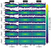 |
Fig. 1. Edge-on density distribution of all disc particles (thin+thick) at the end of the simulation run (t = 9 Gyr) for all thin+thick disc models with varying fthick values. Black dotted lines denote the contours of constant density. Left panels show the density distribution for the rthickS models, whereas middle panels and right panels show the density distribution for the rthickE and rthickG models, respectively. The thick disc fraction (fthick) varies from 0.1 to 1 (top to bottom), as indicated in the left-most panel of each row. The bar is placed along the x-axis (side-on configuration) for each model. The vertical black dashed lines denote the extent of the b/p structure in each case (for details, see the text in Sect. 3.1.2). |
3.1.1. Quantifying the b/p strength and its temporal evolution
Here, we quantify the strength of the b/p structure and study its variation (if any) with thick-disc mass fraction. Following Martinez-Valpuesta & Athanassoula (2008) and Fragkoudi et al. (2017b), in a given radial bin of size ΔR (= 0.5 kpc), we calculate the median of the absolute value of the distribution of particles in the vertical (z) direction,  (normalised by the initial value,
  ) of a snapshot seen edge-on and with the bar placed side-on (along the x-axis). In Fig. 2, we show one example of the corresponding radial profiles of the
  (i = thin, thick, thin+thick) computed separately for the thin- and thick-disc particles, as well as for the thin+thick disc particles, as a function of time. As seen in Fig. 2, a prominent peak in the radial profiles (at later times) of
  denotes the formation of a b/p structure in the thin+thick model. Here, we mention that as the vertical scale height, and hence the vertical extent of thick disc is larger (by a factor of three) than that for the thin disc (see Table 1); the normalisation by
  is necessary to unveil the intrinsic vertical growth due to the b/p formation. When only the absolute values of
  are considered, the thick-disc stars always produce a larger value of
  than the thin-disc stars. This happens due to the construction of equilibrium thin+thick models, and not due to the b/p formation. The normalised peak for the thin-disc is much larger than that for the thick-disc, in concordance with the previous results (Fragkoudi et al. 2017b). Furthermore, at later times, the peak in
  profiles shifts towards outer radial extent (more prominent for the thin disc b/p), indicating the growth of the b/p structure towards outer radial extent. These trends are also seen to hold for other thin+thick models that form a b/p structure during their evolutionary pathway.
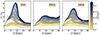 |
Fig. 2. Radial profiles of median of absolute value of distribution of particles in vertical (z) direction, |


To quantify the temporal evolution of the b/p strength, we define the b/p strength at time t, Sb/p(t) as the maximum of the peak value of the  , i.e.,
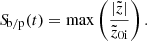 (1)
(1)
In Martinez-Valpuesta et al. (2006) and Martinez-Valpuesta & Athanassoula (2008), a method based on the Fourier decomposition was formulated to quantify the strength of a b/p structure. In Appendix A, we compare this method with Eq. (1) for the thin+thick model rthickE0.5.
Figure 3 shows the corresponding temporal evolution of the b/p strength, calculated separately for the thin and thick discs and for the composite thin+thick disc particles for all thin+thick models considered here. The thin-disc b/p remains much stronger than the thick-disc b/p structure, and this trend holds true for all thin+thick models with three different configurations (i.e. rthickS, rthickE, and rthickG) that develop a prominent b/p structure during their course of temporal evolution.
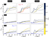 |
Fig. 3. Temporal evolution of b/p strength, Sb/p, calculated using Eq. (1), for thin-disc (upper panels), thick-disc (middle panels), and total (thin+thick) disc stars (lower panels) for all thin+thick disc models with varying fthick values (see the colour bar). Left panels show the b/p strength evolution for the rthickS models, whereas middle panels and right panels show the b/p strength evolution for the rthickE and rthickG models, respectively. The thick disc fraction (fthick) varies from 0.1 to 0.9 (with a step-size of 0.2), as indicated in the colour bar. The blue solid lines in the middle and the bottom rows denote the three thick-disc-only models (fthick = 1), whereas the red solid line in the top middle panel denotes the thin-disc-only model (fthick = 0; for details, see text). |
The temporal evolution of the b/p strength in three thick-disc-only models merits some discussion. For the rthickS1.0 model, the values of Sb/p show a monotonic increase with time, denoting the formation of a prominent b/p structure (also see the bottom row of Fig. 1). However, the final b/p strength for the rthickS1.0 model remains lowest when compared to other rthickS models with different fthick values. For the rthickE1.0 model, the temporal evolution of Sb/p shows a sudden jump around t = 6.5 Gyr and then remains constant. By the end of the simulation, this model forms a b/p structure which appears boxier than a peanut or X shape. For the rthickG1.0 model, the temporal evolution of Sb/p does not show much increment, and the model does not form a prominent b/p structure at the end of the simulation.
In addition, for a fixed value of fthick, we calculated the gradient of Sb/p(t) with respect to time t (dSb/p(t)/dt) for three different geometric configurations considered here. One such example is shown in Fig. 4 for fthick = 0.5. A prominent (positive) peak in the dSb/p/dt profile denotes the onset of the b/p formation. As seen clearly, for a fixed fthick value, the peak in the dSb/p/dt profile occurs at an earlier epoch when compared with the other two geometric configurations. This confirms that the b/p forms at an earlier time in the rthickS0.5 model compared to the rthickE0.5 and rthickG0.5 models. These trends are in tandem with the fact that the bars in rthickS models form at earlier times and grow faster compared to the other two disc configurations (for details, see Ghosh et al. 2023).
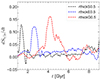 |
Fig. 4. Growth rate of b/p, dSb/p/dt, as a function of time for three thin+thick models with fthick = 0.5. All the stellar particles (thin+thick) are considered here in each model. The growth rate is steeper in rthickS0.5 model when compared with that for other two configurations with same fthick value. |
Lastly, in Fig. 5 (top panel), we show the final b/p strength (i.e. calculated at t = 9 Gyr using the thin+thick disc particles) for all thin+thick models considered here. We point out that, in some cases, the maximum of the  profile for the thick-disc is not always easy to locate; sometimes they display a plateau rather than a clear maximum (see Fig. 2). This, in turn, might have an impact in the estimation of the b/p strength. In order to derive an estimate of the uncertainty on the b/p strength measurement, we constructed a total of 5000 realisations by resampling the entire population using a bootstrapping technique (Press et al. 1986), and for each realisation we computed the radial profiles of
  as well as its peak value (denoting the b/p strength). The resulting error estimates are shown in Fig. 5. The final b/p strength shows a wide variation with the fthick values as well as with the thin-thick-disc configuration. To illustrate, for the rthickS models, the final b/p strength decreases monotonically as the fthick value increases. For the rthickE models, the final b/p strength increases from fthick = 0.1 − 0.3, and then decreases monotonically as the fthick value increases. A similar trend is also seen for the rthickG models. Nevertheless, the strength of the b/p shows an overall decreasing trend with increasing fthick values, and this remains true for all three geometric configurations considered here.
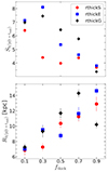 |
Fig. 5. Strength of b/p, Sb/p (top panel), and extent of b/p, Rb/p (bottom panel), calculated using thin+thick disc particles, at t = 9 Gyr shown as a function of thick-to-total mass fraction (fthick) and for different geometric configurations. With increasing fthick value, the b/ps progressively become weaker and larger in extent, and this trend remains true for all three geometric configurations considered here. The errors are calculated by constructing a total of 5000 realisations by resampling the entire population via a bootstrapping technique (for details, see text). |
3.1.2. Quantifying the b/p length and its temporal evolution
The extent of the b/p structure is another quantity of interest, and it is worth studying whether the b/p extent varies across different disc configurations and fthick values. At time t, we define the extent of the b/p structure, Rb/p, as the radial location where the peak in  profile occurs. In Lütticke et al. (2000) and Saha & Gerhard (2013), a method based on the line-of-sight surface-density profile has been formulated to quantify the size of a b/p structure. In Appendix B, we compare this method with Rb/p for the thin+thick model rthickE0.5. In Fig. 6, we show the temporal evolution of Rb/p for the thin+thick model rthickE0.5. The errors on the b/p length are estimated using the same bootstrapping technique mentioned in Sect. 3.1.1. The b/p length increases significantly (by a factor of ∼2) over the entire evolutionary phase. In addition, towards the end of the simulation run, the thick disc b/p is larger (by ∼10 − 15%) than the thin disc b/p. We found a similar trend in temporal variation of the b/p extent for other thin+thick models, and therefore they are not shown here.
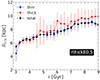 |
Fig. 6. Temporal variation of b/p extent, Rb/p, calculated using thin-, thick-disc, and thin+thick disc particles for model rthickE0.5. The b/p extent increases by a factor of ∼2 over the total simulation runtime. At t = 9 Gyr, the thick-disc b/p remains a bit larger than the thin disc b/p. The errors on Rb/p are estimated by constructing a total of 5000 realisations by resampling the entire population via a bootstrapping technique (for details, see text). |
We further checked how the extent of the b/p structure, by the end of the simulation run, varied with the thin-to-thick disc mass fraction (fthick). In Fig. 5 (bottom panel), we show the corresponding extents of the b/p structure computed at t = 9 Gyr using the thin+thick stellar particles for all thin+thick models considered here. The extent of the b/p structure increases steadily as the fthick value increases, and this trend holds true for all three different configurations considered here. Furthermore, at a fixed fthick value, the rthickG models show a higher value for the Rb/p when compared to other two configurations, thereby denoting that rthickG models form a larger b/p structure, by the end of the simulation run, as compared to rthickE and rthickS models. Lastly, in Appendix C, we show how the extent of the thin disc b/p and thick disc b/p, at the end of the simulation (t = 9 Gyr), vary across different fthick values and different disc configurations.
3.2. Vertical asymmetry and buckling instability
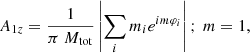
To quantify the vertical asymmetry and the time at which it occurs, we first calculated the amplitude of the first coefficient in the Fourier decomposition (A1z), which provides a measure of the asymmetry (e.g. see Martinez-Valpuesta et al. 2006; Martinez-Valpuesta & Athanassoula 2008; Saha et al. 2013). The first Fourier coefficient (A1z) is defined as (Martinez-Valpuesta & Athanassoula 2008)
 (2)
(2)
where mi is the mass of the ith particle, and φi is the angle of ith particle measured in the (x, z)-plane with the bar placed along the x-axis (side-on configuration). Mtot is denotes the total mass of the particles considered in this summation. Following Martinez-Valpuesta & Athanassoula (2008), to make this coefficient more sensitive to a buckling, we only included the stars (see Eq. (2)) that are momentarily within the extent of the b/p (Rb/p) in the summation. The corresponding temporal evolution of the buckling amplitude (A1z), calculated separately for thin, thick, and thin+thick particles, for the model rthickE0.5 is shown in Fig. 7 (left panel). A prominent peak in the A1z profile denotes the vertical buckling event. We further checked that for all the thin+thick models, a peak in the A1z is associated with the dip/decrease in the bar strength. This is expected since it is well known that the bar strength decreases as it goes through the buckling phase. The A1z amplitude is larger for the thin-disc stars when compared with that of the thick-disc stars. This is consistent is with the scenario that the thin disc b/p is stronger than the thick disc b/p.
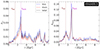 |
Fig. 7. Quantifying the vertical asymmetry in thin+thick models. Left panel: temporal evolution of A1, z (Eq. (2)) denoting vertical asymmetry in bar region, calculated using thin-disc (blue lines), thick-disc (red lines), and thin+thick disc (black lines) for the model rthickE0.5. Right panel: temporal evolution of buckling amplitude, Abuck (Eq. (3)), calculated using thin-disc (blue lines), thick-disc (red lines), and thin+thick disc (black lines) for the model rthickE0.5. The vertical magenta dotted line denotes the onset of buckling instability (τbuck), calculated from the peak of Abuck profile (for details, see text). Furthermore, for reference, we indicate the onset of bar formation (τbar, vertical maroon dotted line), calculated from the amplitude of the m = 2 Fourier moment. |
Another way of quantifying the buckling instability is by measuring the buckling amplitude, Abuck, which is defined as (for details, see Sellwood & Athanassoula 1986; Debattista et al. 2006, 2020)
 (3)
(3)
where mj, zj, and ϕj denote the mass, vertical position, and azimuthal angle of the jth particle, respectively, and the summation runs over all star particles (thin, thick, thin+thick – whichever is applicable) within the b/p extent. The quantity Abuck denotes the m = 2 vertical bending amplitude (for further details, see Debattista et al. 2006, 2020). The corresponding temporal evolution of the buckling amplitude (Abuck), calculated separately for thin, thick, and thin+thick particles for the model rthickE0.5 is shown in Fig. 7 (right panel). A prominent peak in the Abuck profile denotes the onset of the vertical buckling instability. Furthermore, the peak of value of Abuck is higher for the thin-disc than that for the thick-disc. This is again consistent with the thin disc b/p being stronger than the thick disc b/p. This trend holds true for all the thin+thick models considered here. Next, we define τbuck as the epoch for the onset of the buckling event when the peak in Abuck occurs. As seen from Fig. 7, the epoch at which the peak in A1z occurs coincides with τbuck. This is not surprising as both the quantities denote the same physical phenomenon of vertical buckling instability. In Sect. 3.3, we further investigate the variation of τbuck with fthick and its connection with bar-formation epoch.
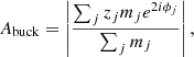
While Fig. 7 clearly demonstrates the temporal evolution of the vertical asymmetry associated with the b/p structure formation, it should be borne in mind that A1z (quantifying vertical asymmetry) or Abuck (quantifying the m = 2 vertical bending amplitude) only informs us about the buckling instability in an average sense, and hence it lacks any information about the 2D distribution of the vertical asymmetry. To investigate that, we computed the 2D distribution of the mid-plane asymmetry. Following Cuomo et al. (2023), we define
 (4)
(4)
where Σ(x, z) denotes the projected surface number density of the particles at each position of the image of the edge-on view of the model. The resulting distribution of AΣ(x, z), computed separately for the thin-disc, thick-disc, and thin+thick discs at six different times (before and after the buckling happens) are shown in Fig. 8 for the model rthickE0.5. At the initial rapid bar growth phase (t ∼ 1 Gyr), the AΣ(x, z) values remain close to zero, indicating no breaking of vertical symmetry in that evolutionary phase of the model. Around t ∼ 2.7 Gyr, the model undergoes a strong buckling event (see the peak in Fig. 7). As a result, the distribution AΣ(x, z) shows large positive and negative values at t = 2.75 Gyr, thereby demonstrating that the vertical symmetry is broken around the mid-plane. At a later time (t = 5 Gyr), the vertical symmetry is restored in the inner region (as indicated by AΣ(x, z)∼0). However, in the outer region (close to the ansae or handle of the bar), AΣ(x, z) still displays non-zero values, thereby indicating that the vertical asymmetry still persists in the outer region. Around t ∼ 6.85 Gyr, the model undergoes a second buckling event (see the second peak in A1z, albeit with smaller values in Fig. 7). As a result, at a later time (t = 6.95 Gyr), the model still shows non-zero values for AΣ(x, z) in the outer region. By the end of the simulation run (t = 9 Gyr), the values of AΣ(x, z) become close to zero throughout the entire region, thereby demonstrating that the vertical symmetry is finally restored. As Fig. 8 clearly reveals that the thin-disc stars show a larger degree of vertical asymmetry (or equivalently larger values of AΣ(x, z)) when compared with the thick-disc stars, we further checked the distribution of AΣ(x, z) in the (x, z)-plane at different times for other thin+thick models that host a prominent b/p structure. We found an overall similar trend of spatio-temporal evolution of the AΣ(x, z) as seen for the model rthickE0.5.
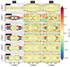 |
Fig. 8. Distribution of mid-plane asymmetry, AΣ(x, z), in the edge-on projection (x − z-plane), computed separately for the thin (left columns) and thick (middle columns) discs, as well as thin+thick (right columns) disc particles using Eq. (4) at six different times (before and after the buckling event) for the model rthickE0.5. The bar is placed along the x-axis (side-on configuration) for each time-step. Black lines denote contours of constant density. A mid-plane asymmetry persists, even long after the model has gone through the buckling phase. |
3.3. Correlation between bar and b/p properties
Past theoretical studies of the b/p formation and its subsequent growth have revealed a strong correlation between the (maximum) bar strength and the resulting (maximum) b/p strength (e.g. see Martinez-Valpuesta & Athanassoula 2008). We tested this correlation for the suite of thin+thick models considered here. The maximum bar strengths for the models are obtained from Ghosh et al. (2023) where we studied, in detail, the bar properties for these models. The maximum b/p strengths for the models are obtained from Eq. (1). We mention that all stellar particles (thin+thick) are used to calculate the maximum bar and b/p strengths for all models. The resulting distribution of the thin+thick models in maximum bar-maximum b/p strengths are shown in Fig. 9. As is seen clearly from Fig. 9, a stronger bar in a model produces a stronger b/p structure. This correlation holds true for all three geometric configurations considered here. Therefore, we also find a strong correlation between the (maximum) bar strength and the resulting (maximum) b/p strength in our thin+thick models, in agreement with past findings. In addition, we investigated the correlation (if any) between the lengths of the bar and the b/p in our thin+thick models. In Fig. 10 (top panel), we show the temporal evolution of the ratio of the b/p length (Rb/p) and the bar length (Rbar) for the model rthickE0.5. The bar length, Rbar, is defined as the radial location where the amplitude of the m = 2 Fourier moment (A2/A0) drops to 70% of its peak value (for a detailed discussion, see recent work by Ghosh & Di Matteo 2024). As is clearly seen, the ratio increases shortly after the formation of b/p, and the ratio almost saturates by the end of the simulation run (9 Gyr). Furthermore, we calculated the b/p length (Rb/p) and the bar length (Rbar), at the end of the simulation (9 Gyr) for all thin+thick models considered here. This is shown in Fig. 10 (bottom panel). For the rthickE and rthickG models, the ratio increases progressively with increasing fthick values. However, for the rthickS model, the ratio increases monotonically until fthick = 0.7, and then it starts to decrease.
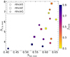 |
Fig. 9. Bar-b/p strength correlation: distribution of all thin+thick models in maximum bar strength – maximum b/p strength plane. The maximum bar strengths are taken from Ghosh et al. (2023), whereas the maximum b/p strengths are determined from Eq. (1). The colour bar denotes the thick-disc mass fraction (fthick). Different symbols represent models with different geometric configurations (see the legend). The maximum strength of the bar correlates overall with the maximum b/p strength, and this remains true for all three geometric configurations. |
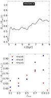 |
Fig. 10. Variation of b/p extent with varying thick-disc mass fraction. Top panel: temporal evolution of ratio of b/p length (Rb/p) and bar length (Rbar) for model rthickE0.5. Bottom panel: variation of ratio of b/p and bar length, calculated at the end of the simulation run (t = 9 Gyr), with thick-disc mass fraction (fthick). |
Lastly, we investigated the time delay between the bar formation and the onset of buckling instability for all thin+thin models considered here, and we studied if and how it varies with thick-disc mass fraction (fthick). In Appendix D, we show how the bar-formation epoch, τbar, varies with different fthick values and with different disc configurations. Similarly, in Sect. 3.2, we define the epoch of buckling instability when the peak in Abuck occurs. The resulting variation of the time delay, τbuck − τbar with fthick is shown in Fig. 11. For a fixed geometric configuration (rthickE, rthickS, or rthickG), the time interval between the bar formation and the onset of buckling instability becomes progressively shorter with increasing fthick values. This happens due to the fact that with increasing fthick, the bar forms progressively at a later stage (see Appendix D). In addition, for a fixed fthick value, the rthickS models almost always show shorter time delay (τbuck − τbar) when compared to other two geometric configurations considered here (see Fig. 11).
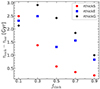 |
Fig. 11. Variation of time delay between the formation and onset of buckling instability, τbuck − τbar, with thick-disc mass fraction (fthick), for all thin+thick models considered here. For a fixed geometric configuration, τbuck − τbar becomes progressively shorter with increasing fthick values (for details, see text). |
4. Kinematic signatures of buckling and its connection with b/p formation
Understanding the temporal evolution of the diagonal and off-diagonal components of the stellar velocity tensor was shown to be instrumental for investigating the formation and growth of the b/p structure (see Saha et al. 2013, and references therein). Here, we systematically studied some key diagonal and off-diagonal components of the stellar velocity dispersion tensor and their associated temporal evolution for all the thin+thick models considered.
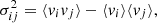
At a given radius R, the stellar velocity dispersion tensor is defined as (Binney & Tremaine 2008)
 (5)
(5)
where quantities within the ⟨⟩ brackets denote the average quantities, and the averaging is done for a group of stars. Here, i, j = R, ϕ, z. The corresponding stress tensor of the stellar fluid is defined as
 (6)
(6)
where ρ(R) denotes the local volume density of stars at a radial location R. τn and τs denote the normal stress (acting along the normal to a small differential imaginary surface dS) and the shear stress (acting along the perpendicular to the normal to dS), respectively (for further details, see Binney & Tremaine 2008; Saha et al. 2013). The components of τn are determined by the diagonal elements of the velocity dispersion tensor, while the shear stress is determined by the off-diagonal elements of the velocity dispersion tensor (for details, see Binney & Tremaine 2008). Furthermore, the diagonal elements of the velocity dispersion tensor determines the axial ratios of the stellar velocity ellipsoid with respect to the galactocentric axes  , whereas the orientations of the velocity ellipsoid are determined by the off-diagonal elements of the velocity dispersion tensor (for details, see Binney & Tremaine 2008; Saha et al. 2013). One such quantity of interest is the meridional tilt angle, which is defined as
 (7)
(7)
The tilt angle, Θtilt, denotes the orientation or the deformation of the stellar velocity ellipsoid in the meridional plane (R − z-plane). In the past, it was shown for an N-body model that when the bar grows, it causes much radial heating (or equivalently, increasing the radial velocity dispersion, σRR) without causing a similar degree of heating the vertical direction (or equivalently, no appreciable increase in the vertical velocity dispersion, σzz). Consequently, the model goes through a vertical buckling instability causing the thickening of the inner part, which in turn also increases σzz (e.g. Debattista et al. 2004; Martinez-Valpuesta et al. 2006; Martinez-Valpuesta & Athanassoula 2008; Saha et al. 2013; Fragkoudi et al. 2017b; Di Matteo et al. 2019). Therefore, it is of great interest to investigate the temporal evolution of the vertical-to-radial velocity dispersion (σzz/σRR) in order to fully grasp the formation and growth of b/p structure in our thin+thick models. In addition, using N-body simulations, Saha et al. (2013) demonstrated that during the onset of the buckling phase, the model shows a characteristic increase in the meridional tilt angle, Θtilt, which in turn could be used as an excellent diagnostic to identify an ongoing buckling phase in real observed galaxies. In this work, we studied the temporal evolution of these dynamical quantities in detail for all the thin+thick models considered.
In Appendix E, we show the radial profiles of vertical-to-radial velocity dispersion as a function of time for the model rthickE0.5. In order to quantify the temporal evolution of σzz/σRR, we computed them using Eq. (5) within the extent of the b/p structure (Rb/p). The corresponding temporal evolution of the vertical-to-radial velocity dispersion (σzz/σRR), calculated separately for thin, thick, and thin+thick particles, is shown in Fig. 12 (left panel) for the model rthickE0.5. As seen from Fig. 12, the temporal evolution of σzz/σRR displays a characteristic U shape (of different amplitudes) during the course of the evolution, arising from the radial heating of the bar (increase in σRR) and the subsequent vertical thickening (increase in σzz) due to the buckling instability. In addition, the temporal profiles of σzz/σRR for the thin disc show a larger and more prominent U-shaped feature when compared with that for the thick-disc stars. This is consistent with the notion that thin-disc b/p are, in general, stronger than the thick-disc b/p. The epoch corresponding to the maximum increase in the quantity σzz/σRR coincides with the peak in the Abuck, denoting strong vertical buckling instability (see the location of vertical magenta line in Fig. 12). This further demonstrates that the b/p structures in our thin+thick models are indeed formed through vertical buckling instability. In Appendix E, we show the temporal evolution of σzz/σRR for all thin+thick models considered here. We checked the trends mentioned above hold true for all the models that formed a b/p structure during the evolutionary trajectory.
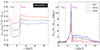 |
Fig. 12. Quantifying the kinematic signature of teh vertical buckling instability and the subsequent b/p formation. Left panel: temporal evolution of vertical-to-radial velocity dispersion (σzz/σRR), calculated within the b/p extent (Rb/p), (σzz/σRR)2(t; R ≤ Rb/p), for thin (in blue), thick (in red), and total (thin+thick) disc (in black) particles, for model rthickE0.5. Right panel: temporal evolution of meridional tilt angle (Θtilt), calculated within Rb/p using Eq. (7), for thin (in blue), thick (in red), and total (thin+thick) disc (in black) particles, for model rthickE0.5. The vertical maroon dotted line denotes the onset of bar formation (τbar), while the vertical magenta dotted line denotes the onset of buckling instability (τbuck; for details, see text). |
Lastly, we investigated the temporal evolution of the meridional tilt angle, Θtilt for the model rthickE0.5. Figure 12 (right panel) shows the corresponding temporal evolution of the tilt angle, Θtilt, calculated separately for thin, thick, and thin+thick particles using Eq. (7) for the model rthickE0.5. The temporal evolution of Θtilt shows a characteristic increase during the course of evolution. The epoch of the maximum value of the tilt angle coincides with the epoch of strong buckling instability (see the location of vertical magenta line in Fig. 12). This is in agreement with the findings of Saha et al. (2013) and is consistent with a “b/p formed through buckling” scenario. Furthermore, the temporal profiles of Θtilt for the thin disc shows a larger and more prominent peak when compared with that for the thick-disc stars. This is expected as the thin-disc b/p is stronger than the thick-disc b/p. We checked that the trends, mentioned above, hold true for all the models that formed a b/p structure during the evolutionary trajectory. For the sake of brevity, they are not shown here.
5. X-shape of the b/p and relative contribution of thin disc
A visual inspection of Fig. 1 already revealed that for a fixed geometric configuration, the appearance of the b/p structure changes from more X-shaped to more boxy as the thick-disc mass fraction steadily increases. This trend is more prominent for the rthickE and rthickG models (see middle and right panels of Fig. 1). Here, we investigate this in further detail. In addition, we also investigate how the thin- and thick-disc stars contribute to the formation of the b/p structure.
To carry out the detailed analysis, we first chose two models, namely, rthickE0.1 and rthickE0.9. In the rthickE0.1 model, the thin-disc stars dominate the underlying mass distribution, whereas in the rthickE0.9 model, the thick-disc stars dominate the mass distribution, thereby providing an ideal scenario for the aforementioned investigation. In Fig. 13 (top left panels), we show the density contours of the edge-on stellar (thin+thick) distribution (with bar placed along the x-axis) in the central region encompassing the b/p structure. This clearly brings out the stark differences in the morphology of density contours. In the rthickE0.1 model, the contours have a more prominent X-shaped appearance, whereas in the rthickE0.9 model, the contours have a more prominent box-shaped appearance. Figure 13 (bottom left panels) shows the density profiles along the bar major axis, calculated at different heights (from the mid-plane) for these two thin+thick models. At larger heights, a bimodality in the density profiles along the bar major axis reconfirms the strong X-shaped feature for the rthickE0.1 model. For the rthickE0.9 model, no such bimodality in the density profiles along the bar major axis is seen, thereby confirming that the b/p structure is more box-shaped in the rthickE0.9 model. Furthermore, we calculated the vertical stellar density distribution at a radial location around the peak of the b/p structure (see vertical blue lines in top left panels of Fig. 13) for these two models. A careful inspection reveals that the vertical stellar density distribution for the rthickE0.1 model is more centrally peaked (with well-defined tails), whereas vertical stellar density distribution for the rthickE0.9 model is broader, especially at larger heights (see right panel of Fig. 13).
 |
Fig. 13. Variation of the b/p morphology with varying thick-disc mass faction (fthick). Top left panels: density contours of edge-on stellar (thin+thick) distribution (with bar placed along the x-axis) in central region at t = 9 Gyr for models rthickE0.1 and rthickE0.9. For the rthickE0.1 model, the contours display more prominent X-shaped feature, whereas for the rthickE0.9 model, the contours display more prominent box-shaped feature. Bottom left panels: density profiles (normalised by the peak density value, and in log-scale) along bar major axis, calculated at different heights (from |z| = 0 to 6 kpc, with a step-size of 1 kpc) from mid-plane, for models rthickE0.1 and rthickE0.9. The density profiles have been artificially shifted along the y-axis to show the trends as height changes, and they do not overlap. Right panel: vertical stellar density distribution (normalised by the peak density value, and in log-scale), at a radial location around peak of the b/p structure (marked by blue vertical lines in top left panels) for rthickE0.1 and rthickE0.9 models. |
To further investigate how the thin- and thick-disc stars contribute to the formation of the b/p structure, we calculated the thin-disc mass fraction, fthin(=1 − fthick) at the end of the simulation run (t = 9 Gyr). Figure 14 shows the corresponding distribution of the thin-disc mass fraction in the edge-on projection (x − z-plane) for all thin+thick disc models. In each case, the bar is placed in side-on configuration (along the x-axis). As is seen clearly from Fig. 14, the thin-disc stars dominate in central regions close to the mid-plane (z = 0) and are responsible for giving rise to a strong X-shape of the b/p structure, in agreement with the findings of past studies (see e.g. Di Matteo 2016; Athanassoula et al. 2017; Debattista et al. 2017; Fragkoudi et al. 2017b, 2020). As one moves farther away from the mid-plane, the thick-disc stars start to dominate progressively. Furthermore, the appearance of the b/p structure changes from more X-shaped to more box-shaped as the thick-disc mass fraction steadily increases. These trends remain generic for all three geometric configurations (different thin-to-thick disc scale length ratios) considered here.
 |
Fig. 14. Fraction of thin-disc stars, fthin(=1 − fthick), in the edge-on projection (with the bar placed along the x-axis) compared to the total (thin+thick) disc, at the end of the simulation run (t = 9 Gyr) for all thin+thick disc models with varying fthick values. Left panels show the distribution for the rthickS models, whereas middle panels and right panels show the distribution for the rthickE and rthickG models, respectively. The values of (fthick) vary from 0.1 to 0.9 (top to bottom), as indicated in the left-most panel of each row. For each model, the fraction of thin-disc stars decreases with height from the mid-plane (z = 0). In addition, the appearance of the b/p structure changes from more X-shaped to more boxy-shaped as the thick-disc mass fraction steadily increases. |
6. Discussion
In what follows, we discuss some of the implications and limitations of this work. First, our findings demonstrate that the b/p structure can form even in the presence of a massive thick-disc component. This provides a natural explanation to the presence of b/p in high-redshift (z = 1) disc galaxies in the hypothesis that these high-z discs have a significant fraction of their mass in a thick disc (see e.g. Hamilton-Campos et al. 2023). A recent work by Kruk et al. (2019) estimated that at z ∼ 1, about 10% of barred galaxies would harbour a b/p. Therefore, our results are in agreement with the recent observational trends. In addition, bars forming in the presence of a massive thick disc (as shown in a recent work of Ghosh et al. 2023) and the present work showing that b/ps also form in the presence of a massive thick disc suggest that bar and b/p bulge formation may have appeared at earlier redshifts than what has been considered so far, as well as in galaxies dominated by a thick-disc component. The findings that the b/p morphology and length depend on the thick-disc fraction (the higher the thick-to-thin disc mass ratio, the more boxy the corresponding b/p and the smaller its extent) may be taken as a prediction that can be tested in current and future observations (the JWST, for example).
Secondly, the occurrence of b/p in disc galaxies is observationally found to be strongly dependent on the stellar mass of the galaxy in the local Universe (Yoshino & Yamauchi 2015; Erwin & Debattista 2017; Marchuk et al. 2022) as well as at higher redshifts (Kruk et al. 2019). This implies that a galaxy’s stellar mass is likely to play an important role in forming b/ps via vertical instabilities. In our suite of thin+thick models, although we systematically varied the thick-disc mass fraction, the total stellar mass remained fixed (∼1 × 10¹¹ M⊙). Investigating the role of the stellar mass on b/p formation via vertical buckling instability would be quite interesting; however, it is beyond the scope of the present work.
Furthermore, in our thin+thick models, the stars are separated into two well-defined and distinct populations, namely, thin- and thick-disc stars. While this might be well-suited for external galaxies, this scheme is a simplification for the Milky Way. Bovy et al. (2012) showed that the disc properties vary continuously with the scale height in the Milky Way. Nevertheless, our adapted scheme of discretising stars with a varying fraction of thick-disc stars provides valuable insight into the trends, as it has been shown for the MW that a two-component disc can already capture the main trends found in more complex, multi-component discs (e.g. see Di Matteo 2016; Debattista et al. 2017; Fragkoudi et al. 2017b, 2018a,b, 2020).
Finally, if these b/p structures also formed at high redshift, two additional questions arise. These concern the role of interstellar gas, which is particularly critical in high-z discs that are gas-rich, and the role of mergers and accretions, which high-z galaxies may have experienced at high rates – in maintaining/perturbing/destroying bars and b/p bulges. The role of the interstellar gas in the context of the generation/destruction of disc instabilities, such as bars (Bournaud et al. 2005) and spiral arms (Sellwood & Carlberg 1984; Ghosh & Jog 2015, 2016, 2022), has been investigated in past literature. In addition, the b/p bulges play a key role in evolution of disc galaxies by regulating the bar-driven gas inflow (e.g. see Fragkoudi et al. 2015, 2016). Furthermore, bars can be weakened substantially (or even destroyed in some cases) as a result of minor mergers (Ghosh et al. 2021). Therefore, it would be worth investigating the b/p formation and evolution scenario in the presence of the thick disc and the interstellar gas and how likely they are to be affected by the merger events.
7. Summary
In summary, we investigated the dynamical role of a geometrically thick disc on the b/p formation and their subsequent evolution scenario. We made use of a suite of N-body models of thin+thick discs and systematically varied mass fractions of the thick disc and the different thin-to-thick disc scale length ratios. Our main findings are listed below.
-
B/ps form in almost all thin+thick disc models with varying thick-disc mass fractions and for all three geometric configurations with different thin-to-thick disc scale length ratios. The thick-disc b/p always remains weaker than the thin-disc b/p, and this remains valid for all three geometric configurations considered here.
-
The final b/p strength shows an overall decreasing trend with increasing thick-disc mass fraction (fthick). In addition, the b/ps in simulated galaxies with shorter thick-disc scale lengths form at earlier times and show a rapid initial growth phase when compared to the other two geometric configurations. Furthermore, we found a strong (positive) correlation between the maximum bar and b/p strengths in our thin+thick models.
-
For a fixed geometric configuration, the time interval between the bar formation and the onset of vertical buckling instability becomes progressively shorter with an increasing thick-disc mass fraction. In addition, for a fixed thick-disc mass fraction, models with shorter thick-disc scale length display shorter time delay between the bar formation and the onset of a buckling event when compared to the other two geometric configurations.
-
The final b/p length shows an overall increasing trend with increasing thick-disc mass fraction (fthick), and this remains valid for all three geometric configurations considered here. In addition, for a fixed fthick value, the models with larger thick-disc scale lengths form a larger b/p structure when compared to the other two geometric configurations. Furthermore, the weaker b/ps are more extended structures (i.e. larger Rb/p).
-
The b/p structure changes appearance from being more X-shaped to being more box-shaped as the fthick values increase monotonically. This trend holds true for all three geometric configurations. Furthermore, the thin-disc stars are predominantly responsible for giving rise to a strong X-shape of the b/p structure.
-
Our thin+thick models go through a vertical buckling instability phase to form the b/p structure. The thin-disc stars display a higher degree of vertical asymmetry and buckling when compared to the thick-disc stars. Furthermore, the vertical asymmetry persists long after the buckling phase is over; the vertical symmetry in the inner region is restored relatively quickly, while the vertical symmetry in the outer region (close to the ansae or handle of the bar) is restored long after the buckling event is over.
-
The thin+thick models demonstrate characteristic signatures in the temporal evolution of different diagonal (σzz/σRR ratio) and off-diagonal (meridional tilt angle, Θtilt) components of the stellar velocity dispersion tensor, as one would expect if the b/p structure is formed via the vertical buckling instability. These kinematic signatures are more prominent when computed using only the thin-disc stars as compared to using only the thick-disc stars.
To conclude, even in the presence of a massive (kinematically hot) thick-disc component, the models are to able to harbour a prominent b/p structure formed via vertical buckling instability. This clearly implies that b/ps can form in thick discs at high redshifts and is in agreement with the observational evidence of the presence of b/ps at high redshifts (Kruk et al. 2019). Our results presented here also predict that at higher redshifts, the b/p will have a more boxy appearance than a more X-shaped one, which remains to be tested in future observations at higher redshifts (z = 1 and beyond).
Acknowledgments
S.G. acknowledges funding from the Alexander von Humboldt Foundation, through Dr. Gregory M. Green’s Sofja Kovalevskaja Award. We thank the anonymous referee for useful comments which helped to improve this paper. This work has made use of the computational resources obtained through the DARI grant A0120410154 (P.I.: P. Di Matteo).
References
- Anderson, S. R., Gough-Kelly, S., Debattista, V. P., et al. 2024, MNRAS, 527, 2919 [Google Scholar]
- Athanassoula, E. 2016, in Galactic Bulges, eds. E. Laurikainen, R. Peletier, & D. Gadotti, Astrophys. Space Sci. Lib., 418, 391 [NASA ADS] [CrossRef] [Google Scholar]
- Athanassoula, E., Rodionov, S. A., & Prantzos, N. 2017, MNRAS, 467, L46 [Google Scholar]
- Aumer, M., & Binney, J. 2017, MNRAS, 470, 2113 [NASA ADS] [CrossRef] [Google Scholar]
- Barnes, J., & Hut, P. 1986, Nature, 324, 446 [NASA ADS] [CrossRef] [Google Scholar]
- Binney, J., & Tremaine, S. 2008, Galactic Dynamics: Second Edition (Princeton: Princeton University Press) [Google Scholar]
- Bournaud, F., Combes, F., & Semelin, B. 2005, MNRAS, 364, L18 [Google Scholar]
- Bovy, J., Rix, H.-W., Liu, C., et al. 2012, ApJ, 753, 148 [Google Scholar]
- Buck, T., Ness, M., Obreja, A., Macciò, A. V., & Dutton, A. A. 2019, ApJ, 874, 67 [NASA ADS] [CrossRef] [Google Scholar]
- Bureau, M., & Freeman, K. C. 1999, AJ, 118, 126 [NASA ADS] [CrossRef] [Google Scholar]
- Burstein, D. 1979, ApJ, 234, 829 [NASA ADS] [CrossRef] [Google Scholar]
- Buta, R. 1995, ApJS, 96, 39 [Google Scholar]
- Buta, R., & Crocker, D. A. 1991, AJ, 102, 1715 [NASA ADS] [CrossRef] [Google Scholar]
- Combes, F., & Sanders, R. H. 1981, A&A, 96, 164 [NASA ADS] [Google Scholar]
- Combes, F., Debbasch, F., Friedli, D., & Pfenniger, D. 1990, A&A, 233, 82 [NASA ADS] [Google Scholar]
- Comerón, S., Knapen, J. H., Sheth, K., et al. 2011a, ApJ, 729, 18 [CrossRef] [Google Scholar]
- Comerón, S., Elmegreen, B. G., Knapen, J. H., et al. 2011b, ApJ, 741, 28 [CrossRef] [Google Scholar]
- Comerón, S., Salo, H., Peletier, R. F., & Mentz, J. 2016, A&A, 593, L6 [NASA ADS] [CrossRef] [EDP Sciences] [Google Scholar]
- Comerón, S., Salo, H., & Knapen, J. H. 2018, A&A, 610, A5 [NASA ADS] [CrossRef] [EDP Sciences] [Google Scholar]
- Comerón, S., Salo, H., Knapen, J. H., & Peletier, R. F. 2019, A&A, 623, A89 [NASA ADS] [CrossRef] [EDP Sciences] [Google Scholar]
- Cuomo, V., Debattista, V. P., Racz, S., et al. 2023, MNRAS, 518, 2300 [Google Scholar]
- Debattista, V. P., Carollo, C. M., Mayer, L., & Moore, B. 2004, ApJ, 604, L93 [NASA ADS] [CrossRef] [Google Scholar]
- Debattista, V. P., Mayer, L., Carollo, C. M., et al. 2006, ApJ, 645, 209 [Google Scholar]
- Debattista, V. P., Ness, M., Gonzalez, O. A., et al. 2017, MNRAS, 469, 1587 [Google Scholar]
- Debattista, V. P., Liddicott, D. J., Khachaturyants, T., & Beraldo e Silva, L. 2020, MNRAS, 498, 3334 [Google Scholar]
- Di Matteo, P. 2016, PASA, 33, e027 [CrossRef] [Google Scholar]
- Di Matteo, P., Haywood, M., Gómez, A., et al. 2014, A&A, 567, A122 [NASA ADS] [CrossRef] [EDP Sciences] [Google Scholar]
- Di Matteo, P., Fragkoudi, F., Khoperskov, S., et al. 2019, A&A, 628, A11 [NASA ADS] [CrossRef] [EDP Sciences] [Google Scholar]
- Elmegreen, B. G., Elmegreen, D. M., & Hirst, A. C. 2004, ApJ, 612, 191 [NASA ADS] [CrossRef] [Google Scholar]
- Erwin, P., & Debattista, V. P. 2013, MNRAS, 431, 3060 [Google Scholar]
- Erwin, P., & Debattista, V. P. 2016, ApJ, 825, L30 [NASA ADS] [CrossRef] [Google Scholar]
- Erwin, P., & Debattista, V. P. 2017, MNRAS, 468, 2058 [Google Scholar]
- Fragkoudi, F., Athanassoula, E., Bosma, A., & Iannuzzi, F. 2015, MNRAS, 450, 229 [NASA ADS] [CrossRef] [Google Scholar]
- Fragkoudi, F., Athanassoula, E., & Bosma, A. 2016, MNRAS, 462, L41 [NASA ADS] [CrossRef] [Google Scholar]
- Fragkoudi, F., Di Matteo, P., Haywood, M., et al. 2017a, A&A, 607, L4 [NASA ADS] [CrossRef] [EDP Sciences] [Google Scholar]
- Fragkoudi, F., Di Matteo, P., Haywood, M., et al. 2017b, A&A, 606, A47 [NASA ADS] [CrossRef] [EDP Sciences] [Google Scholar]
- Fragkoudi, F., Di Matteo, P., Haywood, M., et al. 2018a, in Rediscovering Our Galaxy, eds. C. Chiappini, I. Minchev, E. Starkenburg, & M. Valentini, 334, 288 [NASA ADS] [Google Scholar]
- Fragkoudi, F., Di Matteo, P., Haywood, M., et al. 2018b, A&A, 616, A180 [NASA ADS] [CrossRef] [EDP Sciences] [Google Scholar]
- Fragkoudi, F., Grand, R. J. J., Pakmor, R., et al. 2020, MNRAS, 494, 5936 [Google Scholar]
- Ghosh, S., & Di Matteo, P. 2024, A&A, 683, A100 [NASA ADS] [CrossRef] [EDP Sciences] [Google Scholar]
- Ghosh, S., & Jog, C. J. 2015, MNRAS, 451, 1350 [NASA ADS] [CrossRef] [Google Scholar]
- Ghosh, S., & Jog, C. J. 2016, MNRAS, 459, 4057 [NASA ADS] [CrossRef] [Google Scholar]
- Ghosh, S., & Jog, C. J. 2018, A&A, 617, A47 [NASA ADS] [CrossRef] [EDP Sciences] [Google Scholar]
- Ghosh, S., & Jog, C. J. 2022, A&A, 658, A171 [NASA ADS] [CrossRef] [EDP Sciences] [Google Scholar]
- Ghosh, S., Saha, K., Di Matteo, P., & Combes, F. 2021, MNRAS, 502, 3085 [NASA ADS] [CrossRef] [Google Scholar]
- Ghosh, S., Fragkoudi, F., Di Matteo, P., & Saha, K. 2023, A&A, 674, A128 [NASA ADS] [CrossRef] [EDP Sciences] [Google Scholar]
- Guo, Y., Jogee, S., Finkelstein, S. L., et al. 2023, ApJ, 945, L10 [NASA ADS] [CrossRef] [Google Scholar]
- Hamilton-Campos, K. A., Simons, R. C., Peeples, M. S., Snyder, G. F., & Heckman, T. M. 2023, ApJ, 956, 147 [NASA ADS] [CrossRef] [Google Scholar]
- Jogee, S., Barazza, F. D., Rix, H.-W., et al. 2004, ApJ, 615, L105 [NASA ADS] [CrossRef] [Google Scholar]
- Kasparova, A. V., Katkov, I. Y., Chilingarian, I. V., et al. 2016, MNRAS, 460, L89 [NASA ADS] [CrossRef] [Google Scholar]
- Klypin, A., Valenzuela, O., Colín, P., & Quinn, T. 2009, MNRAS, 398, 1027 [Google Scholar]
- Kruk, S. J., Erwin, P., Debattista, V. P., & Lintott, C. 2019, MNRAS, 490, 4721 [Google Scholar]
- Laurikainen, E., Salo, H., Buta, R., & Knapen, J. H. 2011, MNRAS, 418, 1452 [Google Scholar]
- Le Conte, Z. A., Gadotti, D. A., Ferreira, L., et al. 2023, MNRAS, submitted [arXiv:2309.10038] [Google Scholar]
- Li, X., Shlosman, I., Pfenniger, D., & Heller, C. 2023, MNRAS, 520, 1243 [NASA ADS] [CrossRef] [Google Scholar]
- Lütticke, R., Dettmar, R. J., & Pohlen, M. 2000, A&AS, 145, 405 [NASA ADS] [CrossRef] [EDP Sciences] [Google Scholar]
- Marchuk, A. A., Smirnov, A. A., Sotnikova, N. Y., et al. 2022, MNRAS, 512, 1371 [NASA ADS] [CrossRef] [Google Scholar]
- Martig, M., Pinna, F., Falcón-Barroso, J., et al. 2021, MNRAS, 508, 2458 [NASA ADS] [CrossRef] [Google Scholar]
- Martinez-Valpuesta, I., & Athanassoula, E. 2008, in Formation and Evolution of Galaxy Bulges, eds. M. Bureau, E. Athanassoula, & B. Barbuy, 245, 103 [NASA ADS] [Google Scholar]
- Martinez-Valpuesta, I., Shlosman, I., & Heller, C. 2006, ApJ, 637, 214 [NASA ADS] [CrossRef] [Google Scholar]
- McWilliam, A., & Zoccali, M. 2010, ApJ, 724, 1491 [NASA ADS] [CrossRef] [Google Scholar]
- Merritt, D., & Sellwood, J. A. 1994, ApJ, 425, 551 [NASA ADS] [CrossRef] [Google Scholar]
- Miyamoto, M., & Nagai, R. 1975, PASJ, 27, 533 [NASA ADS] [Google Scholar]
- Nataf, D. M., Udalski, A., Gould, A., Fouqué, P., & Stanek, K. Z. 2010, ApJ, 721, L28 [NASA ADS] [CrossRef] [Google Scholar]
- Ness, M., Freeman, K., Athanassoula, E., et al. 2012, ApJ, 756, 22 [NASA ADS] [CrossRef] [Google Scholar]
- Pérez, I., Martínez-Valpuesta, I., Ruiz-Lara, T., et al. 2017, MNRAS, 470, L122 [CrossRef] [Google Scholar]
- Pinna, F., Falcón-Barroso, J., Martig, M., et al. 2019a, A&A, 625, A95 [NASA ADS] [CrossRef] [EDP Sciences] [Google Scholar]
- Pinna, F., Falcón-Barroso, J., Martig, M., et al. 2019b, A&A, 623, A19 [NASA ADS] [CrossRef] [EDP Sciences] [Google Scholar]
- Plummer, H. C. 1911, MNRAS, 71, 460 [Google Scholar]
- Pohlen, M., Balcells, M., Lütticke, R., & Dettmar, R. J. 2004, A&A, 422, 465 [NASA ADS] [CrossRef] [EDP Sciences] [Google Scholar]
- Press, W. H., Flannery, B. P., & Teukolsky, S. A. 1986, Numerical Recipes. The Art of Scientific Computing (Cambridge: Cambridge University Press) [Google Scholar]
- Quillen, A. C. 2002, AJ, 124, 722 [NASA ADS] [CrossRef] [Google Scholar]
- Quillen, A. C., Kuchinski, L. E., Frogel, J. A., & DePoy, D. L. 1997, ApJ, 481, 179 [NASA ADS] [CrossRef] [Google Scholar]
- Quillen, A. C., Minchev, I., Sharma, S., Qin, Y.-J., & Di Matteo, P. 2014, MNRAS, 437, 1284 [Google Scholar]
- Raha, N., Sellwood, J. A., James, R. A., & Kahn, F. D. 1991, Nature, 352, 411 [Google Scholar]
- Rodionov, S. A., Athanassoula, E., & Sotnikova, N. Y. 2009, MNRAS, 392, 904 [NASA ADS] [CrossRef] [Google Scholar]
- Saha, K., & Gerhard, O. 2013, MNRAS, 430, 2039 [NASA ADS] [CrossRef] [Google Scholar]
- Saha, K., Pfenniger, D., & Taam, R. E. 2013, ApJ, 764, 123 [NASA ADS] [CrossRef] [Google Scholar]
- Saha, K., Graham, A. W., & Rodríguez-Herranz, I. 2018, ApJ, 852, 133 [NASA ADS] [CrossRef] [Google Scholar]
- Scott, N., van de Sande, J., Sharma, S., et al. 2021, ApJ, 913, L11 [NASA ADS] [CrossRef] [Google Scholar]
- Sellwood, J. A., & Athanassoula, E. 1986, MNRAS, 221, 195 [NASA ADS] [Google Scholar]
- Sellwood, J. A., & Carlberg, R. G. 1984, ApJ, 282, 61 [Google Scholar]
- Sellwood, J. A., & Gerhard, O. 2020, MNRAS, 495, 3175 [Google Scholar]
- Semelin, B., & Combes, F. 2002, A&A, 388, 826 [NASA ADS] [CrossRef] [EDP Sciences] [Google Scholar]
- Shen, J., Rich, R. M., Kormendy, J., et al. 2010, ApJ, 720, L72 [NASA ADS] [CrossRef] [Google Scholar]
- Sheth, K., Elmegreen, D. M., Elmegreen, B. G., et al. 2008, ApJ, 675, 1141 [Google Scholar]
- Tsikoudi, V. 1979, ApJ, 234, 842 [NASA ADS] [CrossRef] [Google Scholar]
- Vynatheya, P., Saha, K., & Ghosh, S. 2021, MNRAS, submitted [arXiv:2105.03183] [Google Scholar]
- Wegg, C., & Gerhard, O. 2013, MNRAS, 435, 1874 [Google Scholar]
- Wegg, C., Gerhard, O., & Portail, M. 2015, MNRAS, 450, 4050 [NASA ADS] [CrossRef] [Google Scholar]
- Yoachim, P., & Dalcanton, J. J. 2006, AJ, 131, 226 [NASA ADS] [CrossRef] [Google Scholar]
- Yoshino, A., & Yamauchi, C. 2015, MNRAS, 446, 3749 [Google Scholar]
Appendix A: B/p strength from the Fourier decomposition
Following Martinez-Valpuesta et al. (2006) and Martinez-Valpuesta & Athanassoula (2008), at time t, we define the strength of the b/p as
![Mathematical equation: $$ \begin{aligned} C_{m, z} = \left|\sum _{i=1} ^{N_s} z_i \exp [{i m z_i/(5 \langle {z_{\rm d}}\rangle )}] \right|; m =2, \end{aligned} $$](/articles/aa/full_html/2024/03/aa47831-23/aa47831-23-eq24.gif) (A.1)
(A.1)
where zi denotes the vertical position of the ith particle, and Ns denotes the total number of stellar particles (thin+thick) within the extent of the b/p. ⟨zd⟩ denotes the average scale height of the total disc and is calculated in the following way:
 (A.2)
(A.2)
In Fig. A.1, we show the temporal evolution of C2, z, computed using Eq. A.1 for the model rthickE0.5 and compare the corresponding b/p strength calculated using Eq. 1. As seen clearly from Fig. A.1, there is a one-to-one correspondence between the b/p strengths, calculated using Eq. A.1 and Eq. 1. We checked this for other thin+thick models as well and found a similar trend to that seen for the model rthickE0.5. For the sake of brevity, they are not shown here.
 |
Fig. A.1. Temporal evolution of C2, z, b/p strength computed from the Fourier decomposition using Eq. A.1, plotted against the b/p strength calculated using Eq. 1 for the model rthickE0.5. All the stellar particles (thin+thick) within the b/p extent (Rb/p) are used in both cases. The colour bar denotes the time of the simulation. Both the measures of b/p strength correlate fairly well. |
Appendix B: B/p length from the LOS surface-density profile
Lütticke et al. (2000) and Saha & Gerhard (2013) measured the size of the b/p structure, Lb/p, by finding zeros of the function Dg(x, z) defined by
 (B.1)
(B.1)
for a set of smoothed surface-density (Σlos) profiles while placing the bar along the x-axis. In Fig. B.1 (top panel), we show the profiles of the function Dg(x, z) at three different times where the Σlos(x, z) profiles are calculated at z = 0.8Rd, thin (for further details, see Saha & Gerhard 2013). Fig. B.1 (bottom panel) shows the correlation of b/p size, Lb/p (computed by finding zeros of function Dg(x, z)) with the b/p length, Rb/p. As seen clearly, these two quantities are strongly correlated with the Pearson correlation coefficient, ρ ∼ 0.95. However, at all times, the values of Lb/p remain larger than that of Rb/p, as also can be judged from the slope of the best-fit straight line (see black dashed line in bottom panel of Fig. B.1).
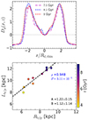 |
Fig. B.1. Comparison of different methods for measuring the b/p extent. Top panel: Profiles of function Dg(x, z) (see Eq. (B.1)), calculated at three different times for model rthickE0.5. The horizontal dotted line denotes the zeros of the function Dg(x, z) (for details, see text). Bottom panel: Correlations between size of the b/p, Lb/p and the b/p length Rb/p for the model rthickE0.5. A straight line of the form Y = AX + B is fitted (black dashed line), and the corresponding best-fit parameters are quoted. The Pearson correlation coefficients are quoted (see top right). Here, Rd, thin = 4.7 kpc. |
Appendix C: Thin- & thick-disc b/p lengths as a function of thick-disc mass fraction
Here, we briefly investigate how the extent of the thin and thick disc b/ps, at the end of the simulation run (t = 9 Gyr) vary with the thick-disc mass fraction in all three geometric configurations considered here. This is shown in Fig. C.1. For a given thin+thick model, the thin disc b/p always remains shorter than the thick disc b/p, and this holds for almost all thin+thick models considered here.
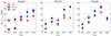 |
Fig. C.1. B/p extent, at the end of the simulation run (t = 9 Gyr), computed for the thin and thick discs, as well as for the thin+thick case, for all the thin+thick models considered here. Left panels show the distribution for the rthickS models, whereas middle panels and right panels show the distribution for the rthickE and rthickG models, respectively. Thin disc b/ps always remain shorter than the thick disc b/ps. The errors on Rb/p are estimated by constructing a total of 5,000 realisations by resampling the entire population via a bootstrapping technique (for details, see Sect. 3.1.2). |
Appendix D: Bar-formation epoch and its variation with the thick-disc mass fraction
In Ghosh et al. (2023), we showed that the bars in rthickS models tend to form earlier when compared to the other two models (rthickE and rthickG). However, the bar-formation epoch was not quantified in Ghosh et al. (2023). Here, we study this and also investigate how it varies with the thick-disc mass fraction. The bar formation epoch, τbar, is defined when the amplitude of the m = 2 Fourier moment becomes greater than 0.2 and the corresponding phase angle, ϕ2, remains constant (within 3 − 5°) within the extent of the bar. In Fig. D.1, we show the corresponding variation of the bar-formation epoch, τbar, as a function of the thick-disc mass fraction, for all three geometric configurations considered here. As seen clearly, for a fixed fthick value, bars form at an earlier epoch in rthickS models as compared to the other two configurations. In addition, for a given geometric configuration, the bar-formation epoch progressively increases with increasing fthick values.
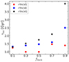 |
Fig. D.1. Variation of bar formation epoch, τbar, as a function of thick-disc mass fraction (fthick), for all thin+thick models considered here. For a given geometric configuration, the bar formation epoch increases with increasing fthick values, and this holds true for all three geometric configurations considered here. |
Appendix E: Vertical-to-radial velocity dispersion profile
Figure E.1 shows the radial profiles of the vertical-to-radial velocity dispersion, σzz/σRR, as a function of time for the thin+thick model rthickE0.5. Within the central 15 kpc region, encompassing the b/p structure, the σzz/σRR profiles show a huge variation as a function of time, especially for the thin-disc stars. This time variation in radial profiles of σzz/σRR is seen for other thin+thick models as well, which subsequently formed a prominent b/p structure. In addition, in Fig. E.2, we show temporal evolution of the vertical-to-radial velocity dispersion (σzz/σRR), calculated separately for thin, thick, and thin+thick particles for all thin+thick models considered here. The temporal evolution of σzz/σRR displays a characteristic ‘U’ shape (of different amplitudes) during the course of the evolution, similar to what is seen for the model rthickE0.5. Furthermore, for a fixed value of fthick, the epoch corresponding to the minimum value of the quantity σzz/σRR is progressively delayed as the thick-disc scale length increases (from rthickS models to rthickG models). This is in agreement with the finding that in rthickG models, the b/p structure forms at a later time when compared to the other two configurations considered here (for details, see Sect. 3.1).
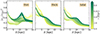 |
Fig. E.1. Radial profiles of vertical-to-radial velocity dispersion (σzz/σRR) for thin disc (left panels), thick disc stars (middle panels), and total (thin+thick) disc stars (right panels) as a function of time (shown in colour bar) for model rthickE0.5. |
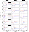 |
Fig. E.2. Temporal evolution of vertical-to-radial velocity dispersion (σzz/σRR) calculated within Rb/p, (σzz/σRR)2(t; R ≤ Rb/p) for thin (in blue), thick (in red), and total (thin+thick) disc (in black) particles, for all thin+thick-disc models. Left panels show the evolution for the rthickS models, whereas middle panels and right panels show the evolution for the rthickE and rthickG models, respectively. The thick-disc fraction (fthick) varies from 0.1 to 1 (top to bottom), as indicated in the left-most panel of each row. The vertical maroon dotted line denotes the onset of bar formation (τbar), while the vertical magenta dotted line denotes the onset of buckling instability (τbuck; for details, see text). |
All Tables
All Figures
|
Fig. 1. Edge-on density distribution of all disc particles (thin+thick) at the end of the simulation run (t = 9 Gyr) for all thin+thick disc models with varying fthick values. Black dotted lines denote the contours of constant density. Left panels show the density distribution for the rthickS models, whereas middle panels and right panels show the density distribution for the rthickE and rthickG models, respectively. The thick disc fraction (fthick) varies from 0.1 to 1 (top to bottom), as indicated in the left-most panel of each row. The bar is placed along the x-axis (side-on configuration) for each model. The vertical black dashed lines denote the extent of the b/p structure in each case (for details, see the text in Sect. 3.1.2). |
| In the text | |
|
Fig. 2. Radial profiles of median of absolute value of distribution of particles in vertical (z) direction, |
| In the text | |
|
Fig. 3. Temporal evolution of b/p strength, Sb/p, calculated using Eq. (1), for thin-disc (upper panels), thick-disc (middle panels), and total (thin+thick) disc stars (lower panels) for all thin+thick disc models with varying fthick values (see the colour bar). Left panels show the b/p strength evolution for the rthickS models, whereas middle panels and right panels show the b/p strength evolution for the rthickE and rthickG models, respectively. The thick disc fraction (fthick) varies from 0.1 to 0.9 (with a step-size of 0.2), as indicated in the colour bar. The blue solid lines in the middle and the bottom rows denote the three thick-disc-only models (fthick = 1), whereas the red solid line in the top middle panel denotes the thin-disc-only model (fthick = 0; for details, see text). |
| In the text | |
|
Fig. 4. Growth rate of b/p, dSb/p/dt, as a function of time for three thin+thick models with fthick = 0.5. All the stellar particles (thin+thick) are considered here in each model. The growth rate is steeper in rthickS0.5 model when compared with that for other two configurations with same fthick value. |
| In the text | |
|
Fig. 5. Strength of b/p, Sb/p (top panel), and extent of b/p, Rb/p (bottom panel), calculated using thin+thick disc particles, at t = 9 Gyr shown as a function of thick-to-total mass fraction (fthick) and for different geometric configurations. With increasing fthick value, the b/ps progressively become weaker and larger in extent, and this trend remains true for all three geometric configurations considered here. The errors are calculated by constructing a total of 5000 realisations by resampling the entire population via a bootstrapping technique (for details, see text). |
| In the text | |
|
Fig. 6. Temporal variation of b/p extent, Rb/p, calculated using thin-, thick-disc, and thin+thick disc particles for model rthickE0.5. The b/p extent increases by a factor of ∼2 over the total simulation runtime. At t = 9 Gyr, the thick-disc b/p remains a bit larger than the thin disc b/p. The errors on Rb/p are estimated by constructing a total of 5000 realisations by resampling the entire population via a bootstrapping technique (for details, see text). |
| In the text | |
|
Fig. 7. Quantifying the vertical asymmetry in thin+thick models. Left panel: temporal evolution of A1, z (Eq. (2)) denoting vertical asymmetry in bar region, calculated using thin-disc (blue lines), thick-disc (red lines), and thin+thick disc (black lines) for the model rthickE0.5. Right panel: temporal evolution of buckling amplitude, Abuck (Eq. (3)), calculated using thin-disc (blue lines), thick-disc (red lines), and thin+thick disc (black lines) for the model rthickE0.5. The vertical magenta dotted line denotes the onset of buckling instability (τbuck), calculated from the peak of Abuck profile (for details, see text). Furthermore, for reference, we indicate the onset of bar formation (τbar, vertical maroon dotted line), calculated from the amplitude of the m = 2 Fourier moment. |
| In the text | |
|
Fig. 8. Distribution of mid-plane asymmetry, AΣ(x, z), in the edge-on projection (x − z-plane), computed separately for the thin (left columns) and thick (middle columns) discs, as well as thin+thick (right columns) disc particles using Eq. (4) at six different times (before and after the buckling event) for the model rthickE0.5. The bar is placed along the x-axis (side-on configuration) for each time-step. Black lines denote contours of constant density. A mid-plane asymmetry persists, even long after the model has gone through the buckling phase. |
| In the text | |
|
Fig. 9. Bar-b/p strength correlation: distribution of all thin+thick models in maximum bar strength – maximum b/p strength plane. The maximum bar strengths are taken from Ghosh et al. (2023), whereas the maximum b/p strengths are determined from Eq. (1). The colour bar denotes the thick-disc mass fraction (fthick). Different symbols represent models with different geometric configurations (see the legend). The maximum strength of the bar correlates overall with the maximum b/p strength, and this remains true for all three geometric configurations. |
| In the text | |
|
Fig. 10. Variation of b/p extent with varying thick-disc mass fraction. Top panel: temporal evolution of ratio of b/p length (Rb/p) and bar length (Rbar) for model rthickE0.5. Bottom panel: variation of ratio of b/p and bar length, calculated at the end of the simulation run (t = 9 Gyr), with thick-disc mass fraction (fthick). |
| In the text | |
|
Fig. 11. Variation of time delay between the formation and onset of buckling instability, τbuck − τbar, with thick-disc mass fraction (fthick), for all thin+thick models considered here. For a fixed geometric configuration, τbuck − τbar becomes progressively shorter with increasing fthick values (for details, see text). |
| In the text | |
|
Fig. 12. Quantifying the kinematic signature of teh vertical buckling instability and the subsequent b/p formation. Left panel: temporal evolution of vertical-to-radial velocity dispersion (σzz/σRR), calculated within the b/p extent (Rb/p), (σzz/σRR)2(t; R ≤ Rb/p), for thin (in blue), thick (in red), and total (thin+thick) disc (in black) particles, for model rthickE0.5. Right panel: temporal evolution of meridional tilt angle (Θtilt), calculated within Rb/p using Eq. (7), for thin (in blue), thick (in red), and total (thin+thick) disc (in black) particles, for model rthickE0.5. The vertical maroon dotted line denotes the onset of bar formation (τbar), while the vertical magenta dotted line denotes the onset of buckling instability (τbuck; for details, see text). |
| In the text | |
|
Fig. 13. Variation of the b/p morphology with varying thick-disc mass faction (fthick). Top left panels: density contours of edge-on stellar (thin+thick) distribution (with bar placed along the x-axis) in central region at t = 9 Gyr for models rthickE0.1 and rthickE0.9. For the rthickE0.1 model, the contours display more prominent X-shaped feature, whereas for the rthickE0.9 model, the contours display more prominent box-shaped feature. Bottom left panels: density profiles (normalised by the peak density value, and in log-scale) along bar major axis, calculated at different heights (from |z| = 0 to 6 kpc, with a step-size of 1 kpc) from mid-plane, for models rthickE0.1 and rthickE0.9. The density profiles have been artificially shifted along the y-axis to show the trends as height changes, and they do not overlap. Right panel: vertical stellar density distribution (normalised by the peak density value, and in log-scale), at a radial location around peak of the b/p structure (marked by blue vertical lines in top left panels) for rthickE0.1 and rthickE0.9 models. |
| In the text | |
|
Fig. 14. Fraction of thin-disc stars, fthin(=1 − fthick), in the edge-on projection (with the bar placed along the x-axis) compared to the total (thin+thick) disc, at the end of the simulation run (t = 9 Gyr) for all thin+thick disc models with varying fthick values. Left panels show the distribution for the rthickS models, whereas middle panels and right panels show the distribution for the rthickE and rthickG models, respectively. The values of (fthick) vary from 0.1 to 0.9 (top to bottom), as indicated in the left-most panel of each row. For each model, the fraction of thin-disc stars decreases with height from the mid-plane (z = 0). In addition, the appearance of the b/p structure changes from more X-shaped to more boxy-shaped as the thick-disc mass fraction steadily increases. |
| In the text | |
|
Fig. A.1. Temporal evolution of C2, z, b/p strength computed from the Fourier decomposition using Eq. A.1, plotted against the b/p strength calculated using Eq. 1 for the model rthickE0.5. All the stellar particles (thin+thick) within the b/p extent (Rb/p) are used in both cases. The colour bar denotes the time of the simulation. Both the measures of b/p strength correlate fairly well. |
| In the text | |
|
Fig. B.1. Comparison of different methods for measuring the b/p extent. Top panel: Profiles of function Dg(x, z) (see Eq. (B.1)), calculated at three different times for model rthickE0.5. The horizontal dotted line denotes the zeros of the function Dg(x, z) (for details, see text). Bottom panel: Correlations between size of the b/p, Lb/p and the b/p length Rb/p for the model rthickE0.5. A straight line of the form Y = AX + B is fitted (black dashed line), and the corresponding best-fit parameters are quoted. The Pearson correlation coefficients are quoted (see top right). Here, Rd, thin = 4.7 kpc. |
| In the text | |
|
Fig. C.1. B/p extent, at the end of the simulation run (t = 9 Gyr), computed for the thin and thick discs, as well as for the thin+thick case, for all the thin+thick models considered here. Left panels show the distribution for the rthickS models, whereas middle panels and right panels show the distribution for the rthickE and rthickG models, respectively. Thin disc b/ps always remain shorter than the thick disc b/ps. The errors on Rb/p are estimated by constructing a total of 5,000 realisations by resampling the entire population via a bootstrapping technique (for details, see Sect. 3.1.2). |
| In the text | |
|
Fig. D.1. Variation of bar formation epoch, τbar, as a function of thick-disc mass fraction (fthick), for all thin+thick models considered here. For a given geometric configuration, the bar formation epoch increases with increasing fthick values, and this holds true for all three geometric configurations considered here. |
| In the text | |
|
Fig. E.1. Radial profiles of vertical-to-radial velocity dispersion (σzz/σRR) for thin disc (left panels), thick disc stars (middle panels), and total (thin+thick) disc stars (right panels) as a function of time (shown in colour bar) for model rthickE0.5. |
| In the text | |
|
Fig. E.2. Temporal evolution of vertical-to-radial velocity dispersion (σzz/σRR) calculated within Rb/p, (σzz/σRR)2(t; R ≤ Rb/p) for thin (in blue), thick (in red), and total (thin+thick) disc (in black) particles, for all thin+thick-disc models. Left panels show the evolution for the rthickS models, whereas middle panels and right panels show the evolution for the rthickE and rthickG models, respectively. The thick-disc fraction (fthick) varies from 0.1 to 1 (top to bottom), as indicated in the left-most panel of each row. The vertical maroon dotted line denotes the onset of bar formation (τbar), while the vertical magenta dotted line denotes the onset of buckling instability (τbuck; for details, see text). |
| In the text | |
Current usage metrics show cumulative count of Article Views (full-text article views including HTML views, PDF and ePub downloads, according to the available data) and Abstracts Views on Vision4Press platform.
Data correspond to usage on the plateform after 2015. The current usage metrics is available 48-96 hours after online publication and is updated daily on week days.
Initial download of the metrics may take a while.