| Issue |
A&A
Volume 674, June 2023
|
|
|---|---|---|
| Article Number | A128 | |
| Number of page(s) | 20 | |
| Section | Extragalactic astronomy | |
| DOI | https://doi.org/10.1051/0004-6361/202245275 | |
| Published online | 13 June 2023 | |
Bars and boxy/peanut bulges in thin and thick discs
II. Can bars form in hot thick discs?
1
Max-Planck-Institut für Astronomie, Königstuhl 17, 69117 Heidelberg, Germany
e-mail: This email address is being protected from spambots. You need JavaScript enabled to view it.
2
Institute for Computational Cosmology, Department of Physics, Durham University, South Road, Durham DH1 3LE, UK
3
GEPI, Observatoire de Paris, PSL Research University, CNRS, Sorbonne Paris-Cité, 5 place Jules Janssen, 92190 Meudon, France
4
Inter-University Centre for Astronomy and Astrophysics, Post Bag 4, Ganeshkhind, Pune, Maharashtra 411007, India
Received:
24
October
2022
Accepted:
17
April
2023
Abstract
The Milky Way and a majority of external galaxies possess a thick disc. However, the dynamical role of the (geometrically) thick disc in the bar formation and evolution is not fully understood. Here, we investigate the effect of thick discs in the formation and evolution of bars by means of a suite of N-body models of (kinematically cold) thin and (kinematically hot) thick discs. We systematically varied the mass fraction of the thick disc, the thin-to-thick disc scale length ratio, and the thick disc scale height to examine the bar formation under diverse dynamical scenarios. Bars form almost always in our models, even in the presence of a massive thick disc. The part of the bar that consists of the thick disc closely follows the overall growth and temporal evolution of the part of the bar that consists of the thin disc, but the part of the bar in the thick disc is weaker than the part of the bar in the thin disc. The formation of stronger bars is associated with a simultaneous greater loss of angular momentum and a more intense radial heating. In addition, we demonstrate a preferential loss of angular momentum and a preferential radial heating of disc stars in the azimuthal direction within the extent of the bar in both thin and thick disc stars. For purely thick-disc models (without any thin disc), the bar formation critically depends on the disc scale length and scale height. A larger scale length and/or a larger vertical scale height delays the bar formation time and/or suppresses the bar formation almost completely in thick-disc-only models. We find that the Ostriker-Peeble criterion predicts the bar instability scenarios in our models better than the Efstathiou-Lake-Negroponte criterion.
Key words: galaxies: kinematics and dynamics / galaxies: structure / galaxies: spiral / methods: numerical / galaxies: evolution
© The Authors 2023
 Open Access article, published by EDP Sciences, under the terms of the Creative Commons Attribution License (https://creativecommons.org/licenses/by/4.0), which permits unrestricted use, distribution, and reproduction in any medium, provided the original work is properly cited.
This article is published in open access under the Subscribe to Open model.
Open access funding provided by Max Planck Society.
1. Introduction
Stellar bars are one of the most abundant non-axisymmetric structures in disc galaxies. About two-thirds of the disc galaxies in the local Universe harbour stellar bars, as revealed by various optical and near-infrared surveys of galaxy morphology (e.g., see Eskridge et al. 2000; Whyte et al. 2002; Aguerri et al. 2009; Nair & Abraham 2010; Masters et al. 2011; Kim et al. 2015; Kruk et al. 2017), and about one-third of them host strong bars. The bar fraction varies strongly with the stellar mass (e.g., Nair & Abraham 2010) or Hubble type (e.g., Aguerri et al. 2009; Buta et al. 2010; Nair & Abraham 2010; Barway et al. 2011) of the host galaxies. The question remains whether the remaining one-third of the disc galaxies in the local Universe are hostile to bar formation and their subsequent growth, or if bars are destroyed during their evolutionary pathway.
Much of our current understanding of the bar formation and its growth in disc galaxies was gleaned from numerical simulations. Several studies using N-body simulations have shown that an axisymmetric disc galaxy forms a bar spontaneously when the disc becomes unstable to the formation of a bar. When a bar forms, orbits that are close to circular become more elongated, with the bar being comprised of elongated orbits (which are called the x1 family of orbits; e.g., see Contopoulos & Grosbol 1989; Martinez-Valpuesta et al. 2006). Previous theoretical studies have shown that a massive central mass concentration and/or inflow of the interstellar gas in the central region can weaken/destroy stellar bars (e.g., see Pfenniger & Norman 1990; Shen & Sellwood 2004; Athanassoula et al. 2005, 2013; Bournaud et al. 2005; Hozumi & Hernquist 2005). While in principle, these mechanisms can lead to the (complete) destruction of bars, they might still require a very high central mass concentration or prodigious amount of gas inflow (Athanassoula et al. 2005). Furthermore, recent work by Ghosh et al. (2021) demonstrated that a minor merger can also lead to a substantial weakening of stellar bars, and in some cases, cause even a complete destruction of stellar bars in the host galaxies.
On the other hand, a disc galaxy might be dynamically hot enough, or equivalently, have a higher value of the Toomre Q parameter to prevent the bar instability, which in turn causes a disc galaxy to remain unbarred throughout its lifetime (e.g., see Toomre 1964; Binney & Tremaine 2008). Moreover, a (rigid) compact and dense dark matter halo was thought to suppress the bar instability in a disc galaxy (e.g., Mihos et al. 1997). Later N-body studies in which the dark matter halo was treated as live, revealed the opposite trend, that is, disc galaxies with a higher halo concentration develop a much stronger, larger, and thinner bar; however, the bar formation is still delayed (e.g., see Debattista & Sellwood 1998, 2000; Athanassoula & Misiriotis 2002; Athanassoula 2003).
Several theoretical efforts have been made towards determining the dynamical condition for a disc to become bar-unstable. Earlier works of Ostriker & Peebles (1973) showed that a stellar disc would enter into the bar instability phase if the ratio of the rotational kinetic energy to the potential energy, W, exceeds a critical limit of 0.14 ± 0.003. This criterion has been tested further in recent N-body simulation (e.g., see Saha & Elmegreen 2018). On the other hand, Efstathiou et al. (1982), using 2D N-body simulations (with a rigid dark matter halo), proposed an analytic criterion for the global stability of cold exponential stellar discs. To illustrate this, a disc becomes bar-stable if the dimensionless quantity  becomes greater than 1.1, where Vmax is the maximum rotational velocity, Mdisc is the total disc mass, and
  is the inverse of the disc scale length (Efstathiou et al. 1982). Later, this criterion has been tested in context of galaxies from the cosmological zoom-in simulations as well as for the observed galaxies (e.g., see the recent works of Izquierdo-Villalba et al. 2022; Romeo et al. 2023).
Bars are present in the high-redshift galaxies as well. However, some studies claimed a decreasing bar fraction with increasing redshift (e.g., see Sheth et al. 2008; Melvin et al. 2014; Simmons et al. 2014), while some other studies showed a constant bar fraction up to redshift z ∼ 1 (e.g., Elmegreen et al. 2004; Jogee et al. 2004). Hence, the fraction of galaxies in the high-redshift hosting bar still remains debated. In addition, cosmological simulations find that bars already start to form at z ∼ 1 (e.g., see Kraljic et al. 2012; Fragkoudi et al. 2020, 2021; Rosas-Guevara et al. 2022). Furthermore, the recent photometric study by Guo et al. (2023) using the rest-frame near-infrared images from the James Webb Space Telescope (JWST), unveiled the presence of stellar bars in disc galaxies at high redshifts (z > 1). At high redshift, discs are known to be thick, kinematically hot (and turbulent), and more gas rich. The question therefore remains whether bars can form in these thick discs.
The existence of a thick-disc component is now observationally well established in the Milky Way and in external galaxies (e.g., see Tsikoudi 1979; Burstein 1979; Gilmore & Reid 1983; Yoachim & Dalcanton 2006; Comerón et al. 2011a,b, 2018). For external galaxies, thick discs are found along the whole Hubble sequence, from early-type S0 galaxies (Pohlen et al. 2004; Kasparova et al. 2016; Comerón et al. 2016; Pinna et al. 2019b,a) to late-type galaxies (Yoachim & Dalcanton 2006; Comerón et al. 2019; Martig et al. 2021; Scott et al. 2021). The thick-disc component is in general vertically more extended and kinematically hotter than the thin-disc component (e.g., see Jurić et al. 2008; Bovy et al. 2012, 2016; Vieira et al. 2022). Recent studies of the chemical evolution of α-enhanced stars in the Milky Way indicated that the mass of the chemically thick disc can be of the same order as that of the thin disc (e.g., Haywood et al. 2013; Snaith et al. 2015). Furthermore, Comerón et al. (2011a) argued that (geometrically) thick discs can constitute a significant fraction of the baryonic content of galaxies.
While significant efforts have been devoted towards understanding the bar instability scenario in disc galaxies, a majority of the N-body simulations considered a one-component stellar disc. A few studies in the past have investigated how the disc stars would become trapped in the bar instability as a function of how dynamical hot or cold the underlying population is (e.g., see Hohl 1971; Athanassoula & Sellwood 1986; Athanassoula 2003; Debattista et al. 2017). Aumer & Binney (2017) showed that the presence of a thick disc delays the bar formation. In addition, the study by Klypin et al. (2009) showed that N-body models with thick discs (scale height-to-length ratio = 0.2) produce very long and slowly rotating bars. Furthermore, Fragkoudi et al. (2017) studied the effect of this thick disc component on the bar and the boxy/peanut formation using a fiducial two-component thin+thick model where the thick disc constitutes 30% of the total stellar mass. However, a systematic study of the bar formation in disc galaxies with different hot and cold discs, as well as composite thin and thick discs, is still lacking. We aim to address this here.
In this work, we systematically investigate the dynamical role of the thick-disc component in the bar formation and growth by making use of a suite of N-body models with (kinematically cold) thin and (kinematically hot) thick discs. Within the suite of N-body models, we vary the thick-disc mass fraction and consider different geometric configurations (a varying ratio of the thin- and thick-disc scale lengths). Furthermore, for some models, we vary the disc scale height as well (while keeping the scale length fixed) to examine the bar formation scenario in these cases. We quantify the strength and growth of the bars in thin- and thick-disc stars, and we also study the underlying dynamical mechanisms, such as angular momentum transport and radial heating within the bar region. In addition, we test some of the most commonly used bar instability criteria, as mentioned before, in the suite of N-body models considered here.
The rest of the paper is organised as follows. Section 2 provides the details of the simulation set-up and the initial equilibrium models. Section 3 quantifies the properties of the bars in different models and the associated temporal evolution, while Sect. 4 discusses the effect of the disc scale height on the bar formation. Section 5 provides the details of the angular momentum transport and the radial heating within the bar region. Section 6 contains the results related to applying a few instability criteria on the thin+thick disc models considered here. Section 7 contains the discussion, and Sect. 8 summarizes the main findings of this work.
2. Simulation set-up and N-body models
To motivate our study, we developed a suite of N-body models, consisting of a thin and a thick stellar disc. The whole system was embedded in a live dark matter halo. One such model has been presented in Fragkoudi et al. (2017). Here, we built a suite of numerical models of thin+thick discs while systematically varying the thick-disc mass fraction as well as the ratio of the thick-to-thin disc scale lengths.
Each of the thin and thick discs is modelled with a Miyamoto–Nagai profile whose potential has the form (Miyamoto & Nagai 1975)
 (1)
(1)
where Rd and zd are the characteristic disc scale length and scale height, respectively, and Md is the total mass of the disc. The dark matter halo is modelled with a Plummer sphere whose potential has the form (Plummer 1911)
 (2)
(2)
where RH is the characteristic scale length, and Mdm is the total halo mass. Here, r and R are the radius in the spherical and the cylindrical coordinates, respectively. The values of the key structural parameters for the thin and thick discs as well as the dark matter halo are listed in Table 1. The total number of particles used to model each of these structural components is also listed in Table 1.
Key structural parameters for the equilibrium models.
The initial conditions of the discs were obtained using the iterative method algorithm (see Rodionov et al. 2009). This algorithm constructs equilibrium-phase models for stellar systems by making use of a constrained evolution in such a way that the equilibrium solution has the number of desired parameters. For this work, we only constrained the density profile of the stellar discs (following Eq. (1)) while allowing the velocity dispersions (of the radial and vertical components) to vary in such a way that the system converged to an equilibrium solution (for details, see Fragkoudi et al. 2017).
In the initial equilibrium set-up for the thin+thick disc models, we considered three different scenarios for the scale lengths of the two disc (thin and thick) components. In rthickE models, the scale lengths of the thin and thick discs are kept same (Rd, thick = Rd, thin), whereas in rthickG models, the scale length of the thick disc component is larger than that for the thin disc (Rd, thick > Rd, thin). In rthickS models, the scale length of the thick-disc component is shorter than that for the thin disc (Rd, thick < Rd, thin). For each of these three configurations, the fraction of total stellar particles that are in the thick disc component (fthick)1 was systematically varied from 0.1 to 0.9 (with a step size of 0.2). Thus, we had a total of 15 such thin+thick models. We analyse them later in this work. In addition, we considered one purely thin-disc model (fthick = 0) and three purely thick-disc models (fthick = 1) to augment this study. Furthermore, to study the effect of the disc scale height on the bar formation (see Sect. 4), we constructed another six thick-disc-only models while varying the vertical scale height of the thick disc. The values of the key structural parameters for these six models are also listed in Table 1. Thus, we analysed a total of 25 N-body models for this work.
The simulations were run using the TreeSPH code by Semelin & Combes (2002). This code has been extensively used to simulate interacting and merging galaxies as well as isolated galaxies (e.g., Fragkoudi et al. 2017; Jean-Baptiste et al. 2017). The hierarchical tree method (Barnes & Hut 1986) with a tolerance parameter2θ = 0.7 was employed to calculate the gravitational force, which includes terms up to the quadrupole order in the multipole expansion. A Plummer potential was used to soften the gravitational forces with a softening length ϵ = 150 pc. The equations of motion were integrated using the leapfrog algorithm (Press et al. 1986) with a fixed time step of Δt = 0.25 Myr. All the models considered here were evolved for a total time of 9 Gyr.
For consistency, any thin+thick model is referred to as a unique string ‘[MODEL CONFIGURATION][THICK DISC FRACTION]’. [MODEL CONFIGURATION] denotes the corresponding thin-to-thick disc scale length configuration, that is, rthickG, rthickE, or rthickS, whereas [THICK DISC FRACTION] denotes the fraction of the total disc mass that is in the thick-disc population. To illustrate this, rthickG0.3 denotes the model in which the scale length of the thick-disc component is larger than that for the thin disc, and 30% of the total disc mass is in the thick-disc component. The purely thin-disc-only model is referred to as rthick0.0, and the purely thick-disc-only models are referred to as rthickS1.0, rthickE1.0, and rthickG1.0. Similarly, the six thick-disc-only models (in which we varied the scale height) are referred to as rthickE1.0zd2.3, rthickG1.0zd2.3, rthickE1.0zd4.7, rthickE1.0zd4.7, and rthickG1.0zd5.6. To illustrate this, rthickS1.0zd2.3 denotes a thick-disc-only model with the thick disc scale height set to 2.3 kpc (while keeping the other parameters unchanged), and so on.
3. Formation and evolution of the bar for different thick-disc mass fractions
Before we present the results, we mention that we can identify and separate by construction in our thin+thick disc models the stars that are are members of the thin-disc and the thick-disc component, and we can track them as the system evolves self-consistently. Throughout this paper, we therefore refer to the bar as seen exclusively in the thin-disc population as the thin-disc bar, or equivalently, the bar in the thin disc, and the bar seen exclusively in the thick-disc population as the thick-disc bar, or equivalently, the bar in the thick disc.
Figure 1 shows the density distribution of all stars (thin+thick) in the face-on projection (x − y-plane) for all thin+thick disc models (with fthick varying from 0.1 to 1) considered here, at the end of the simulation run (t = 9 Gyr). Even a mere visual inspection reveals that almost all the models develop a strong bar by 9 Gyr. We further checked the same face-on density distribution, computed separately for thin and thick disc stars. Both of them show a prominent bar. For the sake of brevity, we do not show it here (however, see Fig. 2 in Fragkoudi et al. 2017).
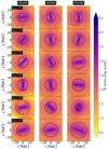 |
Fig. 1. Face-on density distribution of all disc particles (thin+thick) at the end of the simulation run (t = 9 Gyr) for all thin+thick disc models with varying fthick values. The white solid lines denote the constant density contours. The solid black circle in each sub-panel denotes the corresponding extent of the bar (Rbar). Left panels: density distribution for the rthickS models, and the middle and right panels: density distribution for the rthickE and rthickG models, respectively. The thick disc fraction (fthick) varies from 0.1 to 1 (top to bottom), as indicated in the left-most panel of each row. A prominent bar forms in almost all models considered here. |
To quantify the strength of the bars in the thin- and thick-disc components of our models, we first computed the radial profiles of the m = 2, 4, 6 Fourier coefficients using (e.g., see Saha & Elmegreen 2018; Ghosh et al. 2021)
 (3)
(3)
where Am is the coefficient of the mth Fourier moment of the density distribution, mi is the mass of the ith particle, and ϕi is its cylindrical angle. The summation runs over all the particles within the radial annulus [R, R + ΔR], with ΔR = 0.5 kpc. In Fig. 2 we show the corresponding radial profiles of m = 2, 4, 6 Fourier coefficients for the thin, thick, and thin+thick discs as a function of time for the model rthickE0.5. The prominent peak in the A2/A0 radial profiles, accompanied by a similar peak (but with a lower peak value) in the A4/A0 radial profiles clearly confirms the presence of a strong, central stellar bar in the thin- and thick-disc components. Moreover, the peaks in the radial profiles of the m = 2, 4, 6 Fourier coefficients shift towards the outer regions at later times, indicating that the peak of the non-axisymmetry moves towards larger radii as time progresses. This trend is present in the thin- and the thick-disc component. Furthermore, at later times, the radial profiles of the m = 2 Fourier coefficient show multiple peaks that are spatially well separated. We verified that the outward shift of the peaks in the radial profiles of the Fourier coefficients as well as the presence of multiple peaks in the m = 2 profiles are seen in other thin+thick disc models as well. These models develop a prominent boxy/peanut structure at later times (for details, see Fragkoudi et al. 2017). The formation of multiple peaks might be linked to the formation of a 3D boxy/peanut structure, as demonstrated in Saha et al. (2018) and Vynatheya et al. (2021). The details of the boxy/peanut formation and their properties are beyond the scope of this paper and will be taken up in a future work.
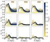 |
Fig. 2. Radial profiles of the m = 2, 4, 6 Fourier coefficients (normalised by the m = 0 component), for the thin disc (left panels), thick-disc stars (middle panels), and total (thin+thick) disc stars (right panels) as a function of time (shown in the colour bar) for the model rthickE0.5. At later times, the peaks of the radial profiles of the m = 2, 4, 6 Fourier coefficients shift towards the outer regions. |
Next, we studied the temporal evolution of the strength of the bars in thin and thick disc separately, and also for the thin and thick disc combined. At any time t, we defined the strength of the bar, Sbar, as the peak value of the m = 2 Fourier coefficient (A2/A0). The resulting temporal variation in the bar strength of the thin and thick discs and of the thin+thick disc are shown in Fig. 3 for all models considered here. Figure 3 clearly shows that regardless of the geometric configuration, that is, the scale length of the thick disc with respect to the scale length of the thin disc, the temporal evolution of the bar strength in the thick-disc component closely follows that for the bar in the thin-disc component. However, the bar in the thick-disc component remains weaker than the bar in the thin-disc component; this remains true for all times and for all the thin+thick models considered here. This agrees with the earlier findings of Fragkoudi et al. (2017). The temporal evolution of Sbar for the model rthickG0.9 merits some discussion. The bar strength for model rthickG0.9 is weaker than for the other rthickG models, as revealed by the values of Sbar.
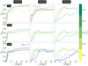 |
Fig. 3. Temporal evolution of the bar strength, Sbar, for the thin-disc (upper panels), thick-disc (middle panels), and total (thin+thick) disc stars (lower panels) for all thin+thick disc models with varying fthick values (see the colour bar). Left panels: bar strength evolution for the rthickS models, and the middle and right panels: evolution of the bar strength for the rthickE and rthickG models, respectively. The thick-disc fraction (fthick) varies from 0.1 to 0.9 (with a step size of 0.2), as indicated in the colour bar. The solid blue lines in the bottom row denote the three thick-disc-only models (fthick = 1), and the solid red line in the top middle panel denotes the thin-disc-only model (fthick = 0). For details see text. |
The thin-disc-only (rthick0.0) model also develops a prominent bar during the evolution, similar to other thin+thick models. The bar forms quite early on (within ∼2 Gyr), grows for a certain time, and then saturates (see Fig. 3). For the thick-disc-only models, all three models, namely, rthickS1.0, rthickE1.0, and rthickG1.0, form a prominent bar by the end of the simulation run. However, the bar in the rthickG1.0 remains weaker than that in the other two thick-disc-only models (see Fig. 3).
To further quantify the epoch of bar formation and how fast the bar grows in an individual model, we defined the growth rate, dSbar/dt, as the time derivative of the strength of bar. The resulting variation in the growth rate as a function of time is shown in Fig. 4 for thin-, thick-, and thin+thick disc particles for all models. In the thin and thick discs, the bar displays a fast growth phase at initial times, followed by one/multiple buckling phases (for details of the buckling instability, see, e.g., Combes et al. 1990; Martinez-Valpuesta et al. 2006), as indicated by the prominent dip (negative values) in the temporal evolution of dSbar/dt. However, at later times (t > 6 Gyr), the bars no longer grow, as indicated by dSbar/dt ∼ 0, and remain as a steady non-axisymmetric feature. We found no time lag between the epochs of bar formation (or bar growth) in the thin and thick discs. Furthermore, a careful inspection of Figs. 3 and 4 reveals that the bars in most of the rthickS configuration form at an earlier epoch than in the other two configurations considered here. Moreover, during the initial rapid bar formation phase, the bars in the rthickS configuration grow at a much faster rate than the bars in other two configurations, and this trend holds for almost all fthick values considered here.
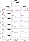 |
Fig. 4. Temporal evolution of the growth/decay rate of the bar strength (dSbar/dt), for the thin-, thick-, and total (thin+thick) disc components for all models with varying fthick values. Left panels: evolution for the rthickS models, and the middle and right panels: evolution for the rthickE and rthickG models, respectively. The fthick values are indicated in the left-most panel of each row. Top middle row: growth/decay rate of the bar strength for the thin-disc-only model (fthick = 0). |
In addition, the temporal evolution of dSbar/dt for the three thick-disc-only models (see the bottom panels of Fig. 4) reveals that the bar in the rthickG1.0 model forms at a much later time (∼6.1 Gyr), while the bar in the rthickS1.0 model forms at a much earlier time (within ∼1 Gyr). Thus, for the rthickS models, the bar seems to grow fast and become quite strong regardless of the mass of the thick disc. The rthickS model with 90% of the mass in the thick disc still forms a bar. This is also true for the case in which 100% of the mass is in the thick disc. This demonstrates that centrally concentrated discs are unstable to bar formation even when they are kinematically hot. As the disc scale length increases (in rthickE and rthickG models), the bar formation epoch is progressively delayed and also results in forming a progressively weaker bar.
4. Effect of the disc scale height on the formation of a bar
Here, we examine the effect of an increased disc scale height that therefore makes the disc kinematically hotter (in vz) on bar formation for the thick-disc-only models. To achieve this, we investigated the growth and evolution of the bar strength in the six thick-disc-only models by varying the disc scale height (for details, see Sect. 2).
We calculated the temporal evolution of the bar strength, Sbar for these six models. This is shown in Fig. 5. Now, we considered Sbar = 0.2 as the (operational) definition for denoting the onset of the bar, as has commonly been done in the literature (see e.g., Ghosh et al. 2021, and references therein). When we applied this criterion, we found that the model rthickS1.0zd2.3 developed a weak bar (with Sbar ∼ 0.2) at about 9 Gyr. For the other five models, the Sbar values lie below about 0.1, thereby confirming that these model do not form a central bar in 9 Gyr. However, for some these models, the temporal evolution of Sbar increased (with a much shallower slope dSbar/dt), thereby indicating that they might form a bar at later times (> 9 Gyr).
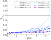 |
Fig. 5. Temporal evolution of the bar strength Sbar for the six thick-disc-only models with a varying vertical scale height. For details, see the text. The solid line denotes the rthickE models, the dashed line denotes the rthickG models, and the dotted line denotes the rthickS models. Different line colours denote models with different scale-height values. With increasing vertical scale height, the models progressively become bar stable. The horizontal line denotes Sbar = 0.2 and is used as a (operational) limit for the onset of bar formation. |
To conclude, the bar formation is delayed in presence of a much more vertically extended thick disc. This scenario is drastically different from the models rthickS1.0 and rthickG1.0, which form a prominent bar by the end of the simulation (compare Figs. 3 and 5) even though the entire stellar population is in the thick-disc component (i.e. fthick = 1). We calculated the radial profiles of the velocity dispersion in the radial as well as in the vertical directions for these six models. With increasing scale height of the disc, the corresponding vertical velocity dispersion also increased monotonically (see e.g., van der Kruit & Freeman 2011), while the radial velocity dispersion remained almost unchanged. For the sake of brevity, they are not shown here. This demonstrates the vital dynamical effect of the vertical scale height and hot vertical kinematics in the context of the bar formation scenario, in agreement with past findings (e.g., see Combes et al. 1990; Athanassoula 2003). A similar scenario of the suppression of the non-axisymmetric instability with increasing disc scale height is also seen for spiral arms (Ghosh & Jog 2018, 2022).
5. Angular momentum exchange and radial heating within the bar region
It is known that a stellar bar grows in a disc galaxy by transferring angular momentum from the disc to the dark matter halo. This transfer preferentially occurs at the resonance points of the bar (e.g., see Tremaine & Weinberg 1984; Hernquist & Weinberg 1992; Debattista & Sellwood 2000; Athanassoula & Misiriotis 2002; Sellwood & Debattista 2006; Dubinski et al. 2009; Saha & Naab 2013). Conversely, the weakening/destruction of a bar is associated with the gain in the angular momentum in the central region of disc galaxies (e.g., see Bournaud et al. 2005; Ghosh et al. 2021). At the same time, as a bar grows, it heats the disc through its action on the stars (e.g., see Saha et al. 2010; Saha 2014). Here, we quantify the change in the angular momentum content and the radial heating within the bar region as a function of time for all models (with varying fthick values) considered here.
Before we present the results related to the angular momentum transport and radial heating, we mention that for these analyses, we considered all stellar particles that currently lie within the extent of the bar (defined by Rbar) at a certain time t. In other words, we did not distinguish the stars that are a part of the bar and those that are only located within the bar region. The same scheme is applied throughout Sect. 5 and in the subsequent sections, unless defined otherwise.
5.1. Exchange of angular momentum
At time t, we calculated the z-component of the angular momentum (Lz) of the disc particles within the bar region using
![Mathematical equation: $$ \begin{aligned} L_z (t; R < R_{\rm bar}) = \sum _{i=1}^{N(t)} m_i \left[x_i(t) v_{{ y}_i}(t)- { y}_i(t) v_{x_i}(t)\right], \end{aligned} $$](/articles/aa/full_html/2023/06/aa45275-22/aa45275-22-eq6.gif) (4)
(4)
where N(t) is the total number of stellar particles contained within the bar region at time t, and x, y, vx, vy are the position and velocity of the particles. However, we point out that, in our thin+thick models, the fraction of particles assigned to the thin and thick disc changes in different models as the thick-disc fraction varies across models. Therefore, comparing Lz(t; R < Rbar) for various models (with different fthick values) will introduce certain biases as these quantities involved summation over all thin- and thick-disc particles within the bar region. For a uniform comparison among all the thin+thick models considered here, we therefore computed the specific angular momentum (lz) within the bar region using
![Mathematical equation: $$ \begin{aligned} l_z (t; R < R_{\rm bar}) = \frac{1}{N(t)}\sum _{i=1}^{N(t)} \left[x_i(t) v_{{ y}_i}(t)- { y}_i(t) v_{x_i}(t)\right]. \end{aligned} $$](/articles/aa/full_html/2023/06/aa45275-22/aa45275-22-eq7.gif) (5)
(5)
The resulting temporal evolution of lz within the bar region for the thin-, thick-, and total (thin+thick) disc particles is shown in Fig. 6 for all thin+thick disc models. During the total evolution time-span, the bar in the thin and thick disc grows substantially (by a factor of ∼2). Therefore, allowing Rbar to vary and then computing the specific angular momentum (lz) within the bar region (using Eq. (5)) essentially blurs the intrinsic changes in the specific angular momentum. However, in an individual model, after about 6 Gyr, the bar does not grow appreciably (see Fig. 3), and the values of Rbar also saturate, with occasional fluctuations. Therefore, we took this value as the representative value for Rbar for that particular model. One such Rbar determination for the model rthickE0.5 is further illustrated in Appendix A.
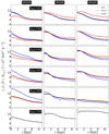 |
Fig. 6. Temporal evolution of the z-component of the specific angular momentum, calculated within the extent of the bar, lz(t; R < Rbar) (see Eq. (5)), for the thin- (in blue), thick- (in red), and total (thin+thick) disc (in black) particles for all thin+thick disc models. For each model, Rbar was first fixed to a saturation/representative value. For details, see Sect. 5.1. Left panels: evolution for the rthickS models, and the middle and right panels: evolution for the rthickE and rthickG models, respectively. The thick-disc fraction (fthick) varies from 0.1 to 1 (top to bottom), as indicated in the left-most panel of each row. The extents of bars in each sub-panel are as indicated in Fig. 1 (see the solid black circles there). |
Figure 6 clearly shows a substantial loss of specific angular momentum (within the central bar region, defined by the extent of Rbar) during the entire evolution of the bar. This trend remains true for the thin- and thick-disc components and for all the thin+thick models. The net loss in the specific angular momentum for the thin-disc component is always larger than that for the thick-disc component (as also discussed in Fragkoudi et al. 2017). In the initial rapid bar growth phase, the loss in the lz component is larger, but at later times (about t > 6 Gyr), when the bar remains steady, the loss in the lz component becomes negligible. This is true for the thin- and thick-disc particles and for all the thin+thick models considered here. For the thick-disc-only models, the loss of specific angular momentum (within the bar region) is progressively weaker from model rthickS1.0 to rthickE1.0 and to rthickG1.0 (see the bottom panels of Fig. 6). This matches the expectation because the formation of progressively weaker bars should be associated with progressively less angular momentum transfer from the central bar region.
While Fig. 6 clearly demonstrates that as the bar grows, there is an associated loss of the angular momentum in the central bar region (for thin and thick discs), it still remains unclear whether the loss in the lz component displays any characteristic azimuthal variation in the radial extent encompassing the bar. To investigate this, we computed the 2D distribution of the lz component in the face-on projection at five different times. Figure 7 shows one such distribution, computed using the thin-, thick-, and thin+thick disc particles for the model rthickE0.5. Figure 7 shows that along the bar, there is a prominent preferential deficiency of the specific angular momentum, and this holds true for the thin and thick disc. As the bar grows over time, this preferential deficiency in lz along the bar becomes more prominent (for the thin and thick disc). Moreover, the thin-disc component shows a larger deficiency of the specific angular momentum within the bar region than that for the thick-disc component (compare the left and middle panels of Fig. 7). This is expected because the bar in the thin-disc component is stronger than the bar in the thick-disc component, and a stronger bar is expected to transfer angular momentum more vigorously from the disc particles (as also discussed in Fragkoudi et al. 2017). We further computed the same 2D distribution of the lz component in the face-on projection at different times for all other thin+thick disc models considered here. We found that the trend of a preferential deficit of the specific angular momentum along the bar remains generic for all thin+thick models.
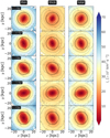 |
Fig. 7. Distribution of the z-component of the specific angular momentum in the face-on projection ((x, y)-plane) at different times for the thin- (left panels), thick- (middle panels), and thin+thick disc particles (right panels) for the model rthickE0.5. The dotted lines denote the contours of the total (thin+thick) surface density. The dashed black circle in each sub-panel denotes the extent of the bar. |
5.2. Radial heating of disc particles within the bar region
It is known from the literature that a bar heats the disc materials in the radial and vertical directions (e.g., see Grand et al. 2016; Pinna et al. 2018). However, here, we investigated how the disc particles in the inner part of the disc are heated as the bar grows over time. In the literature, the radial heating is quantified via radial random kinetic energy (ΠR), which is calculated (within the bar region) using
 (6)
(6)
where N(t) is the total number of stellar particles within the bar region at time t, and σR is the radial component of the velocity dispersion. However, this quantity is again a summation over thin- or thick-disc particles (whichever is applicable), and hence is prone to certain biases because the fthick values vary in our models (see the discussion in the last section). To circumvent this, we instead calculated the average radial random kinetic energy (⟨ΠR⟩) within the bar,
 (7)
(7)
The resulting temporal evolution of ⟨ΠR⟩3 within the bar region for the thin-, thick-, and total (thin+thick) disc particles is shown in Fig. 8 for all the thin+thick disc models and for the three thick-disc-only models. Figure 8 shows that initially, the thin disc remains kinematically colder than the thick disc. However, as the bar grows, the radial mean random kinetic energy for both the disc components (thin and thick) increases monotonically with time. At later times (t > 6 Gyr), when the bar no longer grows appreciably, the corresponding increment in the ⟨ΠR(t; R < Rbar)⟩ also becomes smaller. This holds true for both the thin and thick components. These overall trends in the temporal evolution of ⟨ΠR(t; R < Rbar)⟩ hold true for almost all the thin+thick models considered here. Interestingly, at the end of simulation (t = 9 Gyr), the average radial random kinetic energy for the thin and thick particles (within the bar region) becomes similar, although the thin disc was initially kinematically colder than the thick disc. A similar finding was also reported in Di Matteo et al. (2019). The only difference is that in their idealized model, the thin and thick disc initially share the same vertical velocity dispersion and differ in terms of the in-plane velocity dispersion. For the thick-disc-only models, the radial heating of stars within the bar region is progressively weaker from model rthickS1.0 to rthickE1.0 and to rthickG1.0 (see the bottom panels of Fig. 8). This is expected because the formation of progressively weaker bars is thought to be associated with progressively weaker radial disc heating in the central bar region.
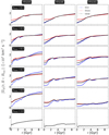 |
Fig. 8. Temporal evolution of the average radial random kinetic energy, calculated within the extent of the bar, ⟨ΠR(t; R < Rbar)⟩ (see Eq. (7)), for the thin- (in blue), thick- (in red), and total (thin+thick) disc (in black) particles for all thin+thick disc models. For each model, Rbar was first fixed to a saturation/representative value. For details, see Sect. 5.1. Left panels: evolution for the rthickS models, and the middle and right panels: evolution for models rthickE and rthickG, respectively. The value of fthick varies from 0.1 to 1 (top to bottom), as indicated in the left-most panel of each row. The extents of the bars in each sub-panel are indicated in Fig. 1 (see the solid black circles there). |
Next, we studied the 2D distribution of the change in the average random kinetic energy in the face-on projection. In particular, we searched for any characteristic variation in the average radial random kinetic energy along the bar. To quantify this, at any time t, we defined the change in the average radial random kinetic energy as
 (8)
(8)
In Fig. 9 we show the resulting variation in Δ⟨ΠR⟩(x, y, t) in the (x − y)-plane, calculated for the thin-, thick-, and thin+thick disc particles for model rthickE0.5. Figure 9 clearly shows a preferential excess of radial heating that traces the spatial 2D extent of the bar (in the face-on projection). This holds true for the thin- and the thick-disc components. When the bar is not very strong, the corresponding (preferential) increment of the average radial random kinetic energy is initially also small. Subsequently, as the bar grows with time, so does the radial random kinetic energy, and at the end of the simulation run (t = 9 Gyr), when the bar is fully grown, the corresponding radial random kinetic energy also reaches its maximum value. Within the bar region, the thin-disc particles are heated more strongly than the thick-disc particles. This confirms that the development of a stronger bar is associated with a higher degree of radial heating. We further confirmed this for the other thin+thick models as well. The preferential excess of radial heating along the bar (for the thin and thick components) remains a generic trend.
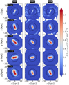 |
Fig. 9. Distribution of the change in the average radial random kinetic energy, Δ⟨ΠR⟩(x, y, t) (see Eq. (8)), calculated in the face-on projection ((x, y)-plane) at different times for the thin- (left panels), thick- (middle panels), and thin+thick disc particles (right panels) for model rthickE0.5. The dotted lines denote the contours of the total (thin+thick) surface density. The dashed black circle in each sub-panel denotes the extent of the bar. |
Lastly, we investigated the correlation (if any) between the changes in the specific angular momentum and the radial heating and the bar strength in the thin+thick models. To achieve this, we first computed the change in the specific angular momentum for the total (thin+thick) disc particles, within the bar region by using
 (9)
(9)
and then we also computed the change in the (average) radial heating within the bar region by using
 (10)
(10)
This is shown in Fig. 10. Figure 10 clearly shows that a stronger bar correlates with a higher angular momentum loss and a higher degree of radial heating for the stars. This trend holds for a wide variety of configurations (thin-to-thick disc scale-length ratio) and for different fthick values. This demonstrates that a stronger bar is associated with a larger amount of disc heating and a larger transfer of angular momentum from the disc particles, in agreement with previous findings (e.g., see Tremaine & Weinberg 1984; Debattista & Sellwood 2000; Saha et al. 2010; Grand et al. 2016).
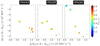 |
Fig. 10. Distribution of the change in average radial random kinetic energy and the specific angular momentum for the total (thin+thick) disc within the bar region (see Eqs. (9) and (10)) for all models considered here. Left panels: evolution for the rthickS models, and the middle and right panels: evolution for the rthickE and rthickG models, respectively. The points are colour-coded by the maximum value of the bar strength (Sbar, max). The increasing size of the points denotes a higher thick-disc fraction (fthick = 0.1 − 1). |
6. Testing the bar instability criteria
We tested two bar instability criteria that are widely used in the past literature on all the thin+thick models we considered to explore whether these criteria can indeed reveal when a bar will form. In Sect. 6.1 we investigated the Ostriker-Peebles (OP) criterion for the bar formation whereas in Sect. 6.2 we investigated the Efstathiou-Lake-Negroponte (ELN) criterion for the bar formation.
6.1. Ostriker-Peebles (OP) criterion
Using N-body simulations of disc galaxies, the seminal work by Ostriker & Peebles (1973) showed that a stellar disc would enter into the bar instability phase if the ratio of the total mean kinetic energy to the potential energy, W, exceeds a critical limit of 0.14 ± 0.003. Assuming that the virial theorem holds for our simulation snapshots, we can convert this criterion in terms of the rotational kinetic energy and the random kinetic energy. The random kinetic energy is calculated using
 (11)
(11)
where each component of the random kinetic energy is calculated as (Binney & Tremaine 2008)
 (12)
(12)
Here, j = R, ϕ, z; σj is the corresponding velocity dispersion, and m(i) is the mass of the ith disc particle. Similarly, the total mean kinetic energy is calculated as
 (13)
(13)
where each component of the mean kinetic energy is calculated as (Binney & Tremaine 2008)
 (14)
(14)
Here also, j = R, ϕ, z; ⟨vj⟩ is the corresponding mean velocity, and NR is the total number of particles in the radial extent [R, R + ΔR]. Now, following the tensor-virial theorem in a steady state, taking the trace of the kinetic and the potential tensors, we obtain (Binney & Tremaine 2008)
 (15)
(15)
Then, applying the OP criterion, we obtain (for details, see Saha & Elmegreen 2018)
 (16)
(16)
or equivalently,
 (17)
(17)
To explain this, if the ratio Π/Tmean is lower than 5.14, the stellar disc enters the bar instability phase, and if the ratio Π/Tmean is greater than 5.14, the corresponding stellar disc remains stable against the bar formation.
In Fig. 11 we show the ratio Π/Tmean, calculated at t = 0, within the extent of the bar, plotted against the maximum values of the bar strength for all 25 models we considered. The Π/Tmean(t = 0) values for the 15 thin+thick models that eventually develop a strong bar lie below 5.14, which means that the bar is unstable according to the OP criterion. The OP criterion also successfully predicts that the thick-disc-only models, namely rthickS1.0, rthickE1.0, and rthickG1.0, are bar unstable (with Π/Tmean(t = 0) < 5.14). However, the OP criterion fails to predict the bar stability scenario correctly for the thick-disc-only models, for which we increased the disc scale height. In other words, the Π/Tmean(t = 0) values for these models remain lower than 5.14, which means that the bar is unstable according to the OP criterion. However, most of these thick-disc-only models (with a larger scale height) do not form a prominent bar at all within the simulation run (9 Gyr). Nevertheless, we found an anti-correlation between the Π/Tmean(t = 0) values and the maximum bar strength (Sbar, max), which is expected in the sense that a system with lower Π/Tmean(t = 0) indeed develops a stronger bar in the disc (see Fig. 11). We further checked whether the temporal evolution of Π/Tmean(t) and the growth rate of the bar are correlated. This is shown in Fig. 12 for the models considered here. For most of the models, the growth rate of the bar clearly stabilises (i.e. dSbar/dt ∼ 0) after Π/Tmean(t) crosses the value 5.14. In other words, when the system eventually becomes bar stable according to the OP criterion, the bar does not grow drastically either (although it might enter the buckling phase). While this trend remains true for most of the models, Π/Tmean(t) remains low for the models that do not form a strong bar, for example, rthickG1.0 (bottom right panel in Fig. 12). One plausible explanation might be that because these models do not form a strong bar, the disc stars are not heated by the action of a (strong) bar. Hence, the total random kinetic energy remains low, which in turn keeps the ratio Π/Tmean lower than or closer to 5.14. In addition, for some models (see the bottom left panels of Fig. 12), the bar strength does not increase even though the values of Π/Tmean increase steadily.
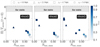 |
Fig. 11. Ostriker-Peeble (OP) criterion: ratio of the total mean kinetic energy to the total random kinetic energy, calculated within the extent of the bar, (Π/Tmean(t; R < Rbar)), at t = 0 for the total (thin+thick) disc as a function of the maximum bar strength (Sbar, max). Left panels: evolution for the rthickS models, and the middle and right panels: evolution for models rthickE and rthickG, respectively. The points are colour-coded by the corresponding thick-disc fraction, fthick (see the colour bar). Different symbols represent thin+thick models with different scale heights. For details, see the text. The shaded region denotes the bar-stable zone according to the OP criterion. |
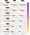 |
Fig. 12. Evolution of the ratio of the total mean kinetic energy to total random kinetic energy, calculated within the extent of the bar, (Π/Tmean(t; R < Rbar)), for the total (thin+thick) disc particles, plotted against the growth rate of the bar (dSbar/dt) for all thin+thick models with varying fthick values. Left panels: evolution for the rthickS models, and the middle and right panels: evolution for models rthickE and rthickG, respectively. The thick-disc fraction (fthick) varies from 0.1 to 1 (top to bottom), as indicated in the left-most panel of each row. The points are colour-coded by the simulation time (see the colour bar). The vertical black line denotes Π/Tmean = 5.14, which serves as a boundary for the bar instability phase, and the grey shaded region (in each sub-panel) denotes the bar-stable phase according to the OP criterion. For details, see the text. |
6.2. Efstathiou-Lake-Negroponte (ELN) criterion
Efstathiou et al. (1982) proposed an analytic criterion to determine the stability of a stellar disc against the bar formation:
 (18)
(18)
where vc, max is the maximum circular velocity, Mdisc is the total disc mass, and  , Rd is the scale length of the stellar disc. A stellar disc would become bar unstable for ε ≤ 1.1, and if ε > 1.1, the stellar disc would be stable against the bar formation (for details, see Efstathiou et al. 1982).
To compute ε at t = 0 for the total (thin+thick) disc, we first calculated the initial (t = 0) circular velocity profiles for the whole system and then determined the peak value of the circular velocity. The circular velocity (or equivalently, the rotation curve) of the radial profiles at t = 0 was first derived from the underlying (equilibrium) mass distribution at the initial time. Then, from the radial variation, we took the maximum value of the vc as vc, max. To determine Rd, we point out that our thin+thick models consist of a thin and a thick disc, with varying disc scale lengths (see Table 1). Therefore, we computed the average disc scale length, ⟨Rd⟩, in the following fashion:
 (19)
(19)
Figure 13 shows the resulting values of the dimensionless quantity, ε, corresponding to the equilibrium models (t = 0), plotted against the maximum values of the bar strength for all 25 models we considered. The ε values for the 15 thin+thick models that eventually develop a strong bar lie below 1.1, which means that the bar is unstable according to the ELN criterion. The ELN criterion also successfully predicts that the thick-disc-only models, namely rthickS1.0, rthickE1.0, and rthickG1.0, are bar unstable (with ε < 1.1). However, the ELN criterion fails to predict the bar stability scenario correctly for the thick-disc-only models, for which we increased the disc scale height. In other words, the ε values for these models remain lower than 1.1, which means that the bar is unstable according to the ELN criterion. However, most of these thick-disc-only models (with a larger scale height) do not form a prominent bar at all within the simulation run (9 Gyr). Moreover, we found no anti-correlation between the ε values and the maximum bar strength (Sbar, max), which was expected because a system with a lower ε value should have developed a stronger bar in the disc.
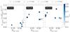 |
Fig. 13. Efstathiou-Lake-Negroponte criterion: quantity vc, max/(αMdiscG)1/2, calculated at t = 0, for all thin+thick disc models as a function of maximum bar strength (Sbar, max). Left panels: evolution for the rthickS models, and the middle and right panels show the evolution for models rthickE and rthickG, respectively. The points are colour-coded by the corresponding thick-disc fraction, fthick (see the colour bar). The different symbols represent thin+thick models with different scale heights. The horizontal line (in black) denotes vc, max/(αMdiscG)1/2 = 1.1, which serves as a boundary for the bar instability phase. For details, see the text. |
7. Discussion
7.1. Caveat to our analysis
In what follows, we discuss some of the implications and limitations of this work. First, in the thin+thick models we considered, the stars are separated into two well-defined and distinct populations, namely, thin- and thick-disc stars. We point out that this scheme of segregating stars into two distinct populations might be suitable for external galaxies, which have two discrete disc structures, but this is a simplification for the Milky Way, where stars of different mono-abundance populations smoothly transition from a thin to a thick disc. Bovy et al. (2012) showed that the disc properties vary continuously with the scale height. Treating the stars separated into two distinct populations therefore reduces the complexity that is expected to be present in the Milky Way. Nevertheless, this discretised treatment of stars with a varying fraction of thick disc stars provides valuable insight into the trends that will be followed by the stellar populations in the external disc galaxies. We further mention that some of the findings of this work can be extended to more complex configurations. For example, a similar radial velocity dispersion for the thin and thick disc at the end of the simulation run, as shown here, was also found in Di Matteo et al. (2019), who modelled the galaxy with three components (thin, intermediate, and thick discs).
The radial extents of the thin and thick discs merit some discussion. The extent of the thick disc partially depends on how it is defined. To illustrate this, when the thick disc component for the Milky Way is defined in terms of the α-enhanced stars, the scale length of the thick disc is smaller than that for the thin disc. However, when the classification for the thick disc is based on colours and not the chemical abundances, the thick-disc scale length is larger than that of the thin disc (e.g., see Jurić et al. 2008). In external galaxies, the thick discs are generally also more extended than the thin disc (e.g., see Yoachim & Dalcanton 2006). This motivated us to consider all three possibilities for the thin-to-thick disc scale length ratio (rthickS, rthickE, and rthickG) and to address the bar formation scenario for a wide range of thin- to thick-disc geometry configurations.
Furthermore, the thin+thick models we used are collisionless simulations and do not contain any interstellar gas. The dynamical role of the interstellar gas in the context of the generation/destruction of disc instabilities, such as bars (Bournaud et al. 2005) and spiral arms (Sellwood & Carlberg 1984; Ghosh & Jog 2015, 2016, 2022), has been investigated in the literature. The presence of a (dynamically) cold component, such as gas, makes the disc more susceptible to gravitational instabilities (e.g., see Jog & Solomon 1984; Jog 1996; Bertin 2000). Furthermore, Bournaud et al. (2005) argued that the inflow of the gas into the central region infuses angular momentum, thereby leading to a significant bar weakening. However, recent observational work by Pahwa & Saha (2018) showed prominent bars in several low surface brightness (LSB) galaxies with a high gas fraction. Nevertheless, the bar formation scenario in the presence of the thick disc and the interstellar gas is well worth investigating.
7.2. Formation of bars in thick discs
The simulations analysed in this paper show that a bar can also form in thick-disc-dominated galaxies or in purely thick-disc galaxies for sufficiently compact distributions (in terms of scale lengths and heights). In particular, our models show that a bar could also have formed in thick discs with characteristics similar to those of the α-enhanced thick disc of the Milky Way (scale length of 2 kpc, scale height of 0.9 kpc; see Bovy et al. 2012), even if the thin-disc counterpart were not yet in place. For a galaxy such as the Milky Way, the formation of the thin disc started about 9 Gyr ago (z ∼ 1; see Haywood et al. 2013; Snaith et al. 2014). This suggests that the Milky Way bar may have been forming or been in place already at these epochs. This finding may in principle push (Haywood et al. 2016; Bovy et al. 2019) the time of the bar formation in our Galaxy to earlier epochs than suggested so far, with an upper limit to its formation possibly set by the end of the epoch of significant mergers experienced by the Milky Way, which is currently estimated at about 10 ± 1 Gyr ago (see Belokurov et al. 2018; Di Matteo et al. 2019; Kruijssen et al. 2020). As discussed previously, it would be crucial to investigate how the inclusion of gas in the models can modify these suggestions. Furthermore, recent observations of rest-frame near-infrared images with the JWST clearly showed prominent bars in disc galaxies in the high-redshift universe (z > 1) as well (Guo et al. 2023). In these redshift ranges, the disc galaxies are thought to be clumpy, turbulent, and more importantly, to have thick discs (e.g., see Hamilton-Campos et al. 2023). The results presented here clearly demonstrated that bar formation in the presence of thick discs is possible even when the thick-disc stars dominate the underlying mass distribution. Therefore, our study here provides a natural explanation for the bar formation scenario in high-redshift galaxies, as recently unveiled by the JWST observations.
7.3. Criteria for the bar formation
As shown earlier, the OP criterion fails to predict the bar formation scenario correctly for some cases, especially for the thick-disc-only models with larger scale heights. However, this is expected because the OP criterion does not include all the complexity related to the bar formation and its growth. For example, the formalism does not take the interaction between the disc and the dark matter halo into account. The limiting value of the ratio of the rotational kinetic energy to the potential energy, W, exceeding 0.14 ± 0.003 in order to become bar stable was derived from simulations with a rigid and not a live dark matter halo (also see the discussion in Athanassoula 2008).
The limited success of the predictability of the ELN criterion for our models is also expected because the ELN criterion was originally developed based on 2D simulation models, and hence it does not take into account the (destabilising) effect of the disc-dark matter halo interaction. Furthermore, it does not take into account the (stabilising) effect of the disc velocity dispersion or the central concentration of the dark matter halo (for details, see the discussions in Athanassoula 2008; Romeo et al. 2023). The recent study of Romeo et al. (2023) showed that for their sample of selected observed galaxies, in only 50−55% of the cases did the ELN criterion successfully predict the bar formation scenario. On the other hand, the study of Izquierdo-Villalba et al. (2022) showed that for about 70−80% of the galaxies taken from the IllustrisTNG simulations, the ELN criterion correctly predicted the bar formation scenario.
8. Summary
In summary, we investigated the dynamical effect of a geometrically thick disc on the bar formation and evolution scenario. We constructed a suite of N-body models of thin+thick discs and systematically varied mass fraction of the thick disc and the different thin-to-thick disc scale length ratios. Our main findings are listed below.
-
Bars form in almost all thin+thick disc models with a varying thick disc mass fraction and for all three geometric configurations with different thin-to-thick disc scale length ratios. The bar is present in both thin- and thick-disc stars. The bar in the thick disc always remains weaker than the bar in the thin-disc stars. Nevertheless, the overall trend of the bar evolution and growth in the thin and thick disc is similar.
-
Bars form quite early (∼2 Gyr) in almost all thin+thick disc models we considered. The models in which the thick-disc scale length is shorter than that of the thin disc (rthickS models) form the bar relatively earlier than in the other two geometry configurations. In addition, the bars in the rthickS models display a more rapid growth in the initial phase than the other two geometry configurations.
-
The bar formation in thick-disc-only simulations (without any thin disc) critically depends on the scale length and scale height of the thick disc. With increasing scale length (and for a fixed scale height), the bar formation epoch is delayed, and the resulting bar is progressively weaker. Similarly, with increasing scale height (and for a fixed scale length), the system becomes progressively hostile to bar formation.
-
The formation of a stronger bar is associated with a higher angular momentum loss and with a more intense radial heating within the bar region, in agreement with previous findings. Moreover, we demonstrated a preferential loss of angular momentum and a preferentially increased radial heating along the 2D extent of the bar. This trend holds true for the thin- and thick-disc stars, and it remains generic for all thin+thick models we considered.
-
We find that the OP criterion is a better prescription than the ELN criterion for predicting bar formation scenarios in our thin+thick models. While the OP criterion almost always correctly predicts the bar instability in our models, the success of predicting the bar instability from the ELN criterion remains only limited for our models.
To conclude, even the inclusion of a massive (kinematically hot) thick-disc component is not efficient in suppressing the bar instability, suggesting that bars can form in hot thick discs at high redshifts. These results agree with recent observational evidence from the JWST, and provide a natural explanation for the bar formation scenario in disc galaxies in the high-redshift universe (z > 1). Our study demonstrated that if the disc galaxy consists only of a thick disc, the bar formation can only be delayed/prevented (within a Hubble time) if the disc scale length is larger (i.e., with less centrally concentrated surface density) and/or if the vertical scale height is larger (i.e., more vertically extended and kinematically hotter) in disc galaxies.
Or equivalently, the mass fraction in the thick disc, because all the disc particles have the same mass.
This is the angular size of a group of distant particles, seen from the particle. If the angular size of the group, seen from the particle, is smaller than θ, then the tree code computes the contribution of the gravitational force (by that group of distant particles) acting on a given particle using the multipole moments of the group mass distribution.
This is basically the specific radial random kinetic energy.
Acknowledgments
We thank the anonymous referee for useful comments which helped to improve this paper. S.G. acknowledges funding from the Alexander von Humboldt Foundation, through Dr. Gregory M. Green’s Sofja Kovalevskaja Award.This work has made use of the computational resources obtained through the DARI grant A0120410154 (P.I.: P. Di Matteo).
References
- Aguerri, J. A. L., Muñoz-Tuñón, C., Varela, A. M., & Prieto, M. 2000, A&A, 361, 841 [NASA ADS] [Google Scholar]
- Aguerri, J. A. L., Méndez-Abreu, J., & Corsini, E. M. 2009, A&A, 495, 491 [NASA ADS] [CrossRef] [EDP Sciences] [Google Scholar]
- Athanassoula, E. 2003, MNRAS, 341, 1179 [Google Scholar]
- Athanassoula, E. 2008, MNRAS, 390, L69 [NASA ADS] [CrossRef] [Google Scholar]
- Athanassoula, E., & Misiriotis, A. 2002, MNRAS, 330, 35 [Google Scholar]
- Athanassoula, E., & Sellwood, J. A. 1986, MNRAS, 221, 213 [Google Scholar]
- Athanassoula, E., Lambert, J. C., & Dehnen, W. 2005, MNRAS, 363, 496 [Google Scholar]
- Athanassoula, E., Machado, R. E. G., & Rodionov, S. A. 2013, MNRAS, 429, 1949 [Google Scholar]
- Aumer, M., & Binney, J. 2017, MNRAS, 470, 2113 [NASA ADS] [CrossRef] [Google Scholar]
- Barnes, J., & Hut, P. 1986, Nature, 324, 446 [NASA ADS] [CrossRef] [Google Scholar]
- Barway, S., Wadadekar, Y., & Kembhavi, A. K. 2011, MNRAS, 410, L18 [NASA ADS] [CrossRef] [Google Scholar]
- Belokurov, V., Erkal, D., Evans, N. W., Koposov, S. E., & Deason, A. J. 2018, MNRAS, 478, 611 [Google Scholar]
- Bertin, G. 2000, Dynamics of Galaxies (Cambridge: Cambridge University Press) [Google Scholar]
- Binney, J., & Tremaine, S. 2008, Galactic Dynamics: Second Edition (Princeton: Princeton University Press) [Google Scholar]
- Bournaud, F., Combes, F., & Semelin, B. 2005, MNRAS, 364, L18 [Google Scholar]
- Bovy, J., Rix, H.-W., Liu, C., et al. 2012, ApJ, 753, 148 [Google Scholar]
- Bovy, J., Rix, H.-W., Schlafly, E. F., et al. 2016, ApJ, 823, 30 [NASA ADS] [CrossRef] [Google Scholar]
- Bovy, J., Leung, H. W., Hunt, J. A. S., et al. 2019, MNRAS, 490, 4740 [Google Scholar]
- Burstein, D. 1979, ApJ, 234, 829 [NASA ADS] [CrossRef] [Google Scholar]
- Buta, R., Laurikainen, E., Salo, H., & Knapen, J. H. 2010, ApJ, 721, 259 [NASA ADS] [CrossRef] [Google Scholar]
- Combes, F., Debbasch, F., Friedli, D., & Pfenniger, D. 1990, A&A, 233, 82 [NASA ADS] [Google Scholar]
- Comerón, S., Elmegreen, B. G., Knapen, J. H., et al. 2011a, ApJ, 741, 28 [CrossRef] [Google Scholar]
- Comerón, S., Knapen, J. H., Sheth, K., et al. 2011b, ApJ, 729, 18 [CrossRef] [Google Scholar]
- Comerón, S., Salo, H., Peletier, R. F., & Mentz, J. 2016, A&A, 593, L6 [NASA ADS] [CrossRef] [EDP Sciences] [Google Scholar]
- Comerón, S., Salo, H., & Knapen, J. H. 2018, A&A, 610, A5 [NASA ADS] [CrossRef] [EDP Sciences] [Google Scholar]
- Comerón, S., Salo, H., Knapen, J. H., & Peletier, R. F. 2019, A&A, 623, A89 [NASA ADS] [CrossRef] [EDP Sciences] [Google Scholar]
- Contopoulos, G., & Grosbol, P. 1989, A&ARv, 1, 261 [Google Scholar]
- Debattista, V. P., & Sellwood, J. A. 1998, ApJ, 493, L5 [Google Scholar]
- Debattista, V. P., & Sellwood, J. A. 2000, ApJ, 543, 704 [Google Scholar]
- Debattista, V. P., Ness, M., Gonzalez, O. A., et al. 2017, MNRAS, 469, 1587 [Google Scholar]
- Di Matteo, P., Fragkoudi, F., Khoperskov, S., et al. 2019, A&A, 628, A11 [NASA ADS] [CrossRef] [EDP Sciences] [Google Scholar]
- Dubinski, J., Berentzen, I., & Shlosman, I. 2009, ApJ, 697, 293 [NASA ADS] [CrossRef] [Google Scholar]
- Efstathiou, G., Lake, G., & Negroponte, J. 1982, MNRAS, 199, 1069 [NASA ADS] [CrossRef] [Google Scholar]
- Elmegreen, B. G., Elmegreen, D. M., & Hirst, A. C. 2004, ApJ, 612, 191 [NASA ADS] [CrossRef] [Google Scholar]
- Eskridge, P. B., Frogel, J. A., Pogge, R. W., et al. 2000, AJ, 119, 536 [NASA ADS] [CrossRef] [Google Scholar]
- Fragkoudi, F., Di Matteo, P., Haywood, M., et al. 2017, A&A, 606, A47 [NASA ADS] [CrossRef] [EDP Sciences] [Google Scholar]
- Fragkoudi, F., Grand, R. J. J., Pakmor, R., et al. 2020, MNRAS, 494, 5936 [Google Scholar]
- Fragkoudi, F., Grand, R. J. J., Pakmor, R., et al. 2021, A&A, 650, L16 [NASA ADS] [CrossRef] [EDP Sciences] [Google Scholar]
- Ghosh, S., & Jog, C. J. 2015, MNRAS, 451, 1350 [NASA ADS] [CrossRef] [Google Scholar]
- Ghosh, S., & Jog, C. J. 2016, MNRAS, 459, 4057 [NASA ADS] [CrossRef] [Google Scholar]
- Ghosh, S., & Jog, C. J. 2018, A&A, 617, A47 [NASA ADS] [CrossRef] [EDP Sciences] [Google Scholar]
- Ghosh, S., & Jog, C. J. 2022, A&A, 658, A171 [NASA ADS] [CrossRef] [EDP Sciences] [Google Scholar]
- Ghosh, S., Saha, K., Di Matteo, P., & Combes, F. 2021, MNRAS, 502, 3085 [NASA ADS] [CrossRef] [Google Scholar]
- Gilmore, G., & Reid, N. 1983, MNRAS, 202, 1025 [Google Scholar]
- Grand, R. J. J., Springel, V., Gómez, F. A., et al. 2016, MNRAS, 459, 199 [Google Scholar]
- Guo, Y., Jogee, S., Finkelstein, S. L., et al. 2023, ApJ, 945, L10 [NASA ADS] [CrossRef] [Google Scholar]
- Hamilton-Campos, K. A., Simons, R. C., Peeples, M. S., Snyder, G. F., & Heckman, T. M. 2023, ApJ, submitted [arXiv:2303.04171] [Google Scholar]
- Haywood, M., Di Matteo, P., Lehnert, M. D., Katz, D., & Gómez, A. 2013, A&A, 560, A109 [NASA ADS] [CrossRef] [EDP Sciences] [Google Scholar]
- Haywood, M., Di Matteo, P., Snaith, O., & Calamida, A. 2016, A&A, 593, A82 [NASA ADS] [CrossRef] [EDP Sciences] [Google Scholar]
- Hernquist, L., & Weinberg, M. D. 1992, ApJ, 400, 80 [Google Scholar]
- Hohl, F. 1971, ApJ, 168, 343 [NASA ADS] [CrossRef] [Google Scholar]
- Hozumi, S., & Hernquist, L. 2005, PASJ, 57, 719 [NASA ADS] [CrossRef] [Google Scholar]
- Izquierdo-Villalba, D., Bonoli, S., Rosas-Guevara, Y., et al. 2022, MNRAS, 514, 1006 [NASA ADS] [CrossRef] [Google Scholar]
- Jean-Baptiste, I., Di Matteo, P., Haywood, M., et al. 2017, A&A, 604, A106 [NASA ADS] [CrossRef] [EDP Sciences] [Google Scholar]
- Jog, C. J. 1996, MNRAS, 278, 209 [NASA ADS] [CrossRef] [Google Scholar]
- Jog, C. J., & Solomon, P. M. 1984, ApJ, 276, 114 [NASA ADS] [CrossRef] [Google Scholar]
- Jogee, S., Barazza, F. D., Rix, H.-W., et al. 2004, ApJ, 615, L105 [NASA ADS] [CrossRef] [Google Scholar]
- Jurić, M., Ivezić, Ž., Brooks, A., et al. 2008, ApJ, 673, 864 [Google Scholar]
- Kasparova, A. V., Katkov, I. Y., Chilingarian, I. V., et al. 2016, MNRAS, 460, L89 [NASA ADS] [CrossRef] [Google Scholar]
- Kim, T., Sheth, K., Gadotti, D. A., et al. 2015, ApJ, 799, 99 [NASA ADS] [CrossRef] [Google Scholar]
- Klypin, A., Valenzuela, O., Colín, P., & Quinn, T. 2009, MNRAS, 398, 1027 [Google Scholar]
- Kraljic, K., Bournaud, F., & Martig, M. 2012, ApJ, 757, 60 [Google Scholar]
- Kruijssen, J. M. D., Pfeffer, J. L., Chevance, M., et al. 2020, MNRAS, 498, 2472 [NASA ADS] [CrossRef] [Google Scholar]
- Kruk, S. J., Lintott, C. J., Simmons, B. D., et al. 2017, MNRAS, 469, 3363 [NASA ADS] [CrossRef] [Google Scholar]
- Martig, M., Pinna, F., Falcón-Barroso, J., et al. 2021, MNRAS, 508, 2458 [NASA ADS] [CrossRef] [Google Scholar]
- Martinez-Valpuesta, I., Shlosman, I., & Heller, C. 2006, ApJ, 637, 214 [NASA ADS] [CrossRef] [Google Scholar]
- Masters, K. L., Nichol, R. C., Hoyle, B., et al. 2011, MNRAS, 411, 2026 [Google Scholar]
- Melvin, T., Masters, K., Lintott, C., et al. 2014, MNRAS, 438, 2882 [Google Scholar]
- Mihos, J. C., McGaugh, S. S., & de Blok, W. J. G. 1997, ApJ, 477, L79 [NASA ADS] [CrossRef] [Google Scholar]
- Miyamoto, M., & Nagai, R. 1975, PASJ, 27, 533 [NASA ADS] [Google Scholar]
- Nair, P. B., & Abraham, R. G. 2010, ApJ, 714, L260 [Google Scholar]
- Ohta, K., Hamabe, M., & Wakamatsu, K.-I. 1990, ApJ, 357, 71 [Google Scholar]
- Ostriker, J. P., & Peebles, P. J. E. 1973, ApJ, 186, 467 [Google Scholar]
- Pahwa, I., & Saha, K. 2018, MNRAS, 478, 4657 [NASA ADS] [CrossRef] [Google Scholar]
- Pfenniger, D., & Norman, C. 1990, ApJ, 363, 391 [Google Scholar]
- Pinna, F., Falcón-Barroso, J., Martig, M., et al. 2018, MNRAS, 475, 2697 [NASA ADS] [CrossRef] [Google Scholar]
- Pinna, F., Falcón-Barroso, J., Martig, M., et al. 2019a, A&A, 623, A19 [NASA ADS] [CrossRef] [EDP Sciences] [Google Scholar]
- Pinna, F., Falcón-Barroso, J., Martig, M., et al. 2019b, A&A, 625, A95 [NASA ADS] [CrossRef] [EDP Sciences] [Google Scholar]
- Plummer, H. C. 1911, MNRAS, 71, 460 [Google Scholar]
- Pohlen, M., Balcells, M., Lütticke, R., & Dettmar, R. J. 2004, A&A, 422, 465 [NASA ADS] [CrossRef] [EDP Sciences] [Google Scholar]
- Press, W. H., Flannery, B. P., & Teukolsky, S. A. 1986, Numerical Recipes. The Art of Scientific Computing (Cambridge: Cambridge University Press) [Google Scholar]
- Rodionov, S. A., Athanassoula, E., & Sotnikova, N. Y. 2009, MNRAS, 392, 904 [NASA ADS] [CrossRef] [Google Scholar]
- Romeo, A. B., Agertz, O., & Renaud, F. 2023, MNRAS, 518, 1002 [Google Scholar]
- Rosas-Guevara, Y., Bonoli, S., Dotti, M., et al. 2022, MNRAS, 512, 5339 [NASA ADS] [CrossRef] [Google Scholar]
- Saha, K. 2014, ArXiv e-prints [arXiv:1403.1711] [Google Scholar]
- Saha, K., & Elmegreen, B. 2018, ApJ, 858, 24 [NASA ADS] [CrossRef] [Google Scholar]
- Saha, K., & Naab, T. 2013, MNRAS, 434, 1287 [NASA ADS] [CrossRef] [Google Scholar]
- Saha, K., Tseng, Y.-H., & Taam, R. E. 2010, ApJ, 721, 1878 [Google Scholar]
- Saha, K., Graham, A. W., & Rodríguez-Herranz, I. 2018, ApJ, 852, 133 [NASA ADS] [CrossRef] [Google Scholar]
- Scott, N., van de Sande, J., Sharma, S., et al. 2021, ApJ, 913, L11 [NASA ADS] [CrossRef] [Google Scholar]
- Sellwood, J. A., & Carlberg, R. G. 1984, ApJ, 282, 61 [Google Scholar]
- Sellwood, J. A., & Debattista, V. P. 2006, ApJ, 639, 868 [NASA ADS] [CrossRef] [Google Scholar]
- Semelin, B., & Combes, F. 2002, A&A, 388, 826 [NASA ADS] [CrossRef] [EDP Sciences] [Google Scholar]
- Shen, J., & Sellwood, J. A. 2004, ApJ, 604, 614 [NASA ADS] [CrossRef] [Google Scholar]
- Sheth, K., Elmegreen, D. M., Elmegreen, B. G., et al. 2008, ApJ, 675, 1141 [Google Scholar]
- Simmons, B. D., Melvin, T., Lintott, C., et al. 2014, MNRAS, 445, 3466 [NASA ADS] [CrossRef] [Google Scholar]
- Snaith, O. N., Haywood, M., Di Matteo, P., et al. 2014, ApJ, 781, L31 [CrossRef] [Google Scholar]
- Snaith, O., Haywood, M., Di Matteo, P., et al. 2015, A&A, 578, A87 [NASA ADS] [CrossRef] [EDP Sciences] [Google Scholar]
- Toomre, A. 1964, ApJ, 139, 1217 [Google Scholar]
- Tremaine, S., & Weinberg, M. D. 1984, MNRAS, 209, 729 [Google Scholar]
- Tsikoudi, V. 1979, ApJ, 234, 842 [NASA ADS] [CrossRef] [Google Scholar]
- van der Kruit, P. C., & Freeman, K. C. 2011, ARA&A, 49, 301 [Google Scholar]
- Vieira, K., Carraro, G., Korchagin, V., et al. 2022, ApJ, 932, 28 [NASA ADS] [CrossRef] [Google Scholar]
- Vynatheya, P., Saha, K., & Ghosh, S. 2021, MNRAS, submitted [arXiv:2105.03183] [Google Scholar]
- Whyte, L. F., Abraham, R. G., Merrifield, M. R., et al. 2002, MNRAS, 336, 1281 [NASA ADS] [CrossRef] [Google Scholar]
- Wozniak, H., & Pierce, M. J. 1991, A&AS, 88, 325 [NASA ADS] [Google Scholar]
- Wozniak, H., Friedli, D., Martinet, L., Martin, P., & Bratschi, P. 1995, A&AS, 111, 115 [NASA ADS] [Google Scholar]
- Yoachim, P., & Dalcanton, J. J. 2006, AJ, 131, 226 [NASA ADS] [CrossRef] [Google Scholar]
Appendix A: Rbar measurement for the thin+thick models
In the literature, both observationally and from simulations, a wide variety of techniques has been employed to measure the bar length, Rbar. This includes isophotal fitting with an ellipse (e.g., Wozniak & Pierce 1991; Wozniak et al. 1995), a Fourier analysis of the azimuthal luminosity profiles (e.g., Ohta et al. 1990), measuring the location of the maximum of the bar– inter-bar luminosity ratio (Aguerri et al. 2000), finding the deviation in the phase angle by a certain amount (5 − 10°), and by measuring the location in which the A2/A0 (m = 2 Fourier coefficient) drops to a certain fraction of its peak value.
We briefly describe how we calculated the Rbar in our thin+thick disc models. To achieve this, we used two methods. In the first method, we defined Rbar as the location in which the A2/A0 value drops to 60% of its peak value. In the second method, we defined the Rbar as the location in which the A2/A0 value drops to 70% of its peak value. The corresponding temporal evolution of Rbar, calculated for the total (thin+thick) disc particles, is shown in Fig. A.1 for model rthickE0.5. The values of Rbar clearly increase quite significantly, by almost a factor of about two. However, after about 6 Gyr, the bar does not grow appreciably, and the values of Rbar also saturate, with occasional fluctuations (compare Figs. 3 and A.1). Therefore, we took this value as the representative value for Rbar (see the horizontal magenta line in Fig. A.1). The Rbar values for all other thin+thick disc models were determined in this fashion, and they are indicated in Fig. 1 (see the dashed black circles there).
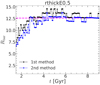 |
Fig. A.1. Temporal evolution of the bar length, Rbar, measured by the two methods we adopted (see the text for details) for model rthickE0.5. The horizontal magenta line denotes the representative value for the Rbar we used for this model. |
All Tables
All Figures
|
Fig. 1. Face-on density distribution of all disc particles (thin+thick) at the end of the simulation run (t = 9 Gyr) for all thin+thick disc models with varying fthick values. The white solid lines denote the constant density contours. The solid black circle in each sub-panel denotes the corresponding extent of the bar (Rbar). Left panels: density distribution for the rthickS models, and the middle and right panels: density distribution for the rthickE and rthickG models, respectively. The thick disc fraction (fthick) varies from 0.1 to 1 (top to bottom), as indicated in the left-most panel of each row. A prominent bar forms in almost all models considered here. |
| In the text | |
|
Fig. 2. Radial profiles of the m = 2, 4, 6 Fourier coefficients (normalised by the m = 0 component), for the thin disc (left panels), thick-disc stars (middle panels), and total (thin+thick) disc stars (right panels) as a function of time (shown in the colour bar) for the model rthickE0.5. At later times, the peaks of the radial profiles of the m = 2, 4, 6 Fourier coefficients shift towards the outer regions. |
| In the text | |
|
Fig. 3. Temporal evolution of the bar strength, Sbar, for the thin-disc (upper panels), thick-disc (middle panels), and total (thin+thick) disc stars (lower panels) for all thin+thick disc models with varying fthick values (see the colour bar). Left panels: bar strength evolution for the rthickS models, and the middle and right panels: evolution of the bar strength for the rthickE and rthickG models, respectively. The thick-disc fraction (fthick) varies from 0.1 to 0.9 (with a step size of 0.2), as indicated in the colour bar. The solid blue lines in the bottom row denote the three thick-disc-only models (fthick = 1), and the solid red line in the top middle panel denotes the thin-disc-only model (fthick = 0). For details see text. |
| In the text | |
|
Fig. 4. Temporal evolution of the growth/decay rate of the bar strength (dSbar/dt), for the thin-, thick-, and total (thin+thick) disc components for all models with varying fthick values. Left panels: evolution for the rthickS models, and the middle and right panels: evolution for the rthickE and rthickG models, respectively. The fthick values are indicated in the left-most panel of each row. Top middle row: growth/decay rate of the bar strength for the thin-disc-only model (fthick = 0). |
| In the text | |
|
Fig. 5. Temporal evolution of the bar strength Sbar for the six thick-disc-only models with a varying vertical scale height. For details, see the text. The solid line denotes the rthickE models, the dashed line denotes the rthickG models, and the dotted line denotes the rthickS models. Different line colours denote models with different scale-height values. With increasing vertical scale height, the models progressively become bar stable. The horizontal line denotes Sbar = 0.2 and is used as a (operational) limit for the onset of bar formation. |
| In the text | |
|
Fig. 6. Temporal evolution of the z-component of the specific angular momentum, calculated within the extent of the bar, lz(t; R < Rbar) (see Eq. (5)), for the thin- (in blue), thick- (in red), and total (thin+thick) disc (in black) particles for all thin+thick disc models. For each model, Rbar was first fixed to a saturation/representative value. For details, see Sect. 5.1. Left panels: evolution for the rthickS models, and the middle and right panels: evolution for the rthickE and rthickG models, respectively. The thick-disc fraction (fthick) varies from 0.1 to 1 (top to bottom), as indicated in the left-most panel of each row. The extents of bars in each sub-panel are as indicated in Fig. 1 (see the solid black circles there). |
| In the text | |
|
Fig. 7. Distribution of the z-component of the specific angular momentum in the face-on projection ((x, y)-plane) at different times for the thin- (left panels), thick- (middle panels), and thin+thick disc particles (right panels) for the model rthickE0.5. The dotted lines denote the contours of the total (thin+thick) surface density. The dashed black circle in each sub-panel denotes the extent of the bar. |
| In the text | |
|
Fig. 8. Temporal evolution of the average radial random kinetic energy, calculated within the extent of the bar, ⟨ΠR(t; R < Rbar)⟩ (see Eq. (7)), for the thin- (in blue), thick- (in red), and total (thin+thick) disc (in black) particles for all thin+thick disc models. For each model, Rbar was first fixed to a saturation/representative value. For details, see Sect. 5.1. Left panels: evolution for the rthickS models, and the middle and right panels: evolution for models rthickE and rthickG, respectively. The value of fthick varies from 0.1 to 1 (top to bottom), as indicated in the left-most panel of each row. The extents of the bars in each sub-panel are indicated in Fig. 1 (see the solid black circles there). |
| In the text | |
|
Fig. 9. Distribution of the change in the average radial random kinetic energy, Δ⟨ΠR⟩(x, y, t) (see Eq. (8)), calculated in the face-on projection ((x, y)-plane) at different times for the thin- (left panels), thick- (middle panels), and thin+thick disc particles (right panels) for model rthickE0.5. The dotted lines denote the contours of the total (thin+thick) surface density. The dashed black circle in each sub-panel denotes the extent of the bar. |
| In the text | |
|
Fig. 10. Distribution of the change in average radial random kinetic energy and the specific angular momentum for the total (thin+thick) disc within the bar region (see Eqs. (9) and (10)) for all models considered here. Left panels: evolution for the rthickS models, and the middle and right panels: evolution for the rthickE and rthickG models, respectively. The points are colour-coded by the maximum value of the bar strength (Sbar, max). The increasing size of the points denotes a higher thick-disc fraction (fthick = 0.1 − 1). |
| In the text | |
|
Fig. 11. Ostriker-Peeble (OP) criterion: ratio of the total mean kinetic energy to the total random kinetic energy, calculated within the extent of the bar, (Π/Tmean(t; R < Rbar)), at t = 0 for the total (thin+thick) disc as a function of the maximum bar strength (Sbar, max). Left panels: evolution for the rthickS models, and the middle and right panels: evolution for models rthickE and rthickG, respectively. The points are colour-coded by the corresponding thick-disc fraction, fthick (see the colour bar). Different symbols represent thin+thick models with different scale heights. For details, see the text. The shaded region denotes the bar-stable zone according to the OP criterion. |
| In the text | |
|
Fig. 12. Evolution of the ratio of the total mean kinetic energy to total random kinetic energy, calculated within the extent of the bar, (Π/Tmean(t; R < Rbar)), for the total (thin+thick) disc particles, plotted against the growth rate of the bar (dSbar/dt) for all thin+thick models with varying fthick values. Left panels: evolution for the rthickS models, and the middle and right panels: evolution for models rthickE and rthickG, respectively. The thick-disc fraction (fthick) varies from 0.1 to 1 (top to bottom), as indicated in the left-most panel of each row. The points are colour-coded by the simulation time (see the colour bar). The vertical black line denotes Π/Tmean = 5.14, which serves as a boundary for the bar instability phase, and the grey shaded region (in each sub-panel) denotes the bar-stable phase according to the OP criterion. For details, see the text. |
| In the text | |
|
Fig. 13. Efstathiou-Lake-Negroponte criterion: quantity vc, max/(αMdiscG)1/2, calculated at t = 0, for all thin+thick disc models as a function of maximum bar strength (Sbar, max). Left panels: evolution for the rthickS models, and the middle and right panels show the evolution for models rthickE and rthickG, respectively. The points are colour-coded by the corresponding thick-disc fraction, fthick (see the colour bar). The different symbols represent thin+thick models with different scale heights. The horizontal line (in black) denotes vc, max/(αMdiscG)1/2 = 1.1, which serves as a boundary for the bar instability phase. For details, see the text. |
| In the text | |
|
Fig. A.1. Temporal evolution of the bar length, Rbar, measured by the two methods we adopted (see the text for details) for model rthickE0.5. The horizontal magenta line denotes the representative value for the Rbar we used for this model. |
| In the text | |
Current usage metrics show cumulative count of Article Views (full-text article views including HTML views, PDF and ePub downloads, according to the available data) and Abstracts Views on Vision4Press platform.
Data correspond to usage on the plateform after 2015. The current usage metrics is available 48-96 hours after online publication and is updated daily on week days.
Initial download of the metrics may take a while.