| Issue |
A&A
Volume 683, March 2024
|
|
|---|---|---|
| Article Number | A238 | |
| Number of page(s) | 17 | |
| Section | Extragalactic astronomy | |
| DOI | https://doi.org/10.1051/0004-6361/202347099 | |
| Published online | 22 March 2024 | |
JADES: The emergence and evolution of Lyα emission and constraints on the intergalactic medium neutral fraction⋆
1
Department of Physics, University of Oxford, Denys Wilkinson Building, Keble Road, Oxford OX1 3RH, UK
e-mail: This email address is being protected from spambots. You need JavaScript enabled to view it.
2
Department of Physics and Astronomy, University College London, Gower Street, London WC1E 6BT, UK
3
Kavli Institute for Cosmology, University of Cambridge, Madingley Road, Cambridge CB3 0HA, UK
4
Cavendish Laboratory, University of Cambridge, 19 JJ Thomson Avenue, Cambridge CB3 0HE, UK
5
Steward Observatory, University of Arizona, 933 N. Cherry Ave., Tucson, AZ 85721, USA
6
Centro de Astrobiología (CAB), CSIC–INTA, Cra. de Ajalvir Km. 4, 28850 Torrejón de Ardoz, Madrid, Spain
7
European Space Agency (ESA), European Space Astronomy Centre (ESAC), Camino Bajo del Castillo s/n, 28692 Villanueva de la Cañada, Madrid, Spain
8
European Space Agency, ESA/ESTEC, Keplerlaan 1, 2201 AZ Noordwijk, The Netherlands
9
Jodrell Bank Centre for Astrophysics, Department of Physics and Astronomy, School of Natural Sciences, The University of Manchester, Manchester M13 9PL, UK
10
School of Physics, University of Melbourne, Parkville, 3010 VIC, Australia
11
ARC Centre of Excellence for All Sky Astrophysics in 3 Dimensions (ASTRO 3D), Stromlo, ACT 2611, Australia
12
Scuola Normale Superiore, Piazza dei Cavalieri 7, 56126 Pisa, Italy
13
Sorbonne Université, CNRS, UMR 7095, Institut d’Astrophysique de Paris, 98 bis bd Arago, 75014 Paris, France
14
European Southern Observatory, Karl-Schwarzschild-Strasse 2, 85748 Garching, Germany
15
Centre for Astrophysics Research, Department of Physics, Astronomy and Mathematics, University of Hertfordshire, Hatfield AL10 9AB, UK
16
Center for Astrophysics | Harvard & Smithsonian, 60 Garden St., Cambridge, MA 02138, USA
17
Department of Physics and Astronomy, The Johns Hopkins University, 3400 N. Charles St., Baltimore, MD 21218, USA
18
AURA for European Space Agency, Space Telescope Science Institute, 3700 San Martin Drive, Baltimore, MD 21210, USA
19
Department of Astronomy, University of Wisconsin-Madison, 475 N. Charter St., Madison, WI 53706, USA
20
Max-Planck-Institut für Astronomie, Königstuhl 17, 69117 Heidelberg, Germany
21
Department of Astronomy and Astrophysics, University of California, Santa Cruz, 1156 High Street, Santa Cruz, CA 95064, USA
22
Astrophysics Research Institute, Liverpool John Moores University, 146 Brownlow Hill, Liverpool L3 5RF, UK
23
NSF’s National Optical-Infrared Astronomy Research Laboratory, 950 North Cherry Avenue, Tucson, AZ 85719, USA
24
NRC Herzberg, 5071 West Saanich Rd, Victoria, BC V9E 2E7, Canada
Received:
5
June
2023
Accepted:
20
December
2023
Abstract
The rest-frame UV recombination emission line Lyα can be powered by ionising photons from young massive stars in star-forming galaxies, but the fact that it can be resonantly scattered by neutral gas complicates its interpretation. For reionisation-era galaxies, a neutral intergalactic medium will scatter Lyα from the line of sight, making Lyα a useful probe of the neutral fraction evolution. Here, we explore Lyα in JWST/NIRSpec spectra from the ongoing JADES programme, which targets hundreds of galaxies in the well-studied GOODS-S and GOODS-N fields. These sources are UV-faint (−20.4 < MUV < −16.4) and thus represent a poorly explored class of galaxy. We fitted the low spectral resolution spectra (R ∼ 100) of a subset of 84 galaxies in GOODS-S with zspec > 5.6 (as derived with optical lines) with line and continuum models to search for significant line emission. Through exploration of the R100 data, we find evidence for Lyα in 17 sources. This sample allowed us to place observational constraints on the fraction of galaxies with Lyα emission in the redshift range 5.6 < z < 7.5, with a decrease from z = 6 to z = 7. We also find a positive correlation between the Lyα equivalent width and MUV, as seen in other samples. We used these results to estimate the neutral gas fraction at z ∼ 7, and our estimates are in agreement with previous results (XHI ∼ 0.5 − 0.9).
Key words: galaxies: high-redshift / intergalactic medium / dark ages / reionization / first stars
Comparison sample is available at the CDS via anonymous ftp to cdsarc.cds.unistra.fr (130.79.128.5) or via https://cdsarc.cds.unistra.fr/viz-bin/cat/J/A+A/683/A238
© The Authors 2024
 Open Access article, published by EDP Sciences, under the terms of the Creative Commons Attribution License (https://creativecommons.org/licenses/by/4.0), which permits unrestricted use, distribution, and reproduction in any medium, provided the original work is properly cited.
This article is published in open access under the Subscribe to Open model. This email address is being protected from spambots. You need JavaScript enabled to view it. to support open access publication.
1. Introduction
By studying the properties of galaxies at high redshifts (such as morphology, spectral energy distributions, and kinematics), we are able to chart how populations of galaxies have evolved through cosmic time. In individual galaxies we can study the buildup of gaseous reservoirs, the conversion of this fuel into stars, and the effects of feedback. By studying the overall galaxy population as a function of redshift, we can determine the evolution of the luminosity function, the star formation rate density, and the growth of supermassive black holes. In parallel, these studies shine light on the last great phase transition of the Universe, when the intergalactic medium (IGM) became ionised: the epoch of reionisation (EoR).
This epoch began at the end of the “cosmic dark ages”, when the first stars formed (e.g. Villanueva-Domingo et al. 2018). The UV radiation of these objects created ionised regions (i.e. “bubbles”), which grew and merged together (e.g. Gnedin 2000). Observations suggest that the IGM was mostly ionised at z ∼ 6 (tH ∼ 0.91 Gyr; e.g. Fan et al. 2006), although the details of reionisation are still being derived (e.g. the drivers; Hutchison et al. 2019; Naidu et al. 2020; Endsley et al. 2021, topology; Pentericci et al. 2014; Larson et al. 2022; Yoshioka et al. 2022, and timeline; Christenson et al. 2021; Cain et al. 2021; Zhu et al. 2022). One of the most useful tools for studying this epoch is the bright Lyman-α line of hydrogen (λ = 1215.67 Å; hereafter Lyα).
As the lowest-energy transition (n = 2 → 1) of the most abundant element, Lyα emission should be ubiquitous. But this radiation can be absorbed and re-radiated by any other hydrogen atom in the ground state (i.e. HI). For galaxies at z ≲ 6, this repeated absorption and re-radiation by neutral gas inside a galaxy (i.e. resonant scattering) means that Lyα can be greatly reduced in intensity but also observed along sight lines far from the original emission region, as seen in large Lyα halos of ∼10 kpc (e.g. Drake et al. 2022; Kikuta et al. 2023) or ∼100 kpc (e.g. Steidel et al. 2000; Reuland et al. 2003; Dey et al. 2005; Cai et al. 2017; Li et al. 2021; Guo et al. 2023; Zhang et al. 2024).
For galaxies in the EoR, neutral gas in the IGM surrounding a galaxy can also scatter Lyα emission, resulting in a lower observed brightness (e.g. Fontana et al. 2010; Stark et al. 2010). In order for this emission to be observable, it must lie in an ionised bubble (e.g. Mason & Gronke 2020) and/or feature a significant outflow (e.g. Dijkstra & Wyithe 2010). So by comparing the fraction of galaxies with Lyα emission to the expected number from models (Lyα fraction; XLyα), we are able to place constraints on the HI filling fraction (XHI; e.g. Ono et al. 2012; Mason et al. 2018; Matthee et al. 2022).
Constraints on XLyα have been placed for galaxies from 4 ≲ z ≲ 8 (e.g. Stark et al. 2011, 2017; Curtis-Lake et al. 2012; Caruana et al. 2012, 2014; Ono et al. 2012; Schenker et al. 2014; Pentericci et al. 2018; Yoshioka et al. 2022) and down to z ∼ 2 (e.g. Cassata et al. 2015). By comparing the observed evolution of XLyα to that expected from different Lyα luminosity functions, some works have placed constraints on XHI, suggesting that it quickly decreased from ≳0.9 to ∼0 between z ∼ 8 and z ∼ 6 (e.g. Mason et al. 2018, 2019; Morales et al. 2021). Therefore, the study of galaxies in this short time interval (∼0.3 Gyr) is key to characterising the timeline of reionisation. While a number of studies have been undertaken, observations have been hampered by small sample sizes, limited volumes (prone to cosmic variance), or a focus on bright (MUV ≲ −20) or strongly lensed sources (e.g. Hoag et al. 2019; Fuller et al. 2020; Bolan et al. 2022). Already, the James Webb Space Telescope (JWST) Near-Infrared Spectrograph (NIRSpec; Jakobsen et al. 2022; Böker et al. 2023) has seen great success in detecting Lyα (e.g. Bunker et al. 2023b; Jung et al. 2023; Roy et al. 2023; Tang et al. 2023). But to reduce sample variance and allow stronger conclusions, a wide-area survey down to MUV ∼ −18.75 is needed (e.g. Taylor & Lidz 2014). With JWST, such a survey is possible.
The JWST Advance Deep Extragalactic Survey (JADES; Bunker et al. 2020; Eisenstein et al. 2023) is a cycle 1−2 guaranteed time observation (GTO) programme for observing the Great Observatories Origins Deep Survey (GOODS; Dickinson et al. 2003) north (N) and south (S) fields. It uses JWST/NIRSpec in multi-object spectroscopy mode (Ferruit et al. 2022) in both low spectral resolution (R100) and medium spectral resolution (R1000), in combination with the JWST/Near-Infrared Camera (NIRCam; Rieke et al. 2023).
This rich dataset is the subject of numerous ongoing investigations, including detailed modelling of the Lyα profiles using the R1000 spectra (e.g. asymmetry and velocity offsets; Saxena et al. 2024), analysis of the damping wings (Jakobsen et al., in prep.), and a search for Lyα overdensities that hint at large ionised bubbles (Witstok et al. 2024). In this work, we search for Lyα emission in the R100 spectra of data from GOODS-S for the purpose of placing constraints on the neutral gas fraction at z ∼ 6 − 8. These fits are used to examine correlations between the Lyα rest-frame equivalent width (REWLyα), redshift, and UV absolute magnitude.
We describe our sample in Sect. 2. The details and results of our R100 spectral fitting procedure are given in Sect. 3. These findings are discussed in Sect. 4, and we conclude in Sect. 5. We assume a standard concordance cosmology throughout: (ΩΛ, Ωm, h) = (0.7, 0.3, 0.7).
2. Sample
2.1. Observation overview
JADES consists of two survey depths: “Deep” and “Medium”. The former allows for the characterisation of a small number of dimmer galaxies or more detailed study of individual sources at higher S/N, while the latter enables a statistical characterisation of the galaxy population at high-z. In addition, each tier has two stages with different selections: one based on existing Hubble Space Telescope (HST) imaging (followed by “/HST”) and the other based on JWST/NIRCam imaging (followed by “/JWST”; see Eisenstein et al. 2023 for more details).
From the JADES survey, we utilised data from galaxies in GOODS-S in the Deep/HST (PID: 1210, PI: N. Lützgendorf), Medium/HST (PID: 1180, PI: D. Eisenstein), and Medium/JWST (PID: 1286, PI: N. Lützgendorf) sub-surveys. Target catalogues were created for each tier, with galaxies assigned priority classes based on photometric redshift, apparent UV-brightness, and visual inspection of existing ancillary data (for more details on Deep/HST priority classes, see Bunker et al. 2023a). Galaxies with zphot > 5.6 were collected from studies that selected sources based on the Lyman-break drop out selection (e.g. Bunker et al. 2004; Bouwens et al. 2015; Harikane et al. 2016), or Lyman-break galaxies (LBGs). This system ensures that both rare (e.g. bright, high-redshift, hosts of active galactic nuclei) and representative systems would be observed. Due to the geometrical constraints dictated by mask construction, galaxies were randomly selected for observation from each priority class.
Details of the data acquisition and reduction details are given in other works (Curtis-Lake et al. 2023; Carniani et al. 2024), which we summarise here. Targets were observed with three shutters in a three-point nod. In order to improve data quality, sub-pointings were created for each primary pointing by shifting the JWST/NIRSpec Multi-Shutter Array (MSA) by a few shutters in each direction. Due to failed shutters, not all targets were observable in all three sub-pointings. This results in exposure times of sources in R100 for Deep/HST of 33.6−100.8 ks for 253 observed sources. Medium/JWST features a similar setup, but with a lower R100 exposure time per target: 5.3−8.0 ks for 169 observed sources. While 1354 galaxies were observed in Medium/HST, the majority of the executions (8/12) were negatively affected by a short circuit in the MSA, making the data unusable. The mean exposure time for R100 per object of the usable data is 3.8 ks (Eisenstein et al. 2023). Observations were repeated for some of these objects with unusable data (364 sources), with a mean R100 exposure time per object of 7.5 − 11.3 ks.
The resulting raw data were calibrated using a pipeline developed by the European Space Agency (ESA) NIRSpec Science Operations Team (SOT) and the NIRSpec GTO Team, which includes corrections for outlier rejection (e.g. “snowballs”), background subtraction (using adjacent slits), wavelength grid resampling, and slit loss. This results in two-dimensional spectra with data quality flags, which were used to extract a one-dimensional spectrum and a noise spectrum.
2.2. Sample construction
The resulting spectra of all observed sources were visually inspected and strong emission lines (e.g. [OIII]λ5007, Hα) were fit. We imposed a lower redshift limit of zspec > 5.6 in order to ensure a sample of LBGs. This yielded a sample of 84 galaxies at z ≳ 5.6 (38 from Medium/HST, 13 from Medium/JWST, and 33 from Deep/HST) with precise spectroscopic redshifts (full details in Bunker et al. 2023a). Both R100 and R1000 spectra are available for these galaxies, and we used the R100 spectra in this work1.
Our sample of 84 galaxies is composed of galaxies at zspec > 5.6 (i.e. LBGs) with cuts on UV brightness in HST broadband filters redwards of the Lyman break. Some sources were excluded from our sample for a lack of strong emission lines (i.e. a poorly constrained zspec). While this results in a more complex sample than the uniform sample selection of some previous studies (e.g. Pentericci et al. 2018; Yoshioka et al. 2022), this inhomogeneity is taken into account through the error spectrum of each source and a completeness analysis.
3. Combined Lyα and continuum fit
At these high redshifts, the spectra exhibit a strong continuum break at the Lyα wavelength at the redshift of the galaxy. The deep sensitivity of the R100 data allows us to simultaneously characterise any Lyα emission and the underlying continuum of each source. To do this, we examined whether a two-component model (i.e. line and continuum) or a single-component model (i.e. only continuum) better fits the extracted spectrum of each source using LMFIT (Newville et al. 2014). This process is detailed below.
3.1. Resolution effects
Due to the low spectral resolution of the R100 data, we had to consider both the wavelength grid and spectral dispersion. The spectral pixels in our calibrated data are large (Δv ∼ 2000 − 2600 km s−1 per pixel at the redshifted Lyα wavelength for galaxies at z ∼ 5.6 − 10). Furthermore, for galaxies observed in the EoR this wavelength is near the minimum of the PRISM resolving power curve2, with R ∼ 30. This implies that the line-spread function (LSF) has a full width at half maximum of ∼104 km s−1. Although for a compact source that does not fill the slit, the resolving power will in practice be higher by as much as a factor of 2 (de Graaff et al. 2024).
The low resolution also makes it impossible to characterise the Lyα profile (e.g. asymmetry, velocity offset). Instead, the Lyα emission can be approximated as additional flux in the first spectral bin redwards of the Lyα break, which is spread into neighbouring bins by the LSF.
To demonstrate how this affects the interpretation of R100 spectra, we first created a higher-resolution (Δλ = 0.001 μm, or R ∼ 730) model of a Lyα break (modelled as a step function) at z = 7 with no Lyα flux (blue line in the top panel of Fig. 1). If we account for the LSF by convolving the spectrum with a Gaussian (σR = λLyα/R/2.355), the break becomes an S-shaped curve instead (orange histogram). Rebinning this curve to the coarser R100 wavelength grid maintains the curve, but at lower resolution (green histogram).
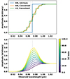 |
Fig. 1. Demonstration of how Lyα break and emission for a source at z = 7 are affected by the low resolving power of our observations. The top panel shows how a step function (blue line) is affected by the resolving power on a high-resolution (Δλ = 0.001 μm) spectral grid (orange curve), and how this curve would appear on the R100 spectral grid (green steps). If we add Lyα emission with a given REWLyα in the first high-resolution spectral bin redwards of the break and then account for the LSF and R100 spectral bin, we find the curves in the lower panel. |
If we add Lyα flux with a given REWLyα to the intrinsic high-resolution model as additional flux in the first spectral bin redwards of the Lyα break, convolve the model with the LSF, and re-bin the result to the R100 spectral grid, we find the profiles shown in the lower panel of Fig. 1. The line flux is spread from one low-resolution pixel into a Gaussian that spans both sides of the Lyα break. Even high-REWLyα lines (e.g. 100 Å) have low peaks (here 4× the continuum level). In addition, low-REWLyα lines (< 20 Å) feature very low amplitudes, and instead appear similar to a pure continuum model with a blueshifted Lyα break.
With this in mind, our model fitting procedure begins with a high-resolution spectral model, which is convolved with a Gaussian to account for the resolving power and then rebinned to the R100 spectral grid. This allows us to compare the observed and model spectra directly, in order to extract the intrinsic continuum and Lyα flux.
3.2. Model description
We first assumed that the underlying continuum can be approximated by a power law and used a Heaviside step function to represent the Lyα break (see Appendix B for a discussion of this assumption). This continuum-only model only features two variables: the continuum value at a rest-frame wavelength of 1500 Å (SC, o) and the spectral slope just redwards of Lyα (n; ∼1300 − 1500 Å rest-frame), which is not fixed to the redder (i.e. ∼1400 − 2300 Å rest-frame) spectral slope β derived by Saxena et al. (2024).
In the case where both continuum and Lyα emission are detected, the line emission will have a REW of
 (1)
(1)
where FLyα is the total line flux of Lyα. As discussed in Sect. 3.1, the low spectral resolution of the R100 data dictates that our line emission model is simple. Our combined line and continuum model thus has three variables: those of the continuum model (i.e. SC, o and n) and REWLyα.
For both the continuum and line+continuum models, we first created a spectral grid of high resolution (Δλ = 0.001 μm) and populated each bin using a continuum-only or continuum and line model. As discussed in Sect. 3.1, we then convolved the spectrum with a Gaussian that accounts for the LSF. We first considered using a Gaussian based on the theoretical resolving power as recorded in the JWST documentation (σR = λLyα/R/2.355). However, this was calculated assuming a source that illuminates the slit uniformly, which is not the case for the relatively compact sources in our sample. Detailed LSFs for the sources in Deep/HST have been calculated (de Graaff et al. 2024), which reveal that the actual LSF is smaller than the theoretical value, by a factor of up to ∼2.4. However these models are not available for our whole sample. To account for the LSF in a uniform manner, we convolved the model spectrum with a Gaussian of width FRσR, where FR is allowed to vary. These data were then re-binned to the R100 spectral grid of an observation.
3.3. Fitting procedure
We used LMFIT with a “leastsq” minimiser to fit each convolved model to a subset of the observed spectrum. Each data point was weighted by its associated inverse variance (as derived from the error spectrum).
We limited the fit subset to the wavelength range [(λLyα±(0.03 μm))×(1+z)], with a minimum of ≥0.75 μm. This range was chosen to avoid including excessive amounts of noisy data at blue wavelengths below the Lyα break, and to only fit the continuum just redwards of Lyα, avoiding nearby emission lines (e.g. [CIV]λλ1548, 1551 and HeIIλ1640).
While precise systemic redshifts for each source have been derived using fits to strong lines (e.g. [OIII]λ5007 and Hα) using the higher spectral resolution gratings (Bunker et al. 2023a), it is possible that the Lyα emission is shifted into a neighbouring spectral bin by a large velocity offset (i.e. up to a few hundred km s−1; Erb et al. 2014; Marchi et al. 2019) or a different binning scheme between the gratings and prism. This is accounted for by allowing the redshift of Lyα emission to vary from the systemic redshift within the R100 bin, taking the result with the lowest χ2.
Next, we considered the lowest REW line that we can detect for each source. Because the line emission is spread from one into multiple channels by convolution with the LSF, we could approximate the 1σ limit on REWLyα in the R100 spectrum as
 (2)
(2)
where FRσR is the width of the LSF and E(λ) is the error spectrum.
The results of the continuum (“C”) and line and continuum (“L+C”) are examined, and a definite Lyα detection is reported if both of the following criteria are met:
-
The “L+C” fit features a lower
 than the “C” fit.
 -
The best-fit REWLyα is greater than 2.5ΔREWLyα, 1σ.
When Lyα is detected, we take the best-fit REWLyα value and its associated uncertainty from our fit. Otherwise, we treat the Lyα line as undetected, and use 3ΔREWLyα, 1σ as an upper limit.
3.4. Results
With this definition, we find that 17 galaxies in our sample feature significant Lyα emission from the R100 spectra alone. The best-fit models of these detections are shown in Figs. 2 and A.1 while the best-fit parameters of all galaxies in our sample are presented in Appendix C.
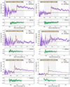 |
Fig. 2. Results of fitting a line plus continuum model to observed JADES R100 data, for sources detected in Lyα emission (denoted by “L+C FIT”). In each top panel, we show the observed spectrum (purple line) with an associated 1σ error (shaded region). The best-fit model, which includes the effects of the LSF, is shown by a yellow line. Fitting was performed using the wavelength range that is shaded grey. The continuum value at the redshifted Lyα wavelength is represented by a brown star. The bottom panel shows the residual. Continued in Fig. A.1. |
For comparison, we present REWLyα values derived by taking the continuum values from this work and the Lyα fluxes measured from the R1000 spectra by Saxena et al. (2024). These line fluxes were only measured for galaxies at z > 5.8 in the Deep/HST and Medium/HST tiers in GOODS-S (excluding Medium/JWST, where there are no z > 5.8 galaxies detected in Lyα emission). For some of these sources, Lyα fell into the unobservable chip gap, so no Lyα is given.
We note that the use of the low spectral resolution PRISM/CLEAR grating/filter combination (R ∼ 100) results in detections or limits that are in agreement (i.e. within 3σ) with the higher-resolution R1000 data for every source. This is encouraging, as the latter is more sensitive to low equivalent width lines. For example, Bunker et al. (2023b) find that Lyα is not observable in the R100 spectrum of GNz-11, but is clearly detected in the R1000 spectrum. This can also be seen in our sources that are undetected in the prism, but have a 3σ REWLyα, R100 upper limit that agrees with a smaller REWLyα, R1000 value (i.e. our REWLyα upper limit from the prism is consistent with the value of the REWLyα inferred from the grating detection).
From our R100 fitting analysis, we find that 17 of the 84 galaxies in our sample are detected in Lyα. In the following subsections, we analyse the properties of these detections.
3.5. Completeness analysis
As seen in Eq. (2), our REW sensitivity is dependent on observational parameters (error spectrum and LSF) as well as source properties (redshift and continuum flux). To further complicate matters, the error spectrum features higher values at small wavelengths, resulting in larger uncertainties in E(λLyα, obs) for lower redshift sources. Our sample is quite diverse in redshift, continuum strength (i.e. MUV), and sensitivity (i.e. Deep and Medium tiers). So while Eq. (2) can be used as a limit on REW, it does not capture the breadth of galaxy properties in our sample, and an estimation of the completeness of our sample is required (e.g. Thai et al. 2023).
To begin, we assumed a similar model to the previous subsections: a power-law continuum, a Lyα break given by a Heaviside step function, and Lyα emission quantified as an REW. The mean uncertainty spectra for each tier were calculated by averaging the corresponding error spectra. For each galaxy, we took the best-fit continuum strength (MUV) and redshift (z), and created 50 mock spectra by sampling from uniform distributions of β = [ − 2.5, 2.5], and FR = [0.1, 0.8]. This process was repeated for three REW values (25 Å, 50 Å, and 75 Å). Gaussian noise was added based on the error spectrum. Each of these 12 900 model spectra was fit with the procedure outlined in Sect. 3.3, and the completeness for each galaxy and REW value was then estimated as the fraction of models that are well fit (i.e. that return a REW value within 3σ of the input value).
This analysis yields an average completeness for our sample of C25 Å = 0.33, C50 Å = 0.60, and C75 Å = 0.74. As expected, the completeness of each tier increases with REW. Our completeness at REW = 25 Å is low, which results in poor constraints on XLyα and XHI (see Sects. 4.3 and 4.4). We use these completeness values to derive corrected Lyα fractions in the next section.
4. Discussion
4.1. Source properties
To demonstrate the multi-tier complexity of our sample, we show the systemic redshift (based on the identification of rest-frame optical lines; Bunker et al. 2023a) and the 1500 Å continuum magnitude (hereafter MUV), separated by survey tier (Fig. 3). Previous studies defined UV-faint galaxies as those with MUV > −20.25 (e.g. Curtis-Lake et al. 2012), which shows that most of the JADES sample contains faint sources. The high-redshift bins (z > 8) are dominated by the Deep/HST sources, but the 5.6 < z < 7.5 regime is well explored by all three subsamples. The overall sample is well sampled in the MUV ∼ −19.5 to −17.5 regime, but extends down to MUV ∼ −16.5.
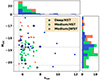 |
Fig. 3. MUV (from NIRSpec spectra; see Appendix D) versus systemic redshift (based on optical lines) for our sample. Galaxies observed in different tiers are coloured differently. Sources detected in Lyα emission are shown as diamonds with black outlines. Horizontal dashed lines show MUV values of −18.75 and −20.25, while the vertical grey line shows our lower redshift cutoff (zsys > 5.6). |
The sources with Lyα detections in R100 data are contained within z ∼ 5.6 − 8.0, and span a wide range of MUV ∼ −20.5 to −17. Of the 51 sources in the Medium tiers, 7 are detected in Lyα (∼ 14%). On the other hand, 10 of the 33 Deep galaxies are Lyα-detected (∼30%). In the next subsection, we explore the limits that the non-detections imply.
4.2. Equivalent width–UV magnitude relation
A recent analysis of JWST/NIRSpec MSA data from the Cosmic Evolution Early Release Science (CEERS) survey (Tang et al. 2023) and data at lower redshift showed a positive correlation between REWLyα and MUV for a sample of galaxies with high O32 values (i.e. a high level of ionisation). To investigate this relation further, we first collected a literature sample of galaxies with reported spatial positions, spectroscopic redshifts, REWLyα from spectral observations, and MUV values (including that of Tang et al. 2023; see Appendix E) and split this sample into different redshift bins (Fig. 4).
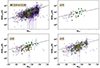 |
Fig. 4. Distribution of Lyα REWs as a function of MUV for our sample (orange circles for detections and green triangles for 3σ upper limits) and from the literature (purple circles for detections and red triangles for 3σ upper limits). An illustrative fit to the detections is shown by the black dashed line. See Appendix E for details of the literature sample. |
In each redshift bin, there appears to be a positive correlation between REWLyα and MUV, such that UV-fainter (higher MUV) objects feature higher Lyα equivalent widths. To illustrate this, we fitted a simple model to the data, which resulted in positive slopes (see the dashed black line). We do not present the fit values or uncertainty, as the literature sample is not constructed with a single set of criteria.
While this trend may be physical, it may also be influenced by the sensitivity limits of observations. As a test of this, we created a set of simulated R100 spectra that do not feature any relation between REW and MUV, fitted them with our method, and plotted the resulting best-fit values and upper limits (see Appendix F). This test shows that we are not able to recover UV-faint, low-REW galaxies, resulting in an apparent positive correlation. While this does not affect the conclusion of other works, we cannot claim a correlation based on our data.
4.3. Lyα fraction
Next, we derived the fraction of galaxies in our sample that are detected in Lyα emission (XLyα). This has been a focus of multiple studies over the past decade (e.g. Stark et al. 2011, 2017; Curtis-Lake et al. 2012; Ono et al. 2012; Caruana et al. 2012, 2014; Schenker et al. 2014; Pentericci et al. 2018; Yoshioka et al. 2022), where subsamples are usually created according to cuts on MUV and the value of REWLyα.
The most well-studied sample for XLyα evolution is that of galaxies with −21.75 < MUV < −20.25 and REWLyα > 25 Å (e.g. Fontana et al. 2010; Stark et al. 2011, 2017; Ono et al. 2012; Curtis-Lake et al. 2012; Schenker et al. 2012, 2014; Pentericci et al. 2014, 2018; Cassata et al. 2015; Yoshioka et al. 2022). For these galaxies, studies have hinted at a steep increase in XLyα between z = 7 and 6, with a shallower drop off between z = 6 − 4. Since the JADES sample contains fainter galaxies (see Fig. 3), we were instead able to focus on fainter galaxies (MUV > −20.25).
We first divided our sample of galaxies into discrete redshift bins and calculated effective sample sizes by summing their completeness values (Sect. 3.5). The Lyα fraction was then found by dividing the number of galaxies in the redshift bin that meet the REW limit by the effective sample size (e.g. Caruana et al. 2012). This was repeated for three cuts on REWLyα (> 25 Å, > 50 Å, or > 75 Å), and we compared them to observed fractions from the literature for galaxies fainter than MUV > −20.25 (Stark et al. 2010, 2011; Ono et al. 2012; Schenker et al. 2012, 2014; Pentericci et al. 2014, 2018; see Fig. 5).
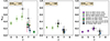 |
Fig. 5. Fraction of observed galaxies detected in Lyα emission with REWLyα > 25 Å (left), REWLyα > 50 Å (centre), and REWLyα > 75 Å (right). Derived fractions from the literature are shown by coloured markers. For the central panel, note that Stark et al. (2011) and Ono et al. (2012) used a REW limit of > 55 Å. The fractions derived using only the observed JADES galaxies are shown by black points. Our REW > 25 Å values (grey) are likely affected by low completeness. |
For galaxies with −20.25 < MUV < −18.75, previous studies have shown that the fraction for EW > 25 Å increases from z = 7 to z = 6 with evidence for a decrease to z = 4, presumably due to the onset of IGM neutrality. Due to the low completeness of our sample at 25 Å (see Sect. 3.5), we are not able to place tight constraints on XLyα in this REW regime. Despite this, our estimates are in agreement with previous findings. The higher completeness at REW > 50 Å and REW > 75 Å results in agreement with previous results.
Overall, our sample supports a rise in the Lyα fraction between z = 7 and z = 6, as seen in previous studies. Since JADES is ongoing, future investigations will include more data and yield tighter constraints on the evolution of this quantity. Even with our current data, we are able to constrain the IGM neutral fraction, as seen in the next subsection.
4.4. Constraints on the neutral fraction
The observed Lyα fraction of galaxies for a given redshift, MUV bin, and REWLyα limit provides valuable information on the neutral fraction of the IGM (XHI). This is due to the fact that the evolution of XLyα(z ≲ 6) is dependent only on galaxy properties, while at z ≳ 6 it is also dependent on the properties of IGM transmission. Some studies compared observed XLyα(z ∼ 7) with the fraction expected from simulations, resulting in a range of estimates for XHI(z = 7): ≲0.3 (Stark et al. 2010), ∼0.5 (Caruana et al. 2014), ≳0.51 (Pentericci et al. 2014), ∼0.6 − 0.9 (Ono et al. 2012), ≲0.7 (Furusawa et al. 2016). This discrepancy may be partially explained by sample properties (e.g. difference in MUV ranges and small sample sizes).
The conversion from XLyα to XHI is non-trivial, and is dependent on the simulation used for comparison to observations. For example, the semi-numerical code DexM (Mesinger & Furlanetto 2007; Mesinger et al. 2011; Zahn et al. 2011) has been used by some works (e.g. Dijkstra et al. 2011; Pentericci et al. 2014) to create three-dimensional models of galaxy halos, determine how they ionise their surroundings, and characterise their redshift evolution. The outputs of this process (e.g. XLyα) can then be compared to observations.
While an updated simulation is beyond the scope of this work, we can use our XLyα(REWLyα) values at z ∼ 7 to generate a cumulative distribution function (CDF) of REWLyα, and compare this to model outputs of Pentericci et al. (2014). This model is appropriate for galaxies with −20.25 < MUV < −18.75 and assumes NHI = 1020 cm−2 and a wind speed of 200 km s−1, but with a variable neutral fraction. It is based on the assumption that the Lyα CDF at z = 6 and z = 7 are intrinsically the same, but are observed to differ because of neutral IGM attenuation at z = 7. As seen in Fig. 6, higher values of XHI result in less Lyα transmission, and thus a steeper CDF. Literature values (Ono et al. 2012; Schenker et al. 2012; Pentericci et al. 2014, 2018) appear to argue for a value of XHI ∼ 0.5 − 0.9.
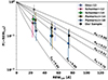 |
Fig. 6. Cumulative distribution for Lyα REW for UV-faint galaxies (−20.25 < MUV < −18.75) at z ∼ 7. Each solid line shows the expected distribution for a model with NHI = 1020 cm−2 and a wind speed of 200 km s−1, but with a different neutral fraction (Pentericci et al. 2014). Estimates from the literature (Ono et al. 2012; Schenker et al. 2012, 2014; Pentericci et al. 2014, 2018) are shifted by 1 Å for visibility. Our P(REW > 25 Å) point (grey) is likely affected by low completeness. |
Our results (using a wide redshift bin of 6 < z < 8) are in agreement with those of the previous studies (e.g. Mason et al. 2018), suggesting an approximate XHI of ∼0.2 − 0.7. We note that our P(REW > 25 Å) point is influenced by poor completeness, and thus does not provide a constraint. We note that this MUV range is not optimised for our sample, and a future work will investigate how the redshift evolution (z = 8 − 6) of P(> REW) for −20.4 < MUV < −16 galaxies can be used to constrain XHI(z).
The XHI range of our analysis agrees with previous analyses that use the REWLyα cumulative distribution (e.g. Schenker et al. 2014; Pentericci et al. 2014, 2018) as well as simulations (e.g. Mason et al. 2018). This suggests that our estimates of P(> REW) have not been underestimated due to the NIRSpec MSA shutters (0.2″ ∼ 1 kpc at z ∼ 7) missing Lyα flux from extended halos, as noted by Jung et al. (2023). In this previous study, FLyα, MSA for one observed source was only 20% of the value derived using the Multi-Object Spectrometer for Infra-Red Exploration (MOSFIRE) instrument on the Keck I telescope. On the other hand, Tang et al. (2023) found agreement between MSA- and ground-based estimates of FLyα for four z ∼ 7 − 9 galaxies (but with large uncertainties for two sources). In addition, large Lyα halos are commonly seen at low-z, but will not have time to evolve for high-redshift sources. So while slit losses are unlikely to affect our results, this effect can be further investigated by observing representative sources with the NIRSpec Integral Field Unit (IFU; field of view of 3″ × 3″), or forward modelling the slit losses in simulations.
5. Conclusions
In this work we present the first constraints on Lyα emission using JWST/NIRSpec MSA R100 spectra from the JADES survey. The increased sensitivity of this instrument enables deeper investigations of faint galaxies in the early Universe. Our sample consists of 84 galaxies at z > 5.6, each with secure spectroscopic redshifts (Bunker et al. 2023a). While the sample is concentrated at 5.6 ≲ z ≲ 7.5, we included sources up to z ∼ 12. In addition, the MUV ∼ −19.5 to −17.5 range is well probed, but we included sources that are fainter (MUV ∼ −16) and brighter (MUV ∼ −20.4).
By fitting each spectrum with a line and/or continuum model, accounting for the spectral dispersion, and comparing the relative goodness-of-fit values, we find that 17 sources at z ∼ 5.6 − 8.0 show evidence for Lyα emission in R100. The strong continuum of each source enabled us to estimate the continuum flux (and MUV) at the Lyα wavelength directly from the spectra. We derived Lyα REWs for each source.
We built a large comparison sample from the literature of galaxies with estimates of spectroscopic redshifts, MUV, and REWLyα. By combining the JADES and literature samples, we find that the reported positive correlation between MUV and REWLyα is supported for galaxies in multiple redshift bins, but the observed correlation in our data may be caused by sensitivity effects.
Next, we calculated the redshift evolution of the Lyα fraction (XLyα) in bins of REWLyα. Due to the faintness of the JADES sample (MUV ≳ −20.4), we were able to place constraints on the poorly studied faint, high-redshift (z ∼ 6 − 7) evolution of this fraction: a shallow increase from z = 7 to z = 6 for REW > 50 Å and REW > 75 Å.
The distribution of REWLyα values was then used to place a constraint on the neutral fraction (XHI) at z ∼ 7 using the Pentericci et al. (2014) model. Our results indicate XHI ∼ 0.2 − 0.7, which is in agreement with previous studies.
The JADES survey is still ongoing, so this dataset will expand with time. In addition, many sources feature higher-resolution R1000 spectra, which enable further science cases such as Lyα velocity offset and line asymmetry analysis, damping wing modelling, and environments of Lyα emitters (LAEs). Combined, these analyses will reveal the details of reionisation in unprecedented detail.
Details of the R1000 analysis are presented in an associated paper (Saxena et al. 2024).
As recorded in the JWST documentation: https://jwst-docs.stsci.edu/jwst-near-infrared-spectrograph/nirspec-instrumentation/nirspec-dispersers-and-filters
A full machine readable table of the comparison sample is available in electronic form at the CDS.
Acknowledgments
G.C.J., A.J.B., A.S., A.J.C., and J.C. acknowledge funding from the “FirstGalaxies” Advanced Grant from the European Research Council (ERC) under the European Union’s Horizon 2020 research and innovation programme (Grant agreement No. 789056). J.W., R.M., W.M.B., T.J.L., L.S., and J.S. acknowledge support by the Science and Technology Facilities Council (STFC) and by the ERC through Advanced Grant 695671 “QUENCH”. J.W. also acknowledges funding from the Fondation MERAC. R.M. also acknowledges funding from the UKRI Frontier Research grant RISEandFALL and from a research professorship from the Royal Society. S.A. acknowledges support from Grant PID2021-127718NB-I00 funded by the Spanish Ministry of Science and Innovation/State Agency of Research (MICIN/AEI/ 10.13039/501100011033). R.B. acknowledges support from an STFC Ernest Rutherford Fellowship (ST/T003596/1). This research is supported in part by the Australian Research Council Centre of Excellence for All Sky Astrophysics in 3 Dimensions (ASTRO 3D), through project number CE170100013. S.C. acknowledges support by European Union’s HE ERC Starting Grant No. 101040227 – WINGS. E.C.L. acknowledges support of an STFC Webb Fellowship (ST/W001438/1). D.J.E., B.D.J., and B.E.R. acknowledge a JWST/NIRCam contract to the University of Arizona NAS5-02015. D.J.E. is supported as a Simons Investigator. Funding for this research was provided by the Johns Hopkins University, Institute for Data Intensive Engineering and Science (IDIES). R.S. acknowledges support from a STFC Ernest Rutherford Fellowship (ST/S004831/1). H.Ü. gratefully acknowledges support by the Isaac Newton Trust and by the Kavli Foundation through a Newton-Kavli Junior Fellowship. The research of CCW is supported by NOIRLab, which is managed by the Association of Universities for Research in Astronomy (AURA) under a cooperative agreement with the National Science Foundation. G.C.J. would like to thank C. Witten and N. Laporte for valuable insight into the sample. We thank the anonymous referee for constructive feedback that has enhanced this work.
References
- Böker, T., Beck, T. L., Birkmann, S. M., et al. 2023, PASP, 135, 038001 [CrossRef] [Google Scholar]
- Bolan, P., Lemaux, B. C., Mason, C., et al. 2022, MNRAS, 517, 3263 [Google Scholar]
- Bouwens, R. J., Illingworth, G. D., Oesch, P. A., et al. 2015, ApJ, 803, 34 [Google Scholar]
- Bunker, A. J., Stanway, E. R., Ellis, R. S., & McMahon, R. G. 2004, MNRAS, 355, 374 [NASA ADS] [CrossRef] [Google Scholar]
- Bunker, A. J., NIRSPEC Instrument Science Team,& JAESs Collaboration 2020, in Uncovering Early Galaxy Evolution in the ALMA and JWST Era, eds. E. da Cunha, J. Hodge, J. Afonso, L. Pentericci, & D. Sobral, 352, 342 [NASA ADS] [Google Scholar]
- Bunker, A. J., Cameron, A. J., Curtis-Lake, E., et al. 2023a, A&A, submitted [arXiv:2306.02467] [Google Scholar]
- Bunker, A. J., Saxena, A., Cameron, A. J., et al. 2023b, A&A, 677, A88 [NASA ADS] [CrossRef] [EDP Sciences] [Google Scholar]
- Cai, Z., Fan, X., Yang, Y., et al. 2017, ApJ, 837, 71 [NASA ADS] [CrossRef] [Google Scholar]
- Cain, C., D’Aloisio, A., Gangolli, N., & Becker, G. D. 2021, ApJ, 917, L37 [NASA ADS] [CrossRef] [Google Scholar]
- Carniani, S., Venturi, G., Parlanti, E., et al. 2024, A&A, in press, https://doi.org/10.1051/0004-6361/202347230 [Google Scholar]
- Caruana, J., Bunker, A. J., Wilkins, S. M., et al. 2012, MNRAS, 427, 3055 [NASA ADS] [CrossRef] [Google Scholar]
- Caruana, J., Bunker, A. J., Wilkins, S. M., et al. 2014, MNRAS, 443, 2831 [NASA ADS] [CrossRef] [Google Scholar]
- Cassata, P., Tasca, L. A. M., Le Fèvre, O., et al. 2015, A&A, 573, A24 [NASA ADS] [CrossRef] [EDP Sciences] [Google Scholar]
- Christenson, H. M., Becker, G. D., Furlanetto, S. R., et al. 2021, ApJ, 923, 87 [NASA ADS] [CrossRef] [Google Scholar]
- Cuby, J. G., Le Fèvre, O., McCracken, H., et al. 2003, A&A, 405, L19 [NASA ADS] [CrossRef] [EDP Sciences] [Google Scholar]
- Curtis-Lake, E., McLure, R. J., Pearce, H. J., et al. 2012, MNRAS, 422, 1425 [NASA ADS] [CrossRef] [Google Scholar]
- Curtis-Lake, E., Carniani, S., Cameron, A., et al. 2023, Nat. Astron., 7, 622 [NASA ADS] [CrossRef] [Google Scholar]
- de Graaff, A., Rix, H.-W., Carniani, S., et al. 2024, A&A, in press, https://doi.org/10.1051/0004-6361/202347755 [NASA ADS] [CrossRef] [EDP Sciences] [Google Scholar]
- Dey, A., Bian, C., Soifer, B. T., et al. 2005, ApJ, 629, 654 [NASA ADS] [CrossRef] [Google Scholar]
- Dickinson, M., Giavalisco, M., & GOODS Team 2003, in The Mass of Galaxies at Low and High Redshift, eds. R. Bender, & A. Renzini, 324 [Google Scholar]
- Dijkstra, M., & Wyithe, J. S. B. 2010, MNRAS, 408, 352 [NASA ADS] [CrossRef] [Google Scholar]
- Dijkstra, M., Mesinger, A., & Wyithe, J. S. B. 2011, MNRAS, 414, 2139 [NASA ADS] [CrossRef] [Google Scholar]
- Drake, A. B., Neeleman, M., Venemans, B. P., et al. 2022, ApJ, 929, 86 [NASA ADS] [CrossRef] [Google Scholar]
- Eisenstein, D. J., Willott, C., Alberts, S., et al. 2023, ApJS, submitted [arXiv:2306.02465] [Google Scholar]
- Endsley, R., Stark, D. P., Chevallard, J., & Charlot, S. 2021, MNRAS, 500, 5229 [Google Scholar]
- Endsley, R., Stark, D. P., Bouwens, R. J., et al. 2022, MNRAS, 517, 5642 [NASA ADS] [CrossRef] [Google Scholar]
- Erb, D. K., Steidel, C. C., Trainor, R. F., et al. 2014, ApJ, 795, 33 [Google Scholar]
- Fan, X., Strauss, M. A., Becker, R. H., et al. 2006, AJ, 132, 117 [NASA ADS] [CrossRef] [Google Scholar]
- Fan, X., Bañados, E., & Simcoe, R. A. 2023, ARA&A, 61, 373 [NASA ADS] [CrossRef] [Google Scholar]
- Ferruit, P., Jakobsen, P., Giardino, G., et al. 2022, A&A, 661, A81 [NASA ADS] [CrossRef] [EDP Sciences] [Google Scholar]
- Fontana, A., Vanzella, E., Pentericci, L., et al. 2010, ApJ, 725, L205 [Google Scholar]
- Fujimoto, S., Wang, B., Weaver, J., et al. 2023, ApJ, submitted [arXiv:2308.11609] [Google Scholar]
- Fuller, S., Lemaux, B. C., Bradač, M., et al. 2020, ApJ, 896, 156 [NASA ADS] [CrossRef] [Google Scholar]
- Furusawa, H., Kashikawa, N., Kobayashi, M. A. R., et al. 2016, ApJ, 822, 46 [NASA ADS] [CrossRef] [Google Scholar]
- Gnedin, N. Y. 2000, ApJ, 535, 530 [NASA ADS] [CrossRef] [Google Scholar]
- Guo, Y., Bacon, R., Wisotzki, L., et al. 2023, A&A, submitted [arXiv:2309.06311] [Google Scholar]
- Harikane, Y., Ouchi, M., Ono, Y., et al. 2016, ApJ, 821, 123 [NASA ADS] [CrossRef] [Google Scholar]
- Heintz, K. E., Watson, D., Brammer, G., et al. 2023, arXiv e-prints [arXiv:2306.00647] [Google Scholar]
- Hoag, A., Bradač, M., Huang, K., et al. 2019, ApJ, 878, 12 [NASA ADS] [CrossRef] [Google Scholar]
- Hutchison, T. A., Papovich, C., Finkelstein, S. L., et al. 2019, ApJ, 879, 70 [NASA ADS] [CrossRef] [Google Scholar]
- Iye, M., Ota, K., Kashikawa, N., et al. 2006, Nature, 443, 186 [NASA ADS] [CrossRef] [Google Scholar]
- Jakobsen, P., Ferruit, P., Alves de Oliveira, C., et al. 2022, A&A, 661, A80 [NASA ADS] [CrossRef] [EDP Sciences] [Google Scholar]
- Jung, I., Finkelstein, S. L., Larson, R. L., et al. 2022, ApJ, submitted [arXiv:2212.09850] [Google Scholar]
- Jung, I., Finkelstein, S. L., Arrabal Haro, P., et al. 2023, ApJ, submitted [arXiv:2304.05385] [Google Scholar]
- Kerutt, J., Wisotzki, L., Verhamme, A., et al. 2022, A&A, 659, A183 [NASA ADS] [CrossRef] [EDP Sciences] [Google Scholar]
- Kikuta, S., Matsuda, Y., Inoue, S., et al. 2023, ApJ, 947, 75 [NASA ADS] [CrossRef] [Google Scholar]
- Larson, R. L., Finkelstein, S. L., Hutchison, T. A., et al. 2022, ApJ, 930, 104 [NASA ADS] [CrossRef] [Google Scholar]
- Li, J., Emonts, B. H. C., Cai, Z., et al. 2021, ApJ, 922, L29 [NASA ADS] [CrossRef] [Google Scholar]
- Marchi, F., Pentericci, L., Guaita, L., et al. 2019, A&A, 631, A19 [NASA ADS] [CrossRef] [EDP Sciences] [Google Scholar]
- Mason, C. A., & Gronke, M. 2020, MNRAS, 499, 1395 [Google Scholar]
- Mason, C. A., Treu, T., Dijkstra, M., et al. 2018, ApJ, 856, 2 [Google Scholar]
- Mason, C. A., Fontana, A., Treu, T., et al. 2019, MNRAS, 485, 3947 [NASA ADS] [CrossRef] [Google Scholar]
- Matthee, J., Sobral, D., Boogaard, L. A., et al. 2019, ApJ, 881, 124 [NASA ADS] [CrossRef] [Google Scholar]
- Matthee, J., Naidu, R. P., Pezzulli, G., et al. 2022, MNRAS, 512, 5960 [NASA ADS] [CrossRef] [Google Scholar]
- Mesinger, A., & Furlanetto, S. 2007, ApJ, 669, 663 [Google Scholar]
- Mesinger, A., & Furlanetto, S. R. 2008, MNRAS, 385, 1348 [NASA ADS] [CrossRef] [Google Scholar]
- Mesinger, A., Furlanetto, S., & Cen, R. 2011, MNRAS, 411, 955 [Google Scholar]
- Miralda-Escudé, J. 1998, ApJ, 501, 15 [CrossRef] [Google Scholar]
- Morales, A. M., Mason, C. A., Bruton, S., et al. 2021, ApJ, 919, 120 [CrossRef] [Google Scholar]
- Mortlock, D. 2016, Astrophys. Space Sci. Lib., 423, 187 [NASA ADS] [CrossRef] [Google Scholar]
- Naidu, R. P., Tacchella, S., Mason, C. A., et al. 2020, ApJ, 892, 109 [NASA ADS] [CrossRef] [Google Scholar]
- Newville, M., Stensitzki, T., Allen, D. B., et al. 2014, Astrophysics Source Code Library [record ascl:1606.014] [Google Scholar]
- Oesch, P. A., van Dokkum, P. G., Illingworth, G. D., et al. 2015, ApJ, 804, L30 [Google Scholar]
- Oke, J. B., & Gunn, J. E. 1983, ApJ, 266, 713 [NASA ADS] [CrossRef] [Google Scholar]
- Ono, Y., Ouchi, M., Mobasher, B., et al. 2012, ApJ, 744, 83 [Google Scholar]
- Pentericci, L., Vanzella, E., Fontana, A., et al. 2014, ApJ, 793, 113 [NASA ADS] [CrossRef] [Google Scholar]
- Pentericci, L., Vanzella, E., Castellano, M., et al. 2018, A&A, 619, A147 [NASA ADS] [CrossRef] [EDP Sciences] [Google Scholar]
- Prieto-Lyon, G., Mason, C., Mascia, S., et al. 2023, ApJ, 956, 136 [NASA ADS] [CrossRef] [Google Scholar]
- Reuland, M., van Breugel, W., Röttgering, H., et al. 2003, ApJ, 592, 755 [CrossRef] [Google Scholar]
- Richard, J., Claeyssens, A., Lagattuta, D., et al. 2021, A&A, 646, A83 [EDP Sciences] [Google Scholar]
- Rieke, M. J., Kelly, D. M., Misselt, K., et al. 2023, PASP, 135, 028001 [CrossRef] [Google Scholar]
- Roberts-Borsani, G. W., Bouwens, R. J., Oesch, P. A., et al. 2016, ApJ, 823, 143 [NASA ADS] [CrossRef] [Google Scholar]
- Roy, N., Henry, A., Treu, T., et al. 2023, ApJ, 952, L14 [NASA ADS] [CrossRef] [Google Scholar]
- Saxena, A., Bunker, A. J., Jones, G. C., et al. 2024, A&A, in press, https://doi.org/10.1051/0004-6361/202347132 [Google Scholar]
- Schenker, M. A., Stark, D. P., Ellis, R. S., et al. 2012, ApJ, 744, 179 [Google Scholar]
- Schenker, M. A., Ellis, R. S., Konidaris, N. P., & Stark, D. P. 2014, ApJ, 795, 20 [NASA ADS] [CrossRef] [Google Scholar]
- Shibuya, T., Ouchi, M., Harikane, Y., et al. 2018, PASJ, 70, S15 [Google Scholar]
- Song, M., Finkelstein, S. L., Livermore, R. C., et al. 2016, ApJ, 826, 113 [NASA ADS] [CrossRef] [Google Scholar]
- Stark, D. P., Ellis, R. S., Chiu, K., Ouchi, M., & Bunker, A. 2010, MNRAS, 408, 1628 [Google Scholar]
- Stark, D. P., Ellis, R. S., & Ouchi, M. 2011, ApJ, 728, L2 [Google Scholar]
- Stark, D. P., Ellis, R. S., Charlot, S., et al. 2017, MNRAS, 464, 469 [NASA ADS] [CrossRef] [Google Scholar]
- Steidel, C. C., Adelberger, K. L., Shapley, A. E., et al. 2000, ApJ, 532, 170 [NASA ADS] [CrossRef] [Google Scholar]
- Tang, M., Stark, D. P., Chen, Z., et al. 2023, MNRAS, 526, 1657 [NASA ADS] [CrossRef] [Google Scholar]
- Taylor, J., & Lidz, A. 2014, MNRAS, 437, 2542 [NASA ADS] [CrossRef] [Google Scholar]
- Thai, T. T., Tuan-Anh, P., Pello, R., et al. 2023, A&A, 678, A139 [NASA ADS] [CrossRef] [EDP Sciences] [Google Scholar]
- Tilvi, V., Malhotra, S., Rhoads, J. E., et al. 2020, ApJ, 891, L10 [NASA ADS] [CrossRef] [Google Scholar]
- Umeda, H., Ouchi, M., Nakajima, K., et al. 2023, arXiv e-prints [arXiv:2306.00487] [Google Scholar]
- Vanzella, E., Pentericci, L., Fontana, A., et al. 2011, ApJ, 730, L35 [NASA ADS] [CrossRef] [Google Scholar]
- Villanueva-Domingo, P., Gariazzo, S., Gnedin, N. Y., & Mena, O. 2018, JCAP, 2018, 024 [Google Scholar]
- Witstok, J., Smit, R., Saxena, A., et al. 2024, A&A, 682, A40 [NASA ADS] [CrossRef] [EDP Sciences] [Google Scholar]
- Yoshioka, T., Kashikawa, N., Inoue, A. K., et al. 2022, ApJ, 927, 32 [NASA ADS] [CrossRef] [Google Scholar]
- Zahn, O., Mesinger, A., McQuinn, M., et al. 2011, MNRAS, 414, 727 [NASA ADS] [CrossRef] [Google Scholar]
- Zhang, H., Cai, Z., Liang, Y., et al. 2024, ApJ, 961, 63 [NASA ADS] [CrossRef] [Google Scholar]
- Zhu, Y., Becker, G. D., Bosman, S. E. I., et al. 2022, ApJ, 932, 76 [NASA ADS] [CrossRef] [Google Scholar]
- Zitrin, A., Labbé, I., Belli, S., et al. 2015, ApJ, 810, L12 [Google Scholar]
Appendix A: Additional figure
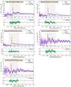 |
Fig. A.1. continued. |
Appendix B: Damping wing in R100
In this work we assumed that the Lyman break can be approximated by a step function. To test whether this is appropriate for our R100 spectra, we considered the wavelength-dependent damping wing optical depth formalism of Miralda-Escudé (1998) for a source at redshift zs:
![Mathematical equation: $$ \begin{aligned} \tau (\Delta \lambda )=\frac{\tau _oR_{\alpha }}{\pi }(1+\delta )^{3/2}\left[F(x_2)-F(x_1)\right], \end{aligned} $$](/articles/aa/full_html/2024/03/aa47099-23/aa47099-23-eq4.gif) (B.1)
(B.1)
where Δλ is the wavelength offset from the redshifted centroid of Lyα (λα), δ ≡ Δλ/[λα(1 + zs)], and we assumed  and Rα = 2.0136 × 10⁻⁸ from Mesinger & Furlanetto (2008). F(x) is given as
 (B.2)
(B.2)
with x1 = (1 + zn)/[(1 + zs)(1 + δ)] and x2 = 1/(1 + δ) where zn is the redshift where absorption by the IGM is assumed to be negligible (we used the standard assumption of zn = 6; e.g. Mortlock 2016; Fan et al. 2023). We note that in this form, the model assumes a uniform XHI between zn < z < zs (here assumed to be unity) and a no IGM absorption below z < zn.
As zs approaches zn from high values, the damping wing begins to approximate a step function. For sources below zn (which includes most sources in our sample), the IGM is expected to have little effect, and a step function is thus appropriate. But for sources above zn, it is possible that the damping wing will have an effect.
To investigate this, the optical depth model is used to create a transmission spectrum for a source at zs = 10, using the same wavelength grid as our R100 spectra (see the solid lines in Figure B.1). To account for the instrumental dispersion, this model is convolved with a Gaussian with σ = σR (see Section 3.1 and the dashed lines in Figure B.1).
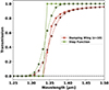 |
Fig. B.1. Transmission models of a damping wing (brown lines) and a step function (green lines) for a z = 10 source. We include the intrinsic model, re-gridded to match our R100 observations (solid lines), and the dispersed version of this model (dashed lines). The Lyα wavelength is shown by a faint vertical line. |
For λ ≫ λLyα or λ ≪ λLyα, the two convolved curves are similar (i.e. either 0 or unity). But in this case of a z = 10 source, the curves differ at λ ∼ λLyα, with a discrepancy of up to ∼20%. This strong difference can be detected for some sources, and will be used in future works to place constraints on the proximity zones and IGM neutral fraction of z > 8 sources in JADES (e.g. Jakobsen et al., in prep.). Indeed, multiple studies have now used JWST/NIRSpec observations to constrain the Lyα damping wing (e.g. Fujimoto et al. 2023; Heintz et al. 2023; Umeda et al. 2023).
Throughout this work, we assume that the transmission function for galaxies in our sample is a simple step function (i.e. 100% transmission redwards of λLyα). In reality, damping wings will affect all of the z ≳ 8 sources, resulting in low transmission at λLyα and thus making it more difficult to detect Lyα emission. For the six z > 8 sources in our sample (none of which are detected in Lyα emission), we note that this is not accounted for in our REWLyα upper limits, so these may be slightly underestimated. But a full treatment of the damping wing effect is beyond the scope of this paper and will be fully explored in a future analysis.
Appendix C: Table of best-fit parameters
Results of fitting the R100 spectra of each galaxy.
Appendix D: MUV derivation
Due to the high quality of the NIRSpec spectra, we are able to derive M1500 Å absolute magnitudes (MUV) directly from the observed data. First, the observed data are shifted from the observed to rest frame by multiplying all flux values (i.e. fλ) by 1 + z and dividing all wavelength values by the same factor. The rest-frame fλ values are converted to a fν:
 (D.1)
(D.1)
where c is the speed of light. We collected and averaged all fν values that lie between 1400 and 1600 Å (rest-frame) and used this average value ( ) to derive an apparent AB magnitude (Oke & Gunn 1983):
 (D.2)
(D.2)
which we converted to an absolute magnitude via
![Mathematical equation: $$ \begin{aligned} M_{\rm UV}=m_{1500}-5\log _{10}(D_L[Mpc])-25. \end{aligned} $$](/articles/aa/full_html/2024/03/aa47099-23/aa47099-23-eq10.gif) (D.3)
(D.3)
An error was estimated by calculating the root mean square noise level of the fν values between 1400−1600 Å from the error spectrum and perturbing  by this value.
Appendix E: Comparison data
As one of the brightest emission lines for star-forming galaxies at high-redshift, Lyα has been studied in numerous galaxies over the past decades. While the subset of JADES that we analyse in this work offers the opportunity to explore the Lyα properties of galaxies between z ∼ 5 − 11, our conclusions are strengthened by the addition of archival data. Here, we collected a large literature sample of galaxies with reported spatial positions, spectroscopic redshifts, Lyα equivalent widths from spectral observations, and MUV values. Unless otherwise stated, zsys = zLyα and MUV = M1500. The details of our comparison sample are given below3. To avoid repeated galaxies, we searched for entries within 0.25″ of each other and excluded the older measurement.
Followup spectroscopy of bright LAEs discovered in the Systematic Identification of LAEs for Visible Exploration and Reionization Research Using Subaru HSC (SILVERRUSH) with a variety of ground-based telescopes resulted in numerous detections (Shibuya et al. 2018). The continuum level underlying Lyα was found by extrapolating from red filters (β = −2), while MUV was estimated from the observed spectra.
We also included the large survey CANDELSz7 (Pentericci et al. 2018), a large programme that observed star-forming galaxies at z ∼ 6 and z ∼ 7 in the GOODS-S, United Kingdom Infrared Telescope (UKIRT) Infrared Deep Sky Survey (UKIDSS) Ultra-Deep Survey (UDS), and Cosmic Evolution Survey (COSMOS) fields with the FOcal Reducer/low dispersion Spectrograph 2 (FORS2) on the Very Large Telescope (VLT). We included all galaxies with good quality flags (i.e. A, A/B, and B) and Lyα flux estimates. MUV values were estimated using fits to photometry from the Cosmic Assembly Near-infrared Deep Extragalactic Legacy Survey (CANDELS), while the REW was derived by fitting the observed spectra. Six sources were also observed with the VLT Multi Unit Spectroscopic Explorer (MUSE) by Kerutt et al. (2022), so they are not included.
Next, we included the results of studies that used Keck/MOSFIRE. Jung et al. (2022) observed eight z ∼ 7 − 8 galaxies in CANDELS Extended Groth Strip (EGS) and used an asymmetric Gaussian to fit the Lyα emission. We excluded one source that lacks a spectroscopic redshift and a number of galaxies with only upper limits on REWLyα. Four galaxies in this sample were likely re-observed in Tang et al. (2023), so they were also excluded. While Tilvi et al. (2020) observed three galaxies in group at z = 7.7, we took the one source with MUV calculated by Tang et al. (2023), or z8_5 (EGS-zs8-1 in Oesch et al. 2015). Song et al. (2016) detected one galaxy in Lyα emission (z7_GSD_3811), whose emission was fit with an asymmetric profile. Hoag et al. (2019) detected Lyα emission from two galaxies that are strongly lensed by galaxy clusters. Values are magnification-corrected, and equivalent width is calculated by dividing the line flux by HST WFC3/F160W continuum flux.
Keck DEep Imaging Multi-Object Spectrograph (DEIMOS) observations by Ono et al. (2012) resulted in line detections for three z ∼ 7 galaxies in the Subaru Deep Field (SDF) and GOODS-N. The continuum properties were derived from a fit to the photometry. Further Keck/DEIMOS observations revealed 36 LAEs (Fuller et al. 2020). We note that SDF-63544 is also known as IOK-1 (e.g. Iye et al. 2006). Additional Keck observations resulted in three detections of Lyα with the Low Resolution Imaging Spectrometer (LRIS) and NIRSPEC spectrograph (Schenker et al. 2012), where the continuum was estimated by extrapolating a power-law model (β = −2) from a red filter.
Two works used the VLT/FORS2 spectrograph (Cuby et al. 2003; Vanzella et al. 2011). For these, we took MUV from the compilation of Matthee et al. (2019). Additionally, the Gemini Multi-Object Spectrograph (GMOS) on the 8.2m Gemini Telescopes were used to observe one target. The resulting spectra were fit with templates, resulting in a Lyα REW and M1350.
The Binospec spectrograph on the 6.5 m MMT telescope was used to observe eight UV-bright (MUV ∼ −22) galaxies at z ∼ 7 selected from the Atacama Large Millimeter/submillimeter Array (ALMA) Reionization-Era Bright Emission Line Survey (REBELS; Endsley et al. 2022). Red bands were used to estimate the Lyα continuum, while MUV ≡ M1600.
VLT/MUSE features a bluer spectral range (0.465 − 0.930 μm4) with respect to the JWST/NIRSpec PRISM/CLEAR filter–disperser combination (0.6 − 5.3 μm), allowing it to probe Lyα to lower redshifts (z ∼ 2.8 − 6.7). Through the MUSE-WIDE and MUSE-DEEP surveys, Kerutt et al. (2022) present the Lyα equivalent widths for 1920 galaxies over the full redshift range accessible to MUSE. The continuum level at λLyα is estimated from photometry, while Lyα is measured from each MUSE data cube.
We also included ten galaxies in the Abell 2744 cluster from the recent work of Prieto-Lyon et al. (2023), who analysed data from the GLASS-JWST Early Release Science programme. MUV values were derived from spectral energy distribution fits to HST and JWST photometry, while REWLyα is taken from the MUSE observations of Richard et al. (2021). The systemic redshift is derived from fits to optical lines as observed by JWST.
Finally, we included results from the recent work of Tang et al. (2023), who used the MSA of JWST/NIRSpec (R100 and R1000) to extract spectra and continuum estimates for ten sources. Four sources feature small spatial offsets (< 0.1″) and redshift differences (δz ∼ 0.25 − 0.35) with sources observed with Keck/MOSFIRE by Tang et al. (2023). Since the redshift difference may be explained by a difference in methods (i.e. photometric versus spectroscopic), we assumed that these are the same galaxies. Here, zsys = z[OIII]5007. Lyα and continuum properties were extracted from the CEERS spectra and from photometry, respectively. The NIRSpec-based Lyα properties agree with ground-based REW measurements, suggesting the absence of calibration issues. A few of these sources were known by other names in previous studies: CEERS-1019 is EGSY8p7 (Zitrin et al. 2015), CEERS-1029 is EGS_z910_44164 (Larson et al. 2022), and CEERS-698 is EGS-zs8-2 (Roberts-Borsani et al. 2016).
Appendix F: REW-MUV simulation
In Section 4.2, we found that the REWLyα and MUV of our sample showed an apparent positive relation, such that more UV-faint galaxies featured larger Lyα equivalent widths. But since REW is a ratio of line flux to continuum flux, it is possible that this relation is influenced by the sensitivity limit of our sample and fitting method (i.e. we may miss Lyα-faint galaxies). In this section, we test this possibility using a method similar to our completeness analysis (Section 3.5).
For each survey tier (Deep/HST, Medium/HST, and Medium/JWST), we created 750 model spectra by sampling uniformly for several properties (5.6 < z < 12.0, −20.4 < MUV < −16.4, spectral slope −2 < n < 2, 0.1 < FR < 0.8) and log-uniformly for Lyα equivalent width (1 < REWLyα < 750 Å). Gaussian noise was added to each model spectrum based on the corresponding mean error spectrum, and the resulting spectrum was fit with our routine.
In Figure F.1, we show the intrinsic distribution of REW versus MUV in blue, and display the resulting best-fit values as red-outlined black circles. Upper limits on REW (3σ) are shown as downward arrows. It is clear that we do not capture the full distribution, as galaxies in the lower-right corner (UV-faint and low-REW) are not able to be fit. From this test, it is clear that our sample and fitting approach may result in a false positive trend of REW with MUV, due to sensitivity limits.
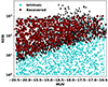 |
Fig. F.1. Results of fitting a sample of simulated galaxies. The intrinsic distribution of REW and MUV for the simulated galaxies are shown as cyan circles, with a cyan rectangle outlining the region. The best-fit values and 3σ upper limits are shown as red-outlined circles and black arrows, respectively. |
All Tables
All Figures
|
Fig. 1. Demonstration of how Lyα break and emission for a source at z = 7 are affected by the low resolving power of our observations. The top panel shows how a step function (blue line) is affected by the resolving power on a high-resolution (Δλ = 0.001 μm) spectral grid (orange curve), and how this curve would appear on the R100 spectral grid (green steps). If we add Lyα emission with a given REWLyα in the first high-resolution spectral bin redwards of the break and then account for the LSF and R100 spectral bin, we find the curves in the lower panel. |
| In the text | |
|
Fig. 2. Results of fitting a line plus continuum model to observed JADES R100 data, for sources detected in Lyα emission (denoted by “L+C FIT”). In each top panel, we show the observed spectrum (purple line) with an associated 1σ error (shaded region). The best-fit model, which includes the effects of the LSF, is shown by a yellow line. Fitting was performed using the wavelength range that is shaded grey. The continuum value at the redshifted Lyα wavelength is represented by a brown star. The bottom panel shows the residual. Continued in Fig. A.1. |
| In the text | |
|
Fig. 3. MUV (from NIRSpec spectra; see Appendix D) versus systemic redshift (based on optical lines) for our sample. Galaxies observed in different tiers are coloured differently. Sources detected in Lyα emission are shown as diamonds with black outlines. Horizontal dashed lines show MUV values of −18.75 and −20.25, while the vertical grey line shows our lower redshift cutoff (zsys > 5.6). |
| In the text | |
|
Fig. 4. Distribution of Lyα REWs as a function of MUV for our sample (orange circles for detections and green triangles for 3σ upper limits) and from the literature (purple circles for detections and red triangles for 3σ upper limits). An illustrative fit to the detections is shown by the black dashed line. See Appendix E for details of the literature sample. |
| In the text | |
|
Fig. 5. Fraction of observed galaxies detected in Lyα emission with REWLyα > 25 Å (left), REWLyα > 50 Å (centre), and REWLyα > 75 Å (right). Derived fractions from the literature are shown by coloured markers. For the central panel, note that Stark et al. (2011) and Ono et al. (2012) used a REW limit of > 55 Å. The fractions derived using only the observed JADES galaxies are shown by black points. Our REW > 25 Å values (grey) are likely affected by low completeness. |
| In the text | |
|
Fig. 6. Cumulative distribution for Lyα REW for UV-faint galaxies (−20.25 < MUV < −18.75) at z ∼ 7. Each solid line shows the expected distribution for a model with NHI = 1020 cm−2 and a wind speed of 200 km s−1, but with a different neutral fraction (Pentericci et al. 2014). Estimates from the literature (Ono et al. 2012; Schenker et al. 2012, 2014; Pentericci et al. 2014, 2018) are shifted by 1 Å for visibility. Our P(REW > 25 Å) point (grey) is likely affected by low completeness. |
| In the text | |
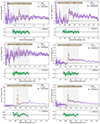 |
Fig. A.1. See the caption of Figure 2. |
| In the text | |
|
Fig. A.1. continued. |
| In the text | |
|
Fig. B.1. Transmission models of a damping wing (brown lines) and a step function (green lines) for a z = 10 source. We include the intrinsic model, re-gridded to match our R100 observations (solid lines), and the dispersed version of this model (dashed lines). The Lyα wavelength is shown by a faint vertical line. |
| In the text | |
|
Fig. F.1. Results of fitting a sample of simulated galaxies. The intrinsic distribution of REW and MUV for the simulated galaxies are shown as cyan circles, with a cyan rectangle outlining the region. The best-fit values and 3σ upper limits are shown as red-outlined circles and black arrows, respectively. |
| In the text | |
Current usage metrics show cumulative count of Article Views (full-text article views including HTML views, PDF and ePub downloads, according to the available data) and Abstracts Views on Vision4Press platform.
Data correspond to usage on the plateform after 2015. The current usage metrics is available 48-96 hours after online publication and is updated daily on week days.
Initial download of the metrics may take a while.