| Issue |
A&A
Volume 683, March 2024
|
|
|---|---|---|
| Article Number | A9 | |
| Number of page(s) | 13 | |
| Section | Extragalactic astronomy | |
| DOI | https://doi.org/10.1051/0004-6361/202346591 | |
| Published online | 28 February 2024 | |
A combined LOFAR and XMM-Newton analysis of the disturbed cluster PSZ2G113.91-37.01
1
INAF – Osservatorio di Astrofisica e Scienza dello Spazio, Via Piero Gobetti 93/3, 40129 Bologna, Italy
e-mail: This email address is being protected from spambots. You need JavaScript enabled to view it.
2
Dipartimento di Fisica e Astronomia, Università di Bologna, Via Gobetti 92/3, 40121 Bologna, Italy
3
INAF – Istituto di Radio Astronomia, Via Gobetti 101, 40129 Bologna, Italy
4
Center for Astrophysics | Harvard & Smithsonian, 60 Garden Street, Cambridge, MA 02138, USA
5
INFN – Sezione di Bologna, Viale Berti Pichat 6/2, 40127 Bologna, Italy
6
INAF – Istituto di Astrofisica Spaziale e Fisica Cosmica di Milano, Via A. Corti 12, 20133 Milano, Italy
7
INAF – Padova Astronomical Observatory, Vicolo dell’Osservatorio 5, 35122 Padova, Italy
8
Leiden Observatory, Leiden University, PO Box 9513 2300 RA Leiden, The Netherlands
9
Thüringer Landessternwarte, Sternwarte 5, 07778 Tautenburg, Germany
Received:
4
April
2023
Accepted:
27
September
2023
Abstract
In this work, we investigate the interplay between the X-ray and radio emission of the cluster PSZ2G113.91-37.01 (z = 0.371) using the high-quality XMM-Newton observations of the Cluster HEritage project with XMM-Newton – Mass Assembly and Thermodynamics at the Endpoint of structure formation (CHEX-MATE), and the images from the second data release of the LOFAR Two-meter Sky Survey (LoTSS-DR2). The cluster is undergoing a merger along the north-south axis and shows a central radio halo and two radio relics, one in the southern region and one in the northern one. Analysis of the intracluster medium (ICM) distribution revealed the presence of a northern surface brightness (SB) jump associated with the merger event. By extracting spectra across this discontinuity, we classified the edge as a cold front. Furthermore, we made use of upgraded Giant Metrewave Radio Telescope observations that allowed us to perform a spectral analysis of the G113 radio emission. We found evidence for the re-acceleration of particles in the northern relic, and we measured an associated Mach number of ℳ = 1.95 ± 0.01, as inferred from radio observations. We then performed a point-to-point analysis of the X-ray and radio emission, both in the halo and in the northern relic regions. We found a strong correlation for the halo and an anti-correlation for the relic. The former behaviour is in agreement with previous studies. The relic anti-correlation is likely related to the reverse radial distribution of the X-ray (increasing towards the cluster centre) and radio (decreasing towards the cluster centre) emissions. Finally, we performed a point-to-point analysis of the radio emission and the residuals obtained by subtracting a double β model from the X-ray emission. We found a strong correlation between the two quantities. This behaviour suggests the presence of a connection between the process responsible for the radio emission and the one that leaves fluctuations in the X-ray observations.
Key words: X-rays: galaxies: clusters / X-rays: galaxies / galaxies: clusters: intracluster medium
© The Authors 2024
 Open Access article, published by EDP Sciences, under the terms of the Creative Commons Attribution License (https://creativecommons.org/licenses/by/4.0), which permits unrestricted use, distribution, and reproduction in any medium, provided the original work is properly cited.
This article is published in open access under the Subscribe to Open model. This email address is being protected from spambots. You need JavaScript enabled to view it. to support open access publication.
1. Introduction
According to the hierarchical scenario of structure formation, clusters of galaxies form through the accretion of mass and the infall of smaller sub-structures (e.g. Frenk et al. 1983; Kravtsov & Borgani 2012). Due to the large amount of energy dissipated (up to 1063–1064 erg during one cluster crossing time, that is ∼Gyr), these phenomena have a strong impact both on the thermal and non-thermal components of clusters. The infall of matter in the cluster potential generates shock waves and cold fronts in the intracluster medium (ICM) that appear in the form of sharp surface brightness (SB) discontinuities in the X-ray observations (e.g. Markevitch & Vikhlinin 2007, for a review). These features, together with the merger-induced turbulence, are often involved in the formation of extended, cluster-scale, non-thermal structures, which are classified as radio halos or as radio relics, depending on their shape, location, and radio properties (e.g. Feretti et al. 2012; van Weeren et al. 2019, for observational reviews). In particular, radio halos are usually co-located with the main X-ray emission of the hosting cluster, while radio relics are mainly located in cluster peripheries. Furthermore, these latter are characterised by an arc-like morphology and are observed to be polarised (∼20–30% at 1.4 GHz).
The origin of these radio sources is not yet fully understood. At the moment, theoretical models (see Brüggen et al. 2012; Brunetti & Jones 2014) suggest that radio halos originate by re-acceleration mechanisms driven by merger-induced turbulence, whereas radio relics are generated by weak shocks (Mach number ℳ = 2–4). Many observations seem to agree with the predictions of these models. For example, both relics and radio halos are mostly detected in merging galaxy clusters (e.g. Buote 2001; Bruno et al. 2021; Cassano et al. 2023), and the former ones, with their arc-shape morphology and high polarisation, are often observed at the location of shocks (e.g. Akamatsu & Kawahara 2013; Botteon et al. 2016a; Eckert et al. 2016). However, the details of this global picture are still not clear. For both relics and halos, the main issues are related to the origin of the seed particle population, the (re)acceleration mechanism, and the role of the magnetic field. The weakness of the relic scenario resides in the fact that, if we assume that particles are accelerated directly from the thermal pool, the shocks detected are not strong enough to reproduce the observed relic radio spectrum and luminosity (Botteon et al. 2016b, 2020a; Eckert et al. 2017; Hoang et al. 2017). To overcome this limit, models assuming the re-acceleration of clouds of pre-existing relativistic particles in the ICM have been proposed (e.g. Markevitch et al. 2005; Kang et al. 2012; Pinzke et al. 2013). These are supported by the connection between relics and old active galactic nuclei (AGN) plasma observed in some systems (e.g. Bonafede et al. 2014; van Weeren et al. 2017). For radio halos, the open questions relate to the understanding of the complex mechanisms that drain a fraction of the energy of the large-scale turbulence generated by cluster formation events (such as mergers) into electromagnetic fluctuations and collisionless mechanisms of particle acceleration at much smaller scales (e.g. Brunetti & Lazarian 2011, 2016; Miniati & Beresnyak 2015; Sironi 2022). The definition of the role played by cosmic ray protons (CRp) and accelerated protons in the generation of these extended radio sources is also still debated (e.g. Brunetti et al. 2017; Nishiwaki & Asano 2022).
From this introduction, it appears that combined X-ray and radio analyses of a large number of galaxy clusters are needed to deepen our knowledge of the interplay between the thermal and non-thermal components of these systems. For example, the identification of a spatial correlation between the X-ray and radio SB (IX − IR) allows one to verify, and eventually to constrain, the connection between these two components (as already discussed in e.g. Govoni et al. 2001; Brunetti 2004; Pfrommer 2008; Donnert et al. 2010; Brunetti & Jones 2014). In this paper, we perform a combined X-ray and radio analysis of the cluster PSZ2G113.91-37.01 (hereafter, G113). This cluster was first detected by the ROSAT All Sky Survey (RASS, Voges et al. 1999) and is included in the meta-catalogue of X-ray detected clusters of galaxies (MCXC, Piffaretti et al. 2011) with the name of MCXC J0019.6+2517 and an associated redshift of z = 0.1353. The more recent Planck survey reassessed the cluster redshift as z = 0.3712 and measured a mass of M500 = (7.58 ± 0.55)×1014 M⊙ (Planck Collaboration XXVII 2016). Despite the ROSAT detection, no observation by any major X-ray satellite has been performed before the ones used in this work and realised by the X-ray Multi-Mirror Newton (XMM-Newton) telescope as part of the “Cluster HEritage project with XMM-Newton: Mass Assembly and Thermodynamics at the Endpoint of structure formation” (CHEX-MATE), an XMM-Newton Multi-Year Heritage program (see The CHEX-MATE Collaboration 2021, for more details1). On the radio side, new instruments able to perform deep and high-resolution imaging have only been developed in the last few years. The principal dataset used in this analysis belongs to the second data release of the fairly recent Low Frequency Array (LOFAR) Two-meter Sky Survey (LoTSS, LoTSS-DR2, Shimwell et al. 2022), an ongoing radio survey that aims to observe the entire northern sky in the frequency range 120–168 MHz with the LOFAR High Band Antennas (HBA). We refer the reader to Shimwell et al. (2017, 2019) for more details on LoTSS and its scientific goals. G113 belongs to the LoTSS-DR2/PSZ2 sample presented in Botteon et al. (2022) and shows a central radio halo, and a couple of radio relics that are developing in opposite directions. The power of combining the CHEX-MATE and LoTSS data has already been tested in a couple of cases, such as A2249 (or PSZ2 G057.61+34.93, Locatelli et al. 2020) and A1430 (or PSZ2 G143.26+65.24, Hoeft et al. 2021). This work again shows the power of the synergy between the two datasets, setting the stage for a full exploitation performed with the entire CHEX-MATE sample. Finally, we complemented our analysis with upgraded Giant Metrewave Radio Telescope (uGMRT) observations that allowed us to investigate the spectral radio properties of G113.
This paper is structured as follows: in Sect. 2, we summarise the radio and X-ray data reduction and the respective imaging processes; in Sect. 3, we describe the analysis performed to investigate the properties and correlations of the X-ray and radio emissions; and we discuss the results and draw our conclusions in Sect. 4. We adopted a flat Λ-cold dark matter cosmology with ΩM(0) = 0.3, ΩΛ = 0.7, and H0 = 70 km Mpc s−1. The scale factor at the redshift of the cluster is 5.129 kpc/″.
2. Data preparation
2.1. LOFAR observations
LoTSS pointings are characterised by a full width at half maximum of 3.96° at 144 MHz and are separated by ∼2.6°. For this reason, a specific target is usually covered by multiple pointings. In our case, the cluster G113 falls in two pointings of the survey, namely P004+26 and P005+22, which have to be combined. In order to correct for direction-independent and direction-dependent effects that are present in the data, pointings were processed with fully automated pipelines developed by the LOFAR Surveys Key Science Project team. The calibrated data used in this analysis are the same as in Botteon et al. (2022). For this reason, we refer the reader to that work for more details on the reprocessing steps. To perform the imaging of our dataset, we resorted to the WSClean v2.82 algorithm (Offringa et al. 2014). As a first step, we removed the contribution of discrete sources in the halo region by imaging the data sets with a uv cut corresponding to a physical scale of 500 kpc at the cluster redshift. By observing the model image obtained, we noticed the presence of an ambiguous radio source in the northeast part of the radio halo (see the red arrow in the central panel of Fig. 1). Due to the lack of an optical counterpart, we decided to include it in our analysis; we discuss its treatment in Sect. 3.3. The clean components of the other discrete sources co-spatial with the halo were then subtracted from the visibility data. Sources detected in correspondence of the radio relics were not subtracted. Starting from the visibility data, we produced images at different resolutions to better observe the nature and morphology of the diffuse radio emission in the ICM. In particular, we adopted the Briggs (1995) weighting scheme with robust = −1, −0.5, and −0.25, and we applied Gaussian uv tapers in arcsec equivalent approximately to 50, and 100 kpc at the cluster redshift. Furthermore, we adopted the multi-scale, multi-frequency deconvolution option (Offringa & Smirnov 2017) and subdivided the bandwidth into six channels for all imaging runs. By comparing the radio flux of the different images, we observed that the one that maximises it in the region of the radio halo is the image obtained with robust = −0.25 and taper = 100 kpc. Therefore, we decided to use this image for our analysis. The resolution and rms of the final image are 33″ × 27″and 0.37 mJy beam−1, respectively.
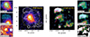 |
Fig. 1. X-ray and radio emissions of the cluster G113. In particular, central image left: a G113 XMM-Newton observation in the 0.7–1.2 keV band with LOFAR radio contours ([−3, 3, 6, 9, 12] × σ, with σ = 0.37 mJy beam−1) superimposed. The region encircled in gold shows the extension of R500. Central image right: a LOFAR image of G113 with the same contours used for the X-ray image. The resolution of the radio map is 33″ × 27″. The red arrow in the LOFAR panel shows the location of the ambiguous blob radio emission that was not subtracted from the halo emission. Subplots on the left (right) from top to bottom: a close-up of the X-ray (radio) halo region, a close-up of the X-ray (radio) northern relic region, and residuals obtained by dividing the X-ray (radio) image for the best-fit double β-model (exponential model; see Sect. 3.3 for more details). |
2.2. uGMRT observations
To investigate the spectral nature of the G113 radio emission, we analysed observations obtained with the uGMRT under project code 40_025. These were realised in Band 4 (550–750 MHz), with an observing time of ∼6 h. Data were recorded in 2048 frequency channels, with an integration time of 5.3 s in total intensity mode. The 200 MHz bandwidth was split into four frequency slices with a bandwidth of 50 MHz, centred on 575, 625, 675, and 725 MHz, respectively. Data were then processed independently using the Source Peeling and Atmospheric Modeling pipeline (SPAM, Intema et al. 2009) and setting the absolute flux density scale according to Scaife & Heald (2012). After calibration, the four slices were jointly deconvolved with WSClean. The same uv-cut used for the LOFAR observations was adopted in order to subtract discrete sources with a physical scale lower than 500 kpc (at the cluster redshift) in the halo region. The imaging of these output calibrated data are described in Sect. 3.2.
For both the LOFAR and uGMRT images, the uncertainties on the flux estimates were computed following the equation
 (1)
(1)
with σ being the rms noise of the map, Nbeam the number of independent beams within the considered region, ξcal the calibration error, and ξsub the error associated with the source subtraction. This latter was computed by estimating the ratio between the flux density measured before and after the subtraction in the regions where discrete point sources were detected and subtracted. It was included only in the estimation of the halo emission errors, and not in the relics one. No subtraction was applied to these latter diffuse radio sources. We adopted ξcal = 10% and ξsub = 4% for LOFAR images, and ξcal = 5% and ξsub = 3% for uGMRT ones.
2.3. XMM-Newton observations
The observation data file (ObsID: 0827021001) was downloaded from the XMM-Newton archive and processed with the XMMSAS (Gabriel et al. 2004) v18.0.0 software for data reduction. The production of calibrated event files from raw data was realised by running the tasks emchain and epchain. We only considered single, double, triple, and quadruple events for MOS (i.e. PATTERN ≤ 12) and single events for pn (i.e. PATTERN ≤ 4), and we applied the standard procedures for bright pixels and hot column removal (i.e. FLAG==0) as well as pn out-of-time correction. The background subtraction was performed by removing, step by step, all the individual background components. First, we removed the photon X-ray background (i.e. unresolved cosmological sources plus the Local Bubble and the Galactic halo). The contribution of this component was estimated by simultaneously fitting the XMM-Newton data within R500 with the ROSAT All-Sky Survey spectrum extracted from the region just beyond the virial radius, using the tool available3 on the HEASARC webpage. Then, we produced an image of this component, based on the predicted count rate per pixel and accounting for the XMM-Newton vignetting as derived from the calibration files, and we subtracted it from the raw image. Second, we removed the contribution of the quiescent particle background by subtracting the image obtained from the re-normalised filter-wheel-closed observations, following the procedure explained in Zhang et al. (2009). Finally, we removed the contribution of the residual soft protons by producing an image of these components based on the expected count rate per pixel, which was determined by adding a power law component (with both the slope and normalisation free to vary), folded only with the redistribution matrix file, to the background modelling of the spectra within R500. The net exposure time obtained after cleaning is: 54.2 ks, 53.5, and 49.4 ks for the mos1, the mos2, and the pn, respectively. To detect the point-like sources we first used the edetect-chain task, then we visually checked the result. We noticed that a bright source located in the southern part of the core was not identified by the task. We decided to include it in our analysis; we investigate and discuss its nature in Sect. 3.1.
The final images used in this work are filtered in the [0.7, 1.2] keV energy band and are characterised by a binning of 50 physical pixels, which corresponds to a pixel size of 2.5″. The holes related to point-like source subtraction were filled using the dmfilth CIAO task.
3. X-ray and radio analyses
3.1. Analysis of the ICM distribution
According to the morphological classification performed in Campitiello et al. (2022), G113 is one of the most disturbed systems of the CHEX-MATE sample, with concentration  , centroid shift
  , and M = 0.74. This latter quantity (M) is a combination of c, w, and of the power ratios of order P2/P0 and P3/P0. We refer the reader to Campitiello et al. (2022) for more details on the definition of all these parameters. The XMM-Newton image of the cluster confirms that this system is undergoing a merger along the N-S axis, and from a first visual check an edge in the X-ray SB distribution, located in the northern direction, stands out. We thus extracted a profile across this region using the northern sector, N, shown in Fig. 2 (left panel). The software used in this step of the analysis was the python package PYPROFFIT (see Eckert et al. 2020, for more details). The SB profile of this discontinuity was then modelled, assuming that the underlying density profile follows a broken power law (e.g. Markevitch & Vikhlinin 2007 and references therein) and that, due to the energy band of our observations, the temperature and the abundance are uniform. In the case of spherical symmetry, the downstream and upstream (subscripts d and u) densities differ by a compression factor, 𝒞 = nd/nu, at the distance of the jump rj:
 (2)
(2)
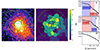 |
Fig. 2. Surface brightness edges in G113. Left: X-ray image of G113. The green regions represent the three sectors adopted for the extraction of the SB profiles. The solid black lines represent the position of the edge and the boundary of the inner sector where the temperature was measured. The dashed black lines instead represent the boundary of the outer sector where the temperature was measured. Centre: 2D temperature map of G113. The colorbar is in keV units, and the red arrow shows the position of the cold region detected in the cluster. Right (from top to bottom): SB profiles extracted in the northern (N), eastern (E), and western (W) sectors. The continuous black lines represent the best fit of the eastern (χ2/d.o.f. = 0.801 and C = 1.94 ± 0.17), northern (χ2/d.o.f. = 1.56 and C = 1.9 ± 0.2), and western (χ2/d.o.f. = 7.02 and C = 1.14 ± 0.04) jumps. The temperatures reported in the blue and red boxes are in keV units and are the temperatures measured before and after the SB discontinuities. The corresponding blue and red shaded areas show the regions where the temperatures were measured. |
where α1 and α2 are the power law indices, n0 is a normalisation factor, and r denotes the radius from the centre of the sector. The centre of the sector was chosen in order to optimise the detection of the edge. All these quantities were free to vary during the fitting procedure. Our result confirms the presence of a jump in the northern region of the cluster, with 𝒞 = 1.9 ± 0.2 (χ2/d.o.f. = 1.56). The position and angular extension of this discontinuity is shown in Fig. 2 (left panel, solid black line in the N sector). In order to investigate the nature of the jump we first made a 2D temperature map of the cluster using the Voronoi tessellation method. To define the Voronoi map bins, we considered the WVT algorithm provided by Diehl & Statler (2006), which is a generalisation of the Voronoi binning algorithm in Cappellari & Copin (2003). We required a signal to noise ratio (S/N) of S/N ∼ 30, which allowed us to estimate the temperature with a statistical uncertainty of 10–20% (see Lovisari & Reiprich 2019 for more details). We then measured the projected temperature in each region of the map. The final result is shown in Fig. 2 (central panel), while the associated error map is shown in Fig. A.1 (right panel). We found that a cold region T ∼ 5 keV is visible in the northern part of the cluster. However, due to the coarse Voronoi tessellation, it was not possible to clearly understand whether or not it corresponds to our SB discontinuity. Thus, we extracted a spectra from two annuli with S/N ∼ 50, selected with the same aperture and centre used for the extraction of the SB profile, and covering the region before and after the discontinuity. We then fitted the spectra with an APEC thermal plasma model with an absorption fixed at nH = (2.96 ± 0.08)×1020 cm−2 (Bourdin et al., in prep.), and then measured the projected temperature in each region of the map. We found a temperature of T = 6.6 ± 0.3 keV in the inner sector and a temperature of T = 9.7 ± 0.6 keV in the outer one. In order to understand whether this feature is due to the presence of a cool core and is thus a general property of the whole profile, we also extracted SB profiles from the eastern (E) and western (W) regions. We excluded the southern region due to its extended tail of X-ray emission. We found that another jump, of magnitude 𝒞 = 1.94 ± 0.17 (χ2/d.o.f. = 0.801), is present in the E direction. To investigate its nature, we extracted a temperature profile using the same procedure described for the N sector. We found an inner temperature of T = 14 ± 2 keV and an outer temperature of T = 9 ± 1 keV. In the western region, no SB discontinuity was detected. In particular, by fitting the SB profile we found a jump of magnitude 𝒞 = 1.14 ± 0.04 and a χ2/d.o.f. = 7.04. This latter parameter shows that this model is not able to properly fit the profile. Also in this case we measured the temperature using the same radial range adopted for the eastern discontinuity. We found an inner temperature of T = 6.1 ± 0.4 keV and an outer temperature of T = 8 ± 1 keV. The results arising from the analysis of these three sectors prove that the edge detected in the northern region is not tracing an overall property of the core. We thus classified the northern edge as a cold front. With regard to the eastern discontinuity, we noticed that the temperatures measured in the eastern sectors are higher than the ones measured in the western ones. Furthermore, the eastern sector used for the extraction of the SB and temperature profiles covers the region where the ambiguous radio source presented in Sect. 2.1 (row arrow in Fig. 1) is located. The temperature gradient observed, with a high temperature in the inner annulus and a lower temperature in the outer one, may be due to either the presence of an AGN or the accretion of a small sub-clump of galaxies that generates a shock. We estimated the Mach number that, if confirmed, this shock would have. Using the Rankine–Hugoniot conditions (see, e.g. Markevitch & Vikhlinin 2007), we can link the density and temperature jump to the Mach number through the relations
 (3)
(3)
and
![Mathematical equation: $$ \begin{aligned} \mathcal{M} ^2 = \frac{(8T_{j}-7)+[(8T_{j}-7)^2+15]^{1/2})}{5} \end{aligned} $$](/articles/aa/full_html/2024/03/aa46591-23/aa46591-23-eq6.gif) (4)
(4)
where Tj is the ratio between the temperature post- and pre-shock. From Eq. (3) we found ℳ = 1.68 ± 0.14, while from Eq. (4) we found ℳ = 1.55 ± 0.04. Considering the uncertainties, these two estimates are in agreement. However, the hypotheses provided are just hints for possible interpretation; further investigations are needed to understand whether the radio and X-ray emission are linked and to derive any conclusion.
The temperature map also revealed the presence of another cold region, located in the southern part of the cluster and characterised by a temperature, T, ∼4 keV. This corresponds to an X-ray clump that was not identified as a point source during the imaging of the XMM-Newton images (see Sect. 2.3). By consulting optical images from the DESI Legacy Imaging Surveys4, we noticed the presence of two foreground galaxies located at redshift z = 0.133. This may explain the original wrong RASS estimation of the cluster redshift, which was assessed to be z = 0.1353 instead of z = 0.370 (see Sect. 1).
3.2. Analysis of the diffuse radio emission
From a radio point of view, G113 represents a rare case of a cluster hosting both a central radio halo and a pair of developing radio relics, one in the northern region of the cluster and one in the southern region. The axis on which these two latter structures lie traces the direction of the merger event that is affecting the cluster and that is visible in the X-ray images (see Sect. 3.1).
In order to investigate the properties of the non-thermal emission of G113, we made a spectral index map. To achieve this goal, we produced LOFAR and uGMRT images with a common inner uv-cut to compensate for the different interferometer uv-coverage, which is critical for the recovery of the extended emission (e.g. Bruno et al. 2023). Furthermore, we adopted the same input parameters (multiscale, robust, and taper) presented in Sect. 2.1, and we fixed the shape of the restoring beam in order to have a final resolution of 35″ × 35″ in both images. We then re-gridded the two images to the same pixel grid (i.e. the LOFAR one). The rms noise of the maps is σ = 0.30 and σ = 0.037 mJy beam−1 for the LOFAR and uGMRT images, respectively, and pixels with flux values lower than 2σ were masked for each frequency. The spectral index map was then obtained by computing for each pixel the α index, defined as  , where S is the flux density and ν the considered frequency. The associated uncertainties were obtained using the relation
 (5)
(5)
The final spectral index map is shown in Fig. 3 (left panel), while the associated error map is reported in Fig. A.1 (left panel). It is possible to observe that the spectral index measured in the halo region varies between −0.8 and −2. We also noticed that higher values of α (i.e. α ≥ −1) seem to mainly be found in the southern and northwest regions of the halo. We thus extracted a profile of α across four sectors covering the northern, southern, western, and eastern regions of the radio halo. The results, together with the sectors adopted, are shown in Fig. 4, and the associated uncertainties are 1σ errors. By looking at the central value measured in each annulus of the considered sectors, it seems that a steepening of α is present. Furthermore, the spectral index measured in the northern and southern regions seems to follow a different trend; however, the uncertainties of the map do not allow us to clearly confirm this behaviour.
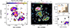 |
Fig. 3. Analysis of the radio emission of G113. Left: spectral index map of the cluster G113, with LOFAR contours of the image at 35″ × 35″ overplotted ([−3, 3, 6, 9, 12] × σ, with σ = 0.37 mJy beam−1). Centre: uGMRT image of G113, with LOFAR contours overplotted. The resolution of the image is 35″ × 35″ and the rms noise is σ = 0.037 mJy beam−1. Right top: distribution of the spectral index extracted from square-shaped boxes of width 35″ in the halo (grey) and southern relic (orange) regions. The vertical lines represent the α median values for the halo (black) and relic (orange). Right bottom: values of α extracted from the sector shown in the subplot. The sectors are numbered from the outer annulus (1) to the inner one (4). |
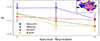 |
Fig. 4. Radial profile of α in the radio region. The four profiles refer to four different sectors that cover the northern, southern, eastern, and western regions, as shown in the cluster subplot. |
The location of the X-ray discontinuity (close to the northern boundary of the radio halo) does not allow us to obtain an accurate estimate of the variation in the α index across the cold front. In the bottom plot of Fig. 3 (right panel) we report the spectral index values extracted from square-shaped boxes with width 35″ (that is the beam width of the map) covering the halo region. We estimated a mean α value of −1.2, and an associated standard deviation of σα = 0.2. This value is more than two times higher than the median α error, αerr ∼ 0.09, measured in the whole halo region, and thus suggests that the observed variations are not (only) related to systematic errors, but are linked to the presence of intrinsic small-scale fluctuations in the spectral index across the halo. A similar behaviour was already observed in, for example, Botteon et al. (2020a), Rajpurohit et al. (2023), but not in others (e.g. van Weeren et al. 2016). In relation to the northern relic, we observed an evident steepening of the spectral index towards the cluster centre. To properly characterise this behaviour, we computed the average value of α in the four concentric rings shown in the cluster subplot of Fig. 3 (bottom right panel). Moving from north to south, the trend observed consists of first a decrease in α (from the outer annulus marked as 1 to following one) followed by a subsequent increase (from the annulus 2 to the inner annuli 3 and 4). By assuming that the particles are being accelerated via dynamic site acceleration (DSA) by a shock that is moving outwards, we can use the spectral index measured in the outer annulus (1) to estimate the Mach number, ℳ (Blandford & Eichler 1987). The relation that links α to ℳ is
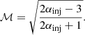 (6)
(6)
Starting from αinj = −1.21 ± 0.07, measured in the outer annulus, we found ℳ = 1.95 ± 0.01. The α steepening observed between the annuli 1 and 2 can be explained by synchrotron ageing. The subsequent increase in α may instead be related to the presence of a radio source that is injecting electrons in the surrounding regions, and that is visible in images with higher resolution (see Fig. B.1). By looking for an optical counterpart, we verified that this source corresponds to a galaxy located at the cluster redshift (z = 0.315). Finally, no peculiar trend of the spectral index is found in the southern relic. We thus computed the median α and standard deviation values using the same approach adopted for the radio halo and found α = −1.3 and σα = 0.2. In this case, too, the distribution of the spectral index measured in the squared-shape boxes is shown in the histogram of Fig. 3 (top right panel).
3.3. Point-to-point correlations
Looking for the presence of a spatial correlation between the X-ray and radio emissions is a powerful tool with which to investigate the relation between the thermal and non-thermal cluster components (Brunetti & Jones 2014). As it is possible to observe from Fig. 1, the thermal and non-thermal emission of the radio halo are basically overlapped. Many studies based on the point-to-point analysis of these two components have shown that usually the X-ray and radio flux density of the halo region follow a relation of the type  , with k < 1 (e.g. Feretti et al. 2001; Govoni et al. 2001; Giacintucci et al. 2005; Botteon et al. 2020b; Bruno et al. 2021).
In order to investigate this behaviour in G113, we performed a point-to-point analysis using the python code PT-REX described in Ignesti (2022). Based on a given threshold in SB, the code generates a sampling mesh, the cells of which reproduce the dimensions of the beam. For each cell, the values of IR and IX and their associated errors are computed. Finally, data are fitted with a power law and the Pearson (ρp) and Spearman (ρs) coefficients are estimated. We applied this procedure to the G113 halo region and found that, if all the cells of the grid with a radio signal higher than 2σ are considered, no strong correlation is observed (ρp = 0.17 and ρs = 0.22). However, by observing the plot in Fig. 5 (left panel), it is possible to notice that four points (shown in grey in the plot) deviate from the general trend. These four points correspond to the position of the blob of radio emission that was not subtracted from the halo emission during the imaging process (see Sect. 2, for more details). This clump has no optical counterpart and may be a remnant plasma in the ICM, or a substructure of the radio halo. To avoid contamination, we excluded these cells from the analysis and recomputed the slope k and the Spearman and Pearson coefficients. The final values are reported in Table 1. We found a good correlation between IR and IX. The k value measured is lower than the one found in other clusters. However, we have to consider that, by defining the grid to adopt for the X-ray–radio comparison, we selected only the regions where the radio signal is higher than 2σ. This threshold has been proved to reduce the impact that artefacts in interferometric radio images arising from the data processing have on the flux density estimates, especially for extended sources with low S/N (Botteon et al. 2020b). This radio-based threshold, together with the four cells excluded due to the presence of a blob of emission, does not allow us to properly cover the entire G113 X-ray emission; as it is possible to see from Fig. 1, part of the west and southwest emission is not considered in the analysis. This may produce a flattening of the correlation, since cells with low X-ray emission are not considered. By repeating the analysis with a radio threshold set to 1σ, we obtain larger uncertainties on the radio flux estimate, but we are able to retrieve a steeper slope, with k = 0.41 ± 0.08. This behaviour is in agreement with Bonafede et al. (2022), where it was found that the correlation  is steeper in the external regions of the cluster.
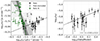 |
Fig. 5. Correlations between the X-ray and radio properties. Left: correlations between IR and IX computed in the halo (black) and northern (green) relic regions using the meshes shown in the subplots of Fig. 1. Grey points correspond to the cells excluded from the halo analysis (see Sect. 3.3). The slopes and Spearman and Pearson coefficients measured are reported in Table 1. The shadowy regions represent the scatter of the relic correlation (from dark to light grey, 1, 2, 3σ). Right: the correlation between the radio emission and the X-ray residuals. |
Results of the point-to-point analysis obtained for the halo and the northern relic.
We then tested this method on the northern and southern relics, too, in order to understand whether correlations between the X-ray and radio emissions are also present in these diffuse radio sources. A similar analysis was already performed for the radio relic detected in the cluster MACS J1149.5+2223 (Bruno et al. 2021). The results shows the absence of any correlation. However, the authors highlighted that the radio relic shows very peculiar features, such as an orientation of its major axis parallel (and not perpendicular) to the merger axis. For this reason, they concluded that further investigations were needed to understand if that radio source can really be classified as a radio relic. The meshes identified by the code for the S and N relics are shown in the respective subplots of Fig. 1, and cover the radio signal over 3σ. Since these radio sources are located in the outer regions of the cluster, we assessed the significance of the X-ray signal by measuring the S/N in each cell and by selecting only the ones over a specific threshold. By defining the source, background, and total counts as Cs, Cb, and Ct = Cs + Cb, and assuming a Gaussian error propagated in quadrature, the S/N is
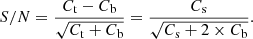 (7)
(7)
For the northern relic, we selected only the cells with S/N > 3. For the southern relic, it was not possible to satisfy this condition, since a low number of cells were included. We thus decided to exclude the treatment of this diffuse radio source from our work. By considering the selected cells of the northern relic, we found that the X-ray and radio emissions are linked by a strong anti-correlation between them. We report the k, ρp, and ρs values in Table 1, and we show the correlation and the 1, 2, 3σ scatter in Fig. 5 (left panel). We also report the position of the X-ray limits measured in the cells with S/N < 3, and we observe that few of them are not included in the 3σ scatter. By including the central values of these points in the fit, we estimated a slope of k = −1.3 ± 0.7, which is still consistent, within the uncertainties, with the one found above.
3.4. Residuals of the radio and X-ray emissions
We exploited the point-to-point analysis to investigate also the presence or absence of correlations between the residual emission obtained by dividing the X-ray and radio observations by a model emission of the thermal and non-thermal components. This analysis allows us to explore possible links between the processes that leave fluctuations in the X-ray and radio distributions.
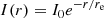
On the X-ray side, a double β-model is considered a good representation of the SB emission of those galaxy clusters that are characterised by a relaxed dynamical state. On the contrary, clusters that have been undergone merger events, AGN outbursts, or sloshing are expected to show deviations from this smooth model. By dividing the X-ray observation of G113 for the best fit model of its SB emission, we thus expect to highlight features generated by the ongoing merger event, such as substructures and discontinuities associated with shocks and cold fronts. To obtain the residuals of the X-ray emission of G113 we proceeded as follows. We resorted to the python package PYPROFFIT (see Eckert et al. 2020, for more details) to extract an averaged radial profile of the cluster. The annuli adopted for the extraction are centred on the centroid of the cluster, cover a region included in R500, and have an elliptical shape. The centroid of the cluster, the axis ratio (major/minor), and the position angle of the elliptical annuli were calculated with the principal component analysis (PCA). This method is usually used to reduce the number of dimensions needed to describe a dataset. In our specific case, it allows us to identify the two axes that hold the highest amount of variance, and that better represent the SB distribution of the cluster (that are the axes of the elliptical annuli). The ellipse axis-ratio and position angle (from the right ascension axis) found are 1.26 and 129°, respectively. We fitted the radial profile with a double β-model, using the definition
![Mathematical equation: $$ \begin{aligned} I(r)=I_0 \bigg [\bigg ( 1+ \bigg (\frac{x}{r_{c,1}}\bigg )^2 \bigg ) ^{-3\beta + 0.5} + R \bigg ( 1+ \bigg (\frac{x}{r_{c,2}}\bigg )^2 \bigg ) ^{-3\beta + 0.5} \bigg ]+B \text{,} \end{aligned} $$](/articles/aa/full_html/2024/03/aa46591-23/aa46591-23-eq15.gif) (8)
(8)
and found  ,
,  ,
,  , and
, and  . The high χ2/d.o.f. = 42.5/14 and the unusually high β confirm the extremely disturbed X-ray morphology of this system. Starting from this model, we created a vignetting-corrected model image representing the expected emission of the cluster. Finally, we divided the original X-ray image of the model in order to obtain a residual map that highlights the regions where an excess or deficiency in SB is present with respect to the model. Since both the deviations from a double β-model and the radio emission of the halo originate in the ongoing merger event, we investigated whether correlations are present between the X-ray residuals and the radio flux. To perform a point-to-point correlation between these two quantities, we considered the same grid produced by the PT-REX algorithm (see subplots of Fig. 1, which was already adopted in Sect. 3.3). In this case we also excluded the cells corresponding to the ambiguous radio blob in the halo region. For each cell included in the grid, we measured the radio flux and the X-ray residual emissions. We found a good correlation between these two quantities (see Fig. 5, right plot), with k = 0.50 ± 0.12, ρp = 0.62, and ρs = 0.51. This result depends on the model used for the description of the X-ray emission. However, a double β model centred on the centroid (which represents the centre of the potential well) of the system is expected to be one of the best possible representations to describe the SB distribution of the cluster emission. Furthermore, the plot seems to show two regimes: log(data/model) < 0.2, where IR varies in a fixed range, and log(data/model) > 0.2, where IR varies in another, higher range. We investigated whether the five points with log(data/model) > 0.2 are either spread out or related to a specific region. We found that four of the points correspond to four of the cells that cover the X-ray core. In Fig. C.1, we show in red the position of these cells.
Historically, radio halos were classified as “smooth” sources with “regular” morphologies (see Feretti et al. 2012; van Weeren et al. 2019 for the definition of a radio halo). Starting from this classification, it is common in the literature to fit the radio emission of these sources with an exponential profile defined as (Murgia et al. 2009)
 (9)
(9)
where I0 and re are the central SB and the e-folding radius, respectively. However, the new generation of radio telescopes provided us with the opportunity to study these extended radio sources with an unprecedented resolution. Recent studies highlight that, by increasing the S/N of the observations, it is possible to highlight an increasing number of deviations from this model (Botteon et al. 2022). Starting from our radio observations, we decided to investigate whether similar deviations are also visible in G113. The presented fitting of Eq. (9) and halo radio flux density estimations were done with a newly developed algorithm5, described in detail by Boxelaar et al. (2021). According to this procedure, the profiles are fitted to a two-dimensional image. This code allows both circular and non-circular models to be fitted. In comparing the results arising from a circular model and an elliptical one, we did not observe any significant difference, with the elliptical model returning almost equal semi-axes values. Given the roundish morphology confirmed by the elliptical model, and the relatively faint emission of the halo, we decided to use a circular model. The best-fit estimates of the peak SB and radius are found through Bayesian inference and maximum likelihood estimation. To sample the likelihood function, the Monte Carlo Markov chain implemented within the emcee module is used (Foreman-Mackey et al. 2013). This method allows us to find the full posterior distribution for the model parameters. An estimation of these parameters was already presented for G113 in Botteon et al. (2022). However, due to the application of a different uv-cut (250 kpc in Botteon et al. 2022, and 500 kpc in this work), the point-sources subtraction may be slightly different between the two analyses and can result in a different flux estimate. For this reason, we decided to re-perform the fit. By applying this algorithm to our cluster, we find a lower  with respect to the one found in Botteon et al. (2022;
  ). This confirms that our uv-cut leads to the subtraction of more components. As for the e-folding radius, a good agreement is found, with re = 350 ± 20 kpc in our work and re = 370 ± 15 kpc in Botteon et al. (2022). Starting from these fit results we derived a model image of the radio emission. We then obtained the radio residual image by dividing the original LOFAR image for the best-fit exponential model. Both the radio and X-ray residuals are shown in the respective subplots of Fig. 1.
As in X-rays, deviations from smooth SB models may highlight the presence of substructures or discontinuities in the radio emission. Recently, Botteon et al. (2023) has claimed that numerous radio SB discontinuities, similar to those detected in X-rays, are present in a number of radio halos observed with MeerKAT. Some of these radio edges have been found to be associated with shocks and cold fronts, suggesting a tight connection between the thermal and non-thermal components in the ICM. As merger events disturb the cluster atmosphere and dissipate energy into the acceleration of relativistic particles, we tested whether the X-ray and radio residual emissions are linked by performing a point-to-point analysis on the residual images. In this case, the meshes adopted are the same as those used in the previous analysis of the halo region. We did not find any correlation between the radio and X-ray residual emissions. This behaviour could be down to different reasons. As already shown in the literature, many radio discontinuities do not show an X-ray counterpart (e.g. Botteon et al. 2023). In these cases, the deviations from the exponential model may highlight specific regions in the ICM that are characterised by a high fraction of seed relativistic electrons or by a local enhancement of the acceleration efficiency or of the magnetic field strength. For these features, the absence of a correlation between the X-ray and radio residuals may be an indication of the fact that these two types of emission highlight different types of discontinuities. On the other hand, it has been suggested that the S/N of the observations may have a strong impact on the detection of radio edges. For example, all the radio discontinuities detected in Botteon et al. (2023) were found in clusters for which the observations have a high S/N. Given the low S/N of our observations, the lack of correlation between the X-ray and radio residuals may be related to the impossibility of detecting all the features, especially the ones that may be present in the correspondence of the X-ray substructures. Finally, we do not find any correlation between the X-ray residuals and the α index of the spectral index map.
4. Conclusions
In this paper, we performed a joint X-ray and radio analysis of the cluster G113, a merging system showing a peculiar radio morphology: besides a central radio halo, this cluster also hosts two relics perpendicular to the merger axis, one located in the northern region and one in the southern region. The double-relic configuration is used in the literature to provide good constraints on cluster merger scenarios. Currently, a dozen objects showing this feature are known (van Weeren et al. 2019), among which some well-studied cases are: Abell 3667 (Rottgering et al. 1997) and Abell 3376 (Bagchi et al. 2006), which are respectively the first and second double relics detected, and MACS J1752.0+4440 (van Weeren et al. 2012; Bonafede et al. 2012) and Abell 1240 (Kempner & Sarazin 2001; Bonafede et al. 2009).
X-ray analysis of the ICM of G113 allowed us to identify a SB discontinuity in the northern region of the cluster. By performing a spectra extraction from two annuli across the edge, we measured a downstream (i.e. post-front) temperature of T = 6.6 ± 0.3 keV and an upstream (i.e. pre-front) temperature of T = 9.7 ± 0.6 keV. We thus classified the discontinuity as a cold front.
In order to investigate the non-thermal properties of G113, we made a spectral index map. We find that the halo region is characterised by a mean α value of −1.15 and an associated standard deviation of σα = 0.23. This latter value is larger than the median error and suggests that the observed variations are linked to the presence of intrinsic small-scale fluctuations in the spectral index across the halo. We also observe a flattening of the profile in the northern front of the northern relic. This behaviour could be explained by assuming that particles are being accelerated by a shock that is moving outwards. We estimated using DSA relations that this event is characterised by a Mach number, ℳ = 1.95 ± 0.01, as inferred from the radio spectral index at the leading edge of the emission. No specific trend is observed in the southern relic. In this radio source we estimated a median α = −1.30. We then analysed the thermal and non-thermal spatial correlation by performing a point-to-point analysis of the X-ray and radio emission of the cluster. We find a sub-linear correlation between the IR and the IX of the halo region. This trend is consistent with current analysis on the X-ray and radio correlation in radio halos. We also investigated the relationship between the thermal and non-thermal spatial correlation in the northern radio relic. We find that an anti-correlation between IR and IX is present. A straightforward explanation of this behaviour could be related to the radial distribution of the X-ray and radio emissions. On the one hand, the brightest radio emission of the relic is its leading edge, which is the most distant region from the cluster centre. On the other hand, the X-ray emission decreases with the distance from the centre and is thus expected to be low (and to continue to decrease) in the relic regions. Finally, we compared the residuals obtained by dividing the X-ray and radio images into a double β model and an exponential model for the X-ray and radio emission, respectively. We find no correlation between these two quantities. However, by comparing the X-ray residual and the radio emission of the halo, we find a strong correlation. This correlation is even higher than the one between X-ray and radio SB, suggesting that the process responsible for radio emission and the one that leaves fluctuations in the X-ray images are connected. Further investigations are needed to understand which physical processes initiate this behaviour and to constrain the impact of the adopted X-ray emission model on this correlation.
Acknowledgments
We thank the staff of the GMRT who have made these observations possible. The GMRT is run by the National Centre for Radio Astrophysics of the Tata Institute of Fundamental Research. S.E., L.L., F.G., M.R, acknowledge financial contribution from the contracts ASI-INAF Athena 2019-27-HH.0, “Attivitá di Studio per la comunitá scientifica di Astrofisica delle Alte Energie e Fisica Astroparticellare” (Accordo Attuativo ASI-INAF n. 2017-14-H.0), INAF mainstream project 1.05.01.86.10, and from the European Union’s Horizon 2020 Programme under the AHEAD2020 project (grant agreement n. 871158). A.I. acknowledges funding from the European Research Council (ERC) under the European Union’s Horizon 2020 research and innovation programme (grant agreement No. 833824). R.J.v.W. acknowledges support from the ERC Starting Grant ClusterWeb 804208. M.B. acknowledges support from the Deutsche Forschungsgemeinschaft under Germany’s Excellence Strategy – EXC 2121 “Quantum Universe” – 390833306. G.B. acknowledges support from PRIN INAF Mainstream Galaxy cluster science with LOFAR. A.I. acknowledges funding from the European Research Council (ERC) under the European Union’s Horizon 2020 research and innovation programme (grant agreement No. 833824’).
References
- Akamatsu, H., & Kawahara, H. 2013, PASJ, 65, 16 [NASA ADS] [CrossRef] [Google Scholar]
- Bagchi, J., Durret, F., Neto, G. B. L., & Paul, S. 2006, Science, 314, 791 [NASA ADS] [CrossRef] [Google Scholar]
- Blandford, R., & Eichler, D. 1987, Phys. Rep., 154, 1 [Google Scholar]
- Bonafede, A., Giovannini, G., Feretti, L., Govoni, F., & Murgia, M. 2009, A&A, 494, 429 [NASA ADS] [CrossRef] [EDP Sciences] [Google Scholar]
- Bonafede, A., Brüggen, M., van Weeren, R., et al. 2012, MNRAS, 426, 40 [Google Scholar]
- Bonafede, A., Intema, H. T., Bruggen, M., et al. 2014, MNRAS, 444, L44 [Google Scholar]
- Bonafede, A., Brunetti, G., Rudnick, L., et al. 2022, ApJ, 933, 218 [NASA ADS] [CrossRef] [Google Scholar]
- Botteon, A., Gastaldello, F., Brunetti, G., & Dallacasa, D. 2016a, MNRAS, 460, L84 [Google Scholar]
- Botteon, A., Gastaldello, F., Brunetti, G., & Kale, R. 2016b, MNRAS, 463, 1534 [Google Scholar]
- Botteon, A., Brunetti, G., Ryu, D., & Roh, S. 2020a, A&A, 634, A64 [NASA ADS] [CrossRef] [EDP Sciences] [Google Scholar]
- Botteon, A., Brunetti, G., van Weeren, R. J., et al. 2020b, ApJ, 897, 93 [Google Scholar]
- Botteon, A., Shimwell, T. W., Cassano, R., et al. 2022, A&A, 660, A78 [NASA ADS] [CrossRef] [EDP Sciences] [Google Scholar]
- Botteon, A., Markevitch, M., van Weeren, R. J., Brunetti, G., & Shimwell, T. W. 2023, A&A, 674, A53 [NASA ADS] [CrossRef] [EDP Sciences] [Google Scholar]
- Boxelaar, J. M., van Weeren, R. J., & Botteon, A. 2021, Astron. Comput., 35, 100464 [NASA ADS] [CrossRef] [Google Scholar]
- Briggs, D. S. 1995, Am. Astron. Soc. Meeting Abstr., 187, 112.02 [NASA ADS] [Google Scholar]
- Brüggen, M., Bykov, A., Ryu, D., & Röttgering, H. 2012, Space Sci. Rev., 166, 187 [Google Scholar]
- Brunetti, G. 2004, in IAU Colloq. 195: Outskirts of Galaxy Clusters: Intense Life in the Suburbs, ed. A. Diaferio, 148 [Google Scholar]
- Brunetti, G., & Jones, T. W. 2014, Int. J. Mod. Phys. D, 23, 1430007 [Google Scholar]
- Brunetti, G., & Lazarian, A. 2011, MNRAS, 412, 817 [NASA ADS] [Google Scholar]
- Brunetti, G., & Lazarian, A. 2016, MNRAS, 458, 2584 [Google Scholar]
- Brunetti, G., Zimmer, S., & Zandanel, F. 2017, MNRAS, 472, 1506 [Google Scholar]
- Bruno, L., Rajpurohit, K., Brunetti, G., et al. 2021, A&A, 650, A44 [NASA ADS] [CrossRef] [EDP Sciences] [Google Scholar]
- Bruno, L., Brunetti, G., Botteon, A., et al. 2023, A&A, 672, A41 [NASA ADS] [CrossRef] [EDP Sciences] [Google Scholar]
- Buote, D. A. 2001, ApJ, 553, L15 [Google Scholar]
- Campitiello, M. G., Ettori, S., Lovisari, L., et al. 2022, A&A, 665, A117 [NASA ADS] [CrossRef] [EDP Sciences] [Google Scholar]
- Cappellari, M., & Copin, Y. 2003, MNRAS, 342, 345 [Google Scholar]
- Cassano, R., Cuciti, V., Brunetti, G., et al. 2023, A&A, 672, A43 [NASA ADS] [CrossRef] [EDP Sciences] [Google Scholar]
- Diehl, S., & Statler, T. S. 2006, MNRAS, 368, 497 [NASA ADS] [CrossRef] [Google Scholar]
- Donnert, J., Dolag, K., Brunetti, G., Cassano, R., & Bonafede, A. 2010, MNRAS, 401, 47 [NASA ADS] [CrossRef] [Google Scholar]
- Eckert, D., Jauzac, M., Vazza, F., et al. 2016, MNRAS, 461, 1302 [Google Scholar]
- Eckert, D., Gaspari, M., Vazza, F., et al. 2017, ApJ, 843, L29 [Google Scholar]
- Eckert, D., Finoguenov, A., Ghirardini, V., et al. 2020, Open J. Astrophys., 3, 12 [NASA ADS] [CrossRef] [Google Scholar]
- Feretti, L., Fusco-Femiano, R., Giovannini, G., & Govoni, F. 2001, A&A, 373, 106 [NASA ADS] [CrossRef] [EDP Sciences] [Google Scholar]
- Feretti, L., Giovannini, G., Govoni, F., & Murgia, M. 2012, A&A Rev., 20, 54 [Google Scholar]
- Foreman-Mackey, D., Hogg, D. W., Lang, D., & Goodman, J. 2013, PASP, 125, 306 [Google Scholar]
- Frenk, C. S., White, S. D. M., & Davis, M. 1983, ApJ, 271, 417 [NASA ADS] [CrossRef] [Google Scholar]
- Gabriel, C., Denby, M., Fyfe, D. J., et al. 2004, in Astronomical Data Analysis Software and Systems (ADASS) XIII, eds. F. Ochsenbein, M. G. Allen, & D. Egret, ASP Conf. Ser., 314, 759 [NASA ADS] [Google Scholar]
- Giacintucci, S., Venturi, T., Brunetti, G., et al. 2005, A&A, 440, 867 [NASA ADS] [CrossRef] [EDP Sciences] [Google Scholar]
- Govoni, F., Enßlin, T. A., Feretti, L., & Giovannini, G. 2001, A&A, 369, 441 [NASA ADS] [CrossRef] [EDP Sciences] [Google Scholar]
- Hoang, D. N., Shimwell, T. W., Stroe, A., et al. 2017, MNRAS, 471, 1107 [Google Scholar]
- Hoeft, M., Dumba, C., Drabent, A., et al. 2021, A&A, 654, A68 [NASA ADS] [CrossRef] [EDP Sciences] [Google Scholar]
- Ignesti, A. 2022, New Astron., 92, 101732 [NASA ADS] [CrossRef] [Google Scholar]
- Intema, H. T., van der Tol, S., Cotton, W. D., et al. 2009, A&A, 501, 1185 [NASA ADS] [CrossRef] [EDP Sciences] [Google Scholar]
- Kang, H., Ryu, D., & Jones, T. W. 2012, ApJ, 756, 97 [Google Scholar]
- Kempner, J. C., & Sarazin, C. L. 2001, ApJ, 548, 639 [Google Scholar]
- Kravtsov, A. V., & Borgani, S. 2012, ARA&A, 50, 353 [Google Scholar]
- Locatelli, N. T., Rajpurohit, K., Vazza, F., et al. 2020, MNRAS, 496, L48 [Google Scholar]
- Lovisari, L., & Reiprich, T. H. 2019, MNRAS, 483, 540 [Google Scholar]
- Markevitch, M., & Vikhlinin, A. 2007, Phys. Rep., 443, 1 [Google Scholar]
- Markevitch, M., Govoni, F., Brunetti, G., & Jerius, D. 2005, ApJ, 627, 733 [Google Scholar]
- Miniati, F., & Beresnyak, A. 2015, Nature, 523, 59 [NASA ADS] [CrossRef] [Google Scholar]
- Murgia, M., Govoni, F., Markevitch, M., et al. 2009, A&A, 499, 679 [NASA ADS] [CrossRef] [EDP Sciences] [Google Scholar]
- Nishiwaki, K., & Asano, K. 2022, ApJ, 934, 182 [NASA ADS] [CrossRef] [Google Scholar]
- Offringa, A. R., & Smirnov, O. 2017, MNRAS, 471, 301 [Google Scholar]
- Offringa, A. R., McKinley, B., Hurley-Walker, N., et al. 2014, MNRAS, 444, 606 [Google Scholar]
- Pfrommer, C. 2008, MNRAS, 385, 1242 [NASA ADS] [CrossRef] [Google Scholar]
- Piffaretti, R., Arnaud, M., Pratt, G. W., Pointecouteau, E., & Melin, J. B. 2011, A&A, 534, A109 [NASA ADS] [CrossRef] [EDP Sciences] [Google Scholar]
- Pinzke, A., Oh, S. P., & Pfrommer, C. 2013, MNRAS, 435, 1061 [Google Scholar]
- Planck Collaboration XXVII. 2016, A&A, 594, A27 [NASA ADS] [CrossRef] [EDP Sciences] [Google Scholar]
- Rajpurohit, K., Osinga, E., Brienza, M., et al. 2023, A&A, 669, A1 [NASA ADS] [CrossRef] [EDP Sciences] [Google Scholar]
- Rottgering, H. J. A., Wieringa, M. H., Hunstead, R. W., & Ekers, R. D. 1997, MNRAS, 290, 577 [Google Scholar]
- Scaife, A. M. M., & Heald, G. H. 2012, MNRAS, 423, L30 [Google Scholar]
- Shimwell, T. W., Röttgering, H. J. A., Best, P. N., et al. 2017, A&A, 598, A104 [NASA ADS] [CrossRef] [EDP Sciences] [Google Scholar]
- Shimwell, T. W., Tasse, C., Hardcastle, M. J., et al. 2019, A&A, 622, A1 [NASA ADS] [CrossRef] [EDP Sciences] [Google Scholar]
- Shimwell, T. W., Hardcastle, M. J., Tasse, C., et al. 2022, A&A, 659, A1 [NASA ADS] [CrossRef] [EDP Sciences] [Google Scholar]
- Sironi, L. 2022, Phys. Rev. Lett., 128, 145102 [CrossRef] [Google Scholar]
- The CHEX-MATE Collaboration (Arnaud, M., et al.) 2021, A&A, 650, A104 [NASA ADS] [CrossRef] [EDP Sciences] [Google Scholar]
- van Weeren, R. J., Bonafede, A., Ebeling, H., et al. 2012, MNRAS, 425, L36 [NASA ADS] [CrossRef] [Google Scholar]
- van Weeren, R. J., Brunetti, G., Brüggen, M., et al. 2016, ApJ, 818, 204 [Google Scholar]
- van Weeren, R. J., Andrade-Santos, F., Dawson, W. A., et al. 2017, Nat. Astron., 1, 0005 [Google Scholar]
- van Weeren, R. J., de Gasperin, F., Akamatsu, H., et al. 2019, Space Sci. Rev., 215, 16 [Google Scholar]
- Voges, W., Aschenbach, B., Boller, T., et al. 1999, A&A, 349, 389 [NASA ADS] [Google Scholar]
- Zhang, Y.-Y., Reiprich, T. H., Finoguenov, A., Hudson, D. S., & Sarazin, C. L. 2009, ApJ, 699, 1178 [NASA ADS] [CrossRef] [Google Scholar]
Appendix A: Error maps
We report in Fig.A.1 the spectral index error and the temperature relative error map.
 |
Fig. A.1. Left: spectral index error map. Right: temperature relative error map. |
Appendix B: High-resolution map
We report in Fig. B.1 a high-resolution LOFAR map of the cluster G113. The circle shows the position of the radio source that produces an increase of α in the southern boundary of the northern relic.
 |
Fig. B.1. High-resolution LOFAR image of the cluster G113. The beam size and the rms of the map are 15"×15" and σ = 0.20 Jy/beam, respectively. Pixels with values lower than 2σ were masked. The green circle highlights the presence of the radio source that contaminates the estimate of α in the spectral profile of the northern relic. |
Appendix C: Correlation between the X-ray residuals and the radio emission
In Fig. C.1 we show the location of the five points with log(data/model) > 0.2 that result from the plot of 5 (left panel). It is possible to observe that four of the five considered cells are located in correspondence of the X-ray core.
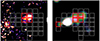 |
Fig. C.1. Left: residuals of the X-ray emission, obtained by dividing the observation for the model of the X-ray emission. The minimum of the colour scale is set to log(data/model) = 0.2. Right: LOFAR radio image of the halo region. The red cells of the grid correspond to the five points with log(data/model) > 0.2. |
All Tables
Results of the point-to-point analysis obtained for the halo and the northern relic.
All Figures
|
Fig. 1. X-ray and radio emissions of the cluster G113. In particular, central image left: a G113 XMM-Newton observation in the 0.7–1.2 keV band with LOFAR radio contours ([−3, 3, 6, 9, 12] × σ, with σ = 0.37 mJy beam−1) superimposed. The region encircled in gold shows the extension of R500. Central image right: a LOFAR image of G113 with the same contours used for the X-ray image. The resolution of the radio map is 33″ × 27″. The red arrow in the LOFAR panel shows the location of the ambiguous blob radio emission that was not subtracted from the halo emission. Subplots on the left (right) from top to bottom: a close-up of the X-ray (radio) halo region, a close-up of the X-ray (radio) northern relic region, and residuals obtained by dividing the X-ray (radio) image for the best-fit double β-model (exponential model; see Sect. 3.3 for more details). |
| In the text | |
|
Fig. 2. Surface brightness edges in G113. Left: X-ray image of G113. The green regions represent the three sectors adopted for the extraction of the SB profiles. The solid black lines represent the position of the edge and the boundary of the inner sector where the temperature was measured. The dashed black lines instead represent the boundary of the outer sector where the temperature was measured. Centre: 2D temperature map of G113. The colorbar is in keV units, and the red arrow shows the position of the cold region detected in the cluster. Right (from top to bottom): SB profiles extracted in the northern (N), eastern (E), and western (W) sectors. The continuous black lines represent the best fit of the eastern (χ2/d.o.f. = 0.801 and C = 1.94 ± 0.17), northern (χ2/d.o.f. = 1.56 and C = 1.9 ± 0.2), and western (χ2/d.o.f. = 7.02 and C = 1.14 ± 0.04) jumps. The temperatures reported in the blue and red boxes are in keV units and are the temperatures measured before and after the SB discontinuities. The corresponding blue and red shaded areas show the regions where the temperatures were measured. |
| In the text | |
|
Fig. 3. Analysis of the radio emission of G113. Left: spectral index map of the cluster G113, with LOFAR contours of the image at 35″ × 35″ overplotted ([−3, 3, 6, 9, 12] × σ, with σ = 0.37 mJy beam−1). Centre: uGMRT image of G113, with LOFAR contours overplotted. The resolution of the image is 35″ × 35″ and the rms noise is σ = 0.037 mJy beam−1. Right top: distribution of the spectral index extracted from square-shaped boxes of width 35″ in the halo (grey) and southern relic (orange) regions. The vertical lines represent the α median values for the halo (black) and relic (orange). Right bottom: values of α extracted from the sector shown in the subplot. The sectors are numbered from the outer annulus (1) to the inner one (4). |
| In the text | |
|
Fig. 4. Radial profile of α in the radio region. The four profiles refer to four different sectors that cover the northern, southern, eastern, and western regions, as shown in the cluster subplot. |
| In the text | |
|
Fig. 5. Correlations between the X-ray and radio properties. Left: correlations between IR and IX computed in the halo (black) and northern (green) relic regions using the meshes shown in the subplots of Fig. 1. Grey points correspond to the cells excluded from the halo analysis (see Sect. 3.3). The slopes and Spearman and Pearson coefficients measured are reported in Table 1. The shadowy regions represent the scatter of the relic correlation (from dark to light grey, 1, 2, 3σ). Right: the correlation between the radio emission and the X-ray residuals. |
| In the text | |
|
Fig. A.1. Left: spectral index error map. Right: temperature relative error map. |
| In the text | |
|
Fig. B.1. High-resolution LOFAR image of the cluster G113. The beam size and the rms of the map are 15"×15" and σ = 0.20 Jy/beam, respectively. Pixels with values lower than 2σ were masked. The green circle highlights the presence of the radio source that contaminates the estimate of α in the spectral profile of the northern relic. |
| In the text | |
|
Fig. C.1. Left: residuals of the X-ray emission, obtained by dividing the observation for the model of the X-ray emission. The minimum of the colour scale is set to log(data/model) = 0.2. Right: LOFAR radio image of the halo region. The red cells of the grid correspond to the five points with log(data/model) > 0.2. |
| In the text | |
Current usage metrics show cumulative count of Article Views (full-text article views including HTML views, PDF and ePub downloads, according to the available data) and Abstracts Views on Vision4Press platform.
Data correspond to usage on the plateform after 2015. The current usage metrics is available 48-96 hours after online publication and is updated daily on week days.
Initial download of the metrics may take a while.