| Issue |
A&A
Volume 682, February 2024
|
|
|---|---|---|
| Article Number | A136 | |
| Number of page(s) | 21 | |
| Section | Planets and planetary systems | |
| DOI | https://doi.org/10.1051/0004-6361/202347079 | |
| Published online | 14 February 2024 | |
The GAPS Programme at TNG
LI. Investigating the correlations between transiting system parameters and host chromospheric activity
1
INAF – Osservatorio Astronomico di Padova,
vicolo Osservatorio, 5,
35122
Padova,
Italy
e-mail: This email address is being protected from spambots. You need JavaScript enabled to view it.
2
Dipartimento di Matematica e Fisica, Università Roma Tre,
Via della Vasca Navale 84,
00146
Roma,
Italy
3
INAF-Osservatorio Astrofisico di Catania,
via S. Sofia, 78,
95123
Catania,
Italy
4
Space Research Institute, Austrian Academy of Sciences,
Schmiedlstrasse 6,
8042
Graz,
Austria
5
INAF – Osservatorio Astronomico di Palermo,
Piazza del Parlamento 1,
90134
Palermo,
Italy
6
INAF – Osservatorio Astronomico di Roma,
Via Frascati, 33,
00078
Monte Porzio (RM),
Italy
7
INAF – Osservatorio Astronomico di Trieste,
via Tiepolo 11,
34143
Trieste,
Italy
8
Instituto de Astrofísica de Canarias (IAC),
38205
La Laguna,
Tenerife,
Spain
9
INAF – Osservatorio Astrofisico di Torino,
via Osservatorio 20,
10025
Pino Torinese,
Italy
10
Instituto de Astrofísica de Andalucìa, CSIC,
Glorieta de la Astronomía,
18080
Granada,
Spain
11
Sorbonne Universités, UPMC Université Paris 6 et CNRS, UMR 7095, Institut d’Astrophysique de Paris,
98 bis bd Arago,
75014
Paris,
France
12
Dipartimento di Fisica e Astronomia Galileo Galilei, Università di Padova,
Vicolo dell’Osservatorio 2,
35122
Padova (Pd),
Italy
13
Dipartimento di Fisica, Università di Roma ‘Tor Vergata’,
Via della Ricerca Scientifica 1,
00133
Rome,
Italy
14
Max Planck Institute for Astronomy,
Königstuhl 17,
69117
Heidelberg,
Germany
15
INAF – Osservatorio Astronomico di Brera,
via E. Bianchi 46,
23807
Merate,
Italy
16
Fundaciòn Galileo Galilei – INAF,
Rambla José Ana Fernandez Pérez 7,
38712
Breña Baja,
TF,
Spain
17
INAF – Osservatorio Astronomico di Capodimonte,
Salita Moiariello 16,
80131,
Napoli,
Italy
18
INAF – Osservatorio Astronomico di Cagliari,
Via della Scienza 5,
09047,
Selargius (CA),
Italy
Received:
2
June
2023
Accepted:
14
November
2023
Abstract
Context. Stellar activity is the most relevant types of astrophysical noise that affect the discovery and characterization of extrasolar planets. On the other hand, the amplitude of stellar activity could hint at an interaction between the star and a close-in giant planet. Progress has been made in recent years in understanding how to deal with stellar activity and search for observational evidence of star-planet interactions.
Aims. The aim of this work is to characterize the chromospheric activity of stars hosting short-period exoplanets by studying the correlations between the chromospheric emission (CE) in the Ca II H&K and the planetary parameters.
Methods. We measured CE in the Ca II H&K lines using more than 1900 high-resolution spectra of a sample composed of 76 targets, observed with the HARPS-N spectrograph between 2012 and 2020. We transformed the fluxes into bolometric- and photospheric-corrected chromospheric emission ratios, R′HK. Furthermore, we completed the sample of hosts digging for data in previous works. Stellar parameters Teff, B–V, and V were retrieved homogeneously from the Gaia DR3. Then, M★, R★, and ages were determined from isochrone fitting. We retrieved planetary data from the literature and catalogs. The search for correlations between the log(R′HK) and planetary parameters have been performed through both Spearman’s rank and its statistics as well as the more sophisticated Gaussian mixture model method.
Results. We found that the distribution of log(R′HK) for the transiting planet hosts is different from the distribution of field main-sequence and sub-giant stars. The log(R′HK) of planetary hosts is correlated with planetary parameters proportional to the planetary radius to the power of n (RPn, indicating a common origin for the correlations. The statistical analysis has also highlighted four clusters of host stars with different behavior in terms of their stellar activity with respect to the planetary surface gravity. Some of the host stars have a value of log(R′HK) that is lower than the basal level of activity for main sequence stars. The planets of these systems are very close to filling their Roche lobe, suggesting that they evaporate through hydrodynamic escape under the strong irradiation of the host star, creating shrouds that absorb the core of the chromospheric resonance lines.
Key words: planets and satellites: fundamental parameters / planet-star interactions / stars: activity / planetary systems
© The Authors 2024
 Open Access article, published by EDP Sciences, under the terms of the Creative Commons Attribution License (https://creativecommons.org/licenses/by/4.0), which permits unrestricted use, distribution, and reproduction in any medium, provided the original work is properly cited.
This article is published in open access under the Subscribe to Open model. This email address is being protected from spambots. You need JavaScript enabled to view it. to support open access publication.
1 Introduction
The majority of the 5000 exoplanets known thus far have been discovered thanks to transit and radial velocity (RV) methods1 (Schneider et al. 2011). The exoplanet population displays a tremendous diversity in terms of masses, radii, and system architectures. The broad diversity among the extrasolar planets is also reflected in the range of atmospheric compositions that has been emerging from several studies on transmission and emission spectroscopy data (for a review, see, e.g., Madhusudhan 2019). The atmospheric chemical compositions of these planets are expected to provide information on different scenarios of planetary formation and evolution. A severe obstacle in gathering this information is presented by the stellar noise, mainly due to the chromospheric activity (CA) of stars. The induced stellar variability due to the interaction between the turbulent stellar plasma and the existent magnetic field causes modifications to the stellar spectral features that could be confused with planetary ones during a planetary transit or the observation of a phase curve (e.g., Ballerini et al. 2012; Robertson et al. 2015; Cegla et al. 2018; Barclay et al. 2021).
On the other hand, the stellar CA is not only a nuisance with the capability of hiding or mimicking the presence of a planetary companion and its atmospheric features; in fact, the enhancement of the CA of a stellar host is also considered to be an effect brought on by the presence of a hot-Jupiter orbiting very close to its host star via star-planet interactions (SPI) or it could be modulated or even affected by the presence of evaporating material shrouds lost by the close-in planet. The SPI can be induced by tidal and magnetic interactions (Cuntz et al. 2000). In the former case, planets can induce tidal bulges on the star with an interaction, depending on the semi-major axis of the planet, which could lead to an enhancement of the CA of the star  . In the latter case, the SPI is driven by the planetary magnetic field that interacts with the stellar magnetic field and the intensity of the interaction is
  . Also, included in this case is a possible enhancement of the host CA. The first studies on the induced activity on planet hosts were performed by Bastian et al. (2000) in the radio wavelength range and by Saar & Cuntz (2001) in the optical, with poor results due to the insufficient sensitivity of their measurements. Later, Shkolnik et al. (2003, 2005, 2008), Kashyap et al. (2008), Scharf (2010), Gurdemir et al. (2012), Pillitteri et al. (2014), and Maggio et al. (2015) reported the detection of a significant increase of stellar activity in stars hosting hot Jupiters (hot gas-giant planets orbiting very close to their host stars). However, these studies were disputed by several authors, such as Poppenhaeger et al. (2010), Poppenhaeger & Schmitt (2011), Scandariato et al. (2013), and Miller et al. (2015), who attributed those detections to biases or selection effects. Furthermore, Canto Martins et al. (2011) searched for possible effects of SPI on the stellar chromosphere and did not find any significant correlations between the chromospheric activity (CA) indicator
  and planetary parameters.
Jupiter-like planets have a hydrogen-dominated atmosphere that evaporates when subjected to the EUV radiation and X-ray (λ < 91.2 nm) produced by their stellar host. In particular, the study of hot-Jupiters gave some evidence that mass loss can be a common phenomenon (Lammer et al. 2003; Lecavelier des Étangs et al. 2004; Lecavelier des Étangs 2007; Penz et al. 2008; Sanz-Forcada et al. 2010, 2011; Locci et al. 2019). A typical example is the extreme hot-Jupiter WASP-12 (Porb = 1.09 d, Hebb et al. 2009), which is characterized by an exosphere surrounding the planet that fills its Roche lobe (Fossati et al. 2010; Haswell et al. 2012). The resulting mass loss seems to reinforce the circumstellar gas shroud that veils the host stars in some systems.
The most widely used CA indicator for F, G, and K stars is  , derived from the ratio between the Ca II H&K line-core chromospheric excess flux, evaluated by the Mount Wilson index, S, and the bolometric emission of the star (Noyes et al. 1984). Main sequence stars typically show
  , a basal level exhibited by the quiet Sun. The determination of the
  index for the Sun has been discussed by, for instance, Egeland et al. (2017), while the recent work by Milbourne et al. (2019) shows that our star had a rotational modulation amplitude
  , while the maximum variation in its chromospheric index was ~0.05 between July 2015 and October 2017, when the Sun was observed as a star by the HARPS-N solar telescope. Such amplitudes of variation appear to be broadly similar to those observed by Baliunas et al. (1995) in low-activity main sequence stars with a colour index comparable to the Sun over three decades. Therefore, they can be regarded as representative of the intrinsic variations in the
  index of quiet solar-like stars.
The anomalously low value of the WASP-12’s Ca II H&K line-core flux  is interpreted as due to the presence of a circumstellar shroud of gas that is able to depress the stellar chromospheric flux to the observed level (Fossati et al. 2013). In subsequent works, other hosts of close-in planets were presented with values of
  and they all are likely viewed through shrouds of circumstellar gas coming from planetary atmosphere ablation (Staab et al. 2017; Haswell et al. 2020).
Following the study of Knutson et al. (2010) and considering a sample of 39 transiting planets, Hartman (2010) reported a correlation between the stellar CA  and the planetary surface gravity of transiting hot Jupiters (HJs) with a confidence level of 99.5%. Specifically, this author found that the chromospheric emission index is lower for stars with planets with lower surface gravity. In the following years, Figueira et al. (2014) reviewed the
  correlation by collecting the available data on
  and stellar and planet properties and re-evaluated the correlation in the light of an extended dataset (108 transiting planets). A theoretical model was elaborated by Lanza (2014) to explain this correlation. In that model, the planetary material, ablated by the action of the UV radiation of the host star spreads towards the star along the magnetic field lines of the extended stellar corona in which the planet is lodged. The material is retained by the magnetic field lines forming prominence-like structures able to absorb at the core of chromospheric resonance lines (Mg II h&k, Ca II H&K). Strong absorption of the chromospheric resonance lines reduces the measured value of the
  indicator and the effect is stronger when the gravity of the planet is lower, explaining the correlation.
Exploiting a set of 41 transiting hosts, Fossati et al. (2015) improved the Lanza (2014) model by treating the sample of stars as a mixture of two subsets with intrinsic CA above or below the Vaughan-Preston gap (Vaughan & Preston 1980) observed for solar-like stars. Collier Cameron & Jardine (2018) highlighted an alternative explanation for the existence of the CA versus planetary surface gravity correlation, interpreting it as a direct consequence of the resulting distribution of orbital distances for transiting planets. Collier Cameron & Jardine (2018) found that the detection probabilities for transiting planets scale inversely with the increase of the planetary tidal migration rate, creating a statistical bias toward more massive planets being more likely to be observed around young and more active stars. Because the surface gravity of giant planets is mostly directly proportional to their mass, this hypothesis explains the correlation between CA and the surface gravity found by Hartman (2010) and confirmed by Figueira et al. (2014). However, the bimodality of the correlation proposed by Fossati et al. (2015) does not seem to be interpretable in the framework of this hypothesis.
In this paper, we evaluate  for an extended sample of 76 transiting planet hosts observed over a time frame of about 9yr by the Global Architecture of Planetary Systems (GAPS; Covino et al. 2013) collaboration. To this sample, we added original SHK data from other 60 transiting hosts drawn from the literature. Finally, we evaluated, in a uniform way, the
  value for both samples to review several correlations between
  and planetary parameters using this extended dataset.
The observations and data of this study are described in Sect. 2. In Sect. 3, we provide a description and characterization of the host stars. In Sect. 4, we explain how we obtained the chromospheric index for each star and the method used to evaluate the same for the data obtained by previous works. In Sect. 5, we discuss the time variation in the CA for the GAPS targets and we put the transiting hosts into the context of the other stars in Sect. 6. Finally, in Sects. 7 and 8, we present our analysis. In Sect. 9, we give our summary and conclusions.
2 Observations and data
The GAPS project is an Italian collaboration aimed at exploiting the HARPS-N spectrograph (Cosentino et al. 2012) at the Telescopio Nazionale Galileo (TNG) to search for new planets in known planetary systems and around other peculiar stars (of low metallicity and M stars) by means of high precision radial velocity time series. The project began in 2012 and completed its first phase in 2017, after 5 yr of observations. The second phase of GAPS started in 2017, triggered by the implementation of the new TNG observing mode GIARPS (Claudi et al. 2016, 2017), which allows for the simultaneous use of HARPS-N and GIANO-B, covering both the optical (380–690 nm) and near-infrared (970–2945) wavelength ranges at the same time. In this second phase, GAPS has been devoted to studies of young planets (Carleo et al. 2018, 2020; Damasso et al. 2020; Benatti 2021; Nardiello et al. 2022) and planetary atmospheres (Borsa et al. 2019; Pino et al. 2020; Guilluy et al. 2020; Carleo et al. 2022), and this project is still ongoing. In both phases of GAPS, planetary systems with transiting planets were observed, in some cases collecting quite long time series of spectral data that have also proven useful in characterizing the CA level of such targets. In this study, we consider 76 transiting planet hosts observed in the past years by GAPS, to which we added 19 objects available from Knutson et al. (2010), and Staab et al. (2017), along with another 41 objects taken from Figueira et al. (2014). The complete sample contains 136 objects.
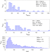 |
Fig. 1 GAPS observations of transiting hosts considered in this work. Top: number of spectra per star of the GAPS sample of transiting hosts. Middle: number of observing nights per star. Bottom: S/N value per star. |
2.1 GAPS sample
The 76 stars in the original GAPS sample were regularly monitored with the spectrograph HARPS-N since 2012, collecting data for about five to 8 yr, in some cases. In the following, we discarded four objects (KELT-7, KELT-9, KELT-20, and WASP-33) for the reasons explained in Sect. 4. The journal of the observations for the remaining 72 objects is reported in Table A.1, including the date, T0, in which the target has been observed for the first time, the total time span in days covered by GAPS data, and the number of available HARPS-N spectra. Figure 1 shows the distribution of spectra per star (top panel) and the distribution of the number of observing nights per star (central panel). For the transiting planets hosts, we have a total of 1910 spectra gathered in 867 observing nights, with a minimum of two spectra for WASP-3 and the highest number of spectra (123) for HD189733. The median is 21 spectra per star. The high number of spectra obtained for some stars is due to the frequent observing cadence during the planetary transit night we observed to detect the Rossiter-McLaughlin effect on the radial velocity curves (e.g., Esposito et al. 2017). This is the case of WASP-11 with 26 spectra taken in one night, while the maximum number of nights has been devoted to XO-2N observed for 56 nights in about 3 yr.
The main aim of the GAPS observations is to obtain precise radial velocity (RV) measurements for new exoplanet detections. To achieve this goal, in our observations, we exploited the simultaneous reference technique using both optical fibers: the target fed the first fiber, while the second fiber was illuminated by a stable calibration source, either ThAr or Fabry Perot lamp2. If the stars are fainter than 11 mag, we used the second fiber instead for sky subtraction to avoid lamp pollution. The typical exposure time was 900 s to average out solar-like pulsations. The median value of the V magnitude of GAPS targets is 11.2 mag, so the median value of the reached signal-to-noise ratio (S/N) is 44 (see the bottom panel of Fig. 1). For the brighter tail of the target distribution, the single observations can reach S/N > 100 per pixel at 550 nm, to achieve a radial velocity precision of 1 ms−1 or better, depending on the airmass of the observation and the weather conditions. The spectra were reduced through the HARPS-N data reduction software (DRS), including the radial velocity extraction based on the cross-correlation function (CCF) method (Pepe et al. 2002), where the observed spectrum is correlated with a binary mask matching the spectral type of each object. With a dedicated pipeline implemented at the INAF Trieste Observatory3 through the YABI workflow interface (Hunter et al. 2012), for the GAPS component of the sample, we also evaluated the CA index from the H&K lines of Ca II (S-index and  ), through the procedure described in Sect. 4.
2.2 Objects from previous similar works
We gathered other transiting planet hosts for which S-indices and/or  values are available in the literature (see Table 1).
We did not take into consideration the set from Canto Martins et al. (2011) because the data are not homogeneous with the previous ones. Furthermore, those objects are not transiting their stars and the measured planetary masses are just minimum masses.
In summary, we selected from Knutson et al. (2010) 18 objects (with the measured S-index value) that are not included in the list of GAPS targets and another 40 objects (with no S-index) from Figueira et al. (2014) that are not included in either GAPS or Knutson’s lists. Furthermore, we take into consideration the other two objects (WASP-72 and WASP-103) from Staab et al. (2017) for which the S-index values are given. Finally, the sample of 72 GAPS objects includes 43 stars already listed in previous works and 29 new entries. The complete target list considered in this study consists of 132 objects.
For homogeneity, we would like to evaluate the  from the original value of the S-index, using the stellar parameters that we obtained for all systems by the Gaia DR3 (see Sect. 3). Generally, the discovery papers reported in a few cases the complete time series of the SHK. This was the case of the following systems HAT-P-27, HAT-P-28, HAT-P-33, HAT-P-34, HAT-P-35, HAT-P-39, HAT-P-40, HAT-P-41, HAT-P-44, HAT-P-45, HAT-P-46, and HD97658 - for which we evaluate the mean value of SHK. Instead, for the following systems, 55 Cnc, HAT-P-25, HAT-P-38, Kepler-19, Kepler-62, Kepler-68, WASP-22, and WASP-23, the bibliography reported only a single value of SHK. For the remaining systems, when possible, we evaluated the SHK value from the available values of
  and the B–V used by the paper authors. This was the case of: Kepler-10, Kepler-17, Kepler-78, WASP-5, WASP-15, WASP-58, WASP-70 A, and WASP-84. Not all the papers outline the value of B–V used in evaluating the
  , but most of them report the Teff. We used the latter parameter to obtain the value of B–V and then the value of SHK from Modern Mean Dwarf Stellar Color and Effective Temperature Sequence by Mamajek (2021, Pecaut & Mamajek 2013)4. These systems are: Kepler-25, Kepler-48, Kepler-93, WASP-7, WASP-16, WASP-41, WASP-42, WASP-52, WASP-117, and Kepler-16. Due to the binarity of the latter system, the value of SHK obtained is pretty uncertain. Finally, for Kepler-20, we obtain the value of B–V from Zacharias et al. (2012). All the hosts are listed in Table 2 with the bibliography used.
Compilations of  measurements for planetary host stars.
3 Stellar parameters
We used Gaia/DR3 (Gaia Collaboration 2016, 2018, 2023) to obtain the values of the G magnitude and Bailer-Jones et al. (2021) for the distance of all the targets in our sample5. We found that only four stars of our sample (55 Cnc, HD 189733, HD 209458, and HD 97658) require the saturation correction described by Riello et al. (2021) for the G mag. Once applied, the correction for G is 0.002 mag for all four stars. The retrieved distances range from a minimum of 9.77 pc (GJ 436) to a maximum of 990.44 pc (Kepler-8) with a median of 221.12 pc (see the upper panel of Fig. 2). Thus, 85% of the sample is at a distance larger than 100 pc from the Sun.
We used the procedure exploited in developing the PLATO Input Catalog (PIC, Montalto et al. 2021) to retrieve the stellar parameters of the hosts homogeneously. We derived the (B – V)0 colors from the intrinsic GBP – GRP Gaia DR3 color by inverting the cubic equation reported in Table 2 of Evans et al. (2018). The reddening correction was obtained by interpolating the reddening map of Lallement et al. (2019, 2022), using the distances from Bailer-Jones et al. (2021). The effective temperatures of the stars were obtained from our custom-calibrated Gaia intrinsic color-effective temperature relationship used for the PIC.
The error in the color (median uncertainty of 3.6%) accounts for the reddening uncertainties as deduced from the reddening map, while the error on the temperature is derived from a Monte Carlo simulation, randomizing the input color within its uncertainties assuming normal error distribution and repeating the temperature calculation as described above. A normal random perturbation with a standard deviation equal to 200 K is added to the Monte Carlo temperature estimates to account for the expected difference between our temperature scale and literature results. All the details about this procedure are described in Montalto et al. (2021). In this way, we have a homogeneous determination of the Teff for most of the targets in the sample, with a trade-off of a median uncertainty of 3.5%. This is about four times the relative error for the determination of the Teff listed in the SWEET Catalog6 (Santos et al. 2013; Sousa et al. 2018, 2021), but as these authors warn, these data are not homogeneous. In the catalog, only those systems with the SWFlag= 1 can identify the stars with derived spectroscopic parameters in a homogeneous way by Sousa et al. (2021). Furthermore, we transformed the Gaia G magnitude to Johnson V magnitude using the relation by Evans et al. (2018). The middle and bottom panels of Fig. 2 show the distribution of the apparent V magnitude and of the Teff of the whole sample, respectively. The stars have apparent magnitude ranging 5.9 ≤ V ≤ 14.3 mag, with a median of 11.6 mag, while the temperature range is 3461 ≤ Teff ≤ 6781 K. We evaluated the spectral type of each member of the sample by exploiting the table from Pecaut & Mamajek (2013). The sample comprises 49 F stars, 42 G stars, 39 K stars, and 2 M stars.
For a small subset of our sample (27 stars), we considered the metallicity homogeneously derived through the methodology described in Biazzo et al. (2022) and based on iron lines. For the other hosting stars, since no homogeneous metallicities were obtained in the literature, we considered the values listed in SWEET-Cat and derived through similar spectroscopic methods identified by SWFlag= 1 (see, e.g., Sousa et al. 2021). Figure 3 shows the distribution of [Fe/H] spanning between −0.30 and 0.48 dex with a median value of 0.010 dex and a median error of 0.04 dex.
We retrieved the values of the mass, the radius, log g, and age of the stars through the PARAM web interface7, which makes use of a Bayesian method, described in da Silva et al. (2006) applied on the theoretical isochrone set PARSEC (Bressan et al. 2012). The input parameters to the PARAM tool were the apparent magnitude V, the parallax, the Teff, and [Fe/H].
In Fig. 4 (from top to bottom), the distribution of surface gravity, masses, and radii are reported. They range between 3.92 ≤ log ɡ ≤ 4.94 with a median uncertainty of 1%, 0.27 ≤ M/M⊙ ≤ 1.51, with a median relative error of 4%, and 0.26 ≤ R/R⊙ ≤ 2.12 with an uncertainty of 5%, respectively.
The age of the sample is between 0.3 ≤ age ≤ 7.3 Gyr, with 4.3 Gyr as the median age (see Fig. 5). The median relative uncertainty on age determination is 83%. Such a high uncertainty is generally given by two orders of problems tied both to the isochrones method. The age determination with the isochrones method introduces large uncertainties due to the poor knowledge of star luminosities caused by the errors in the values of the parallaxes; furthermore, a second effect is due to the long permanence of the star on the main sequence (MS). In our case, the parallax comes from the Gaia DR3 with a small uncertainty of 0.3%. Nevertheless, Teff is also an input parameter useful for evaluating the star’s age. In this case (as already described), for most of the objects of our sample, we used the values of the Teff from the PIC, with a median error of 203 K. Such a high uncertainty on Teff has an impact on the choice of the right isochrones. Taking this into account, we selected all the ages with an uncertainty ≤ 50% (see bottom panel of Fig. 5). The peak of the distribution at 4.2 Gyr disappears, leaving a quite uniform distribution of ages.
To discern between evolved and unevolved stars in our sample, we evaluated the absolute visual magnitude for each host star taking into account their parallax. The parallax errors allow us to distinguish between M-S and slightly evolved objects. In Fig. 6, we compare the objects with the HIPPARCOS average MS fitted by Wright (2004) in the (B−V) vs. MV plane. The two dashed curves indicate the portion of the plane above the M-S by 0.45 and 2.0 mag, where moderately evolved stars fall. Some objects (33) are in the sub-giant region. Objects with a height greater than 2.0 mag are considered evolved objects, but none of the stars fall in this region. It is worth noting that this is a selection effect that limits the number of evolved stars with respect to MS stellar hosts. In fact, the planet detection around a star and the determination of the planetary mass is made hard by the RV jitter induced by magnetic activity (e.g., Wright 2005) and stellar oscillations (e.g., Hatzes 1996; Beck et al. 2015). The latter ones are typically enhanced in amplitude and periods in evolved stars together with the increasing strength of surface convective motions. Both cause an increase in the RV jitter that may conceal the Keplerian signal of a planetary companion.
For all systems, the table lists Gaia DR3 id., and (B – V), and Teff obtained by Gaia Collaboration (2018) as explained in the text.
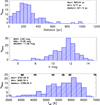 |
Fig. 2 Distributions of the stellar parameters of the GAPS sample. Upper panel: distribution of the distances of the star of the sample. Middle panel: distribution of the apparent V mag. Bottom panel: Teff distribution. The corresponding spectral types are indicated at the very top. |
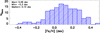 |
Fig. 3 Distribution of the spectroscopic stellar parameter: metallicities of the hosts. |
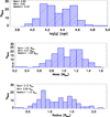 |
Fig. 4 Distribution of the stellar parameters: surface gravity (top panel), masses (middle panel), and radii (bottom panel). |
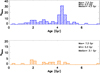 |
Fig. 5 Distribution of the stellar ages. Top panel: all hosts. Bottom panel: age distribution, considering only those with Δage/age ⊙ 50%. |
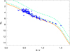 |
Fig. 6 HIPPARCOS average MS by Wright (2004) and the transiting planet hosts. Light-green dashed lines indicate loci 0.45 and 2.0 mag above the MS. |
4 Chromospheric activity of the hosts
4.1 Extracting S-index and 
To evaluate the S-index for each spectrum, we used the procedure described by Lovis et al. (2011). After the standard data reduction obtained by the DRS on-line at the telescope, this procedure performs background subtraction to correct for the diffuse light due to the ThAr or Fabry Perot lamp when we observe in simultaneous reference mode. The correction for the background is essential for the spectrophotometric accuracy and precision in evaluating the S-index. The S-index is then evaluated in the same way and with the same spectral passbands as defined for Mt Wilson Observatory spectrophotometer (Duncan et al. 1991). In particular, the Mt Wilson index is defined as:
 (1)
(1)
where H and K are the total flux in the Call H&K line cores evaluated over triangular bands centered at 393.3664 nm (K) and 396.8470 nm (H), with an FWHM of 0.109 nm. Instead, V and R are the continuum bandpasses at 390.1070 nm and 400.1070 nm, respectively, with a width of 2.0 nm. The α value is a historical conversion factor discussed in depth by Hall et al. (2007), and fixed either at 2.40 or 2.30 (Duncan et al. 1991), or adjusted following the calibration by Baliunas et al. (1995). Lovis et al. (2011) found that this S-index is equal (or very close) to the ratio of the mean fluxes per wavelength interval ( , with X representing any bandpass, and ∆λX its width in wavelength). This reduces edge effects from finite sampling at the boundaries of the bands and it leads to a value of α ~ 1 (Lovis et al. 2011). Together with the S value, its uncertainty is also computed considering the photon shot noise through error propagation. The value of the S-index obtained with HARPS (or HARPS-N) is indeed very close to the SMWO index, as can be seen by Eq. (3) in Lovis et al. (2011), with an observed difference between the two indices of 0.03.
The value of  is the chromospheric excess flux of the Call H&K lines,
  , normalized by the bolometric flux of the star (Noyes et al. 1984):
 (2)
(2)
where RHK is the stellar surface flux 𝓕HK in the Call H&K lines normalized by the bolometric stellar flux and RHK,phot is the photospheric flux contribution, 𝓕HK,phot, in the line center normalized by the stellar bolometric flux. The former is tied to the measured SMWO index via the following relation:
 (3)
(3)
where 𝓕RV is the surface flux in both the continua, while α is the same factor of Eq. (1).
The procedure on YABI measures in an automatic way the value of the S-indices of the time series obtained by GAPS for each object. In the period between 2012 Sep. 28 (JD=2456199) and 2012 Oct. 25 (JD=2456228), the HARPS-N CCD had a failure in the red chip. We did not consider the spectra taken in that period. We exploited the S-index values obtained with the procedure on YABI and derived the  values following Noyes et al. (1984). Some stars of the sample show high dispersion in the time series of
  , due to the intrinsic activity cycle or flares. These variations can be occasionally observed during intense flares, but in most of the transient events, the ranges of the
  changes are comparable or smaller than those associated with the rotational modulation or the activity cycles. Nevertheless, the sparseness of the time series in a significant fraction of our targets prevents us from identifying the individual sources of variations as seen in the
  datasets of the individual stars. To characterize the mean activity level of each of our targets, we decided to adopt the median of the observed
  timeseries of each star as the best indicator for that level. We computed also the arithmetic mean and compared it with the median to provide information on the deviation of the distribution of the
  measurements from a symmetric distribution that may suggest a preponderance of transient events. In general, these tend to increase the mean level of the
  with respect to its median. We found only three hosts (HAT-P-50, WASP-43, and WASP-50) with the average
  values differing more than 0.1 dex from the corresponding median. Moreover, the S/N of HAT-P-50 spectra is so low that we decided to exclude it from our analysis. The S-index and the corresponding
  median values are reported for each object of the GAPS sample in Table 2. We discarded KELT-7, KELT-9, KELT-20, and WASP-33 from our sample because of their high temperatures and very blue colors that are very far from the bluer limit of the calibration range of
  . Moreover, we evaluate the
  also for all the hosts for which the SHK values have been extracted by the literature (see Sect. 2.2, and Table 2).
4.2 The correction for the photospheric line flux
The  index obtained with the Lovis’ procedure underestimates the value of the activity of the star, because the photospheric flux line contribution is not fully taken into consideration in the correction by Noyes et al. (1984). This choice results in an under-correction of the photospheric flux contribution by a factor of 2 (Mittag et al. 2013), thereby leading to an underestimation of the true flux excess in the Ca II H&K lines.
To convert the S-index into absolute Call H&K chromo-spheric flux, Mittag et al. (2013) derived new color-dependent photospheric flux relation for the MS and evolved (subgiant and giant) stars in the color range between 0.44 ≤ (B − V) ≤ 1.6. This will allow us to compare different compilations of the CA indicator from the literature.
Mittag et al. (2013) derived the following relation between the continuum flux and color index B–V for the MS stars (with 0.44 ≤ B − V ≤ 1.60) and subgiant stars (with 0.44 ≤ B − V ≤ 1.10):
 (4)
(4)
With respect to the RHK,phot in Mittag et al. (2013), there are also the following relations with the color index for stars of different luminosity classes:
 (5)
(5)
This method allows for a simple and reliable conversion of the S-index and it will allow us to compare historical and new S-indices (Mittag et al. 2013).
Using the relations from Eqs. (2) to (5), we estimated the value of  for all the hosts (see Table 2). We use the suffix M to distinguish the value of
  obtained with the procedure described by Mittag et al. (2013) from that
  obtained with the procedure described by Noyes et al. (1984).
We compared the values obtained with both methods to check if they are different in a significant way. We test the difference between the two mean  values against the null hypothesis using the t-student statistic technique. It results that most of the means are significantly different with a confidence level of <0.001. The objects: HAT-P-6, HAT-P-24, HAT-P-30, WASP-3, WASP-12, WASP-31, and XO-4, have averages that cannot be considered different due to large errors that hamper the evaluation of the two
  values.
The obtained values of the CA allow us to find an empirical relation between  and
and  for the different evolutionary states of the hosts. The empirical relation will be useful to correct the classic index for the CA
  for the photospheric line flux obtaining
  when the S-indices are missing in the literature. We separated the sample into MS stars and slightly evolved (subgiant) stars as they come out from the comparison with the HIPPARCOS average MS (see Sect. 3 and Fig. 6) and for both the subsamples we search for a linear correlation between them. We take into consideration all the significant different values for all the objects in the MS with color ranging in the 0.44 ≤ B−V ≤ 1.60 interval. For the subgiant stars instead, we considered those objects with color 0.44 ≤ B−V ≤ 1.10. Figure 7 displays the comparison between the
  and
and  for the MS objects (top panel) and sub-giant stars (bottom panel) and the correlation is described by the following:
 (6)
(6)
In the following of this work, we will use the values of  , and consequently, we drop the subscript M. The distribution of the
  is shown in Fig. 8. Most of the transiting planet hosts are in the inactive and active region of the plot as they are defined by Wright (2004) and Henry et al. (1996), fewer are in the very active region, while some objects fall in the very inactive region with
  ≤ −5.1 (basal activity limit for MS stars). The upper and lower limits of our sample are respectively individuated by WASP-7
  and GJ436
  . The median value of the sample is
  held by HD 97658. This distribution follows the typical bias against very active stars of RV and (to a lesser degree) transit surveys.
5 R′HK raw dispersion and chromospheric emission variability
For the targets observed by GAPS, we have long time series of the CA indicator, but their inhomogeneity does not allow a global analysis. Nevertheless, we used the recorded variation of CA to better characterize this sample. Information on the activity variability can be obtained via the standard deviation of the stellar activity indicator. The left panel of Fig. 9 shows the distribution of the standard deviation of  (hereafter, σR5) as evaluated by the GAPS time series. The median of the distribution is 0.2 dex, and the distribution shows a tail of stars with high dispersion, possibly due to short-term variability (e.g., flares) or long-term magnetic cycles. The M2.5 dwarf GJ436 records the minimum value (0.038 dex) of the chromospheric emission (CE) variability. We observed this star on two distinct nights about 2 yr apart, so it could not be considered proof of the lowest dispersion level of our sample. Following other authors (e.g., Lovis et al. 2011; Gomes da Silva et al. 2021), we selected hosts observed on more than 20 nights on a time basis longer than 1000 days. The host with the lowest relative dispersion is HAT-P-7 (F6V) with an absolute σR5 = 0.079 dex and a relative dispersion for SMW of 2.0%. Comparing HAT-P-7 with the values for the quiet star τ Ceti: SMW/σSMW = 0.35%, obtained by Lovis et al. (2011) on a time bases of 7 yr of observations (157 nights), we can see that also HAT-P-7 could not be considered a long-term quiet star. So we have just a mere indication of the precision of our
  measurement.
Stellar activity compilations and catalogs measured for a high number of stars show that the higher envelope of activity dispersion decreases with decreasing activity level and evolutionary stage. The majority of stars have a variation in activity that ranges 0.01 ≤ σR5 ≤ 0.32 dex (Gomes da Silva et al. 2021). In our sample, there are systems with a dispersion larger than 0.5 dex (see Table 3). Among them, Qatar-2 shows the highest amplitude of variation (1.736 dex) but because of the very short time span (less than 1 day), it could be due to a flare. All the others have longer lapstime, instead.
In general, the activity variability is proportional to the level of stellar activity, and therefore, regarding age, young stars have greater activity variation than old ones. This behavior has been also highlighted by Scandariato et al. (2017) for a sample of low-activity early-type M dwarfs. The right panel of Fig. 9 reports the σR5 as a function of the  . The different colors represent the time span of the measurements. Considering only the red squares, corresponding to values with a time baseline longer than 100 days, it is possible to see that active stars have a greater spread of the CE variation. Nevertheless, some stars in the inactive zone
  exhibit a broad variation. They are WASP-1 (F9.5V), HAT-P-16 (F9V), XO-4 (F7V), HAT-P-26 (K2V), and WASP-35 (G1V). This situation seems to be corroborated by Gomes da Silva et al. (2021), who observed a high activity variation for stars of spectral types F and K with a low level of activity, as well as a larger spread of variation for the former spectral type than for the latter.
For the time being, we do not have the capacity to dig deeply into the activity variation behavior, and we leave it for future works; this is also because it is not the focal topic of this paper. In any case, the data indicate that the more active the stars, the more the activity varies. Furthermore, non-active stars could have high activity variation, in particular F stars.
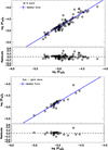 |
Fig. 7 Comparison between the values of |


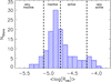 |
Fig. 8 Distribution of the |

6 Activity of planetary hosts in a general context
Figure 10 shows the distribution of the mean  obtained for each host as a function of the Teff of the stars. In this plot, it is possible to note that F stars (blue circles) have a scattered distribution with a concentration around
  . Differently, the G stars (green circles) range between
  , with a slightly high concentration around
  . Then, K stars (orange circles) show a scattered distribution in the activity range of
  . There are only two M stars (red circles), too few to say anything about stars of this spectral type. We can just highlight their outlying position in the diagram. The outer atmosphere of these stars, due to their faintness in the visible wavelength range, still remains poorly understood. Despite this, there are several analyses of the activity of M stars (e.g., Maldonado et al. 2017, and reference therein). The FGK host stars’ behavior seems to recall what Gomes da Silva et al. (2021) found by analyzing the distribution of the activity level of about 1650 stars for the different spectral types. In particular, for K stars, they found a distribution with three peaks: an inactive peak at −4.9 dex, an intermediate peak near −4.75 dex and an active peak near −4.5 dex.
We have too few K stars to recognize the peaks reported by Gomes da Silva et al. (2021), but it is possible to observe that also for our sample, the K stars show a large scatter.
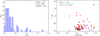 |
Fig. 9 Standard deviation ofσR5 for the GAPS transiting planet hosts:. Left panel: distribution of σR5. Right panel: standard deviation of R5 versus the |

GAPS transiting systems with σR5 > 0.5.
6.1 Comparison with MS and evolved stars
To put the activity of host stars into context, we exploited the sample composed by Pace (2013) with a compilation of S-index measurements for about 2000 field stars from the literature. To remain homogeneous with the planetary host data, we search each field star in Gaia DR3 and eventually we evaluate the (B–V) color and the temperature for each star in the same way as described in Sect. 3. Since MS and evolved stars have very different activity distributions (Wright 2004; Mittag et al. 2013; Staab et al. 2017), to separate them in the field star sample, we used the absolute magnitude obtained from the XHIP catalog (Anderson & Francis 2012) and built an HR diagram (Fig. 11) using the average MS defined by Wright (2004) as in Sect. 3.
We computed the  values for both the MS and evolved stars identified in the Pace (2013) sample, following the procedure described in Sect. 4.2. The two left panels of Fig. 12 show the
  measurements for the planetary hosts compared with MS field stars (top panels) or evolved stars (bottom panels). In the top left panel, the basal limit for MS stars is also indicated with a horizontal black line. The basal level of activity is the stellar analog of the quiet Sun reached by stars with no chromospherically active regions (e.g., Schrijver 1987; Schröder et al. 2012). The basal activity limit of
  is applied only for dwarfs with solar metallicity. It is a little bit different (−5.15) for MS stars with super-solar metallicity (Henry et al. 1996; Wright 2004; Saar 2011). Furthermore, the basal level is also a slightly complicate function of the (B–V) of the star (Mittag et al. 2013, and references therein). Considering the polynomial model of the basal level described in Table 3 of Mittag et al. (2013), we superimposed it (the blue dashed curve) on the top-left panel of Fig. 12. The largest difference between the two descriptions of the basal level is visible in the red portion of the plot where the model has a quadratic dependence on the B–V color. The presence of a relative maximum in the range 1.1 < B − V ≤ 1.45 has been justified by Mittag et al. (2013) with the absence of inactive stars in that color range. Instead, in the bluer range of the diagram, the difference between the two is inside the median measurement error. In any case, the polynomial description does not represent the basal limit in a better way than a constant value of −5.1 (e.g. Henry et al. 1996; Wright 2004; Staab et al. 2017; Haswell et al. 2020).
The right panels of Fig. 12 compare the histogram and cumulative distribution function of  for both the host and MS stars (top – right), and for host and slightly evolved stars (bottom – right). A comparison of the hosts with MS and evolved star populations shows that they actually come from different parent distributions in both cases (see Appendix B). This difference can be interpreted as due to observational selection biases that make planet detection more likely for less active hosts.
Among the MS stars in Pace (2013), there are very few stars (about 0.3%) below the basal activity level of -5.1, and about 1% in the complete sample. In our sample of transiting -planet hosts, ten stars (CoRoT-1, GJ436, HAT-P-35, HAT-P-44, HAT-P-45, HAT-P-46, Kepler-25, WASP-12, WASP-18, WASP-72), corresponding to 8% of our sample, show activity levels below the basal limit. Two of these, WASP-12, and WASP-72, are reported to be sub-giants having the ∆MV > 0.45 (0.74, and 1.26, respectively, see Sect. 3)8. Evolved stars can be inactive stars well below the basal limit for MS stars (e.g., Wright 2004). The remaining host stars are all MS stars and in those cases, a mechanism that suppresses the star activity, making it lower than the basal limit should be at work. The activity suppression seems more common in our sample of planet-transiting hosts than in the field stars. This mechanism could also veil the CE of more active stars, but in this case, it will be very difficult to identify it. Hence, the activity suppression due to evaporated shrouds could be a more common phenomenon than it appears.
The presence of some planetary hosts below the MS activity basal limit has been interpreted as an indication that the presence of short-period massive planets mimics an activity suppression, but it is actually due to circumstellar absorption linked to planetary mass loss, which is sensitive to the surface gravity of the planet (Lanza 2014; Fossati et al. 2015). The same behavior of some MS stars has been considered, with success, which is indicative of undiscovered mass-losing planets (Haswell et al. 2020). A model that reproduces the observed correlation was proposed by Lanza (2014) and Fossati et al. (2015). On the other hand, since the transiting planet hosts are also distant stars (see the upper panel of Fig. 2 for the sample under study), a contribution to this suppression of the observed chromospheric index may be also given by the interstellar medium (Staab et al. 2017).
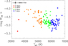 |
Fig. 10 Values of |


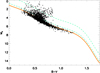 |
Fig. 11 HR Diagram for the field stars in the Pace (2013) sample. The HIPPARCOS average MS by Wright (2004) and the loci 0.45 and 2 mag above it are indicated in orange and green, as in Fig. 6. |
6.2 Considering whether the ISM absorption could bias the chromospheric activity level
The value of  of 8% of our sample of stars is lower than the activity basal limit for the MS. One of the causes that can contribute to justifying this low value of the
  is the possible absorption of the HK flux by the interstellar medium (ISM).
Figure 13 shows the distribution of the transit hosts into the Galaxy. The red stars indicate the line of view of the hosts with an activity level lower than the basal one. In the plot, there is no evidence of a preferred direction. As we saw in Sect. 3, most of the stars we are considering have distances greater than 100 pc. For these systems, the ISM absorption has a significant influence on the measurement of the activity. As a matter of fact, beyond 100 pc the column density of the ISM Ca II is about 1012 cm−2 (Welsh et al. 2010; Wyman & Redfield 2013; Fossati et al. 2017).
Following the work of Fossati et al. (2017), for each target we evaluate the column density of ISM Ca II. We utilized the ISM maps by Lallement et al. (2019, 2022) to evaluate E(B-V) and successively the relation by Diplas & Savage (1994) to derive the column density of H I. The relation between the NH I and the ionic gas-phase abundance of ISM by Wakker & Mathis (2000) gave us the column density of Ca II. Finally, to obtain the correction of the  for the ISM absorption, we used the IDL procedure CORRECTION. PRO, described by Fossati et al. (2017, more details are given in Table A.2).
We note that with the only exception of HAT-P-44 and HAT-P-45, all the other eight MS systems with  ≤ −5.1 remain below the basal level after the application of the correction (see the systems highlighted in Table A.2). We can conclude that for these systems, the ISM absorption only partially explains the suppression of the CA index below the basal level, so that other mechanisms, such as absorption from evaporated shrouds, are at work.
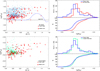 |
Fig. 12 Comparison of the CA of host stars with the CA of MS and evolved stars. Top panel: distribution of the MS-field stars with ∆MV ≤ 0.45 above the average HIPPARCOS MS (cyano small filled circles) and the transiting planet hosts (left). In the plot, we also indicated two representations of the activity basal limit for MS stars. The black dashed line is the generally considered constant limit. The blue dashed line is the polynomial model of the basal level (Mittag et al. 2013). The comparison of the normalized histograms and the cumulative distribution functions of the two distributions in the left panel (right). Bottom panel: evolved field stars with 0.45 ≤ ∆MV ≤ 2.00 above the average Hypparcos MS (small filled green circles) and the transiting planet hosts (of both samples) are on the left. A comparison of the normalized histograms and the cumulative distribution functions of the two distributions in the left panel is on the right. |
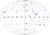 |
Fig. 13 Aitoff projection of the distribution of transit hosts in our sample in Galactic coordinates l and b of sight lines. The Galactic center is located at the center of the plot and the longitude increases counterclockwise. In the plot, the hosts with |

7 Host activity and planetary parameters analysis
We searched for correlations between the  and planetary parameters, such as the mass (MP), the radius (RP), the density (ρP), and the orbital distance (aP) of the planets. We checked also for correlation of the activity level with the planet’s insolation (S⋆ /S0; S0 is the Earth’s insolation at the top of the atmosphere), the equilibrium temperature (Teq,P) of the planet assuming zero bond albedo. Considering also the star-planet interaction (SPI), we take into account the possibility that tidal interaction between the planet and its star can generate an enhancement of local turbulent velocity, resulting in an increment of the heating and a rise in stellar activity level (Cuntz et al. 2000). Hence, we searched for a correlation with the stellar gravitational perturbation by the planet (Cuntz et al. 2000):

where MP, M⋆, and R⋆ are the mass of the planet, the mass of the star, and the radius of the star, respectively; 𝑔⋆ is the surface gravity of the host star, and ap is the orbital axis of the planet.
While the former set of variables consists of planetary quantities, the latter set contains quantities evaluated with both star and planet parameters. We used planetary data determined in a previous work (Bonomo et al. 2017), while for planets in our sample not considered in that work, we used the Exoplanet Ency-clopaedia9 (Schneider et al. 2011), searching the literature, to obtain the mass, and radius and all the other useful parameters (aP, log(𝑔P), etc.). We are aware that the derivation of the planetary parameters obtained in this way has a degree of inho-mogeneity, which can produce biased results, and we stress that the investigation that follows should be seen with this caveat in mind.
The analysis of all the possible correlations has been performed using the Spearman’s rank coefficient (Press et al. 1992), as was already done on smaller samples of transiting planets by Hartman (2010) and Figueira et al. (2014). For each correlation coefficient, we obtained the false alarm probability (FAP) or the probability of having a larger or equal correlation coefficient under the hypothesis that the data pairs are uncorrelated (our null hypothesis). The tests were performed considering the whole sample of host-planet pairs with no restrictions and a second sub-set responding to the condition: ap ≤ 0.1, and Mp ≥ 0.1 MJ. In Table 4, we summarize the results.
Among the planetary parameters, the correlation between  and MP has a value of Spearman’s correlation coefficient that is not different from zero with a FAP of 73% considering the whole sample. This seems to contradict the statistical explanation of Collier Cameron & Jardine (2018) of the correlation reported by Hartman (2010) and Figueira et al. (2014) between the CE and the surface gravity of close-orbiting planets based on the statistical bias towards younger systems produced by the faster inward migration of more massive planets because of their stronger tidal interaction with their host stars. The correlation with the orbital semi-major axis aP has a FAP = 4%. This is the only SPI correlation that has been considered so far by further dedicated studies (e.g. Figueira et al. 2014), to the best knowledge of the authors. Instead, the correlation with the RP (FAP= 1.0% and FAP = 0.09%) have a confidence level greater than 99%, while log 𝑔P (FAP = 1.5% whole sample and 2.3% the limited one), and the density of the planet pP (FAP = 3% and FAP = 0.7%), have all a confidence in the range between 97% and 99%.
Concerning the parameter containing stellar and planetary quantities, the correlation with insolation S⋆/S0, and the planetary Teq,P show also a confidence greater than 99%. This is not the same result, however, for the quantity ∆𝑔⋆/𝑔⋆ (FAP = 94% and 63%). In Fig. 14, we reported the value of  of the object as a function of the ratio, η, between the semi-major axis, ap, of the planet and the value of the Roche limit of the system (Faber et al. 2005; Ford & Rasio 2006):
 (7)
(7)
where aRoche is the critical separation at which the planet fills its Roche’s lobe and it begins to lose mass. This limit is a function of the planetary radius Rp, and of the stellar (M⋆) and planetary (MP) masses.
The analysis of the correlation between η and  does not give a significant correlation (Fig. 14). The Spearman’s rank coefficient results ρ = 0.02 with a FAP ~ 83%, but it is worth noting that all the hosts with
  lower than the basal limit have planets with a mean density (1.7×10³ kg m−3) that is lower than the average density (2.2×10³ kg m−3) of the planets with the ratio η in the interval [1 , 10]. Actually, in the same range of η values, there is a high spread in the activity level of the hosts. The spread could be due to the dispersion of the host age and/or to the spread of the planetary companions’ densities. In fact, in both cases, they are the stellar and planetary parameters with higher standard deviations by their mean values. There is not a clear indication of which parameter can account for it. Another reason that accounts for the spread in this region of the plot could be the presence of matter evaporated by the planet that, depending on its quantity, could veil (with different levels of efficiency) the CE of the stars.
In the region of the plot for η > 10, the distribution of the activity levels has a reduced spread, and it is possible to define a border-line  that separates the space in the diagram between a region that is populated by the hosts of transiting planets and one that is empty. Because we are considering only transiting planets, the population of the η > 10 zone in the
  plane could be the result of a selection effect. Planets observed with the RV method (e.g., the sample discussed by Canto Martins et al. 2011) could help to populate this zone and unveil whether there is a selection effect present. For those planets, the value of the radius is unknown and the mass obtained is the minimum mass, making it impossible to evaluate the η value for those systems using measured quantities.
To conclude this section, we can say that there is no evidence for a strong single correlation between the activity level of the planet host star and one of the planetary and stellar parameters. Instead, a slight correlation seems to arise when we considered planetary parameters depending on the radius of the planet (surface gravity, density, insolation). All the parameters that have a correlation with  with a confidence value greater than 98% are
  suggesting a common origin. The same is true for the insolation and the Teq,P that show a negative correlation with the activity. The analysis of these correlations confirms that close-in transiting planets swell under the irradiation from their host stars corroborating the hypothesis already discussed in preceding works (e.g., Lanza 2014; Fossati et al. 2013, 2015) that the planetary atmosphere evaporates under the action of the stellar irradiation and the matter lost by the planet forms shrouds that absorb at the core of the chromospheric resonance lines (e.g., Mg II h&k, Ca II H&K), making the observed chromospheric emission correspondingly lower. Due to the role of the planetary radius in these correlations, the mechanism at work could be the hydrodynamic escape to which some of these planets (those with the
  lower than the basal value) should be subject. In this direction, we get also an indication that hosts with
  lower than the basal limit for MS stars are very close to filling their Roche lobe even if other unknown phenomena could have their effects.
On the other hand, it is worth noting that the analyzed correlations with the possible star-planet interaction (aP and ∆𝑔★ + 𝑔★) are not significant ones. This seems to indicate that the higher activity level of some of the considered transit hosts in this study is not due to the SPI, but it appears natural.
Statistical analysis of the correlation between the CA indicator <  > and different planetary parameters of the transiting planetary systems.
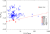 |
Fig. 14 Activity level as a function of the ratio η between the semi-major axis and the Roche lobe radius. The hosts with |

8 Machine learning classification
In order to test the Lanza (2014) model of planetary material absorbing at the core of chromospheric resonance lines, Fossati et al. (2015) applied a cluster-weighted model (Ingrassia et al. 2012) to distinguish different sub-populations in their data. This model reproduces the bimodal distribution observed in the CA level of solar-like stars in the field, the so-called Vaughan-Preston gap (e.g., Wright 2004). Specifically, the existence of two linear regressions can be considered to be the natural outcome of the underlying bimodal distribution of the chromospheric index. These authors explored the likelihood of one to three components in their data set and found two components to be the most likely representation.
Following these results, we also classified our data based on the  and the inverse of the planetary surface gravity,
  . In this analysis, we only considered systems with main sequence stars and excluded those with an eccentric orbit and planetary masses in the Neptunian range. For the latter, in particular, there would not be enough planetary material available to create the absorbing torus predicted by Lanza (2014). Moreover, as the effect of planetary material on stellar chromospheric lines is only expected for close-in planets, we excluded systems with ap > 0.1 AU.
Our data set is larger than that of Fossati et al. (2015)’s by almost a factor of 3, and we visually identified four possible components: the same high- and low-activity components they highlighted, a third component with average activity and high inverse of the surface gravity  , namely, low planetary-surface gravity and a high-activity component with low correlation with
  . We hypothesize the third population might represent a “saturated” regime for stellar irradiation-driven planet evaporation, where planetary mass loss
  becomes proportional to the square root of the stellar UV flux (Murray-Clay et al. 2009), rather than being proportional to the UV flux as assumed in the energy-limited evaporation model by Lanza (2014). Therefore, for this subset, a lower evaporation rate for a given
  than assumed by Lanza (2014) would hold and this would imply a lower absorption by the evaporated matter than predicted by his model. The fourth population might instead represent a set of stars with an intrinsically high level of activity and a strong enough stellar wind to blow away all evaporated matter, making the measured stellar chromospheric emission virtually unaffected by planet evaporation.
In light of the already available information, as well as our aforementioned hypotheses, we implemented a supervised machine-learning classification scheme to determine a statistically-motivated separation between the subsets. The details of its training and implementation can be found in Appendix C. This resulted in the grouping presented in Fig. 15, where each data point is represented by a marker and colour corresponding to its predicted cluster membership, and where white-filled data points are those with an assignment probability <70%: a similar threshold was used by Fossati et al. (2015) to identify points that might likely belong to a different cluster. The high- and low-activity, low  populations (recalling those of Fossati et al. 2015) were then used to carry out linear fits in the
  space, following the Lanza (2014) model. This required including the data point uncertainties both in the classification and fits: to do this, we first conservatively expanded the error bars of the high-activity systems
  to 0.25 dex, based on the values shown in Fig. 3 of Wright (2004). This allowed us to take into account realistic variations due to the activity cycle. We then bootstrapped our data set 1000 times, on the basis of each data point’s Gaussian uncertainty in
  . At every iteration, the previously-trained classification was carried out on the new data set, and linear fits were performed on the synthetic data set. For every realization, we only considered points with a >70% probability of being assigned to a given cluster, to then fit the populations with the linear model
  . We obtained:
γ = −336.16 ± 181.66,
 for the high-activity cluster;
γ = −54.26 ± 44.56,
 for the low-activity cluster.
Both populations are in 3σ agreement with Fossati et al. (2015): the parameter space investigated by these authors and the trends they identified are shown in Fig. 15. The γ coefficients of both populations are, however, less significant than those found by Fossati et al., while the one on the high-activity population is more significant than the one found by Danielski et al. (2022). Such differences might relate to different factors, such as the kind of classification algorithm, the details of the conversion between the S and the  activity indexes, and, most importantly, the size of the sample. All are aspects that play a key role in the classification process and identified correlations. Another relevant aspect is the probability of assignment to the high- or low-activity cluster or even to the high-activity and higher
  group, of single data points. For these reasons, we highlight the need to perform further investigations which use a larger homogeneous sample, to shed light on how planetary systems populate this parameter space. This might reduce the reliance on training information and allow for the use of unsupervised algorithms to increase the robustness of the clustering and, therefore, the estimates of the correlation coefficients.
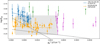 |
Fig. 15 Clustering in the |


9 Summary and conclusions
In this work, we have presented the characterization of a part of the hosts of transiting planets of the GAPS sample, mainly analyzing their stellar chromospheric activity (CA). In the process, we added to the observed data others found in the literature obtained for other hosts of transiting planets, enlarging the data set on which the cited previous works were based.
For each of the 132 stars in the sample, we obtained the stellar parameters (Teff, B–V, V in a homogeneous way, exploiting the Gaia DR3 data release (Gaia Collaboration 20l6, 2018, 2023). Subsequently, the complete set was compared with the activity levels of the field stars. To do this, we used the Mittag et al. (2013) procedure for calculating  values. We report an activity index between −5.373 and −3.972, with a median value of −4.810. Somewhat more than half of the sample (58%) are inactive stars and this was expected, as most of our sample was selected from radial velocity follow-up campaigns, which privilege inactive stellar hosts. This study allowed us to determine a relationship between the
  values calculated with the classical procedure (Noyes et al. 1984) and those obtainable with Mittag’s procedure, in the event that the S-index value is not available for the given object. This relationship has been determined both for MS and slightly evolved objects.
The analysis of the time series of  for the GAPS objects observed for more than 20 nights showed that some of the targets have a dispersion value σR5 > 0.5 dex. In one case, Qatar-2, the high dispersion value (1.736 dex) and the low time-lapse of the time series seem to indicate a flare event. In general, as expected, the activity dispersion pattern is proportional to the activity level of the star, but in the cases of the F stars WASP-1, HAT-P-16, XO-4, and in that of the K star HAT-P-26, although these stars have a
  value included in the zone of inactive stars
  , they show a large variation in activity. This behavior confirms the high activity variation for K and F stars with low activity levels observed by Gomes da Silva et al. (2021).
We contrasted also the transiting planet hosts (both GAPS and those taken from the literature) with the field objects of both MS and slightly evolved by Pace (2013) after that we obtained also for field stars the stellar parameters by Gaia/DR3 in order to compare homogeneous samples. Kolmogorov-Smirnov tests show that the population of transiting objects is different from both populations (stars of MS and sub-giants) of the field objects. In addition, the population of transiting objects shows a higher percentage of objects (8% of the sample corresponding to 11 stars) with an activity level lower than the basal activity level for main sequence stars than in the case of field objects (1%). While three of these objects are subgiants, the other eight are stars of MS, for which there is a process of suppression of chromospheric line core fluxes that we have ascertained not to be due to the interstellar medium.
We analyzed the presence or the absence of possible correlations between the level of CA of the host stars and the stellar and planetary parameters of the systems considered. In particular, we tested the correlations of the activity level with the following planetary parameters: MP, RP, log 𝑔P, ρP and aP, the insolation at the top of the planet’s atmosphere, the Teą,p, the equilibrium temperature of the planet and the stellar equilibrium tide. The analysis has been performed for the whole sample and for a limited sub-set to MP ≥ 0.1MJ and ap ≤ 0.1 au. We did not find significant correlations with aP, the only planetary parameter linked to the existence of star-planet interaction. Furthermore, the lack of a correlation with MP seems to contradict the Collier Cameron & Jardine (2018)’s explanation of the correlation firstly reported by Hartman (2010). Conversely, all correlations with FAP ≤ 1% are with planetary parameters proportional to  , indicating a common origin. We conclude that some planets evaporate by means of hydrodynamic escape under the strong irradiation of the host star and the evaporated matter forms a system of shrouds that absorbs the core of chromospheric resonance lines, as described by Lanza (2014). This is confirmed by the fact that all the systems with activity lower than the basal level host planets that are very close to filling their Roche lobe.
An analysis made with a machine learning technique supported the presence of four different clusters of hosts with different behavior concerning the activity of stars as a function of the planetary surface gravity. Two of these clusters were already individuated by Fossati et al. (2015). The third cluster, with average activity and low planetary surface gravity, has been interpreted as due to a “saturated” regime for stellar irradiation-driven evaporation. The fourth cluster likely represents stars with a high level of activity and a strong stellar wind able to remove the shrouds of evaporated matter. So far, these interpretations are qualitative ones and they are the subject of ongoing and future works.
Acknowledgements
The authors are greateful to an anonymous referee for a careful reading of the manuscript and a very useful report that helped them to remarkably improve their work and its presentation. The GAPS project in Italy acknowledges the support by INAF through the Progetti Premiali funding scheme of the Italian Ministry of Education, University, and Research. Based on observations made with the Italian Telescopio Nazionale Galileo (TNG) operated on the island of La Palma by the Fundacion Galileo Galilei of the INAF (Istituto Nazionale di Astrofisica) at the Spanish Observatorio del Roque de los Muchachos of the Instituto de Astrofisica de Canarias This research has made use of the VizieR catalog access tool, CDS, Strasbourg, France (DOI: 10.26093/cds/vizier) and of SIMBAD database, operated at CDS, Strasbourg, France. This work has made use of data from the European Space Agency (ESA) mission Gaia (https://www.cosmos.esa.int/gaia), processed by the Gaia Data Processing and Analysis Consortium (DPAC, https://www.cosmos.esa.int/web/gaia/dpac/consortium). Funding for the DPAC has been provided by national institutions, in particular, the institutions participating in the Gaia Multilateral Agreement.
Appendix A Additional tables
Journal of GAPS Observations.
Correction  and corrected value of
  for the ISM absorption for the systems of the sample. The highlighted systems have still
  .
.
Appendix B Comparison between CA index distributions of field and transit host stars
The comparison of the four statistical moments of each distribution (see Table B.1) reveals that all are leptokurtic (kurt(X) > 0), and asymmetric distributions towards the higher values of  (skew(X)>0). In this contest, the host stars are more dispersed with respect to field stars, including both M-S and evolved field stars (σhost > σall > σM-S > σsub-giant). On the contrary, the host stars distribution is more symmetric with respect to the others (kurthost < kurtM-S < kurtall < kurtsub-giant).
Comparison of the values of the distribution moments of the different populations of objects.
A Kolmogorov-Smirnov test yields very low probabilities for the null hypothesis: the probability that the CA distributions for M-S field stars and planet hosts are drawn from the same parent population (Figure 12 top-right panel) is Prob = 1.29 × 10⁻¹³ (D=0.35, Ne = 120), while for evolved stars (Figure 12 bottom-right panel) we found Prob = 4.4 × 10⁻² (D=0.1, Ne = 103). Considering instead the whole distributions for field stars and planet hosts, we obtained Prob = 4.14 × 10⁻⁹ (D=0.3, Ne = 122) that they are drawn from the same parent population. It is worth noting that the field stars’ bimodality indicated by the different average values of  for M-S (−4.5862) and sub-giant (−4.7307), is expected (Wright 2004; Gray et al. 2006). In conclusion, the M-S and evolved stars’ CA distribution comes from a different parent distribution of the transit host stars.
Appendix C Details of machine learning analysis
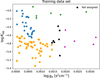 |
Fig. C.1 Training clustering provided to the algorithm in the |

In machine learning investigations, data points are represented by vectors containing different “features”, and classification methods divide n-dimensional samples into clusters according to different possible metrics. Another fundamental distinction is between unsupervised and supervised methods: the former do not rely on prior, or “training”, information, contrarily to the latter. Following Fossati et al. (2015), we first attempted a classification without prior information and assumed our data set could be represented by a finite number of Gaussian distributions. As shown by Danielski et al. (2022), this can be done with a Gaussian Mixture Model (GMM, Sorenson & Alspach 1971; Alspach & Sorenson 1972).
Before running the classification, we prepared our data set by normalizing it, in order to assign equal weight to each feature. This is usually done by removing the data mean and by scaling it to unit variance:
 (C.1)
(C.1)
where Z is the transformed data set, X is the raw data set, and µ and σ are its mean and standard deviation across every feature or parameter.
Then we adopted the GMM implementation in SCIKIT-LEARN (Pedregosa et al. 2011) and tested it by imposing an increasing number of sub-clusters. Even if the GMM was able to reproduce Fossati et al. (2015)’s result, we noticed its tendency to prefer three mixtures on our larger data set, where the entire sample of Fossati et al. (2015) is included in a single cluster. This can probably be explained by the different way clusters are formed by a GMM and by the cluster-weighted model adopted in their study. While in the former case, the data points are assumed to populate the  parameter space according to a number of multivariate Gaussian distributions, each with a center and a covariance matrix, the latter associates them to linear relationships following Lanza (2014)’s model.
We then preferred to use a supervised learning algorithm. After testing several algorithms, we chose a Decision Tree approach, which learns information from data using simple decision rules (e.g. Geron 2017). Once again, we relied on SCIKIT-LEARN’s implementation of this algorithm and chose a maximum depth of 4, that is, the one that allowed us to reproduce a close clustering to the one of Fossati et al. (2015)’s on their data.
We trained the algorithm after visual inspection on how four clusters might be identified in the data set (see Sect. 8 in the main text). We assigned 94% of the data point to different clusters, as shown by the colours used in Figure C.1, leaving out a few points at the edge of the clusters. A cross-validation test (e.g. Geron 2017) yielded an accuracy of (91 ± 6)% for our combination of algorithms and training data. Then, we ran the Decision Tree on the whole data set and obtained the classification shown in Figure 15 in the main text. We remark that we could not use a classical “score test” to measure the accuracy of the prediction, as we worked in a framework of multi-label, and not binary, classification (see SCIKIT-LEARN’s documentation of the Decision Tree algorithm).
References
- Albrecht, S., Winn, J. N., Butler, R. P., et al. 2012, ApJ, 744, 189 [NASA ADS] [CrossRef] [Google Scholar]
- Alspach, D., & Sorenson, H. 1972, IEEE Trans. Automatic Control, 17, 439 [CrossRef] [Google Scholar]
- Anderson, E., & Francis, C. 2012, Astron. Lett., 38, 331 [Google Scholar]
- Anderson, D. R., Collier Cameron, A., Gillon, M., et al. 2011, A&A, 534, A16 [NASA ADS] [CrossRef] [EDP Sciences] [Google Scholar]
- Anderson, D. R., Collier Cameron, A., Delrez, L., et al. 2014, MNRAS, 445, 1114 [NASA ADS] [CrossRef] [Google Scholar]
- Bailer-Jones, C. A. L., Rybizki, J., Fouesneau, M., Demleitner, M., & Andrae, R. 2021, AJ, 161, 147 [Google Scholar]
- Bailey, A., & Goodman, J. 2019, MNRAS, 482, 1872 [NASA ADS] [CrossRef] [Google Scholar]
- Bakos, G. Á., Hartman, J. D., Torres, G., et al. 2012, AJ, 144, 19 [NASA ADS] [CrossRef] [Google Scholar]
- Baliunas, S. L., Donahue, R. A., Soon, W. H., et al. 1995, ApJ, 438, 269 [Google Scholar]
- Ballerini, P., Micela, G., Lanza, A. F., & Pagano, I. 2012, A&A, 539, A140 [NASA ADS] [CrossRef] [EDP Sciences] [Google Scholar]
- Barclay, T., Kostov, V. B., Colón, K. D., et al. 2021, AJ, 162, 300 [NASA ADS] [CrossRef] [Google Scholar]
- Barker, A. J. 2020, MNRAS, 498, 2270 [Google Scholar]
- Bastian, T. S., Dulk, G. A., & Leblanc, Y. 2000, ApJ, 545, 1058 [NASA ADS] [CrossRef] [Google Scholar]
- Beck, P. G., Kambe, E., Hillen, M., et al. 2015, A&A, 573, A138 [NASA ADS] [CrossRef] [EDP Sciences] [Google Scholar]
- Béky, B., Bakos, G. Á., Hartman, J., et al. 2011, ApJ, 734, 109 [CrossRef] [Google Scholar]
- Benatti, S. 2021, in Posters from the TESS Science Conference II (TSC2), 21 [Google Scholar]
- Biazzo, K., D’Orazi, V., Desidera, S., et al. 2022, A&A, 664, A161 [NASA ADS] [CrossRef] [EDP Sciences] [Google Scholar]
- Bonomo, A. S., Hébrard, G., Santerne, A., et al. 2012, A&A, 538, A96 [NASA ADS] [CrossRef] [EDP Sciences] [Google Scholar]
- Bonomo, A. S., Desidera, S., Benatti, S., et al. 2017, A&A, 602, A107 [NASA ADS] [CrossRef] [EDP Sciences] [Google Scholar]
- Borsa, F., Rainer, M., Bonomo, A. S., et al. 2019, A&A, 631, A34 [NASA ADS] [CrossRef] [EDP Sciences] [Google Scholar]
- Borucki, W. J., Koch, D. G., Batalha, N., et al. 2012, ApJ, 745, 120 [NASA ADS] [CrossRef] [Google Scholar]
- Borucki, W. J., Agol, E., Fressin, F., et al. 2013, Science, 340, 587 [NASA ADS] [CrossRef] [Google Scholar]
- Bressan, A., Marigo, P., Girardi, L., et al. 2012, MNRAS, 427, 127 [NASA ADS] [CrossRef] [Google Scholar]
- Brown, D. J. A., Cameron, A. C., Anderson, D. R., et al. 2012, MNRAS, 423, 1503 [NASA ADS] [CrossRef] [Google Scholar]
- Buchhave, L. A., Bakos, G. Á., Hartman, J. D., et al. 2011, ApJ, 733, 116 [NASA ADS] [CrossRef] [Google Scholar]
- Canto Martins, B. L., Das Chagas, M. L., Alves, S., et al. 2011, A&A, 530, A73 [NASA ADS] [CrossRef] [EDP Sciences] [Google Scholar]
- Carleo, I., Benatti, S., Lanza, A. F., et al. 2018, A&A, 613, A50 [NASA ADS] [CrossRef] [EDP Sciences] [Google Scholar]
- Carleo, I., Malavolta, L., Lanza, A. F., et al. 2020, A&A, 638, A5 [NASA ADS] [CrossRef] [EDP Sciences] [Google Scholar]
- Carleo, I., Giacobbe, P., Guilluy, G., et al. 2022, AJ, 164, 101 [NASA ADS] [CrossRef] [Google Scholar]
- Cegla, H. M., Watson, C. A., Shelyag, S., et al. 2018, ApJ, 866, 55 [NASA ADS] [CrossRef] [Google Scholar]
- Claudi, R., Benatti, S., Carleo, I., et al. 2016, SPIE Conf. Ser., 9908, 99081A [NASA ADS] [Google Scholar]
- Claudi, R., Benatti, S., Carleo, I., et al. 2017, Eur. Phys. J. Plus, 132, 364 [NASA ADS] [CrossRef] [Google Scholar]
- Collier Cameron, A., & Jardine, M. 2018, MNRAS, 476, 2542 [Google Scholar]
- Cosentino, R., Lovis, C., Pepe, F., et al. 2012, SPIE Conf. Ser., 8446, 84461V [Google Scholar]
- Covino, E., Esposito, M., Barbieri, M., et al. 2013, A&A, 554, A28 [NASA ADS] [CrossRef] [EDP Sciences] [Google Scholar]
- Cuntz, M., Saar, S. H., & Musielak, Z. E. 2000, ApJ, 533, L151 [Google Scholar]
- da Silva, L., Girardi, L., Pasquini, L., et al. 2006, A&A, 458, 609 [NASA ADS] [CrossRef] [EDP Sciences] [Google Scholar]
- Damasso, M., Lanza, A. F., Benatti, S., et al. 2020, A&A, 642, A133 [EDP Sciences] [Google Scholar]
- Danielski, C., Brucalassi, A., Benatti, S., et al. 2022, Exp. Astron., 53, 473 [NASA ADS] [CrossRef] [Google Scholar]
- Diplas, A., & Savage, B. D. 1994, ApJ, 427, 274 [Google Scholar]
- Dumusque, X., Bonomo, A. S., Haywood, R. D., et al. 2014, ApJ, 789, 154 [NASA ADS] [CrossRef] [Google Scholar]
- Duncan, D. K., Vaughan, A. H., Wilson, O. C., et al. 1991, ApJS, 76, 383 [Google Scholar]
- Egeland, R., Soon, W., Baliunas, S., et al. 2017, ApJ, 835, 25 [NASA ADS] [CrossRef] [Google Scholar]
- Esposito, M., Covino, E., Desidera, S., et al. 2017, A&A, 601, A53 [NASA ADS] [CrossRef] [EDP Sciences] [Google Scholar]
- Evans, D. W., Riello, M., De Angeli, F., et al. 2018, A&A, 616, A4 [NASA ADS] [CrossRef] [EDP Sciences] [Google Scholar]
- Faber, J. A., Rasio, F. A., & Willems, B. 2005, Icarus, 175, 248 [NASA ADS] [CrossRef] [Google Scholar]
- Figueira, P., Oshagh, M., Adibekyan, V. Z., & Santos, N. C. 2014, A&A, 572, A51 [NASA ADS] [CrossRef] [EDP Sciences] [Google Scholar]
- Ford, E. B., & Rasio, F. A. 2006, ApJ, 638, L45 [Google Scholar]
- Fossati, L., Haswell, C. A., Froning, C. S., et al. 2010, ApJ, 714, L222 [Google Scholar]
- Fossati, L., Ayres, T. R., Haswell, C. A., et al. 2013, ApJ, 766, L20 [Google Scholar]
- Fossati, L., Ingrassia, S., & Lanza, A. F. 2015, ApJ, 812, L35 [NASA ADS] [CrossRef] [Google Scholar]
- Fossati, L., Marcelja, S. E., Staab, D., et al. 2017, A&A, 601, A104 [NASA ADS] [CrossRef] [EDP Sciences] [Google Scholar]
- Gaia Collaboration (Prusti, T., et al.) 2016, A&A, 595, A1 [NASA ADS] [CrossRef] [EDP Sciences] [Google Scholar]
- Gaia Collaboration (Brown, A. G. A., et al.) 2018, A&A, 616, A1 [NASA ADS] [CrossRef] [EDP Sciences] [Google Scholar]
- Gaia Collaboration (Vallenari, A., et al.) 2023, A&A, 674, A1 [NASA ADS] [CrossRef] [EDP Sciences] [Google Scholar]
- Gautier, Thomas N., I., Charbonneau, D., Rowe, J. F., et al. 2012, ApJ, 749, 15 [NASA ADS] [CrossRef] [Google Scholar]
- Geron, A. 2017, Hands-on Machine Learning with Scikit-Learn and TensorFlow (Sebastopol, CA: O’Reilly Media, Inc.) [Google Scholar]
- Gilliland, R. L., Marcy, G. W., Rowe, J. F., et al. 2013, ApJ, 766, 40 [NASA ADS] [CrossRef] [Google Scholar]
- Gomes da Silva, J., Santos, N. C., Adibekyan, V., et al. 2021, A&A, 646, A77 [NASA ADS] [CrossRef] [EDP Sciences] [Google Scholar]
- Gray, R. O., Corbally, C. J., Garrison, R. F., et al. 2006, AJ, 132, 161 [Google Scholar]
- Guilluy, G., Andretta, V., Borsa, F., et al. 2020, A&A, 639, A49 [EDP Sciences] [Google Scholar]
- Gurdemir, L., Redfield, S., & Cuntz, M. 2012, PASA, 29, 141 [NASA ADS] [CrossRef] [Google Scholar]
- Hall, J. C., Lockwood, G. W., & Skiff, B. A. 2007, AJ, 133, 862 [Google Scholar]
- Hartman, J. D. 2010, ApJ, 717, L138 [NASA ADS] [CrossRef] [Google Scholar]
- Hartman, J. D., Bakos, G. Á., Torres, G., et al. 2011, ApJ, 742, 59 [NASA ADS] [CrossRef] [Google Scholar]
- Hartman, J. D., Bakos, G. Á., Béky, B., et al. 2012, AJ, 144, 139 [NASA ADS] [CrossRef] [Google Scholar]
- Hartman, J. D., Bakos, G. Á., Torres, G., et al. 2014, AJ, 147, 128 [NASA ADS] [CrossRef] [Google Scholar]
- Haswell, C. A., Fossati, L., Ayres, T., et al. 2012, ApJ, 760, 79 [Google Scholar]
- Haswell, C. A., Staab, D., Barnes, J. R., et al. 2020, Nat. Astron., 4, 408 [Google Scholar]
- Hatzes, A. P. 1996, PASP, 108, 839 [NASA ADS] [CrossRef] [Google Scholar]
- Hebb, L., Collier-Cameron, A., Loeillet, B., et al. 2009, ApJ, 693, 1920 [Google Scholar]
- Hébrard, G., Collier Cameron, A., Brown, D. J. A., et al. 2013, A&A, 549, A134 [NASA ADS] [CrossRef] [EDP Sciences] [Google Scholar]
- Henry, T. J., Soderblom, D. R., Donahue, R. A., & Baliunas, S. L. 1996, AJ, 111, 439 [Google Scholar]
- Howard, A. W., Johnson, J. A., Marcy, G. W., et al. 2011, ApJ, 730, 10 [NASA ADS] [CrossRef] [Google Scholar]
- Hunter, A. A., Macgregor, A. B., Szabo, T. O., Wellington, C. A., & Bellgard, M. I. 2012, Source Code Biol. Med., 7, 1 [Google Scholar]
- Ingrassia, S., Minotti, S. C., & Vittadini, G. 2012, J. Classif., 29, 363 [CrossRef] [Google Scholar]
- Kashyap, V. L., Drake, J. J., & Saar, S. H. 2008, ApJ, 687, 1339 [NASA ADS] [CrossRef] [Google Scholar]
- Knutson, H. A., Howard, A. W., & Isaacson, H. 2010, ApJ, 720, 1569 [NASA ADS] [CrossRef] [Google Scholar]
- Lallement, R., Babusiaux, C., Vergely, J. L., et al. 2019, A&A, 625, A135 [NASA ADS] [CrossRef] [EDP Sciences] [Google Scholar]
- Lallement, R., Vergely, J. L., Babusiaux, C., & Cox, N. L. J. 2022, A&A, 661, A147 [NASA ADS] [CrossRef] [EDP Sciences] [Google Scholar]
- Lammer, H., Selsis, F., Ribas, I., et al. 2003, ApJ, 598, L121 [Google Scholar]
- Lanza, A. F. 2014, A&A, 572, L6 [NASA ADS] [CrossRef] [EDP Sciences] [Google Scholar]
- Lecavelier des Étangs, A. 2007, A&A, 461, 1185 [CrossRef] [EDP Sciences] [Google Scholar]
- Lecavelier des Étangs, A., Vidal-Madjar, A., McConnell, J. C., & Hébrard, G. 2004, A&A, 418, L1 [NASA ADS] [CrossRef] [EDP Sciences] [Google Scholar]
- Lendl, M., Anderson, D. R., Collier-Cameron, A., et al. 2012, A&A, 544, A72 [NASA ADS] [CrossRef] [EDP Sciences] [Google Scholar]
- Lendl, M., Triaud, A. H. M. J., Anderson, D. R., et al. 2014, A&A, 568, A81 [NASA ADS] [CrossRef] [EDP Sciences] [Google Scholar]
- Locci, D., Cecchi-Pestellini, C., & Micela, G. 2019, A&A, 624, A101 [NASA ADS] [CrossRef] [EDP Sciences] [Google Scholar]
- Lovis, C., Dumusque, X., Santos, N. C., et al. 2011, arXiv e-prints [arXiv:1187.5325] [Google Scholar]
- Madhusudhan, N. 2019, ARA&A, 57, 617 [NASA ADS] [CrossRef] [Google Scholar]
- Maggio, A., Pillitteri, I., Scandariato, G., et al. 2015, ApJ, 811, L2 [NASA ADS] [CrossRef] [Google Scholar]
- Malavolta, L., Borsato, L., Granata, V., et al. 2017, AJ, 153, 224 [NASA ADS] [CrossRef] [Google Scholar]
- Maldonado, J., Scandariato, G., Stelzer, B., et al. 2017, A&A, 598, A27 [NASA ADS] [CrossRef] [EDP Sciences] [Google Scholar]
- Marcy, G. W., Isaacson, H., Howard, A. W., et al. 2014, ApJS, 210, 20 [NASA ADS] [CrossRef] [Google Scholar]
- Maxted, P. F. L., Anderson, D. R., Collier Cameron, A., et al. 2011, PASP, 123, 547 [NASA ADS] [CrossRef] [Google Scholar]
- Milbourne, T. W., Haywood, R. D., Phillips, D. F., et al. 2019, ApJ, 874, 107 [Google Scholar]
- Miller, B. P., Gallo, E., Wright, J. T., & Pearson, E. G. 2015, ApJ, 799, 163 [NASA ADS] [CrossRef] [Google Scholar]
- Mittag, M., Schmitt, J. H. M. M., & Schröder, K. P. 2013, A&A, 549, A117 [NASA ADS] [CrossRef] [EDP Sciences] [Google Scholar]
- Montalto, M., Piotto, G., Marrese, P. M., et al. 2021, A&A, 653, A98 [NASA ADS] [CrossRef] [EDP Sciences] [Google Scholar]
- Murray-Clay, R. A., Chiang, E. I., & Murray, N. 2009, ApJ, 693, 23 [Google Scholar]
- Nardiello, D., Malavolta, L., Desidera, S., et al. 2022, A&A, 664, A163 [NASA ADS] [CrossRef] [EDP Sciences] [Google Scholar]
- Noyes, R. W., Bakos, G. Á., Torres, G., et al. 2008, ApJ, 673, L79 [NASA ADS] [CrossRef] [Google Scholar]
- Noyes, R. W., Hartmann, L. W., Baliunas, S. L., Duncan, D. K., & Vaughan, A. H. 1984, ApJ, 279, 763 [Google Scholar]
- Ochsenbein, F., Bauer, P., & Marcout, J. 2000, A&AS, 143, 23 [NASA ADS] [CrossRef] [EDP Sciences] [Google Scholar]
- Pace, G. 2013, A&A, 551, L8 [NASA ADS] [CrossRef] [EDP Sciences] [Google Scholar]
- Pecaut, M. J., & Mamajek, E. E. 2013, ApJS, 208, 9 [Google Scholar]
- Pedregosa, F., Varoquaux, G., Gramfort, A., et al. 2011, J. Mach. Learn. Res., 12, 2825 [Google Scholar]
- Penz, T., Micela, G., & Lammer, H. 2008, A&A, 477, 309 [NASA ADS] [CrossRef] [EDP Sciences] [Google Scholar]
- Pepe, F., Mayor, M., Galland, F., et al. 2002, A&A, 388, 632 [NASA ADS] [CrossRef] [EDP Sciences] [Google Scholar]
- Pepe, F., Cameron, A. C., Latham, D. W., et al. 2013, Nature, 503, 377 [NASA ADS] [CrossRef] [Google Scholar]
- Pillitteri, I., Wolk, S. J., Lopez-Santiago, J., et al. 2014, ApJ, 785, 145 [NASA ADS] [CrossRef] [Google Scholar]
- Pino, L., Désert, J.-M., Brogi, M., et al. 2020, ApJ, 894, L27 [Google Scholar]
- Poppenhaeger, K., Robrade, J., & Schmitt, J. H. M. M. 2010, A&A, 515, A98 [NASA ADS] [CrossRef] [EDP Sciences] [Google Scholar]
- Poppenhaeger, K., & Schmitt, J. H. M. M. 2011, ApJ, 735, 59 [NASA ADS] [CrossRef] [Google Scholar]
- Press, W. H., Teukolsky, S. A., Vetterling, W. T., & Flannery, B. P. 1992, Numerical recipes in C. The art of scientific computing (Cambridge: University Press) [Google Scholar]
- Quinn, S. N., Bakos, G. Á., Hartman, J., et al. 2012, ApJ, 745, 80 [NASA ADS] [CrossRef] [Google Scholar]
- Riello, M., De Angeli, F., Evans, D. W., et al. 2021, A&A, 649, A3 [NASA ADS] [CrossRef] [EDP Sciences] [Google Scholar]
- Robertson, P., Roy, A., & Mahadevan, S. 2015, ApJ, 805, L22 [NASA ADS] [CrossRef] [Google Scholar]
- Saar, S. H. 2011, ASP Conf. Ser., 448, 1239 [NASA ADS] [Google Scholar]
- Saar, S. H., & Cuntz, M. 2001, MNRAS, 325, 55 [NASA ADS] [CrossRef] [Google Scholar]
- Santos, N. C., Sousa, S. G., Mortier, A., et al. 2013, A&A, 556, A150 [NASA ADS] [CrossRef] [EDP Sciences] [Google Scholar]
- Sanz-Forcada, J., Ribas, I., Micela, G., et al. 2010, A&A, 511, L8 [NASA ADS] [CrossRef] [EDP Sciences] [Google Scholar]
- Sanz-Forcada, J., Micela, G., Ribas, I., et al. 2011, A&A, 532, A6 [NASA ADS] [CrossRef] [EDP Sciences] [Google Scholar]
- Sato, B., Hartman, J. D., Bakos, G. Á., et al. 2012, PASJ, 64, 97 [NASA ADS] [Google Scholar]
- Scandariato, G., Maggio, A., Lanza, A. F., et al. 2013, A&A, 552, A7 [NASA ADS] [CrossRef] [EDP Sciences] [Google Scholar]
- Scandariato, G., Maldonado, J., Affer, L., et al. 2017, A&A, 598, A28 [NASA ADS] [CrossRef] [EDP Sciences] [Google Scholar]
- Scharf, C. A. 2010, ApJ, 722, 1547 [NASA ADS] [CrossRef] [Google Scholar]
- Schneider, J., Dedieu, C., Le Sidaner, P., Savalle, R., & Zolotukhin, I. 2011, A&A, 532, A79 [NASA ADS] [CrossRef] [EDP Sciences] [Google Scholar]
- Schrijver, C. J. 1987, A&A, 172, 111 [NASA ADS] [Google Scholar]
- Schröder, K. P., Mittag, M., Pérez Martínez, M. I., Cuntz, M., & Schmitt, J. H. M. M. 2012, A&A, 540, A130 [NASA ADS] [CrossRef] [EDP Sciences] [Google Scholar]
- Shkolnik, E., Walker, G. A. H., & Bohlender, D. A. 2003, ApJ, 597, 1092 [NASA ADS] [CrossRef] [Google Scholar]
- Shkolnik, E., Walker, G. A. H., Rucinski, S. M., Bohlender, D. A., & Davidge, T. J. 2005, AJ, 130, 799 [NASA ADS] [CrossRef] [Google Scholar]
- Shkolnik, E., Bohlender, D. A., Walker, G. A. H., & Collier Cameron, A. 2008, ApJ, 676, 628 [NASA ADS] [CrossRef] [Google Scholar]
- Sorenson, H., & Alspach, D. 1971, Automatica, 7, 465 [CrossRef] [Google Scholar]
- Sousa, S. G., Adibekyan, V., Delgado-Mena, E., et al. 2018, A&A, 620, A58 [NASA ADS] [CrossRef] [EDP Sciences] [Google Scholar]
- Sousa, S. G., Adibekyan, V., Delgado-Mena, E., et al. 2021, A&A, 656, A53 [NASA ADS] [CrossRef] [EDP Sciences] [Google Scholar]
- Staab, D., Haswell, C. A., Smith, G. D., et al. 2017, MNRAS, 466, 738 [NASA ADS] [CrossRef] [Google Scholar]
- Triaud, A. H. M. J., Collier Cameron, A., Queloz, D., et al. 2010, A&A, 524, A25 [NASA ADS] [CrossRef] [EDP Sciences] [Google Scholar]
- Triaud, A. H. M. J., Queloz, D., Hellier, C., et al. 2011, A&A, 531, A24 [NASA ADS] [CrossRef] [EDP Sciences] [Google Scholar]
- Tsantaki, M., Sousa, S. G., Santos, N. C., et al. 2014, A&A, 570, A80 [NASA ADS] [CrossRef] [EDP Sciences] [Google Scholar]
- Vaughan, A. H., & Preston, G. W. 1980, PASP, 92, 385 [Google Scholar]
- Wakker, B. P., & Mathis, J. S. 2000, ApJ, 544, L107 [CrossRef] [Google Scholar]
- Welsh, B. Y., Lallement, R., Vergely, J. L., & Raimond, S. 2010, A&A, 510, A54 [NASA ADS] [CrossRef] [EDP Sciences] [Google Scholar]
- Wenger, M., Ochsenbein, F., Egret, D., et al. 2000, A&AS, 143, 9 [NASA ADS] [CrossRef] [EDP Sciences] [Google Scholar]
- Winn, J. N., Albrecht, S., Johnson, J. A., et al. 2011, ApJ, 741, L1 [NASA ADS] [CrossRef] [Google Scholar]
- Wright, J. T. 2004, AJ, 128, 1273 [Google Scholar]
- Wright, J. T. 2005, PASP, 117, 657 [Google Scholar]
- Wright, J. T., Marcy, G. W., Butler, R. P., & Vogt, S. S. 2004, ApJS, 152, 261 [Google Scholar]
- Wyman, K., & Redfield, S. 2013, ApJ, 773, 96 [NASA ADS] [CrossRef] [Google Scholar]
- Zacharias, N., Finch, C. T., Girard, T. M., et al. 2012, VizieR Online Data Catalog: I/322A [Google Scholar]
Since mid-2016, the Fabry Perot lamp has been operative, replacing the ThAr lamp due to a sharp decrease in the lamp flux.
Using SIMBAD (Wenger et al. 2000) and VIZIER (Ochsenbein et al. 2000).
We note in passing that the classification of WASP-12 as a subgiant, that is supported by the modeling of our HARPS-N spectra, may account for the decay rate of the orbit of its transiting planet due to the dissipation of tidal inertial gravity waves excited by the planet inside the star. According to the present theory of dynamic tide, those waves have a sufficient dissipation rate only if the core of WASP-12 is radiative, as generally predicted by stellar structure models in the case of a subgiant, but not in the case of a MS star because the latter would have a convective core leading to a much smaller dissipation (e.g., Bailey & Goodman 2019; Barker 2020).
Accessible from http://exoplanet.eu/
All Tables
For all systems, the table lists Gaia DR3 id., and (B – V), and Teff obtained by Gaia Collaboration (2018) as explained in the text.
Statistical analysis of the correlation between the CA indicator < > and different planetary parameters of the transiting planetary systems.
Correction and corrected value of for the ISM absorption for the systems of the sample. The highlighted systems have still .
Comparison of the values of the distribution moments of the different populations of objects.
All Figures
|
Fig. 1 GAPS observations of transiting hosts considered in this work. Top: number of spectra per star of the GAPS sample of transiting hosts. Middle: number of observing nights per star. Bottom: S/N value per star. |
| In the text | |
|
Fig. 2 Distributions of the stellar parameters of the GAPS sample. Upper panel: distribution of the distances of the star of the sample. Middle panel: distribution of the apparent V mag. Bottom panel: Teff distribution. The corresponding spectral types are indicated at the very top. |
| In the text | |
|
Fig. 3 Distribution of the spectroscopic stellar parameter: metallicities of the hosts. |
| In the text | |
|
Fig. 4 Distribution of the stellar parameters: surface gravity (top panel), masses (middle panel), and radii (bottom panel). |
| In the text | |
|
Fig. 5 Distribution of the stellar ages. Top panel: all hosts. Bottom panel: age distribution, considering only those with Δage/age ⊙ 50%. |
| In the text | |
|
Fig. 6 HIPPARCOS average MS by Wright (2004) and the transiting planet hosts. Light-green dashed lines indicate loci 0.45 and 2.0 mag above the MS. |
| In the text | |
|
Fig. 7 Comparison between the values of |
| In the text | |
|
Fig. 8 Distribution of the |
| In the text | |
|
Fig. 9 Standard deviation ofσR5 for the GAPS transiting planet hosts:. Left panel: distribution of σR5. Right panel: standard deviation of R5 versus the |
| In the text | |
|
Fig. 10 Values of |
| In the text | |
|
Fig. 11 HR Diagram for the field stars in the Pace (2013) sample. The HIPPARCOS average MS by Wright (2004) and the loci 0.45 and 2 mag above it are indicated in orange and green, as in Fig. 6. |
| In the text | |
|
Fig. 12 Comparison of the CA of host stars with the CA of MS and evolved stars. Top panel: distribution of the MS-field stars with ∆MV ≤ 0.45 above the average HIPPARCOS MS (cyano small filled circles) and the transiting planet hosts (left). In the plot, we also indicated two representations of the activity basal limit for MS stars. The black dashed line is the generally considered constant limit. The blue dashed line is the polynomial model of the basal level (Mittag et al. 2013). The comparison of the normalized histograms and the cumulative distribution functions of the two distributions in the left panel (right). Bottom panel: evolved field stars with 0.45 ≤ ∆MV ≤ 2.00 above the average Hypparcos MS (small filled green circles) and the transiting planet hosts (of both samples) are on the left. A comparison of the normalized histograms and the cumulative distribution functions of the two distributions in the left panel is on the right. |
| In the text | |
|
Fig. 13 Aitoff projection of the distribution of transit hosts in our sample in Galactic coordinates l and b of sight lines. The Galactic center is located at the center of the plot and the longitude increases counterclockwise. In the plot, the hosts with |
| In the text | |
|
Fig. 14 Activity level as a function of the ratio η between the semi-major axis and the Roche lobe radius. The hosts with |
| In the text | |
|
Fig. 15 Clustering in the |
| In the text | |
|
Fig. C.1 Training clustering provided to the algorithm in the |
| In the text | |
Current usage metrics show cumulative count of Article Views (full-text article views including HTML views, PDF and ePub downloads, according to the available data) and Abstracts Views on Vision4Press platform.
Data correspond to usage on the plateform after 2015. The current usage metrics is available 48-96 hours after online publication and is updated daily on week days.
Initial download of the metrics may take a while.