| Issue |
A&A
Volume 681, January 2024
|
|
|---|---|---|
| Article Number | A88 | |
| Number of page(s) | 14 | |
| Section | Cosmology (including clusters of galaxies) | |
| DOI | https://doi.org/10.1051/0004-6361/202347121 | |
| Published online | 22 January 2024 | |
Testing the cosmological principle with the Pantheon+ sample and the region-fitting method
1
School of Astronomy and Space Science, Nanjing University,
Nanjing
210093,
PR China
e-mail: This email address is being protected from spambots. You need JavaScript enabled to view it.
2
Anton Pannekoek Institute for Astronomy, University of Amsterdam,
Science Park 904,
1098 XH
Amsterdam,
The Netherlands
3
Institute of Astronomy and Information, Dali University,
Dali
671003,
PR China
4
Key Laboratory of Modern Astronomy and Astrophysics (Nanjing University), Ministry of Education,
Nanjing
210093,
PR China
Received:
8
June
2023
Accepted:
17
October
2023
Abstract
The cosmological principle is fundamental to the standard cosmological model. It assumes that the Universe is homogeneous and isotropic on very large scales. As the basic assumption, it must stand the test of various observations. In this work, we investigated the properties of the Pantheon+ sample, including redshift distribution and position distribution, and we give its constraint on the flat ΛCDM model: Ωm = 0.36 ± 0.02 and H0 = 72.83 ± 0.23 km s−1 Mpc−1. Then, using the region fitting (RF) method, we mapped the all-sky distribution of cosmological parameters (Ωm and H0) and find that the distribution significantly deviates from isotropy. A local matter underdensity region exists toward (308.4°−48.7+47.6, −18.2°−28.8+21.1) as well as a preferred direction of the cosmic anisotropy (313.4°−18.2+19.6, −16.8°−10.7+11.1) in galactic coordinates. Similar directions may imply that local matter density might be responsible for the anisotropy of the accelerated expansion of the Universe. Results of statistical isotropy analyses including Isotropy and Isotropy with real-data positions (RP) show high confidence levels. For the local matter underdensity, the statistical significances are 2.78σ (isotropy) and 2.34σ (isotropy RP). For the cosmic anisotropy, the statistical significances are 3.96σ (isotropy) and 3.15σ (isotropy RP). The comparison of these two kinds of statistical isotropy analyses suggests that inhomogeneous spatial distribution of real sample can increase the deviation from isotropy. The similar results and findings are also found from reanalyses of the low-redshift sample (lp+) and the lower screening angle (θmax = 60°), but with a slight decrease in statistical significance. Overall, our results provide clear indications for a possible cosmic anisotropy. This possibility must be taken seriously. Further testing is needed to better understand this signal.
Key words: cosmology: theory / cosmological parameters / supernovae: general
© The Authors 2024
 Open Access article, published by EDP Sciences, under the terms of the Creative Commons Attribution License (https://creativecommons.org/licenses/by/4.0), which permits unrestricted use, distribution, and reproduction in any medium, provided the original work is properly cited.
This article is published in open access under the Subscribe to Open model. This email address is being protected from spambots. You need JavaScript enabled to view it. to support open access publication.
1 Introduction
The Λ cold dark matter (CDM) model is generally accepted as the standard cosmological model, which is consistent with most astronomical observations (Scolnic et al. 2018; Abbott et al. 2019; Khadka & Ratra 2020; Brout et al. 2022; Cao & Ratra 2022; Dainotti et al. 2022b; Jia et al. 2022; Liu et al. 2022a; Porredon et al. 2022; Wang et al. 2022; de Cruz Pérez et al. 2023; Khadka et al. 2023; Li et al. 2023b). It is based on the fundamental assumption of the cosmological principle, namely that the Universe is statistically isotropic and homogeneous on sufficiently large scales. Despite its many successes, there have been also several analyses of observations that indicate that the Universe may be inhomogeneous and anisotropic; for instance, the fine-structure constant (Webb et al. 2011; King et al. 2012; Li & Lin 2017; Milaković et al. 2022), the direct measurement of the Hubble parameter (Bonvin et al. 2006; Koksbang 2021), the cosmic microwave background (CMB; Bennett et al. 2003, 2011; Tegmark et al. 2003; Bielewicz et al. 2004; Gruppuso et al. 2011; Ghosh & Jain 2020; Planck Collaboration VII 2020), the anisotropic dark energy (Koivisto & Mota 2008; Mariano & Perivolaropoulos 2012; Bayron Orjuela-Quintana et al. 2020; Motoa-Manzano et al. 2021), the large dipole of radio source counts (Rubart et al. 2014; Colin et al. 2017; Rameez et al. 2018; Singal 2019, 2023), quasar dipoles (Hutsemékers et al. 2005; Pelgrims & Hutsemékers 2016; Tiwari & Jain 2019; Hu et al. 2020; Secrest et al. 2021; Zhao & Xia 2021a,b; Dam et al. 2023), the anisotropic Hubble constant (Luongo et al. 2022; McConville & Colgáin 2023) and the type Ia supernovae (SNe Ia) dipole (Colin et al. 2011; Yang et al. 2014; Javanmardi et al. 2015; Sun & Wang 2018; Wang & Wang 2018; Tang et al. 2023), and local matter underdensity (Kazantzidis & Perivolaropoulos 2020). These analyses hint that the Universe may have a local void and a preferred expanding direction. In addition, it is assumed that the ΛCDM model also triggers a serious Hubble constant discrepancy between the Planck CMB (Planck Collaboration VI 2020) and the local distance ladder (Riess et al. 2019, 2022). This is known as the Hubble tension, and its statistical significance has reached 5.0 σ. Such a high confidence level could not be explained by systematic uncertainty alone, and might imply new physics beyond the ΛCDM model. There has been intense discussion focused on this issue, and a lot of theoretical explanations have been proposed. We refer the readers to some review articles (Di Valentino et al. 2021; Shah et al. 2021; Abdalla et al. 2022; Perivolaropoulos & Skara 2022; Hu & Wang 2023; Kumar Aluri et al. 2023; Kroupa et al. 2023; Riess & Breuval 2023; Vagnozzi 2023) for more detailed information about the cosmological anomalies and tension.
It is worth noting that some researchers claim that considering a void model can successfully explain the cosmic dipole and the Hubble tension (Böhringer et al. 2020; Haslbauer et al. 2020; Luković et al. 2020; Camarena et al. 2022; Cai et al. 2022; Mohammadi et al. 2023). Haslbauer et al. (2020) showed that the KBC void (Keenan et al. 2013) could naturally resolve the Hubble tension in Milgromian dynamics for the first time. By computing the Hubble constant in an inhomogeneous universe and adopting model selection via both the Bayes factor and the Akaike information criterion, Camarena et al. (2022) found that the lambda Lemaître-Tolman-Bondi (ΛLTB) model is favored with respect to the ACDM model at low-redshift range (0.023 < z < 0.15), and this can be used to explain the Hubble tension. After that, Cai et al. (2022) proposed that a gigaparsec-scale void can reconcile the CMB and quasar dipolar tension. If considering a large and thick void, their setup can also ease the Hubble tension. At the same time, there are some findings that could be explained by a local void model. For example, inspired by the H0LiCOW results (Millon et al. 2020; Wong et al. 2020), Hu & Wang (2022b) reported a late-time transition of H0; that is, H0 changes from being consistent with the CMB result to being consistent with the distance ladder one from an early-to-late cosmic time, which can be explicated by the local void. The late-time transition of H0 was found from the observational Hubble parameter H(z) data combining the Gaussian process (GP) method (Pedregosa et al. 2011) and can be used to effectively relieve the Hubble tension (a mitigation level of around 70 %). In addition, a similar H0 descending behavior has also been discovered by utilizing various observations (such as SNe Ia, H(z), baryon acoustic oscillations and megamasers) and their combinations (Krishnan et al. 2020, 2021b; Dainotti et al. 2022; Colgáin et al. 2022a,b; Horstmann et al. 2022; Jia et al. 2023; Malekjani et al. 2023). Of course, there are also some opposing voices believing that the void model alone cannot solve the Hubble tension (Kenworthy et al. 2019; Cai et al. 2021; Castello et al. 2022). Therefore, further research on this controversial topic is necessary and would certainly be worthwhile. So far, there has been no research using the Pantheon+ sample to simultaneously map matter-density (Ωm) distribution and the Hubble expansion (H0) distribution to test the cosmological principle.
In this work, we tested the cosmological principle by the region fitting (RF) method with the latest Pantheon+ sample. Compared to the previous work (Krishnan et al. 2021a, 2022; McConville & Colgáin 2023), we improved our research methodology and carried out the necessary statistical analyses. Usually, considering the simple flat ACDM model, Ωm and H0 are considered to be negatively correlated. Therefore, for the convenience of analysis, one parameter is usually fixed. For example, some recent works fix Ωm to 0.30 and regard H0 as a free parameter (Krishnan et al. 2021a, 2022; McConville & Colgáin 2023). In our fitting calculation process, all cosmological parameters (Ωm and H0) are free to investigate the local properties of our Universe. We would like to plot the all-sky distributions of Ωm and H0 to find out the local matter underdensity region and the preferred direction of expansion (cosmic anisotropy), respectively. The influence of redshift and the screening angle θmax on the final results is also considered. We found the suitable angle of the RF method for the Pantheon+ sample. Then, we analysed a combination of the local void (Enqvist 2008; Garcia-Bellido & Haugbølle 2008; Keenan et al. 2013; Wang & Dai 2013; Hwang et al. 2016; Hamaus et al. 2022; Shim et al. 2023), cosmic anisotropy (Sun & Wang 2019; Akarsu et al. 2020, 2022, 2023; Migkas et al. 2020, 2021; Horstmann et al. 2022; Rahman et al. 2022; Dhawan et al. 2023; Ebrahimian et al. 2023), and Hubble tension (Chen 2019; Riess et al. 2019, 2022; Verde et al. 2019; Planck Collaboration VI 2020; Riess 2020; Capozziello et al. 2023) in detail. Finally, we compared our results with those of previous similar research (Antoniou & Perivolaropoulos 2010; Cai & Tuo 2012; Kalus et al. 2013; Wang & Wang 2014; Yang et al. 2014; Chang & Lin 2015; Lin et al. 2016b; Chang & Zhou 2019; Hu et al. 2020; Luongo et al. 2022; McConville & Colgáin 2023) and other observations, including the CMB dipole (Planck Collaboration I 2016; Planck Collaboration I 2020), dark flow (Abdalla et al. 2022), bulk flow (Turnbull et al. 2012; Feix et al. 2017; Watkins et al. 2023), and galaxy cluster (Migkas et al. 2021).
The outline of this paper is as follows. In Sect. 2, we give a detailed description of the Pantheon+ sample, including redshift distribution, location distribution, and corresponding density contour, and compare it to the Pantheon sample. Section 3 briefly introduces the RF method, which we used to map the all-sky distribution of cosmological parameters. In Sect. 4, we present the results from the whole and low-redshift Pantheon+ sample (z < 0.30, lp+) and discuss the impact of RF method with different screening angles θmax on the final results from the Pantheon+ sample. The corresponding investigation and discussion are given in Sect. 5. Finally, conclusions and perspectives are presented in Sect. 6.
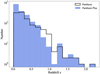 |
Fig. 1 Redshift distribution of the Pantheon and Pantheon+ samples. |
2 Pantheon+ sample
Pantheon+, as the latest sample of SNe Ia, consists of 1701 SNe Ia light curves observed from 1550 distinct SNe and covers redshift range from 0.001 to 2.26 (Brout et al. 2022; Scolnic et al. 2022). The redshift distributions of the Pantheon (Scolnic et al. 2018) and Pantheon+ samples are shown in Fig. 1. From the redshift distribution of these two samples, it is not difficult to find that there are two main differences between the new sample and the Pantheon sample. One is that the SN number has increased significantly at low redshift. There are more than 700 additional SNe in the range of z < 0.8, of which more than 500 SNe originated from z < 0.08. This is mainly because the new sample adds five large samples, including the Foundation Supernova Survey (Foundation; Foley et al. 2018), the Swift Optical/Ultraviolet Supernova Archive (SOUSA; Brown et al. 2014), the Lick Observatory Supernova Search (LOSS1; Ganeshalingam et al. 2010), the second sample from LOSS (LOSS2; Stahl et al. 2019), and the Dark Energy Survey Year 3 PES; Brout et al. 2019; Smith et al. 2020), all of which are low-redshift surveys, except DES. The other difference is that there is a significant deletion in Pantheon+ statistics between 0.8 < z < 1.0. The reason is that Scolnic et al. (2022) did not use SNe from the Supernova Legacy Survey (SNLS) at z > 0.8 considering sensitivity to the U band in model training (56 SNe in total).
Figure 2 shows the distribution (left panel) and corresponding density (right panel) of the Pantheon+ sample in the sky of the galactic coordinate system. Some previous work has pointed out that the Pantheon SNe la are not uniformly distributed in the sky; half of them are located in the galactic southeast. Some SNe are very concentrated, forming a belt-like structure that is the SDSS sample (Zhao et al. 2019). At the same time, Zhao et al. (2019) also investigated the effect of the inhomogeneous distribution of the Pantheon sample on the cosmic anisotropy and found that the belt-like structure plays the most important role in the Pantheon sample. In the left panel, to highlight the difference between these two samples, we mark the newly added SNe Ia in red. From the distribution of the Pantheon+ sample, we find that the distribution of the new data is still uneven across the sky. There are only fewer observations near (1, b) ~ (300°, −30°). Its incomplete sky coverage is primarily due to the fact that the Pantheon+ sample consists of different subsamples, following multiple measurement strategies. In order to make it easier to comprehend this focus, we also plot the density distribution of the Pantheon+ sample utilizing the plt.contour() function1, as shown in the right panel of Fig. 2. Color-coded values represent sample fraction per unit area. From the density distribution, we can more intuitively feel the inhomogeneity of sample distribution. As can be seen, the belt-like part of the Pantheon+ sample still plays the most important role, as in the case of the Pantheon sample, while the maximum density value changes from 0.24 to 0.21 (Hu et al. 2020). This means that the Pantheon+ sample is more uniform than the Pantheon sample. The newly added SNe Ia effectively weaken the dominance of the belt structure in the distribution. The Pantheon+ sample that is relatively uniform and rich in low redshift is very suitable for analyzing the local property of the Universe (Andrade et al. 2018; Luongo et al. 2022; Kalbouneh et al. 2023). Here, we used the RF method combined with the Pantheon+ sample to describe the all-sky distribution of cosmological parameters to study the local structure of the Universe, and the detailed analysis process is shown in the next section.
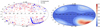 |
Fig. 2 Distribution and corresponding density contour in the galactic coordinate system. Left panel shows the SNe distribution of the Pantheon sample. Red and blue points represent the new added SNe and the SNe where the Pantheon sample and the Pan sample overlap, respectively. Right panel shows the corresponding density contour. |
3 Region fitting method
The hemisphere comparison (HC) method proposed by Schwarz & Weinhorst (2007) has been widely used in the investigation of the cosmic anisotropy, such as the anisotropy of cosmic expansion (Deng & Wei 2018a; Zhao & Xia 2022), the acceleration scale of modified Newtonian dynamics (Zhou et al. 2017; Chang et al. 2018; Chang & Zhou 2019), and the temperature anisotropy of the CMB (Hansen et al. 2004; Bennett et al. 2013; Ghosh et al. 2016; Ferreira & Quartin 2021). The RF method we used is similar to it. Here, we provide a detailed introduction to this method. Its goal is to map the all-sky distribution of the cosmological parameters. The most important step is to generate random directions  (l, b) to pick out SNe data located in specific regions to construct subdatasets, where l ∊ (0°, 360°) and b ∊ (−90°, 90°) are the longitude and latitude in the galactic coordinate system, respectively. The specific region is given by condition (θ < θmax). θ is the angle between the random direction
  (l, b) and the SN position. Here we refer to θmax as the screening angle used to obtain regions of different sizes, and the value range is (0°, 180°). The remaining steps can be divided into three parts, which we present in the following subsections.
3.1 Fitting parameters
According to subdatasets obtained in the previous step, the corresponding best fits of the cosmological parameters are obtained by minimizing value of χ2,
 (1)
(1)
where Δµ is the difference between the observational distance modulus µobs and the theoretical distance modulus µth :
 (2)
(2)
For the flat ΛCDM model, the corresponding form of µth can be written as
 (3)
(3)
here, zi is the peculiar-velocity-corrected CMB-frame redshift of each SN (Carr et al. 2022), m is the apparent magnitude of the source, M is the absolute magnitude, and dL is the luminosity distance expressed in megaparsec, defined in the following equation:
 (4)
(4)
where c is the speed of light.
The statistical (Cstat) and systematic covariance matrices (Csys) are combined and adopted to constrain the cosmological parameters:
 (5)
(5)
The datasets we used, µobs, and Cstat+sys, are provided by Brout et al. (2022) and can be obtained online2. Cstat+sys includes all the covariance between SNe (and also Cepheid host covariance) due to systematic uncertainties (Brout et al. 2022). Cstat mainly includes the full distance error and measurement noise. Csys can manifest in three key places in the analysis: (1) from changing aspects affecting the light-curve fitting; (2) from changing red-shifts that propagate to changes in distance modului relative to a cosmological model; and (3) from changes in the simulations used for bias corrections (Brout et al. 2022). More detailed information about the covariance matrices can be found in Sect. 2.2 of Brout et al. (2022). Unlike the previous analyses (Betoule et al. 2014; Colin et al. 2019), we did not introduce an intrinsic scatter. So, in the fitting process, there are only two free parameters (Ωm and H0), which makes them strongly correlated. For the different subdatasets, Ωm and H0 are fitted simultaneously. The Cstat+sys we used were obtained by cropping the total covariance matrix according to the SNe Ia subsample. In this work, the minimization was performed employing a Bayesian Markov chain Monte Carlo (MCMC; Foreman-Mackey et al. 2013) method with the emcee package3. All the fittings in this paper were obtained adopting this python package. The MCMC samples were plotted utilizing the getdist package (Lewis 2019).
3.2 All-sky distribution
During the calculation, we repeated 5000 random directions  (l, b), that is, 5000 sets of best fitting results (Ωm and H0). Based on the fitting results, the all-sky distributions of Ωm and H0 are mapped, respectively. From the distribution of Ωm and H0, we can obtain information concerning the local matter underdensity and cosmic anisotropy, respectively. In order to describe the degree of deviation from the cosmological principle, we define a parameter Dmax(σ) whose form is as follows:
 (6)
(6)
Here, Pmin and Pmax are the minimum value and the maximum value of the best fitting results, respectively.  and
and  are the corresponding 1σ error. The local matter underdensity direction and the preferred direction of cosmic anisotropy are marked by the corresponding location of the lowest Ωm and the largest H0. The corresponding 1σ regions are plotted in terms of the values of P0, which is calculated from
 (7)
(7)
where Pfit, representing the lowest Ωm constraint or the largest H0 constraint, is used to find the 1σ range of the local matter underdensity direction or the preferred direction.  represents the corresponding error. P0 represents the constraints that are consistent with Pfit within 1σ error, and
  are the corresponding 1σ values. We note that P0 and
  are filtered from the total Ωm/H0 fitting results depending on Eq. (7). Here, P0 and Pfit are completely independent and were obtained using different SNe subsamples.
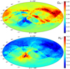 |
Fig. 3 All-sky distribution of cosmological parameters utilizing the Pantheon+ sample combined with the 90° RF method. The upper and the lower panels show the results of Ωm and H0, respectively. The corresponding values of Dmax(σ) are 3.29σ and 4.48σ, respectively. The star marks the directions of the lowest Ωm (upper panel) and the largest H0 (lower panel), and the red circle outlines the corresponding 1σ areas. The directions and 1σ areas are parameterized as Ωm,min |


3.3 Statistical analyses
In order to examine whether the discrepancy degree of the cosmological parameters from the Pantheon+ sample is consistent with statistical isotropy, we plan to carry out statistical isotropic analyses. To achieve this, we spread the original data set evenly across the sky. After that, we were able to obtain the Dmax for the isotropic dataset. Meanwhile, an additional isotropic analysis was also considered. We preserved the spatial inhomogeneity of real sample and then randomly distributed the real dataset, which randomly redistributed the distance moduli and redshift combination to real-data positions (RP) only. Given the limitations of computing time, we repeated it 500 times; this gave acceptable statistics. For convenience, we refer to these two approaches as isotropy analysis and isotropy RP analysis.
4 Results
We first give the best fitting results in the flat ΛCDM model employing the full Pantheon+ sample, Ωm = 0.36 ± 0.02, and H0 = 72.83 ± 0.23 km s−1 Mpc−1. The results are in line with the previous research (Brout et al. 2022), except that the 1σ error of H0 is reduced. The main reason is that we utilized the standardized distance modulus (µobs; Tripp 1998), where fiducial M has been determined from SH0ES 2021 Cepheid host distances (Riess et al. 2022).
After that, using the RF method with a screening angle θmax = 90°, we mapped the all-sky distribution of Ωm and H0 and draw the 1σ regions of local matter underdensity and cosmic anisotropy, as shown in the upper panel and lower panel of Fig. 3, respectively. In Fig. 3, the range of Ωm and H0 are (0.29, 0.41) and (72.03, 74.26), respectively. The corresponding differences are ΔΩm = 0.12 and ΔH0 = 2.23 km s−1 Mpc−1. The values of Dmax to Ωm and H0 are  and
and  , respectively. In the upper panel of Fig. 3, the minimum constraint of Ωm is
  (1σ) and the corresponding constraint for H0 is
  km s−1 Mpc−1. The direction and corresponding 1σ range that can be adopted to describe the local matter underdensity are
 (8)
(8)
The lower panel of Fig. 3 shows the corresponding all-sky distribution of the Hubble expansion. The maximum constraint of H0 is H0,max = 74.26 ± 0.39 km s−1 Mpc−1, and the corresponding constraint of Ωm is  . Its confidence contours are shown in Fig. 4, marked with blue lines. The preferred direction of cosmic anisotropy and corresponding 1σ range are
 (9)
(9)
In Fig. 4, we also give the best fitting results of opposite directions; that is,  km s−1 Mpc−1 and
  , which are marked with red lines.
The statistical isotropic results shown in Fig. 5 can be well described by Gaussian functions. For the isotropy analysis, the statistical significances (α) of the real data are 2.78σ for Ωm anisotropy (upper, purple panel) and 3.96σ for H0 anisotropy (upper, blue panel). The statistical significance (β) of the real data given by the isotropy RP analysis are 2.34σ for Ωm anisotropy (lower, purple panel) and 3.15σ for H0 anisotropy (lower, blue panel).
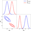 |
Fig. 4 Confidence contours (1σ and 2σ) and marginalized likelihood distributions for the parameter space (Ωm and H0) in the spatially flat ΛCDM model from the SNe Ia subsamples, which corresponds to H0,min (red line) and H0,max (blue line). The best fitting results of preferred direction are |


4.1 Reanalyses at low redshift
Recently, Hu & Wang (2022b) reported a late-time transition of H0; that is, H0 changes from a low value to a high one from early to late cosmic time by combining the GP method and H(z) data. The H0 transition occurs at z ~ 0.49. From other observations, a similar descending behavior of H0 has been found adopting other methods (see Hu & Wang 2023 for a review of H0 descending trend). Around z ~ 0.40, H0 starts to decrease (Jia et al. 2023). Both the transition behavior and the descending trend of H0 can effectively alleviate the Hubble tension. Kelly et al. (2023) gave new H0 measurements from the gravitationally lensed SNe Ia Refsdal (Refsdal 1964). The redshifts of the lens and the source are 0.54 and 1.49 (Kelly et al. 2015), respectively. Utilizing eight cluster lens models, they inferred  km s−1 Mpc−1. Then, using the two models most consistent with observations, they found
  km s−1 Mpc−1. Marking the values of lensing redshift and H0 on Fig. 3 in Hu & Wang (2022b) and Fig. 4 in Jia et al. (2023), we find that these results are in good agreement with the evolutionary behaviors of H0. Motivated by the H0 special behaviors in the late-time universe, we plan to construct a low-redshift subsample based on the Pantheon+ sample to make a reanalyses. According to the previous research (Hu & Wang 2022b; Jia et al. 2023), and considering the need for a sufficient sample size, we decided to select 1218 SNe with redshift less than 0.30 in the Pantheon+ sample to construct sub-sample (named the lp+ sample). Detailed steps and results are as follows.
At first, we give the cosmological constraint in the flat ΛCDM model using the lp+ sample; that is, Ωm = 0.44 ± 0.04 and H0 = 72.43 ± 0.30 km s−1 Mpc−1, which is consistent with the results from the full Pantheon+ sample and from Fig. 16 in Brout et al. (2022). For ease of comparison, we give the constraint results of the Pantheon+ and lp+ samples in Fig. 6. Then, we reproduced the previous analyses. The all-sky distribution, the cosmological constraints, and the isotropic statistic results are shown in Figs. 7, 8, and 9, respectively. From Fig. 7, it is easy to obtain the ranges of constraints: Ωm (0.25, 0.58) and H0 (71.43, 74.11) km s−1 Mpc−1. The corresponding differences are ∆Ωm = 0.33 and ∆H0 = 2.68 km s−1 Mpc−1. By calculation, we obtain  and
and  . The directions and 1σ regions of the local matter underdensity and cosmic anisotropy given by the reanalyses using the 1p+ sample are
 (10)
(10)
and
 (11)
(11)
The constraints corresponding to preferred directions of the local matter underdensity and cosmic anisotropy are Ωm,min = 0.25 ± 0.05 and H0 = 73.76 ± 0.41 km s−1 Mpc−1, and  km s−1 Mpc−1 and Ωm = 0.27 ± 0.06. In Fig. 8, we show the confidence contours in the preferred and opposite directions of the local matter underdensity. The isotropic statistical results from the lp+ sample are shown in Fig. 9. For the isotropy analysis, the statistical significance of the real data are 3.68σ for Ωm anisotropy (upper, purple panel) and 3.01σ for H0 anisotropy (upper, blue panel). The isotropy RP analysis gives the statistical significance of the real data, which is 2.09σ for Ωm anisotropy (lower, purple panel) and 1.35σ for H0 anisotropy (lower, blue panel).
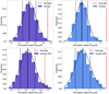 |
Fig. 5 Distribution of discrepancy degree Dmax in 500 simulated isotropic datasets. The upper two panels show the results of statistical isotropic analyses (isotropy). The lower two panels show the results of statistical isotropic analyses that preserve the spatial inhomogeneity of real data (isotropy RP). Purple and blue represent the statistical results of Ωm and H0. The black curve is the best fit to the Gaussian function. The solid black and vertical dashed lines are commensurate with the mean and the standard deviation, respectively. The red lines represent the discrepancy degree from the real data. For the isotropy analyses, the statistical significance of the real data are 2.78σ for Ωm anisotropy and 3.96σ for H0 anisotropy. For the isotropy RP analyses, the statistical significance of the real data are 2.34σ and 3.15σ for Ωm and H0 anisotropy, respectively. |
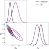 |
Fig. 6 Confidence contours (1σ and 2σ) and marginalized likelihood distributions for parameters space (Ωm and H0) in the spatially flat ACDM model from the Pantheon+ sample and the lp+ sample. For the former, the best fits are Ωm = 0.36 ± 0.02 and H0 = 72.83 ± 0.23 km s−1 Mpc−1 (black line). For the latter, the best fits are Ωm = 0.44 ± 0.04 and H0 = 72.43 ± 0.30 km s−1 Mpc−1 (purple line). |
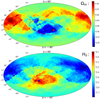 |
Fig. 7 All-sky distribution of cosmological parameters utilizing the z < 0.30 part of Pantheon+ sample (lp+ sample) combined with the 90° RF method. The upper and the lower panels show the results of Ωm and H0, respectively. The corresponding values of Dmax(σ) are 4.17σ and 4.49σ respectively. The star marks the directions of the lowest Ωm (upper panel) and the largest H0 (lower panel), and the red circle outlines the corresponding 1σ areas. The directions and 1σ areas are parameterized as |

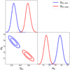 |
Fig. 8 Confidence contours (1σ and 2σ) and marginalized likelihood distributions for the parameters space (Ωm and H0) in the spatially flat ΛCDM model from the SNe Ia subsamples, which corresponds to Ωm,min (blue line) and Ωm,max (red line). The best fitting results of preferred direction are |


4.2 Different screening angles θmax
Theoretically, if there are enough SNe data distributed at different redshifts in a certain direction, the constraints of the cosmological parameters in this direction can be obtained (Lin et al. 2016a; Deng & Wei 2018b; Kumar Aluri et al. 2023). Due to the limitation of the number of observational data, it is currently impossible to directly give the result of the limitation of cosmological parameters in a certain direction. Therefore, the 90° RF method is usually used to derive the cosmological constraint of the single direction, that is the HC method (Schwarz & Weinhorst 2007). In this subsection, we try to find out the limit value of θmax that is suitable for the Pantheon+ sample by mapping the all-sky distributions of the cosmological parameters Ωm and H0 with different θmax. Considering the limitations of computing time, only three angles (30°, 45° and 60°) are chosen. Take D (60°, 0°) as an example, Fig. 10 shows the schematic diagram of the RF method with different θmax. Smaller θmax will reduce the overlapping data between sub-samples generated by adjacent random directions. The corresponding all-sky distributions will present more details on the current state of the Universe. For the Pantheon+ sample, lowering θmax can be expected to produce some poorly fitting results. Therefore, we give a constrained culling of possibly poor constraints. Here, we set a loose condition of 0 < Ωm < 1.00. The final results are shown in Fig. A.1. For the screening angles 30°, 45°, and 60°, the proportions of the wrong fitting results are 30.34%, 6.47%, and 0.70%, respectively. From Fig. A.l, we find that θmax = 60° seems to be the limit that the Pantheon+ sample can bear. At this time, nearly 100% (99.30%) of the random directions  can be reliably constrained.
In Fig. A.2, we give the best fits for the hemispheres where Ωm,min and Ωm,max are located. We find that taking into account narrowing the screening angle θmax significantly increases the 1σ error of Ωm constraints. The reduced chi-square  corresponding to Ωm,min is 0.69, which is much smaller than 1.00. Therefore, we only show the analysis results of H0. The all-sky distribution, cosmological constraints and isotropic statistical results are displayed in Figs. 11, 12, and 13, respectively. As shown in Fig. 11, the preferred direction of cosmic anisotropy given by the H0 distribution is
  , and Dmax is 4.39σ. The corresponding constraints of a preferred direction are
  km s−1 Mpc−1 and
  . The statistical isotropy results show that the statistical confidences of the real data are 1.70σ for the isotropy analysis and 2.27σ for the isotropy RP analysis.
All results in this section are summarized in Table 1. Additionally, we provide the reduced chi-square  for the anisotropic direction.
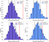 |
Fig. 9 Distribution of discrepancy degree in 500 simulated isotropic datasets. The upper two panels show the results of statistical isotropic analyses (isotropy). The lower two panels show the results of statistical isotropic analyses that preserve the spatial inhomogeneity of real data (isotropy RP). The purple and blue represent the statistical results of Ωm and H0. The black curve is the best fit to the Gaussian function. The solid black and vertical dashed lines are commensurate with the mean and the standard deviation, respectively. The red lines represent the discrepancy degree from the real data. For the isotropy analyses, the statistical significance of the real data are 3.68σ for Ωm anisotropy and 3.01σ for H0 anisotropy. For the isotropy RP analyses, the statistical significance of the real data are 2.09σ and 1.35σ for Ωm and H0 anisotropy, respectively. |
 |
Fig. 10 Schematic diagram of the RF method with different screening angles including 30°, 45°, 60°, and 90°. Black star represents the random direction |

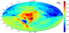 |
Fig. 11 All-sky distribution of H0 utilizing Pantheon+ sample combined with 60° RF method. The direction and 1σ area are parameterized as |

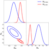 |
Fig. 12 Confidence contours (1σ and 2σ) and marginalized likelihood distributions for parameter space (Ωm and H0) in the spatially flat ΛCDM model from the SNe Ia subsamples, which corresponds to H0,min (red line) and H0,max (blue line). The best fitting results of preferred direction are |


Detailed information of analysis results from the all-sky distribution of cosmological parameters.
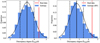 |
Fig. 13 Distribution of discrepancy degree Dmax obtained from H0 distribution in 500 simulated isotropic datasets. The left panel and right panel show the results of isotropy and isotropy RP analyses, respectively. The black curve is the best fit to the Gaussian function. The solid black and vertical dashed lines are commensurate with the mean and the standard deviation, respectively. The red lines represent the discrepancy degree from the real data. The statistical significances of the real data are 1.70σ for the isotropy analysis and 2.27σ for the isotropy RP analysis. |
5 Discussion
All-sky distributions of cosmological parameters (Ωm and H0) from the total sample show that there is an obvious local under-density area and a preferred direction of cosmic expansion. From Fig. 3, we can find that there are some weird features that may result from fluctuations in the matter density, or fluctuations in the Hubble expansion (Gurzadyan et al. 2023). In the upper panel, the red and blue areas represent areas of higher and lower material density, respectively. In the lower panel, the red areas represent regions of higher Hubble expansion. The continuity of these structures suggests that the results may not be sensitive to individual SNe Ia. Combining these two panels of Fig. 3, we find that the local underdensity in the upper panel overlaps with the higher Hubble expansion (cosmic anisotropy) in the lower panel. This may imply that local matter density might be responsible for the anisotropy of the accelerated expansion of the Universe. The corresponding 1σ regions are quite obvious. In other words, the 1σ range of Ωm is significantly larger than that of H0. The main reason for this phenomenon might be that these two parameters have different sensitivities on the redshift. The inhomogeneous matter-density distribution could also affect the decelaration parameter q0, causing a larger q0 in the local underdensity. Theoretically, the maximum q0 direction should be consistent with the local underdensity direction. For the determination of H0 value with local distance indicators, the observed H0 values depend on the average matter density within the distance range covered (Böhringer et al. 2020). Combining the Ωm distribution, we can find that there might be a region of low matter density, which leads to a smaller average matter density which makes the H0 measurements higher. Therefore, the local underdensity can exacerbate the magnitude of the Hubble Tension (Böhringer et al. 2020; Hu & Wang 2022b, 2023; Jia et al. 2023). In other words, accounting for the local underdensity or cosmic anisotropy could alleviate the current Hubble tension.
From Fig. 5, we find that the isotropy analysis shows an obvious statistical significance, especially the study of H0, which is nearly 4σ. Afterwards, considering the spatial inhomogeneity of the real sample, we performed the isotropy RP analysis and find a slight decrease in statistical significance. This suggests that inho-mogeneous spatial distribution of a real sample can increase the deviation from isotropy. In addition, combining all the statistical results, we find the statistical significations of H0 anisotropy are more obvious than that of Ωm anisotropy. From the distributions of a single parameter, we find an obvious anisotropy. But the effect of one on the other might be canceled out, making the all-sky distribution of luminosity distances isotropic. Therefore, in order to clear up this doubt, we plotted the all-sky distribution of luminosity distances when z is set to 2.26 and give the relationships between dL and z of two anisotropic hemispheres, as shown in Figs. 14 and 15, respectively. The results of these two figures show that the all-sky distribution of luminosity distances is also anisotropic and the dL − z relationships obtained from two anisotropic hemispheres have obvious differences. The direction of larger luminosity distance is consistent with the anisotropy direction from the Pantheon+ sample. All in all, our investigations from the Pantheon+ sample display an inhomogeneous and anisotropic universe, and the statistical results show no low confidence level.
Motivated by recent research (Krishnan et al. 2020, 2021b; Dainotti et al. 2021, 2022a; Colgáin et al. 2022a,b; Hu & Wang 2022b; Jia et al. 2023; Malekjani et al. 2023) hinting that H0,𝓏 might evolve with redshift, we conducted reanalyses using the low-redshift (lp+) sample. If H0 𝓏 evolves with redshift (may be caused by the local void, and so on), then the measured H0 of low-redshift and high-redshift SNe samples are different. In that case, if the redshift distribution is not uniform across the sky, this could create biases in the anisotropy detection, especially when the full sample is used; moreover, the redshift range is wider. The value of H0 obtained from the higher redshift hemisphere is smaller than that obtained from the lower redshift hemisphere. Severely uneven redshift distribution might lead to an increase in the degree of anisotropy or a bias in the anisotropy detection. The reanalysis results are similar to those of the Pantheon+ sample and verify our previous findings. From the results of the lp+ sample (Fig. 7), we find that directions of the local matter underdensity and cosmic anisotropy given by the lp+ sample are inconsistent. Comparing the results in Figs. 4 and 8, we can find that the best fits of the two anisotropic hemispheres obtained from the lp+ sample are significantly worse than the results of the total sample. In Fig. 16, we also show the relationship between Dmax and Ɀmax, the detailed information are display in Table 2. From Fig. 16, we can find that Dmax changes with Ɀmax, and has a maximum value near Ɀmax = 0.30. This might imply that the structure of the Universe changes with redshift. In addition, we also find that the influence of redshift on the all-sky distribution of Ωm is larger than that of H0. Finally, from the statistical results of lp+ sample, we also find that the statistical significance obtained from the isotropy RP analysis are lower than that from the isotropy analysis. This finding confirms that inhomogeneous spatial distribution of a real sample can increase the deviation from isotropy.
Theoretically, the screening angle θmax in the RF method can be any value between 0° and 180°. However, due to the limitations of real data in quantity, spatial part, and redshift distribution, θmax cannot be selected arbitrarily. In Sect. 4.2, we combine the RF method with the latest Pantheon+ sample, hoping to find a suitable screening angle θmax. The analysis results are shown in Fig. A.1. Finally, we find that the screening angle θmax of the Pantheon+ sample is 60°. Then, based on the 60° RF method, we restudied the Pantheon+ sample. The corresponding results are shown in Figs. 11–13. From Fig. 11, we find that there is a small area (314.16°, −22.92°) with a lower H0 value in the higher H0 area, but this structure does not appear in the RF (90°) results. The lower H0 area may be caused by high material density structures (e.g. dark matter halo) or statistical uncertainty. Narrowing the screening angle reduces the number of SNe constraining cosmological parameters, which may increase the uncertainty of the constraint. We performed a bootstrap resampling of the sample (ignoring the direction, repeated 2000 times) to study the dependence of the best-fit result error and Dmax on the number of SNe Ia used. Here, the number of SNe ranges from 100 to 700, with a total of seven groups. From the results of Fig. 17, we can find that the average error and Dmax increases as the used number of SNe decreases. The number of SNe used significantly affects the average error but does not significantly affect the Dmax value. The Dmax difference caused by the reduction in number is much smaller than the total Dmax. The preferred direction of cosmic anisotropy using the RF method with θmax = 60° is in line with that using θmax = 90° within a 1σ error. However, narrowing the screening angle means that the statistical significance of the isotropy analyses are significantly reduced. Interestingly, unlike previous findings, the statistical significance of the isotropy RP analysis is actually higher than that of the isotropy one.
Overall, we find that the all-sky distributions of cosmological parameters deviate significantly from isotropy, as shown in Figs. 3, 7, and 11. All preferred directions we obtained are consistent with each other within a 1σ range, and they are in line with previous research that traced the anisotropy of Ωm and H0 (Antoniou & Perivolaropoulos 2010; Cai & Tuo 2012; Kalus et al. 2013; Chang & Lin 2015; Hu et al. 2020) and other dipole researches (Wang & Wang 2014; Yang et al. 2014; Lin et al. 2016b; Pandey 2017; Chang & Zhou 2019; Dam et al. 2023). However, they are different from those of Luongo et al. (2022) and McConville & Colgáin (2023), which are consistent with the results of the CMB dipole (Planck Collaboration I 2016, 2020). In addition, comparing with other independent observations (as shown in Table 3) including the CMB dipole (Planck Collaboration I 2016; Planck Collaboration I 2020), dark flow (Abdalla et al. 2022), bulk flow (Turnbull et al. 2012; Feix et al. 2017; Watkins et al. 2023), and galaxy cluster (Migkas et al. 2021), it is easy to find that the directions of the larger H0 and the smaller Ωm are not consistent with the CMB dipole (Planck Collaboration I 2016; Planck Collaboration I 2020), but they coincide with the bulk flow (Turnbull et al. 2012; Feix et al. 2017; Watkins et al. 2023) and the galaxy cluster (Migkas et al. 2021). To facilitate understanding, we aggregated these results with the ones we obtained, marking them on the galactic coordinate system, as shown in Fig. 18. The effect of peculiar velocities and the bulk flow on SNe Ia cosmology has already been discussed (Hui & Greene 2006; Davis et al. 2011; Betoule et al. 2014; Rameez et al. 2018). They can make a tiny shift in the best-fit cosmological parameters and the preferred direction locally (Colin et al. 2019).
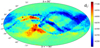 |
Fig. 14 All-sky distribution of luminosity distance dL utilizing the Pantheon+ sample combined with the 90° RF method. Here, we fix 𝓏 = 2.26. |
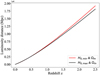 |
Fig. 15 Relationships between dL and 𝓏 of two anisotropic hemispheres using the two sets of best fits (H0,min, Ωm and H0,max, Ωm) in the H0 distribution. |
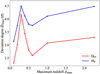 |
Fig. 16 Relationship between discrepancy degree Dmax and Ɀmax· |
Detailed information on the investigation of the relationship between the discrepancy degree Dmax and Ɀmax.
Preferred directions given by other independent observations.
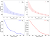 |
Fig. 17 Relationship between average error and discrepancy degree Dmax and SN number used. The upper panels show the relationship between the average error and the used SN number. The lower panels show the relationship between the discrepancy degree Dmax and the SN number used. Blue and red correspond to parameters Ωm and H0, respectively. |
6 Conclusions and perspectives
In this paper, we propose the RF method for the first time and combine this method with the Pantheon+ sample to test the cos-mological principle. From the matter density and the Hubble expansion distributions mapped using the RF method, we find that the all-sky distributions of cosmological parameters deviate significantly from isotropy. The corresponding distribution of luminosity distance also deviates from isotropy; that is, the dL-z relation actually diverges from region to region. Results of statistical isotropy analyses (isotropy and isotropy RP) show relatively high confidence levels: 2.78σ (isotropy) and 2.34σ (isotropy RP) for the local matter underdensity, 3.96σ (isotropy) and 3.15σ (isotropy RP) for the cosmic anisotropy. Comparing the results of statistical isotropy analyses, we find that inhomogeneous spatial distribution of real sample can increase the deviation from isotropy. The statistical significations of H0 anisotropy are more obvious than that of Ωm anisotropy. This might hint that parameter H0 is more sensitive to cosmic anisotropy. The similar results and findings are found from reanalyses of the lp+ sample and the lower screening angle (θmax = 60°), but with a slight decrease in statistical significance. In addition, we find that Dmax changes with zmax and has a maximum value near zmax = 0.30. The average error and Dmax increase as the used number of SNe decreases. Comparing with the previous researches, we find all preferred directions we obtained are in line with that were provided by Antoniou & Perivolaropoulos (2010), Cai & Tuo (2012), Wang & Wang (2014), Yang et al. (2014), Kalus et al. (2013), Chang & Lin (2015), Lin et al. (2016b), Chang & Zhou (2019), and Hu et al. (2020), but they are not consistent with those given by Luongo et al. (2022) and McConville & Colgáin (2023).
Until now, many SNe Ia have been observed and have been widely used for cosmological applications (Hoscheit & Barger 2018; Perivolaropoulos & Skara 2021; Cowell et al. 2023; Hu & Wang 2022a; Wang et al. 2022; Briffa et al. 2023)4. However, there is still an inhomogeneous distribution in data, which significantly affects the testing of cosmological principle. One way to solve this problem is to add some new SNe Ia measurements, and another way is to consider other independent observations; for example, quasar (Lusso & Risaliti 2016, 2017; Bisogni et al. 2017; Risaliti & Lusso 2019; Cao et al. 2022b; Khadka et al. 2022; Liu et al. 2023a; Zajaček et al. 2023), gamma-ray burst (GRB; Wang et al. 2015, 2022; Shirokov et al. 2020; Hu et al. 2021; Cao et al. 2022a; Liu et al. 2022b; Lovyagin et al. 2022; Liang et al. 2022), fast radio burst (FRB; Hagstotz et al. 2022; Wu et al. 2022; James et al. 2022; Zhao et al. 2022; Gao et al. 2024; Liu et al. 2023b), Tip of the Red Giant Branch (TRGB; Freedman et al. 2019, 2020; Freedman 2021), galaxy cluster (Javanmardi & Kroupa 2017; Migkas et al. 2020, 2021), and gravitational wave (GW; Abbott et al. 2017; Chen et al. 2018; Jin et al. 2023; Wang et al. 2023b) observations, among others. At present, these observations may still have some deficiencies in quantity or quality, but this situation is expected to improve in the future. The e-ROSITA all-sky survey (Merloni et al. 2012; Predehl 2012; Kolodzig et al. 2013; Lusso 2020), Einstein Probe (EP; Yuan et al. 2015), French-Chinese satellite space-based multi-band astronomical variable objects monitor (SVOM; Wei et al. 2016), China Space Station Telescope (CSST) photometric survey (Xu et al. 2022; Miao et al. 2023; Li et al. 2023a), and Transient High-Energy Sky and Early Universe Surveyor (THESEUS; Amati et al. 2018) space missions together with ground- and space-based multi-messenger facilities will provide a lot of observations and measurements, improve the observational quality, and probe the poorly explored high-redshift universe. The Australian Square Kilometer Array Pathfinder (ASKAP; Chapman et al. 2017), MeerKAT (Sanidas et al. 2018), Very Large Array (VLA; Law et al. 2018), and Canadian Hydrogen Intensity Mapping Experiment (CHIME)/FRB Outriggers (Leung et al. 2021) will provide a large number of positioned FRBs in the future, which will give higher precision cosmological constraints. In addition, the Advanced Laser Interferometer Gravitational-wave Observatory (aLIGO; LIGO Scientific Collaboration 2015) and Virgo (Acernese et al. 2015) detectors will provide more GW events. In combination with the electromagnetic counterparts, model-independent constraints will be given on the cosmological parameters. The high-quality observations enable us to examine the cosmological principle at higher redshifts and investigate whether the Hubble tension is related to the failure of the cosmological principle.
Notes: As this work was about to be completed, Perivolaropoulos (2023) used the HC method to test the cosmic isotropy of the SNe Ia absolute magnitudes from the Pantheon+ and SH0ES samples in various redshift/distance bins. They found that sharp changes of the level of anisotropy occuring at distances under 40 Mpc in the real samples. If there are enough local observations in the future, more local information about our Universe could be obtained by combining our method with the idea of Perivolaropoulos (2023). This will be pursued in future work.
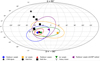 |
Fig. 18 Distribution of preferred directions (l, b) with 1σ range in other independent observations. We mark the directions given by Ωm with plus signs at different screening angles, and the directions given by H0 are shown with triangles at different screening angles. The color represents the important result obtained in this work; black shows the result given by other independent observations including the CMB dipole (Planck Collaboration I 2016; Planck Collaboration I 2020), dark flow (Abdalla et al. 2022), bulk flow (Turnbull et al. 2012; Feix et al. 2017; Watkins et al. 2023), and galaxy cluster (Migkas et al. 2021). |
Acknowledgements
We thank the anonymous referee for constructive comments. This work was supported by the National Natural Science Foundation of China (grant No. 12273009), the China Manned Spaced Project (CMS-CSST-2021-A12), Jiangsu Funding Program for Excellent Postdoctoral Talent (20220ZB59), Project funded by China Postdoctoral Science Foundation (2022M72l56l), NWO, the Dutch Research Council, under Vici research programme 'ARGO' with project number 639.043.815, Yunnan Youth Basic Research Projects 202001AU070013 and National Natural Science Foundation of China (grant no. 12303050).
Appendix A Additional figures
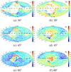 |
Fig. A.1 All-sky distribution of cosmological parameter (Ωm and H0) utilizing the Pantheon+ sample combined with the RF method with different screening angles including 30°, 45°, and 60°. Panels (a) and (b) show the results using the RF method with 30°. Panels (c) and (d) are the results of 45°. Panels (e) and (f) are the results of 60°. The proportions of the wrong fitting results are 30.34%, 6.47%, and 0.70% for the screening angles 30°, 45°, and 60°, respectively. |
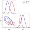 |
Fig. A.2 Confidence contours (1σ and 2σ) and marginalized likelihood distributions for parameters space (Ωm and H0) in the spatially flat ΛCDM model from SNe la subsamples, which corresponds to Ωmmin and Ωm,max. The best fits are |


References
- Abbott, B. P., Abbott, R., Abbott, T. D., et al. 2017, Nature, 551, 85 [Google Scholar]
- Abbott, T. M. C., Alarcon, A., Allam, S., et al. 2019, Phys. Rev. Lett., 122, 171301 [NASA ADS] [CrossRef] [Google Scholar]
- Abdalla, E., Abellán, G. F., Aboubrahim, A., et al. 2022, J. High Energy Astrophys., 34, 49 [NASA ADS] [CrossRef] [Google Scholar]
- Acernese, F., Agathos, M., Agatsuma, K., et al. 2015, Class. Quant. Grav., 32, 024001 [Google Scholar]
- Akarsu, Ö., Barrow, J. D., & Uzun, N. M. 2020, Phys. Rev. D, 102, 124059 [NASA ADS] [CrossRef] [Google Scholar]
- Akarsu, Ö., Dereli, T., & Katirci, N. 2022, J. Phys. Conf. Ser., 2191, 012001 [NASA ADS] [CrossRef] [Google Scholar]
- Akarsu, Ö., Di Valentino, E., Kumar, S., Özyigit, M., & Sharma, S. 2023, Phys. Dark Universe, 39, 101162 [NASA ADS] [CrossRef] [Google Scholar]
- Amati, L., O’Brien, P., Götz, D., et al. 2018, Adv. Space Res., 62, 191 [Google Scholar]
- Andrade, U., Bengaly, C. A. P., Santos, B., & Alcaniz, J. S. 2018, ApJ, 865, 119 [NASA ADS] [CrossRef] [Google Scholar]
- Antoniou, I., & Perivolaropoulos, L. 2010, J. Cosmology Astropart. Phys., 2010, 012 [NASA ADS] [CrossRef] [Google Scholar]
- Bargiacchi, G., Dainotti, M. G., Nagataki, S., & Capozziello, S. 2023, MNRAS, 521, 3909 [NASA ADS] [CrossRef] [Google Scholar]
- Bayron Orjuela-Quintana, J., Álvarez, M., Valenzuela-Toledo, C. A., & Rodríguez, Y. 2020, J. Cosmology Astropart. Phys., 2020, 019 [CrossRef] [Google Scholar]
- Bennett, C. L., Halpern, M., Hinshaw, G., et al. 2003, ApJS, 148, 1 [Google Scholar]
- Bennett, C. L., Hill, R. S., Hinshaw, G., et al. 2011, ApJS, 192, 17 [NASA ADS] [CrossRef] [Google Scholar]
- Bennett, C. L., Larson, D., Weiland, J. L., et al. 2013, ApJS, 208, 20 [Google Scholar]
- Betoule, M., Kessler, R., Guy, J., et al. 2014, A&A, 568, A22 [NASA ADS] [CrossRef] [EDP Sciences] [Google Scholar]
- Bielewicz, P., Górski, K. M., & Banday, A. J. 2004, MNRAS, 355, 1283 [NASA ADS] [CrossRef] [Google Scholar]
- Bisogni, S., Risaliti, G., & Lusso, E. 2017, Front. Astron. Space Sci., 4, 68 [Google Scholar]
- Böhringer, H., Chon, G., & Collins, C. A. 2020, A&A, 633, A19 [EDP Sciences] [Google Scholar]
- Bonvin, C., Durrer, R., & Kunz, M. 2006, Phys. Rev. Lett., 96, 191302 [NASA ADS] [CrossRef] [Google Scholar]
- Briffa, R., Escamilla-Rivera, C., Said, J. L., & Mifsud, J. 2023, MNRAS, 522, 6024 [CrossRef] [Google Scholar]
- Brout, D., Sako, M., Scolnic, D., et al. 2019, ApJ, 874, 106 [NASA ADS] [CrossRef] [Google Scholar]
- Brout, D., Scolnic, D., Popovic, B., et al. 2022, ApJ, 938, 110 [NASA ADS] [CrossRef] [Google Scholar]
- Brown, P. J., Breeveld, A. A., Holland, S., Kuin, P., & Pritchard, T. 2014, Ap&SS, 354, 89 [Google Scholar]
- Cai, R.-G., & Tuo, Z.-L. 2012, J. Cosmology Astropart. Phys., 2012, 004 [NASA ADS] [CrossRef] [Google Scholar]
- Cai, R.-G., Ding, J.-F., Guo, Z.-K., Wang, S.-J., & Yu, W.-W. 2021, Phys. Rev. D, 103, 123539 [NASA ADS] [CrossRef] [Google Scholar]
- Cai, T., Ding, Q., & Wang, Y. 2022, arXiv e-prints [arXiv:2211.06857] [Google Scholar]
- Camarena, D., Marra, V., Sakr, Z., & Clarkson, C. 2022, Class. Quant. Grav., 39, 184001 [NASA ADS] [CrossRef] [Google Scholar]
- Cao, S., & Ratra, B. 2022, MNRAS, 513, 5686 [Google Scholar]
- Cao, S., & Ratra, B. 2023, Phys. Rev. D, 107, 103521 [NASA ADS] [CrossRef] [Google Scholar]
- Cao, S., Khadka, N., & Ratra, B. 2022a, MNRAS, 510, 2928 [NASA ADS] [CrossRef] [Google Scholar]
- Cao, S., Zajacek, M., Panda, S., et al. 2022b, MNRAS, 516, 1721 [NASA ADS] [CrossRef] [Google Scholar]
- Capozziello, S., Sarracino, G., & Spallicci, A. D. A. M. 2023, Phys. Dark Universe, 40, 101201 [NASA ADS] [CrossRef] [Google Scholar]
- Carr, A., Davis, T. M., Scolnic, D., et al. 2022, PASA, 39, e046 [CrossRef] [Google Scholar]
- Castello, S., Högås, M., & Mörtsell, E. 2022, J. Cosmology Astropart. Phys., 2022, 003 [CrossRef] [Google Scholar]
- Chang, Z., & Lin, H.-N. 2015, MNRAS, 446, 2952 [Google Scholar]
- Chang, Z., & Zhou, Y. 2019, MNRAS, 486, 1658 [CrossRef] [Google Scholar]
- Chang, Z., Lin, H.-N., Zhao, Z.-C., &Zhou, Y. 2018, Chinese Phys. C, 42, 115103 [NASA ADS] [CrossRef] [Google Scholar]
- Chapman, J. M., Dempsey, J., Miller, D., et al. 2017, ASP Conf. Ser., 512, 73 [Google Scholar]
- Chen, H.-Y. 2019, Nat. Astron., 3, 384 [CrossRef] [Google Scholar]
- Chen, H.-Y., Fishbach, M., & Holz, D. E. 2018, Nature, 562, 545 [Google Scholar]
- Colgáin, E. Ó., Sheikh-Jabbari, M. M., Solomon, R., Dainotti, M. G., & Stojkovic, D. 2022a, arXiv e-prints [arXiv:2206.11447] [Google Scholar]
- Colgáin, E. Ó., Sheikh-Jabbari, M. M., Solomon, R., et al. 2022b, Phys. Rev. D, 106, L041301 [CrossRef] [Google Scholar]
- Colgáin, E. Ó., Sheikh-Jabbari, M. M., & Solomon, R. 2023, Phys. Dark Universe, 40, 101216 [CrossRef] [Google Scholar]
- Colin, J., Mohayaee, R., Sarkar, S., & Shafieloo, A. 2011, MNRAS, 414, 264 [Google Scholar]
- Colin, J., Mohayaee, R., Rameez, M., & Sarkar, S. 2017, MNRAS, 471, 1045 [Google Scholar]
- Colin, J., Mohayaee, R., Rameez, M., & Sarkar, S. 2019, A&A, 631, L13 [NASA ADS] [CrossRef] [EDP Sciences] [Google Scholar]
- Cowell, J. A., Dhawan, S., & Macpherson, H. J. 2023, MNRAS, 526, 1482 [NASA ADS] [CrossRef] [Google Scholar]
- Dainotti, M. G., De Simone, B., Schiavone, T., et al. 2021, ApJ, 912, 150 [NASA ADS] [CrossRef] [Google Scholar]
- Dainotti, M. G., De Simone, B. D., Schiavone, T., et al. 2022a, Galaxies, 10, 24 [NASA ADS] [CrossRef] [Google Scholar]
- Dainotti, M. G., Nielson, V., Sarracino, G., et al. 2022b, MNRAS, 514, 1828 [CrossRef] [Google Scholar]
- Dam, L., Lewis, G. F., & Brewer, B. J. 2023, MNRAS, 525, 231 [NASA ADS] [CrossRef] [Google Scholar]
- Davis, T. M., Hui, L., Frieman, J. A., et al. 2011, ApJ, 741, 67 [NASA ADS] [CrossRef] [Google Scholar]
- de Cruz Pérez, J., Park, C.-G., & Ratra, B. 2023, Phys. Rev. D, 107, 063522 [CrossRef] [Google Scholar]
- de Jaeger, T., & Galbany, L. 2023, arXiv e-prints [arXiv:2305.17243] [Google Scholar]
- Deng, H.-K., & Wei, H. 2018a, Eur. Phys. J. C, 78, 755 [NASA ADS] [CrossRef] [Google Scholar]
- Deng, H.-K., & Wei, H. 2018b, Phys. Rev. D, 97, 123515 [NASA ADS] [CrossRef] [Google Scholar]
- Dhawan, S., Borderies, A., Macpherson, H. J., & Heinesen, A. 2023, MNRAS, 519, 4841 [NASA ADS] [CrossRef] [Google Scholar]
- Di Valentino, E., Mena, O., Pan, S., et al. 2021, Class. Quant. Grav., 38, 153001 [NASA ADS] [CrossRef] [Google Scholar]
- Ebrahimian, E., Krishnan, C., Mondol, R., & Sheikh-Jabbari, M. M. 2023, arXiv e-prints [arXiv:2305.16177] [Google Scholar]
- Enqvist, K. 2008, General Relativity Gravitation, 40, 451 [NASA ADS] [CrossRef] [Google Scholar]
- Feix, M., Branchini, E., & Nusser, A. 2017, MNRAS, 468, 1420 [NASA ADS] [CrossRef] [Google Scholar]
- Ferreira, P. d. S., & Quartin, M. 2021, Phys. Rev. D, 104, 063503 [NASA ADS] [CrossRef] [Google Scholar]
- Foley, R. J., Scolnic, D., Rest, A., et al. 2018, MNRAS, 475, 193 [Google Scholar]
- Foreman-Mackey, D., Hogg, D. W., Lang, D., & Goodman, J. 2013, PASP, 125, 306 [Google Scholar]
- Freedman, W. L. 2021, ApJ, 919, 16 [NASA ADS] [CrossRef] [Google Scholar]
- Freedman, W. L., Madore, B. F., Hatt, D., et al. 2019, ApJ, 882, 34 [Google Scholar]
- Freedman, W. L., Madore, B. F., Hoyt, T., et al. 2020, ApJ, 891, 57 [Google Scholar]
- Ganeshalingam, M., Li, W., Filippenko, A. V., et al. 2010, ApJS, 190, 418 [NASA ADS] [CrossRef] [Google Scholar]
- Gao, J., Zhou, Z., Du, M., et al. 2024, MNRAS, 527, 7861 [Google Scholar]
- Garcia-Bellido, J., & Haugbølle, T. 2008, J. Cosmology Astropart. Phys., 2008, 003 [CrossRef] [Google Scholar]
- Ghosh, S., & Jain, P. 2020, MNRAS, 492, 3994 [NASA ADS] [CrossRef] [Google Scholar]
- Ghosh, S., Kothari, R., Jain, P., & Rath, P. K. 2016, J. Cosmology Astropart. Phys., 2016, 046 [CrossRef] [Google Scholar]
- Gruppuso, A., Finelli, F., Natoli, P., et al. 2011, MNRAS, 411, 1445 [CrossRef] [Google Scholar]
- Gurzadyan, V. G., Fimin, N. N., & Chechetkin, V. M. 2023, A&A, 677, A161 [NASA ADS] [CrossRef] [EDP Sciences] [Google Scholar]
- Hagstotz, S., Reischke, R., & Lilow, R. 2022, MNRAS, 511, 662 [CrossRef] [Google Scholar]
- Hamaus, N., Aubert, M., Pisani, A., et al. 2022, A&A, 658, A20 [NASA ADS] [CrossRef] [EDP Sciences] [Google Scholar]
- Hansen, F. K., Banday, A. J., & Górski, K. M. 2004, MNRAS, 354, 641 [NASA ADS] [CrossRef] [Google Scholar]
- Haslbauer, M., Banik, I., & Kroupa, P. 2020, MNRAS, 499, 2845 [Google Scholar]
- Horstmann, N., Pietschke, Y., & Schwarz, D. J. 2022, A&A, 668, A34 [NASA ADS] [CrossRef] [EDP Sciences] [Google Scholar]
- Hoscheit, B. L., & Barger, A. J. 2018, ApJ, 854, 46 [NASA ADS] [CrossRef] [Google Scholar]
- Hu, J. P., & Wang, F. Y. 2022a, A&A, 661, A71 [NASA ADS] [CrossRef] [EDP Sciences] [Google Scholar]
- Hu, J. P., & Wang, F. Y. 2022b, MNRAS, 517, 576 [NASA ADS] [CrossRef] [Google Scholar]
- Hu, J.-P., & Wang, F.-Y. 2023, Universe, 9, 94 [CrossRef] [Google Scholar]
- Hu, J. P., Wang, Y. Y., & Wang, F. Y. 2020, A&A, 643, A93 [EDP Sciences] [Google Scholar]
- Hu, J. P., Wang, F. Y., & Dai, Z. G. 2021, MNRAS, 507, 730 [NASA ADS] [CrossRef] [Google Scholar]
- Hu, J., Hu, J.-P., Li, Z., Zhao, W., & Chen, J. 2023, Phys. Rev. D, 108, 083024 [NASA ADS] [CrossRef] [Google Scholar]
- Hui, L., & Greene, P. B. 2006, Phys. Rev. D, 73, 123526 [NASA ADS] [CrossRef] [Google Scholar]
- Hutsemékers, D., Cabanac, R., Lamy, H., & Sluse, D. 2005, A&A, 441, 915 [Google Scholar]
- Hwang, H. S., Geller, M. J., Park, C., et al. 2016, ApJ, 818, 173 [NASA ADS] [CrossRef] [Google Scholar]
- James, C. W., Ghosh, E. M., Prochaska, J. X., et al. 2022, MNRAS, 516, 4862 [NASA ADS] [CrossRef] [Google Scholar]
- Javanmardi, B., & Kroupa, P. 2017, A&A, 597, A120 [NASA ADS] [CrossRef] [EDP Sciences] [Google Scholar]
- Javanmardi, B., Porciani, C., Kroupa, P., & Pflamm-Altenburg, J. 2015, ApJ, 810, 47 [NASA ADS] [CrossRef] [Google Scholar]
- Jia, X. D., Hu, J. P., Yang, J., Zhang, B. B., & Wang, F. Y. 2022, MNRAS, 516, 2575 [Google Scholar]
- Jia, X. D., Hu, J. P., & Wang, F. Y. 2023, A&A, 674, A45 [NASA ADS] [CrossRef] [EDP Sciences] [Google Scholar]
- Jin, S.-J., Xing, S.-S., Shao, Y., Zhang, J.-F., & Zhang, X. 2023, Chinese Phys. C, 47, 065104 [NASA ADS] [CrossRef] [Google Scholar]
- Kalbouneh, B., Marinoni, C., & Bel, J. 2023, Phys. Rev. D, 107, 023507 [NASA ADS] [CrossRef] [Google Scholar]
- Kalus, B., Schwarz, D. J., Seikel, M., & Wiegand, A. 2013, A&A, 553, A56 [NASA ADS] [CrossRef] [EDP Sciences] [Google Scholar]
- Kazantzidis, L., & Perivolaropoulos, L. 2020, Phys. Rev. D, 102, 023520 [Google Scholar]
- Keenan, R. C., Barger, A. J., & Cowie, L. L. 2013, ApJ, 775, 62 [NASA ADS] [CrossRef] [Google Scholar]
- Kelly, P. L., Rodney, S. A., Treu, T., et al. 2015, Science, 347, 1123 [Google Scholar]
- Kelly, P. L., Rodney, S., Treu, T., et al. 2023, Science, 380, abh1322 [NASA ADS] [CrossRef] [Google Scholar]
- Kenworthy, W. D., Scolnic, D., & Riess, A. 2019, ApJ, 875, 145 [NASA ADS] [CrossRef] [Google Scholar]
- Khadka, N., & Ratra, B. 2020, MNRAS, 492, 4456 [NASA ADS] [CrossRef] [Google Scholar]
- Khadka, N., Zajacek, M., Panda, S., Martínez-Aldama, M. L., & Ratra, B. 2022, MNRAS, 515, 3729 [NASA ADS] [CrossRef] [Google Scholar]
- Khadka, N., Zajacek, M., Prince, R., et al. 2023, MNRAS, 522, 1247 [NASA ADS] [CrossRef] [Google Scholar]
- King, J. A., Webb, J. K., Murphy, M. T., et al. 2012, MNRAS, 422, 3370 [Google Scholar]
- Koivisto, T., & Mota, D. F. 2008, J. Cosmology Astropart. Phys., 2008, 018 [CrossRef] [Google Scholar]
- Koksbang, S. M. 2021, Phys. Rev. Lett., 126, 231101 [NASA ADS] [CrossRef] [Google Scholar]
- Kolodzig, A., Gilfanov, M., Sunyaev, R., Sazonov, S., & Brusa, M. 2013, A&A, 558, A89 [NASA ADS] [CrossRef] [EDP Sciences] [Google Scholar]
- Krishnan, C., Colgáin, E. Ó., Ruchika, Sen, A. A., Sheikh-Jabbari, M. M., & Yang, T. 2020, Phys. Rev. D, 102, 103525 [NASA ADS] [CrossRef] [Google Scholar]
- Krishnan, C., Mohayaee, R., Colgáin, E. Ó., Sheikh-Jabbari, M. M., & Yin, L. 2021a, Class. Quant. Grav., 38, 184001 [NASA ADS] [CrossRef] [Google Scholar]
- Krishnan, C., Ó Colgáin, E., Sheikh-Jabbari, M. M., & Yang, T. 2021b, Phys. Rev. D, 103, 103509 [NASA ADS] [CrossRef] [Google Scholar]
- Krishnan, C., Mohayaee, R., Colgáin, E. Ó., Sheikh-Jabbari, M. M., & Yin, L. 2022, Phys. Rev. D, 105, 063514 [NASA ADS] [CrossRef] [Google Scholar]
- Kroupa, P., Gjergo, E., Asencio, E., et al. 2023, arXiv e-prints [arXiv:2309.11552] [Google Scholar]
- Kumar, D., Choudhury, D., & Nandi, D. 2023, arXiv e-prints [arXiv:2310.03509] [Google Scholar]
- Kumar Aluri, P., Cea, P., Chingangbam, P., et al. 2023, Class. Quant. Grav., 40, 094001 [NASA ADS] [CrossRef] [Google Scholar]
- Lapi, A., Boco, L., Cueli, M. M., et al. 2023, ApJ, 959, 83 [NASA ADS] [CrossRef] [Google Scholar]
- Law, C. J., Bower, G. C., Burke-Spolaor, S., et al. 2018, ApJS, 236, 8 [NASA ADS] [CrossRef] [Google Scholar]
- Leung, C., Mena-Parra, J., Masui, K., et al. 2021, AJ, 161, 81 [NASA ADS] [CrossRef] [Google Scholar]
- Lewis, A. 2019, arXiv e-prints [arXiv:1910.13970] [Google Scholar]
- Li, X., & Lin, H.-N. 2017, Chinese Phys. C, 41, 065102 [NASA ADS] [CrossRef] [Google Scholar]
- Li, S.-Y., Li, Y.-L., Zhang, T., et al. 2023a, Sci. China Phys. Mech. Astron., 66, 229511 [NASA ADS] [CrossRef] [Google Scholar]
- Li, Z., Zhang, B., & Liang, N. 2023b, MNRAS, 521, 4406 [CrossRef] [Google Scholar]
- Liang, N., Li, Z., Xie, X., & Wu, P. 2022, ApJ, 941, 84 [CrossRef] [Google Scholar]
- LIGO Scientific Collaboration (Aasi, J., et al.) 2015, Class. Quant. Grav., 32, 074001 [Google Scholar]
- Lin, H.-N., Li, X., & Chang, Z. 2016a, MNRAS, 460, 617 [NASA ADS] [CrossRef] [Google Scholar]
- Lin, H.-N., Wang, S., Chang, Z., & Li, X. 2016b, MNRAS, 456, 1881 [NASA ADS] [CrossRef] [Google Scholar]
- Liu, Y., Chen, F., Liang, N., et al. 2022a, ApJ, 931, 50 [NASA ADS] [CrossRef] [Google Scholar]
- Liu, Y., Liang, N., Xie, X., et al. 2022b, ApJ, 935, 7 [NASA ADS] [CrossRef] [Google Scholar]
- Liu, T., Yang, X., Zhang, Z., Wang, J., & Biesiada, M. 2023a, Phys. Lett. B, 845, 138166 [NASA ADS] [CrossRef] [Google Scholar]
- Liu, Y., Yu, H., & Wu, P. 2023b, ApJ, 946, L49 [NASA ADS] [CrossRef] [Google Scholar]
- Lovyagin, N. Y., Gainutdinov, R. I., Shirokov, S. I., & Gorokhov, V. L. 2022, Universe, 8, 344 [NASA ADS] [CrossRef] [Google Scholar]
- Luković, V. V., Haridasu, B. S., & Vittorio, N. 2020, MNRAS, 491, 2075 [Google Scholar]
- Luongo, O., Muccino, M., Colgáin, E. Ó., Sheikh-Jabbari, M. M., & Yin, L. 2022, Phys. Rev. D, 105, 103510 [NASA ADS] [CrossRef] [Google Scholar]
- Lusso, E. 2020, Front. Astron. Space Sci., 7, 8 [NASA ADS] [CrossRef] [Google Scholar]
- Lusso, E., & Risaliti, G. 2016, ApJ, 819, 154 [Google Scholar]
- Lusso, E., & Risaliti, G. 2017, A&A, 602, A79 [NASA ADS] [CrossRef] [EDP Sciences] [Google Scholar]
- Malekjani, M., Mc Conville, R., Colgáin, E. Ó., Pourojaghi, S., & Sheikh-Jabbari, M. M. 2023, arXiv e-prints [arXiv:2301.12725] [Google Scholar]
- Mandal, S., Duffell, P. C., Polin, A., & Milisavljevic, D. 2023, ApJ, 956, 130 [NASA ADS] [CrossRef] [Google Scholar]
- Mariano, A., & Perivolaropoulos, L. 2012, Phys. Rev. D, 86, 083517 [NASA ADS] [CrossRef] [Google Scholar]
- McConville, R., & Colgáin, E. Ó. 2023, Phys. Rev. D, 108, 123533 [CrossRef] [Google Scholar]
- Merloni, A., Predehl, P., Becker, W., et al. 2012, arXiv e-prints [arXiv:1209.3114] [Google Scholar]
- Miao, H., Gong, Y., Chen, X., et al. 2023, MNRAS, 519, 1132 [Google Scholar]
- Migkas, K., Schellenberger, G., Reiprich, T. H., et al. 2020, A&A, 636, A15 [NASA ADS] [CrossRef] [EDP Sciences] [Google Scholar]
- Migkas, K., Pacaud, F., Schellenberger, G., et al. 2021, A&A, 649, A151 [NASA ADS] [CrossRef] [EDP Sciences] [Google Scholar]
- Milaković, D., Lee, C.-C., Molaro, P., & Webb, J. K. 2022, arXiv e-prints [arXiv:2212.02458] [Google Scholar]
- Millon, M., Galan, A., Courbin, F., et al. 2020, A&A, 639, A101 [NASA ADS] [CrossRef] [EDP Sciences] [Google Scholar]
- Mohammadi, S., Yusofi, E., Mohsenzadeh, M., & Salem, M. K. 2023, MNRAS, 525, 3274 [NASA ADS] [CrossRef] [Google Scholar]
- Motoa-Manzano, J., Orjuela-Quintana, J. B., Pereira, T. S., & Valenzuela-Toledo, C. A. 2021, Phys. Dark Universe, 32, 100806 [NASA ADS] [CrossRef] [Google Scholar]
- Pandey, B. 2017, MNRAS, 468, 1953 [NASA ADS] [CrossRef] [Google Scholar]
- Pastén, E., & Cárdenas, V. H. 2023, Phys. Dark Universe, 40, 101224 [CrossRef] [Google Scholar]
- Pedregosa, F., Varoquaux, G., Gramfort, A., et al. 2011, J. Mach. Learn. Res., 12, 2825 [Google Scholar]
- Pelgrims, V., & Hutsemékers, D. 2016, A&A, 590, A53 [NASA ADS] [CrossRef] [EDP Sciences] [Google Scholar]
- Perivolaropoulos, L. 2023, Phys. Rev. D, 108, 063509 [NASA ADS] [CrossRef] [Google Scholar]
- Perivolaropoulos, L., & Skara, F. 2021, Phys. Rev. D, 104, 123511 [NASA ADS] [CrossRef] [Google Scholar]
- Perivolaropoulos, L., & Skara, F. 2022, New Astron. Rev., 95, 101659 [CrossRef] [Google Scholar]
- Perivolaropoulos, L., & Skara, F. 2023, MNRAS, 520, 5110 [NASA ADS] [CrossRef] [Google Scholar]
- Planck Collaboration I. 2016, A&A, 594, A1 [NASA ADS] [CrossRef] [EDP Sciences] [Google Scholar]
- Planck Collaboration I. 2020, A&A, 641, A1 [NASA ADS] [CrossRef] [EDP Sciences] [Google Scholar]
- Planck Collaboration VI. 2020, A&A, 641, A6 [NASA ADS] [CrossRef] [EDP Sciences] [Google Scholar]
- Planck Collaboration VII. 2020, A&A, 641, A7 [NASA ADS] [CrossRef] [EDP Sciences] [Google Scholar]
- Porredon, A., Crocce, M., Elvin-Poole, J., et al. 2022, Phys. Rev. D, 106, 103530 [NASA ADS] [CrossRef] [Google Scholar]
- Predehl, P. 2012, SPIE Conf. Ser., 8443, 84431R [Google Scholar]
- Rahman, W., Trotta, R., Boruah, S. S., Hudson, M. J., & van Dyk, D. A. 2022, MNRAS, 514, 139 [NASA ADS] [CrossRef] [Google Scholar]
- Rameez, M., Mohayaee, R., Sarkar, S., & Colin, J. 2018, MNRAS, 477, 1772 [Google Scholar]
- Refsdal, S. 1964, MNRAS, 128, 295 [NASA ADS] [CrossRef] [Google Scholar]
- Riess, A. G. 2020, Nat. Rev. Phys., 2, 10 [NASA ADS] [CrossRef] [Google Scholar]
- Riess, A. G. & Breuval, L. 2023, arXiv e-prints [arXiv: 2308.10954] [Google Scholar]
- Riess, A. G., Casertano, S., Yuan, W., Macri, L. M., & Scolnic, D. 2019, ApJ, 876, 85 [Google Scholar]
- Riess, A. G., Yuan, W., Macri, L. M., et al. 2022, ApJ, 934, L7 [NASA ADS] [CrossRef] [Google Scholar]
- Risaliti, G., & Lusso, E. 2019, Nat. Astron., 3, 272 [Google Scholar]
- Rubart, M., Bacon, D., & Schwarz, D. J. 2014, A&A, 565, A111 [NASA ADS] [CrossRef] [EDP Sciences] [Google Scholar]
- Sakr, Z. 2023, Phys. Rev. D, 108, 083519 [NASA ADS] [CrossRef] [Google Scholar]
- Sanidas, S., Caleb, M., Driessen, L., et al. 2018, in Pulsar Astrophysics the Next Fifty Years, 37, eds. P. Weltevrede, B. B. P. Perera, L. L. Preston, & S. Sanidas, 406 [Google Scholar]
- Schwarz, D. J., & Weinhorst, B. 2007, A&A, 474, 717 [NASA ADS] [CrossRef] [EDP Sciences] [Google Scholar]
- Scolnic, D. M., Jones, D. O., Rest, A., et al. 2018, ApJ, 859, 101 [NASA ADS] [CrossRef] [Google Scholar]
- Scolnic, D., Brout, D., Carr, A., et al. 2022, ApJ, 938, 113 [NASA ADS] [CrossRef] [Google Scholar]
- Secrest, N. J., von Hausegger, S., Rameez, M., et al. 2021, ApJ, 908, L51 [Google Scholar]
- Shah, P., Lemos, P., & Lahav, O. 2021, A&ARv, 29, 9 [NASA ADS] [CrossRef] [Google Scholar]
- Shim, J., Park, C., Kim, J., & Hong, S. E. 2023, ApJ, 952, 59 [NASA ADS] [CrossRef] [Google Scholar]
- Shirokov, S. I., Sokolov, I. V., Lovyagin, N. Y., et al. 2020, MNRAS, 496, 1530 [CrossRef] [Google Scholar]
- Singal, A. K. 2019, Phys. Rev. D, 100, 063501 [NASA ADS] [CrossRef] [Google Scholar]
- Singal, A. K. 2023, MNRAS, 524, 3636 [NASA ADS] [CrossRef] [Google Scholar]
- Smith, M., D’Andrea, C. B., Sullivan, M., et al. 2020, AJ, 160, 267 [NASA ADS] [CrossRef] [Google Scholar]
- Stahl, B. E., Zheng, W., de Jaeger, T., et al. 2019, MNRAS, 490, 3882 [NASA ADS] [CrossRef] [Google Scholar]
- Sun, Z. Q., & Wang, F. Y. 2018, MNRAS, 478, 5153 [NASA ADS] [CrossRef] [Google Scholar]
- Sun, Z. Q., & Wang, F. Y. 2019, Eur. Phys. J. C, 79, 783 [NASA ADS] [CrossRef] [Google Scholar]
- Tang, L., Lin, H.-N., Liu, L., & Li, X. 2023, Chinese Phys. C, 47, 125101 [NASA ADS] [CrossRef] [Google Scholar]
- Tegmark, M., de Oliveira-Costa, A., & Hamilton, A. J. 2003, Phys. Rev. D, 68, 123523 [Google Scholar]
- Tiwari, P., & Jain, P. 2019, A&A, 622, A113 [NASA ADS] [CrossRef] [EDP Sciences] [Google Scholar]
- Tripp, R. 1998, A&A, 331, 815 [NASA ADS] [Google Scholar]
- Turnbull, S. J., Hudson, M. J., Feldman, H. A., et al. 2012, MNRAS, 420, 447 [Google Scholar]
- Vagnozzi, S. 2023, Universe, 9, 393 [NASA ADS] [CrossRef] [Google Scholar]
- Van Raamsdonk, M., & Waddell, C. 2023, arXiv e-prints [arXiv:2305.04946] [Google Scholar]
- Verde, L., Treu, T., & Riess, A. G. 2019, Nat. Astron., 3, 891 [Google Scholar]
- Wang, D. 2022, Phys. Rev. D, 106, 063515 [NASA ADS] [CrossRef] [Google Scholar]
- Wang, F. Y., & Dai, Z. G. 2013, MNRAS, 432, 3025 [NASA ADS] [CrossRef] [Google Scholar]
- Wang, J. S., & Wang, F. Y. 2014, MNRAS, 443, 1680 [NASA ADS] [CrossRef] [Google Scholar]
- Wang, Y.-Y., & Wang, F. Y. 2018, MNRAS, 474, 3516 [NASA ADS] [CrossRef] [Google Scholar]
- Wang, F. Y., Dai, Z. G., & Liang, E. W. 2015, New Astron. Rev., 67, 1 [CrossRef] [Google Scholar]
- Wang, F. Y., Hu, J. P., Zhang, G. Q., & Dai, Z. G. 2022, ApJ, 924, 97 [NASA ADS] [CrossRef] [Google Scholar]
- Wang, K., Chen, K.-P., & Le Delliou, M. 2023a, Eur. Phys. J. C, 83, 859 [NASA ADS] [CrossRef] [Google Scholar]
- Wang, Y.-Y., Tang, S.-P., Jin, Z.-P., & Fan, Y.-Z. 2023b, ApJ, 943, 13 [NASA ADS] [CrossRef] [Google Scholar]
- Watkins, R., Allen, T., Bradford, C. J., et al. 2023, MNRAS, 524, 1885 [NASA ADS] [CrossRef] [Google Scholar]
- Webb, J. K., King, J. A., Murphy, M. T., et al. 2011, Phys. Rev. Lett., 107, 191101 [NASA ADS] [CrossRef] [Google Scholar]
- Wei, J., Cordier, B., Antier, S., et al. 2016, arXiv e-prints [arXiv: 1610.06092] [Google Scholar]
- Wong, K. C., Suyu, S. H., Chen, G. C. F., et al. 2020, MNRAS, 498, 1420 [Google Scholar]
- Wu, Q., Zhang, G.-Q., & Wang, F.-Y. 2022, MNRAS, 515, L1 [NASA ADS] [CrossRef] [Google Scholar]
- Xu, Y.-T., Dai, J.-P., Zhao, D., & Xia, J.-Q. 2022, MNRAS, 515, 5587 [CrossRef] [Google Scholar]
- Yang, X., Wang, F. Y., & Chu, Z. 2014, MNRAS, 437, 1840 [NASA ADS] [CrossRef] [Google Scholar]
- Yuan, W., Zhang, C., Feng, H., et al. 2015, arXiv e-prints [arXiv:1506.07735] [Google Scholar]
- Zajaček, M., Czerny, B., Khadka, N., et al. 2023, AAS, accepted [arXiv:2305.08179] [Google Scholar]
- Zhao, D., & Xia, J.-Q. 2021a, Eur. Phys. J. C, 81, 948 [NASA ADS] [CrossRef] [Google Scholar]
- Zhao, D., & Xia, J.-Q. 2021b, Eur. Phys. J. C, 81, 694 [NASA ADS] [CrossRef] [Google Scholar]
- Zhao, D., & Xia, J.-Q. 2022, MNRAS, 511, 5661 [NASA ADS] [CrossRef] [Google Scholar]
- Zhao, D., Zhou, Y., & Chang, Z. 2019, MNRAS, 486, 5679 [Google Scholar]
- Zhao, Z.-W., Zhang, J.-G., Li, Y., et al. 2022, arXiv e-prints [arXiv:2212.13433] [Google Scholar]
- Zhou, Y., Zhao, Z.-C., & Chang, Z. 2017, ApJ, 847, 86 [NASA ADS] [CrossRef] [Google Scholar]
For more recent studies on the cosmological applications employing the SNe Ia sample, see Bargiacchi et al. (2023), Cao & Ratra (2023), de Jaeger & Galbany (2023), Hu et al. (2023), Jin et al. (2023), Kumar et al. (2023), Lapi et al. (2023), Mandal et al. (2023), Colgáin et al. (2023), Pastén & Cárdenas (2023), Perivolaropoulos & Skara (2023), Sakr (2023), Van Raamsdonk & Waddell (2023), Wang et al. (2023a), and references therein.
All Tables
Detailed information of analysis results from the all-sky distribution of cosmological parameters.
Detailed information on the investigation of the relationship between the discrepancy degree Dmax and Ɀmax.
All Figures
|
Fig. 1 Redshift distribution of the Pantheon and Pantheon+ samples. |
| In the text | |
|
Fig. 2 Distribution and corresponding density contour in the galactic coordinate system. Left panel shows the SNe distribution of the Pantheon sample. Red and blue points represent the new added SNe and the SNe where the Pantheon sample and the Pan sample overlap, respectively. Right panel shows the corresponding density contour. |
| In the text | |
|
Fig. 3 All-sky distribution of cosmological parameters utilizing the Pantheon+ sample combined with the 90° RF method. The upper and the lower panels show the results of Ωm and H0, respectively. The corresponding values of Dmax(σ) are 3.29σ and 4.48σ, respectively. The star marks the directions of the lowest Ωm (upper panel) and the largest H0 (lower panel), and the red circle outlines the corresponding 1σ areas. The directions and 1σ areas are parameterized as Ωm,min |
| In the text | |
|
Fig. 4 Confidence contours (1σ and 2σ) and marginalized likelihood distributions for the parameter space (Ωm and H0) in the spatially flat ΛCDM model from the SNe Ia subsamples, which corresponds to H0,min (red line) and H0,max (blue line). The best fitting results of preferred direction are |
| In the text | |
|
Fig. 5 Distribution of discrepancy degree Dmax in 500 simulated isotropic datasets. The upper two panels show the results of statistical isotropic analyses (isotropy). The lower two panels show the results of statistical isotropic analyses that preserve the spatial inhomogeneity of real data (isotropy RP). Purple and blue represent the statistical results of Ωm and H0. The black curve is the best fit to the Gaussian function. The solid black and vertical dashed lines are commensurate with the mean and the standard deviation, respectively. The red lines represent the discrepancy degree from the real data. For the isotropy analyses, the statistical significance of the real data are 2.78σ for Ωm anisotropy and 3.96σ for H0 anisotropy. For the isotropy RP analyses, the statistical significance of the real data are 2.34σ and 3.15σ for Ωm and H0 anisotropy, respectively. |
| In the text | |
|
Fig. 6 Confidence contours (1σ and 2σ) and marginalized likelihood distributions for parameters space (Ωm and H0) in the spatially flat ACDM model from the Pantheon+ sample and the lp+ sample. For the former, the best fits are Ωm = 0.36 ± 0.02 and H0 = 72.83 ± 0.23 km s−1 Mpc−1 (black line). For the latter, the best fits are Ωm = 0.44 ± 0.04 and H0 = 72.43 ± 0.30 km s−1 Mpc−1 (purple line). |
| In the text | |
|
Fig. 7 All-sky distribution of cosmological parameters utilizing the z < 0.30 part of Pantheon+ sample (lp+ sample) combined with the 90° RF method. The upper and the lower panels show the results of Ωm and H0, respectively. The corresponding values of Dmax(σ) are 4.17σ and 4.49σ respectively. The star marks the directions of the lowest Ωm (upper panel) and the largest H0 (lower panel), and the red circle outlines the corresponding 1σ areas. The directions and 1σ areas are parameterized as |
| In the text | |
|
Fig. 8 Confidence contours (1σ and 2σ) and marginalized likelihood distributions for the parameters space (Ωm and H0) in the spatially flat ΛCDM model from the SNe Ia subsamples, which corresponds to Ωm,min (blue line) and Ωm,max (red line). The best fitting results of preferred direction are |
| In the text | |
|
Fig. 9 Distribution of discrepancy degree in 500 simulated isotropic datasets. The upper two panels show the results of statistical isotropic analyses (isotropy). The lower two panels show the results of statistical isotropic analyses that preserve the spatial inhomogeneity of real data (isotropy RP). The purple and blue represent the statistical results of Ωm and H0. The black curve is the best fit to the Gaussian function. The solid black and vertical dashed lines are commensurate with the mean and the standard deviation, respectively. The red lines represent the discrepancy degree from the real data. For the isotropy analyses, the statistical significance of the real data are 3.68σ for Ωm anisotropy and 3.01σ for H0 anisotropy. For the isotropy RP analyses, the statistical significance of the real data are 2.09σ and 1.35σ for Ωm and H0 anisotropy, respectively. |
| In the text | |
|
Fig. 10 Schematic diagram of the RF method with different screening angles including 30°, 45°, 60°, and 90°. Black star represents the random direction |
| In the text | |
|
Fig. 11 All-sky distribution of H0 utilizing Pantheon+ sample combined with 60° RF method. The direction and 1σ area are parameterized as |
| In the text | |
|
Fig. 12 Confidence contours (1σ and 2σ) and marginalized likelihood distributions for parameter space (Ωm and H0) in the spatially flat ΛCDM model from the SNe Ia subsamples, which corresponds to H0,min (red line) and H0,max (blue line). The best fitting results of preferred direction are |
| In the text | |
|
Fig. 13 Distribution of discrepancy degree Dmax obtained from H0 distribution in 500 simulated isotropic datasets. The left panel and right panel show the results of isotropy and isotropy RP analyses, respectively. The black curve is the best fit to the Gaussian function. The solid black and vertical dashed lines are commensurate with the mean and the standard deviation, respectively. The red lines represent the discrepancy degree from the real data. The statistical significances of the real data are 1.70σ for the isotropy analysis and 2.27σ for the isotropy RP analysis. |
| In the text | |
|
Fig. 14 All-sky distribution of luminosity distance dL utilizing the Pantheon+ sample combined with the 90° RF method. Here, we fix 𝓏 = 2.26. |
| In the text | |
|
Fig. 15 Relationships between dL and 𝓏 of two anisotropic hemispheres using the two sets of best fits (H0,min, Ωm and H0,max, Ωm) in the H0 distribution. |
| In the text | |
|
Fig. 16 Relationship between discrepancy degree Dmax and Ɀmax· |
| In the text | |
|
Fig. 17 Relationship between average error and discrepancy degree Dmax and SN number used. The upper panels show the relationship between the average error and the used SN number. The lower panels show the relationship between the discrepancy degree Dmax and the SN number used. Blue and red correspond to parameters Ωm and H0, respectively. |
| In the text | |
|
Fig. 18 Distribution of preferred directions (l, b) with 1σ range in other independent observations. We mark the directions given by Ωm with plus signs at different screening angles, and the directions given by H0 are shown with triangles at different screening angles. The color represents the important result obtained in this work; black shows the result given by other independent observations including the CMB dipole (Planck Collaboration I 2016; Planck Collaboration I 2020), dark flow (Abdalla et al. 2022), bulk flow (Turnbull et al. 2012; Feix et al. 2017; Watkins et al. 2023), and galaxy cluster (Migkas et al. 2021). |
| In the text | |
|
Fig. A.1 All-sky distribution of cosmological parameter (Ωm and H0) utilizing the Pantheon+ sample combined with the RF method with different screening angles including 30°, 45°, and 60°. Panels (a) and (b) show the results using the RF method with 30°. Panels (c) and (d) are the results of 45°. Panels (e) and (f) are the results of 60°. The proportions of the wrong fitting results are 30.34%, 6.47%, and 0.70% for the screening angles 30°, 45°, and 60°, respectively. |
| In the text | |
|
Fig. A.2 Confidence contours (1σ and 2σ) and marginalized likelihood distributions for parameters space (Ωm and H0) in the spatially flat ΛCDM model from SNe la subsamples, which corresponds to Ωmmin and Ωm,max. The best fits are |
| In the text | |
Current usage metrics show cumulative count of Article Views (full-text article views including HTML views, PDF and ePub downloads, according to the available data) and Abstracts Views on Vision4Press platform.
Data correspond to usage on the plateform after 2015. The current usage metrics is available 48-96 hours after online publication and is updated daily on week days.
Initial download of the metrics may take a while.