| Issue |
A&A
Volume 674, June 2023
|
|
|---|---|---|
| Article Number | A45 | |
| Number of page(s) | 9 | |
| Section | Cosmology (including clusters of galaxies) | |
| DOI | https://doi.org/10.1051/0004-6361/202346356 | |
| Published online | 29 May 2023 | |
Evidence of a decreasing trend for the Hubble constant
1
School of Astronomy and Space Science, Nanjing University, Nanjing 210093, PR China
e-mail: fayinwang@nju.edu.cn
2
Key Laboratory of Modern Astronomy and Astrophysics (Nanjing University), Ministry of Education, Nanjing 210093, PR China
Received:
9
March
2023
Accepted:
6
April
2023
The current discrepancy between the Hubble constant, H0, derived from the local distance ladder and from the cosmic microwave background is one of the most crucial issues in cosmology, as it may possibly indicate unknown systematics or new physics. Here, we present a novel non-parametric method to estimate the Hubble constant as a function of redshift. We establish independent estimates of the evolution of Hubble constant by diagonalizing the covariance matrix. From type Ia supernovae, baryon acoustic oscillation data and the observed Hubble parameter data, a decreasing trend in the Hubble constant with a significance of a 5.6σ confidence level is found. At low redshift, its value is dramatically consistent with that measured from the local distance ladder and it drops to the value measured from the cosmic microwave background at high redshift. Our results may relieve the Hubble tension, with a preference for recent solutions, especially with respect to novel physics.
Key words: cosmological parameters / cosmology: theory
© The Authors 2023
 Open Access article, published by EDP Sciences, under the terms of the Creative Commons Attribution License (https://creativecommons.org/licenses/by/4.0), which permits unrestricted use, distribution, and reproduction in any medium, provided the original work is properly cited.
This article is published in open access under the Subscribe to Open model. Subscribe to A&A to support open access publication.
1. Introduction
The standard cosmological-constant Λ cold dark matter (CDM) model has been widely accepted and shown to be remarkably successful in explaining most cosmological observations (Planck Collaboration VI 2020; Alam et al. 2021). However, the standard ΛCDM model is challenged by tensions among different probes (Perivolaropoulos & Skara 2022). The most serious one is the Hubble tension (Verde et al. 2019; Riess 2020). The extrapolation from fitting the ΛCDM model to the Planck cosmic microwave background (CMB) anisotropies measurements gives the Hubble constant H0, z ∼ 1100 = 67.4 ± 0.5 km s−1 Mpc−1 (Planck Collaboration VI 2020). Using the local distance ladder, such as Cepheids and type Ia supernovae (SNe Ia), the SH0ES team measured H0, z ∼ 0 = 73.04 ± 1.04 km s−1 Mpc−1 (Riess et al. 2022). The discrepancy between the two measurements is about 5σ (Riess et al. 2022). The essence of Hubble tension is that the values of H0 derived from cosmic observations at different redshifts are inconsistent. If there is no evidence for systematic uncertainties in the data analysis, the tension may indicate a defect of the standard ΛCDM model.
To solve the Hubble tension, some theoretical models have been proposed (Di Valentino et al. 2021; Shah et al. 2021) and can be divided into two broad classes. One is aimed at proposing changes to the late-time universe, as in the case of some modified gravity theories (Haslbauer et al. 2020; Benetti et al. 2021), local inhomogeneity theory (Marra et al. 2013; Kenworthy et al. 2019), dark matter models (Naidoo et al. 2022), and dark energy models (Zhao et al. 2017; Cai et al. 2021) have been extensively studied to relieve the Hubble tension. In contrast, early Universe resolutions, which modify pre-recombination physics, have focused on dark radiation (Bernal et al. 2016), strong neutrino self-interactions (Kreisch et al. 2020), and early dark energy (Poulin et al. 2019; Sakstein & Trodden 2020; Vagnozzi 2021; Rezazadeh et al. 2022). However, none of the proposed models can resolve the Hubble tension successfully (Schöneberg et al. 2022).
Theoretically, the value of Hubble constant – H0, z, defined as the value of H0 derived from the cosmic observations at redshift, z, that is, the value of H0, z ∼ 1100 = 67.4 ± 0.5 km s−1 Mpc−1 derived from Planck CMB measurements at z ∼ 1100 – may be redshift-dependent. There are several plausible reasons for this. First, in the Friedmann-Lemaître-Robertson-Walker (FLRW) framework, we can obtain  by integrating the Friedmann equations, where
  for a cosmological model consisting of n component fluid with energy densities, ρi, and equation of state, wi (Krishnan & Mondol 2022). So, the value of H0, z is determined by extrapolating the H(z) (or luminosity distance dL) from observational data at higher z to z = 0 after assuming a cosmological model. If the effective equation of state (EoS) weff varies with redshift, the derived H0, z may be not a constant value. It is only under the assumption that H0, z is a constant that the effect of weff(z)’s evolution be compensated by H(z). When we use the observational data to estimate the value of H0, z, the behavior of weff will make a difference to H0, z. Second, evidence for local voids has been varied among studies using galaxy catalogs (Wong et al. 2022). This inhomogeneity will lead to the evolution of H0, z with redshifts. Third, some modified gravity models can explain the late-time cosmic acceleration (Capozziello & Fang 2002) and it may also lead to the evolution of H0, z (Kazantzidis & Perivolaropoulos 2020; Dainotti et al. 2021).
Recently, some marginal evidence has shown that the value of Hubble constant may evolve with redshift (Kazantzidis & Perivolaropoulos 2020; Hu & Wang 2022, 2023). In the flat ΛCDM model, a descending trend in H0, z with redshift has been found (Krishnan et al. 2020; Wong et al. 2020; Dainotti et al. 2021, 2022a; Colgáin 2022; Colgáin et al. 2022; Malekjani et al. 2023). The evolution of Hubble constant may be a potential solution of the Hubble tension. However, there is a degeneracy between the derived H0, z at different redshifts (with more details given in Sect. 3). Here, we present a novel non-parametric method to estimate Hubble constant at different redshifts.
In this work, we investigate the redshift-evolution of H0, z with a non-parametric approach. In this scenario, H0, z is not a constant, but a piecewise function with redshift. We allow H0, zi to be a constant value in redshift bin i. For a given observation, the H0, zi values will generally be correlated with each other because measurements of luminosity distance, dL, and Hubble parameter, H(z), constrain redshift summations of H0, zi, which is similar to estimating the dark energy EoS as a function of redshift (Huterer & Cooray 2005; Riess et al. 2007; Jia et al. 2022). The degeneracy among H0, z is removed by diagonalizing the covariance matrix.
2. The data sample
In this paper, we use the latest observational data to constrain the cosmological parameters. The joint data sample contains H(z) measurements, baryon acoustic oscillation (BAO) data, and the SNe Ia sample.
The Hubble parameter sample contains 33 H(z) measurements (Yu et al. 2018; Cao & Ratra 2022), covering redshifts from 0.07 to 1.965. These 33 H(z) data are derived using the cosmic chronometic technique. The data are shown in Table 1. This method compares the differential age evolution of galaxies that are at different redshifts by  (Jimenez & Loeb 2002). The value of dz/dt can be approximately replaced by Δz/Δt, where Δt is the measurements of the age difference between two passively evolving galaxies and Δz is the small redshift interval between them.
Expansion data from cosmic chronometers.
The 12 BAO data points are shown in Table 2, spanning the redshift range 0.122 ≤ z ≤ 2.334. The covariance matrices for them are shown as follows. The covariance matrix C for BAO data from Gil-Marín et al. (2020) is
BAO data.
The BAO data from Gil-Marín et al. (2020) and Bautista et al. (2021) has the covariance matrix C
For BAO data from Neveux et al. (2020) and Hou et al. (2021), the covariance matrix C is
The covariance matrix C for BAO data from du Mas des Bourboux et al. (2020) is
Overall, SNe Ia are characterized a nearly uniform intrinsic luminosity and can be used as standard candles. We used the Pantheon+ SNe Ia sample, which consists of 1701 light curves of 1550 distinct SNe Ia (Scolnic et al. 2022). It includes SNe Ia that are in galaxies with measured Cepheid distances, which is important for measuring the Hubble constant (Scolnic et al. 2022).
3. Method
3.1. Non-parametric H0, z constraint
The value of Hubble constant H0, z is measured by extrapolating the Hubble parameter, H(z), or the luminosity distance, dL(z), from observational data at higher z to z = 0, by choosing a particular cosmological model. There is no prior knowledge of the redshift evolution of H0, z. Similarly to the principal-component approach used to study the redshift evolution of the EoS of dark energy (Huterer & Cooray 2005), in order to avoid adding some priors on the nature of H0(z), we do not assume that it follows some particular functions. We just allow the value of H0, z in each redshift bin to remain a constant.
Under the assumption of a piece-wise function, H0(z) can be expressed as:
The parameter i means the ith redshift bin, and N is the number of total redshift bins. As described in the previous definition of H0, z, we use H0, zi to represent the value of H0(z) between zi − 1 and zi.
A simple way to model the possible evolution of H0, z is through a modification of the standard cosmological model. In the ΛCDM model, the Hubble parameter is given by

The parameter Ωm0 is the cosmic matter density, Ωk0 is the spatial curvature and ΩΛ0 is the energy density parameter of the cosmological constant. According to the result from Planck CMB measurements (Planck Collaboration VI 2020), the space is extremely flat, which gives Ωk0 = 0.
The integral form of Eq. (6) is
The constant 1 is determined by the equation Ωm0 + ΩΛ0 = 1 when z = 0. The function H(z) in Eq. (7) is identical to that in Eq. (6), and it is also more convenient to segment redshift intervals.
Replacing H0 in Eq. (7) with the piece-wise function in Eq. (5), the Hubble parameter is expressed as
The last term H0 in Eq. (7) is replaced by H0(z), so its redshift should be zi. Meanwhile, the value of H0(z) at low redshifts is the result of the evolution of high-redshift H0(z). If H0(z) does not exhibit any evolutionary trend, the result will revert to H0. We show the value of H(z) calculated by Eqs. (6) and (8) in Fig. 1, respectively. Here, H0 = H0, z1 = H0, z2 = ⋯ = H0, zi = 70 km s−1 Mpc−1, Ωk0 = 0, and Ωm0 = 0.3 are assumed. It is clear to see that the value of H(z) calculated via Eq. (6) is the same as the one as in Eq. (8). Therefore, the expansion of Hubble parameter in Eq. (8) is correct.
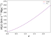 |
Fig. 1. Comparison between H(z) in standard ΛCDM and the one calculated by Eq. (8). H0 = H0, zi = 70 km s−1 Mpc−1, Ωk0 = 0, and Ωm0 = 0.3 are assumed. |
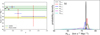 |
Fig. 2. Fitting results of H0(z) in the Pantheon+ sample case for six redshift bins. The left panel shows the value of H0(z) as a function of redshift. There is a clear decreasing trend. The green line gives H0 = 73.04 ± 1.04 km s−1 Mpc−1 from local distance ladder and its 1σ uncertainty (Riess et al. 2022). The yellow line is the value of H0 = 67.4 ± 0.5 km s−1 Mpc−1 from CMB measurements and its 1σ uncertainty (Planck Collaboration VI 2020). The right panel shows the normalized probability distributions of H0, z in six redshift bins. These distributions are almost Gaussian. |
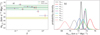 |
Fig. 3. Fitting results of H0(z) in the equal-number case for nine redshift bins. The left panel shows the value of H0(z) as a function redshift. There is a clear decreasing trend with 3.8σ significance at z > 0.3. The green line gives H0 = 73.04 ± 1.04 km s−1 Mpc−1 from the local distance ladder and its 1σ uncertainty (Riess et al. 2022). The yellow line is the value of H0 = 67.4 ± 0.5 km s−1 Mpc−1 from the CMB measurements and its 1σ uncertainty (Planck Collaboration VI 2020). The right panel shows the normalized probability distributions of H0, z in nine redshift bins. These distributions are almost Gaussian. |
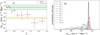 |
Fig. 4. Fitting results of H0(z) in the equal-width case for ten redshift bins. The left panel shows the value of H0(z) as a function redshift. There is a clear decreasing trend with 5.6σ significance at z > 0.3. The green line gives H0 = 73.04 ± 1.04 km s−1 Mpc−1 from local distance ladder and its 1σ uncertainty (Riess et al. 2022). The yellow line is the value of H0 = 67.4 ± 0.5 km s−1 Mpc−1 from CMB measurements and its 1σ uncertainty (Planck Collaboration VI 2020). The right panel shows the normalized probability distributions of H0, z in ten redshift bins. These distributions are almost Gaussian. |
By assuming the value H0, z is a constant in each redshift bin, previous works have directly used Eq. (6) to derive H0, z (Krishnan et al. 2020; Dainotti et al. 2021). First, this approach violates the assumption that the value of H0, z is constant in each bin. Equation (6) actually specifies that the value of H0, z is constant from z = 0 to z = zi and not from z = zi − 1 to z = zi. Therefore, the assumption leads H0, z as a constant from z = 0 to each z = zi. During the process of fitting the data in the ith redshift bin, the derived value of H0 is in the redshift range 0 − zi, not the value of H0, zi in zi − 1 − zi. Their measured H0, zi is not the value in the ith redshift bin. Thus, it is problematic to use the result to represent the value of H0, z in the ith redshift bin. Second, the correlation among each H0, zi was not considered in previous works. Due to the fact that the Hubble parameter and luminosity distance depend on the summation and the integration over redshifts, the value of H0, zi in low-redshift bins will affect the value in high-redshift bins. In our method, Eq. (8) reveals the redshift-evolution of H0(z). The most obvious difference between these two methods is that Eq. (6) demonstrates the value of H0, z from z = 0 to z = zi, but Eq. (8) reveals the value of H0, z at the ith redshift bin. The correlations can be removed by the principal component analysis.
When estimating cosmological parameters, we used the χ2 statistic for a particular model with the parameter set of θ (H0, zi):
with
![$$ \begin{aligned} \chi _{H(z)}^{2}=\sum _{i=1}^{N} \frac{\left[H_{\mathrm{obs} }\left(z_{i}\right)-H_{\mathrm{th} }\left(z_{i}\right)\right]^{2}}{\sigma ^{2}_i}, \end{aligned} $$](/articles/aa/full_html/2023/06/aa46356-23/aa46356-23-eq13.gif)
where Hobs(zi) and σi are the observed Hubble parameter and the corresponding 1σ error. Then, Hth(zi) is the value calculated from Eq. (8).
The value of  is
is
![$$ \begin{aligned} \chi _{\rm BAO}^{2}= \left[\nu _{\mathrm{obs} }\left(z_{i}\right)-\nu _{\mathrm{th} }\left(z_{i}\right)\right]\mathbf C_{BAO} ^{-1}\left[\nu _{\mathrm{obs} }\left(z_{i}\right)-\nu _{\mathrm{th} }\left(z_{i}\right)\right]^\mathrm{T}, \end{aligned} $$](/articles/aa/full_html/2023/06/aa46356-23/aa46356-23-eq15.gif)
where νobs is the vector of the BAO measurements at each redshift z (i.e., DV(rs, fid/rs), DM/rs, DH/rs, DA/rs). The comoving distance DM(z) is:

where DA(z) is the angular size distance. The radial BAO projection DH(z) is:
The angle-averaged distance DV(z) is
![$$ \begin{aligned} D_V(z) = \left[czD^2_M(z)/H(z)\right]^{1/3}. \end{aligned} $$](/articles/aa/full_html/2023/06/aa46356-23/aa46356-23-eq18.gif)
The sound horizon of the fiducial model is rs, fid = 147.5 Mpc.
The full covariance matrix of the Pantheon+ SNe Ia sample is considered in the process of calculating  (Scolnic et al. 2022). This covariance 1701×1701 matrix CSNe is defined as
where Dstat is the statistical matrix and Csys is the systematic covariance matrix. The value of  is:
is:
![$$ \begin{aligned} \chi _{\rm SNe}^{2}= \left[\mu _{\mathrm{obs} }\left(z_{i}\right)-\mu _{\mathrm{th} }\left(z_{i}\right)\right]\mathbf C _{\rm SNe}^{-1}\left[\mu _{\mathrm{obs} }\left(z_{i}\right)-\mu _{\mathrm{th} }\left(z_{i}\right)\right]^\mathrm{T} .\end{aligned} $$](/articles/aa/full_html/2023/06/aa46356-23/aa46356-23-eq22.gif)
The parameter μobs(zi) is the distance module from the Pantheon+ sample. The theoretical distance modulus, μth, is defined as
Taking Hth(z) from Eq. (8), the luminosity distance, dL, is expressed as
The constraints are derived by the Markov chain Monte Carlo (MCMC) code emcee (Foreman-Mackey et al. 2013). The adopted prior is H0 ∈ [50,80] km s−1 Mpc−1 for all H0, zi. Observations of SNe Ia and CMB set tight constraints on the cosmic matter density Ωm0, which are both around 0.3 (Brout et al. 2022; Planck Collaboration VI 2020). Thus, a fiducial value Ωm0 = 0.3 for cosmic matter density was used during the fitting process. We repeated our analysis with the Gaussian prior Ωm0 = 0.315 ± 0.007 from Planck CMB measurements (Planck Collaboration VI 2020) and found that it gives very similar results. Thus, the results are largely insensitive to the choice of either prior.
3.2. Principal-component analysis of H0, z
Although each redshift bin is treated as independent during the fitting process, the results of H0, zi are still correlated. This is expected, as the integration and summation over low-redshift bins in Eq. (8) definitely affects the model fit in the middle and higher redshift bins. In order to remove these correlations, we calculate the transformation matrix (Huterer & Cooray 2005). The principal component analysis presents a compressed form of the result with all information about the constraint from observations.
The fitting results impose constraints on the parameters H0, zi(i = 1…N). The covariance matrix can be generated by taking the average over the chain, namely,
where H is a vector with components H0, zi and HT is the transpose. We transformed the covariance matrix to decorrelate the H0, zi estimations (Huterer & Cooray 2005). This was achieved by finding the uncorrelated basis by diagonalizing the inverse covariance matrix. The Fisher matrix is defined as
where the matrix Λ is the diagonalized covariance for transformed bins. The transformation matrix T is used as the square root of the Fisher matrix, which is defined as

One advantage of this method is that the rows of T are almost positive across all bands. After being normalized, the rows of T which means the weights for H0, zi sum to unity. Finally, it is clear that the new parameters,

are uncorrelated, because they have the covariance matrix Λ−1.
After the correlations among H0, z are removed, the corner plots of H0, z are shown in supplementary Figs. 5 and 6 for the equal-number binning case and equal-width binning case, respectively. The constraints on H0, z are tight and the probability distributions are almost Gaussian.
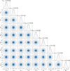 |
Fig. 5. Corner plot of H0, z values from the MCMC code for the equal-number binning case. The panels on the diagonal show the 1D histogram for each parameter obtained by marginalizing over the other parameters. These distributions are almost Gaussian. The off-diagonal panels show two-dimensional projections of the posterior probability distributions for each pair of parameters, with contours to indicate 1σ–3σ confidence levels. |
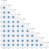 |
Fig. 6. Corner plot of H0, z values from the MCMC code for the equal-width binning case. The panels on the diagonal show the 1D histogram for each parameter obtained by marginalizing over the other parameters. These distributions are almost Gaussian. The off-diagonal panels show two-dimensional projections of the posterior probability distributions for each pair of parameters, with contours to indicate 1σ–3σ confidence levels. |
4. Results
4.1. SN Ia sample
Before the final result, we estimated the possible evolutionary trend only with the Pantheon+ sample. The whole sample contains 1701 data, most of which are located at low redshift. Therefore, we chose six bins with the upper boundaries of zi = 0.1, 0.2, 0.3, 0.6, 1.0, 2.4. On account of the relatively few data points in high-redshift bins, some intervals have to be loose. The value of H0, z as a function of redshift (panel a) and the normalized probability distributions (panel b) are shown in Fig. 2. The decreasing trend is clear at z > 0.3, but the scarce data in high-redshift bins give poor constraints. The 1σ uncertainties for high-redshift bins are so large that we decided to add the observed Hubble parameter data and BAO data (Yu et al. 2018; Cao & Ratra 2022). The joint dataset gives a strict constraint and can be used to research the evolution by different binning methods.
4.2. Two binning methods
Two redshift-binning methods were adopted. The first one is equal-number method, namely, the number of data points in each bin is almost equal (Dainotti et al. 2021). In contrast, the second one is equal-width method, namely, the bins are equally spaced in redshift (Huterer & Cooray 2005). For the equal-number method, we chose nine bins with the upper boundaries of zi = 0.0122, 0.025, 0.037, 0.108, 0.199, 0.267, 0.350, 0.530, and 2.40. Each bin contains about 194 data points (listed in Table 3). More binnings were also performed and we find that the likelihood distributions of H0, z for some bins deviate from Gaussian, due to the scarcity of data points in some high-redshift bins. In the case of non-Gaussian H0, z distributions, the decorrelation process may introduce some biases. Therefore, nine bins were adopted.
Fitting results of H0, zi (in units of km s−1 Mpc−1) in the equal-number case.
Altogether, there are nine free parameters in the MCMC approach, namely, H0, z1, …, H0, z9. The Pantheon+ SNe Ia sample (Scolnic et al. 2022), BAO data and observed Hubble parameter data were used to estimate the value of H0, z (see Sect. 3). Given this joint dataset, we used the MCMC code emcee (Foreman-Mackey et al. 2013) to sample the parameter set θ (H0, zi). The prior of H0 ∈ [50,80] km s−1 Mpc−1 for all H0, zi was adopted. After removing the correlation among H0, z by diagonalizing the covariance matrix (see Methods), the best-fit results are shown in Table 3. The value of H0, z as a function of redshift (panel a) and the normalized probability distributions (panel b) are shown in Fig. 3. Due to the large number of data in each bin and a fixed Ωm0, the uncertainty of H0, z is less than 1.0, which is consistent with previous work (Dainotti et al. 2021; Wang 2022b). In the first seven bins, the fitting results are nearly constant and the value is consistent with the one derived by the local distance ladder (Riess et al. 2022), however, it drops rapidly thereafter. It is worth noting that the result in the last bin is consistent with the value from Planck measurements at a 2σ confidence level (Planck Collaboration VI 2020).
There is an apparent decreasing trend in H0(z) as a function of redshift. To quantify the significance of this trend, we used the null hypothesis method (Wong et al. 2020; Millon et al. 2020). The hypothesis in this situation posits that the values of H0(z) in each redshift bin are consistent with each other. We first fit a linear regression through each redshift bin. Next, we generated sets of nine mock H0 values with their own uncertainty probability distribution centered around the value of H0 = 73.04 ± 1.04 km s−1 Mpc−1 (Riess et al. 2022). The weight of each mock value was calculated as follows (Wong et al. 2020). First, the uncertainties’ probability distributions are rescaled so that their maximal values are equal to 1. Then, the area under each distribution is calculated and the areas are rescaled by their median. Last, the inverse square of the rescaled areas is taken as the weight for each mock value. We also fit a linear regression through the mock value. The slope of the data falls 3.8σ away from the mock slope distribution. In other words, the decreasing trend in H0(z) with increasing redshift has a significance of 3.8σ.
In the second case, the bins are equally spaced with a redshift-width 0.1 in the redshift range [0, 0.4]. Because there are so few data points from z = 0.4 to z = 2.4, wider intervals should be adopted in this range. We also tried to equally bin z with a width of 0.1 in the redshift range [0, 1.0]. The poor constraints in some intervals lead to biases in the decorrelation process. Finally, ten bins are adopted with the upper boundaries zi = 0.10, 0.20, 0.30, 0.40, 0.6, 0.8, 1.1, 1.5, 2.0, and 2.4. The number of data points and best-fit results are given in Table 4. The uncertainties of the constraints increase gradually as the number of data decreases. The value of H0, z as a function of redshift (panel a) and the normalized probability distributions of H0, z (panel b) are given in Fig. 4. The fitting results of the first three bins are consistent with the value from the local distance ladder within 1σ confidence level (Riess et al. 2022), and the last two bins are consistent with the value from Planck CMB measurements within 1σ confidence level (Planck Collaboration VI 2020). There is a gradually decreasing trend in H0(z) from the third bin to the last bin. Using the same method as above, the significance of the decreasing trend is 5.6σ. More importantly, the decreasing trend begins at the same redshift z ∼ 0.3 for the two binning methods.
Fitting results of H0, zi (in units of km s−1 Mpc−1) in the equal-width case.
Finally, we tested whether additional parameters to describe H0(z) are actually needed to improve on a flat ΛCDM model fit to the data. For the flat ΛCDM model, the same value of Ωm0 = 0.3 was adopted and H0 was left as a free parameter. Two kinds of standard information criteria were considered: Akaike information criterion (AIC; Akaike 1974) and the Bayesian information criterion (BIC; Schwarz 1978). Their definitions are: AIC = −2lnL + 2k, and BIC = −2lnL + klnn, where L ∝ e−χ2/2 is the value of the maximum likelihood function, k is the number of model parameters, and n = 1746 is the total number of data points. From Table 5, there is a significant improvement for both binning methods relative to the flat ΛCDM model, with ΔAIC of −44.49 and −37.41, ΔBIC of 0.77 and −11.77 for equal-number and equal-width binning methods, respectively. Thus, these values are sufficient to favor the H0(z) model over ΛCDM.
Model comparison.
5. Conclusions
We constrained H0, z, defined as the value of H0 derived from the cosmic observations at redshift z, and its variation as a function of redshift using a non-parametric approach. The correlations among H0, z were removed by diagonalizing the covariance matrix. A decreasing trend in H0, z with a significance of 3.8σ and 5.6σ was found for equal-number and equal-width binning methods, respectively. At low redshift, the value of H0, z is consistent with the value from the local distance ladder and it decreases to the value from CMB measurements at high redshift. The evolution of H0, z can effectively relieve the Hubble tension without modifications of early Universe physics. The descending trend may be a signal for the flat ΛCDM model is breaking down (Krishnan et al. 2021, 2022).
The decreasing behavior found for the Hubble constant with the redshift is significant and urgently calls for an explanation. At present, the physical mechanism behind the decreasing trend in H0, z is unclear. Two possible origins are suggested by the systematic uncertainties in the data and modifications of the standard cosmological model. For the systematic uncertainties, it has been found that the light-curve parameters of SNe Ia, such as the stretch and the color, show no clear dependence on the redshift for the Pantheon SNe Ia sample (Scolnic et al. 2018). However, a recent study found that the SNe Ia SALT2.4 light-curve stretch distribution evolves as a function of redshift (Nicolas et al. 2021), which will affect the value of Hubble constant derived from SNe Ia. Thus, the redshift-dependence of SNe Ia parameters should be extensively studied. If it is not due to selection effects or systematic uncertainties in the data, our results should be interpreted with physical models. This might indicate the emergence of new physics (Di Valentino et al. 2021; Shah et al. 2021), such as dynamical dark energy (Zhao et al. 2017) or modified gravity models (Kazantzidis & Perivolaropoulos 2020; Dainotti et al. 2021). From the Pantheon+ SNe Ia sample, marginal evidence of an increase of cosmic matter density, Ωm0, with a minimum redshift was discovered (Brout et al. 2022), which supports the decreasing trend in the Hubble constant found in this paper. Moreover, a dynamical dark energy signal with 2σ confidence level was found from Pantheon+ sample (Wang 2022a). Due to the lack of high-redshift data, the redshift bins are sparse at z > 0.5 and H0, z can only be measured below z = 2.4. In the future, constraints placed on H0, z will improve significantly with upcoming cosmological observations, such as the James Webb Space Telescope, Large Synoptic Survey Telescope, and Euclid and Nancy Grace Roman Space Telescope. In particular, γ-ray bursts and fast radio bursts may shed light on the evolution of H0, z (Wang et al. 2015, 2022; Khadka & Ratra 2020; Cao et al. 2022; Liang et al. 2022; Dainotti et al. 2022b; Luongo & Muccino 2023; Wu et al. 2022).
Acknowledgments
We appreciate the referee for valuable comments and suggestions, which have helped to improve this manuscript. This work was supported by the National Natural Science Foundation of China (grant No. 12273009), the China Manned Spaced Project (CMS-CSST-2021-A12), and the Jiangsu Funding Program for Excellent Postdoctoral Talent (20220ZB59). The numerical code can be found in the GitHub repository (https://github.com/JoJo20221003/Hz-Code).
References
- Abbott, T. M. C., Abdalla, F. B., Alarcon, A., et al. 2019, MNRAS, 483, 4866 [NASA ADS] [CrossRef] [Google Scholar]
- Akaike, H. 1974, IEEE Trans. Auto. Control, 19, 716 [Google Scholar]
- Alam, S., Aubert, M., Avila, S., et al. 2021, Phys. Rev. D, 103, 083533 [NASA ADS] [CrossRef] [Google Scholar]
- Bautista, J. E., Paviot, R., Vargas Magaña, M., et al. 2021, MNRAS, 500, 736 [Google Scholar]
- Benetti, M., Capozziello, S., & Lambiase, G. 2021, MNRAS, 500, 1795 [Google Scholar]
- Bernal, J. L., Verde, L., & Riess, A. G. 2016, J. Cosmol. Astropart. Phys., 2016, 019 [CrossRef] [Google Scholar]
- Borghi, N., Moresco, M., & Cimatti, A. 2022, ApJ, 928, L4 [NASA ADS] [CrossRef] [Google Scholar]
- Brout, D., Scolnic, D., Popovic, B., et al. 2022, ApJ, 938, 110 [NASA ADS] [CrossRef] [Google Scholar]
- Cai, R.-G., Guo, Z.-K., Li, L., Wang, S.-J., & Yu, W.-W. 2021, Phys. Rev. D, 103, L121302 [CrossRef] [Google Scholar]
- Cao, S., & Ratra, B. 2022, MNRAS, 513, 5686 [Google Scholar]
- Cao, S., Dainotti, M., & Ratra, B. 2022, MNRAS, 512, 439 [NASA ADS] [CrossRef] [Google Scholar]
- Capozziello, S., & Fang, L. Z. 2002, Int. J. Mod. Phys. D, 11, 483 [NASA ADS] [CrossRef] [Google Scholar]
- Carter, P., Beutler, F., Percival, W. J., et al. 2018, MNRAS, 481, 2371 [NASA ADS] [CrossRef] [Google Scholar]
- Colgáin, E., Sheikh-Jabbari, M. M., Solomon, R., Dainotti, M. G., & Stojkovic, D. 2022, ApJ, submitted [arXiv:2206.11447] [Google Scholar]
- Dainotti, M. G., De Simone, B., Schiavone, T., et al. 2021, ApJ, 912, 150 [NASA ADS] [CrossRef] [Google Scholar]
- Dainotti, M. G., De Simone, B. D., Schiavone, T., et al. 2022a, Galaxies, 10, 24 [NASA ADS] [CrossRef] [Google Scholar]
- Dainotti, M. G., Nielson, V., Sarracino, G., et al. 2022b, MNRAS, 514, 1828 [CrossRef] [Google Scholar]
- Di Valentino, E., Mena, O., Pan, S., et al. 2021, Class. Quant. Grav., 38, 153001 [NASA ADS] [CrossRef] [Google Scholar]
- du Mas des Bourboux, H., Rich, J., Font-Ribera, A., et al. 2020, ApJ, 901, 153 [CrossRef] [Google Scholar]
- Foreman-Mackey, D., Hogg, D. W., Lang, D., & Goodman, J. 2013, PASP, 125, 306 [Google Scholar]
- Gil-Marín, H., Bautista, J. E., Paviot, R., et al. 2020, MNRAS, 498, 2492 [Google Scholar]
- Haslbauer, M., Banik, I., & Kroupa, P. 2020, MNRAS, 499, 2845 [Google Scholar]
- Hou, J., Sánchez, A. G., Ross, A. J., et al. 2021, MNRAS, 500, 1201 [Google Scholar]
- Hu, J. P., & Wang, F. Y. 2022, MNRAS, 517, 576 [NASA ADS] [CrossRef] [Google Scholar]
- Hu, J.-P., & Wang, F.-Y. 2023, Universe, 9, 94 [CrossRef] [Google Scholar]
- Huterer, D., & Cooray, A. 2005, Phys. Rev. D, 71, 023506 [NASA ADS] [CrossRef] [Google Scholar]
- Jia, X. D., Hu, J. P., Yang, J., Zhang, B. B., & Wang, F. Y. 2022, MNRAS, 516, 2575 [Google Scholar]
- Jiao, K., Borghi, N., Moresco, M., & Zhang, T.-J. 2023, ApJS, 265, 48 [NASA ADS] [CrossRef] [Google Scholar]
- Jimenez, R., & Loeb, A. 2002, ApJ, 573, 37 [NASA ADS] [CrossRef] [Google Scholar]
- Jimenez, R., Verde, L., Treu, T., & Stern, D. 2003, ApJ, 593, 622 [NASA ADS] [CrossRef] [Google Scholar]
- Kazantzidis, L., & Perivolaropoulos, L. 2020, Phys. Rev. D, 102, 023520 [Google Scholar]
- Kenworthy, W. D., Scolnic, D., & Riess, A. 2019, ApJ, 875, 145 [NASA ADS] [CrossRef] [Google Scholar]
- Khadka, N., & Ratra, B. 2020, MNRAS, 499, 391 [NASA ADS] [CrossRef] [Google Scholar]
- Kreisch, C. D., Cyr-Racine, F.-Y., & Doré, O. 2020, Phys. Rev. D, 101, 123505 [Google Scholar]
- Krishnan, C., Colgáin, E. Ó., Ruchika, Sen., et al. 2020, Phys. Rev. D, 102, 103525 [NASA ADS] [CrossRef] [Google Scholar]
- Krishnan, C., Mohayaee, R., Colgáin, E. Ó., Sheikh-Jabbari, M. M., & Yin, L. 2021, Class. Quant. Grav., 38, 184001 [NASA ADS] [CrossRef] [Google Scholar]
- Krishnan, C., Mohayaee, R., Colgáin, E. Ã., Sheikh-Jabbari, M. M., & Yin, L. 2022, Phys. Rev. D, 105, 063514 [NASA ADS] [CrossRef] [Google Scholar]
- Krishnan, C., & Mondol, R. 2022, ApJ, submitted [arXiv:2201.13384] [Google Scholar]
- Liang, N., Li, Z., Xie, X., & Wu, P. 2022, ApJ, 941, 84 [CrossRef] [Google Scholar]
- Luongo, O., & Muccino, M. 2023, MNRAS, 518, 2247 [Google Scholar]
- Malekjani, M., Mc Conville, R., Colgáin, E., Pourojaghi, S., & Sheikh-Jabbari, M. M. 2023, ApJ, submitted [arXiv:2301.12725] [Google Scholar]
- Marra, V., Amendola, L., Sawicki, I., & Valkenburg, W. 2013, Phys. Rev. Lett., 110, 241305 [NASA ADS] [CrossRef] [Google Scholar]
- Millon, M., Galan, A., Courbin, F., et al. 2020, A&A, 639, A101 [NASA ADS] [CrossRef] [EDP Sciences] [Google Scholar]
- Moresco, M. 2015, MNRAS, 450, L16 [NASA ADS] [CrossRef] [Google Scholar]
- Moresco, M., Cimatti, A., Jimenez, R., et al. 2012, J. Cosmol. Astropart. Phys., 2012, 006 [Google Scholar]
- Moresco, M., et al. 2016, J. Cosmol. Astropart. Phys., 2016, 014 [CrossRef] [Google Scholar]
- Naidoo, K., Jaber, M., Hellwing, W. A., & Bilicki, M. 2022, ApJ, submitted [arXiv:2209.08102] [Google Scholar]
- Neveux, R., Burtin, E., de Mattia, A., et al. 2020, MNRAS, 499, 210 [NASA ADS] [CrossRef] [Google Scholar]
- Nicolas, N., Rigault, M., Copin, Y., et al. 2021, A&A, 649, A74 [NASA ADS] [CrossRef] [EDP Sciences] [Google Scholar]
- Colgáin, Ó. E., Sheikh-Jabbari, M. M., Solomon, R., et al. 2022, Phys. Rev. D, 106, L041301 [CrossRef] [Google Scholar]
- Perivolaropoulos, L., & Skara, F. 2022, New Astron. Rev., 95, 101659 [CrossRef] [Google Scholar]
- Planck Collaboration VI. 2020, A&A, 641, A6 [Google Scholar]
- Poulin, V., Smith, T. L., Karwal, T., & Kamionkowski, M. 2019, Phys. Rev. Lett., 122, 221301 [Google Scholar]
- Ratsimbazafy, A. L., Loubser, S. I., Crawford, S. M., et al. 2017, MNRAS, 467, 3239 [NASA ADS] [CrossRef] [Google Scholar]
- Rezazadeh, K., Ashoorioon, A., & Grin, D. 2022, ApJ, submitted [arXiv:2208.07631] [Google Scholar]
- Riess, A. G. 2020, Nat. Rev. Phys., 2, 10 [NASA ADS] [CrossRef] [Google Scholar]
- Riess, A. G., Strolger, L.-G., Casertano, S., et al. 2007, ApJ, 659, 98 [NASA ADS] [CrossRef] [Google Scholar]
- Riess, A. G., Yuan, W., Macri, L. M., et al. 2022, ApJ, 934, L7 [NASA ADS] [CrossRef] [Google Scholar]
- Sakstein, J., & Trodden, M. 2020, Phys. Rev. Lett., 124, 161301 [CrossRef] [Google Scholar]
- Schöneberg, N., Abellán, G. F., Sánchez, A. P., et al. 2022, Phys. Rep., 984, 1 [CrossRef] [Google Scholar]
- Schwarz, G. 1978, Ann. Stat., 6, 461 [Google Scholar]
- Scolnic, D. M., Jones, D. O., Rest, A., et al. 2018, ApJ, 859, 101 [NASA ADS] [CrossRef] [Google Scholar]
- Scolnic, D., Brout, D., Carr, A., et al. 2022, ApJ, 938, 113 [NASA ADS] [CrossRef] [Google Scholar]
- Shah, P., Lemos, P., & Lahav, O. 2021, A&ARv, 29, 9 [NASA ADS] [CrossRef] [Google Scholar]
- Simon, J., Verde, L., & Jimenez, R. 2005, Phys. Rev. D, 71, 123001 [NASA ADS] [CrossRef] [Google Scholar]
- Stern, D., Jimenez, R., Verde, L., Kamionkowski, M., & Stanford, S. A. 2010, J. Cosmol. Astropart. Phys., 2010, 008 [CrossRef] [Google Scholar]
- Vagnozzi, S. 2021, Phys. Rev. D, 104, 063524 [NASA ADS] [CrossRef] [Google Scholar]
- Verde, L., Treu, T., & Riess, A. G. 2019, Nat. Astron., 3, 891 [Google Scholar]
- Wang, D. 2022a, Phys. Rev. D, 106, 063515 [NASA ADS] [CrossRef] [Google Scholar]
- Wang, D. 2022b, ApJ, submitted [arXiv:2207.10927] [Google Scholar]
- Wang, F. Y., Dai, Z. G., & Liang, E. W. 2015, New Astron. Rev., 67, 1 [CrossRef] [Google Scholar]
- Wang, F. Y., Hu, J. P., Zhang, G. Q., & Dai, Z. G. 2022, ApJ, 924, 97 [NASA ADS] [CrossRef] [Google Scholar]
- Wong, K. C., Suyu, S. H., Chen, G. C.-F., et al. 2020, MNRAS, 498, 1420 [Google Scholar]
- Wong, J. H. W., Shanks, T., Metcalfe, N., & Whitbourn, J. R. 2022, MNRAS, 511, 5742 [NASA ADS] [CrossRef] [Google Scholar]
- Wu, Q., Zhang, G.-Q., & Wang, F.-Y. 2022, MNRAS, 515, L1 [NASA ADS] [CrossRef] [Google Scholar]
- Yu, H., Ratra, B., & Wang, F.-Y. 2018, ApJ, 856, 3 [NASA ADS] [CrossRef] [Google Scholar]
- Zhang, C., Zhang, H., Yuan, S., et al. 2014, RAA, 14, 1221 [NASA ADS] [Google Scholar]
- Zhao, G.-B., Raveri, M., Pogosian, L., et al. 2017, Nat. Astron., 1, 627 [NASA ADS] [CrossRef] [Google Scholar]
All Tables
All Figures
|
Fig. 1. Comparison between H(z) in standard ΛCDM and the one calculated by Eq. (8). H0 = H0, zi = 70 km s−1 Mpc−1, Ωk0 = 0, and Ωm0 = 0.3 are assumed. |
| In the text | |
|
Fig. 2. Fitting results of H0(z) in the Pantheon+ sample case for six redshift bins. The left panel shows the value of H0(z) as a function of redshift. There is a clear decreasing trend. The green line gives H0 = 73.04 ± 1.04 km s−1 Mpc−1 from local distance ladder and its 1σ uncertainty (Riess et al. 2022). The yellow line is the value of H0 = 67.4 ± 0.5 km s−1 Mpc−1 from CMB measurements and its 1σ uncertainty (Planck Collaboration VI 2020). The right panel shows the normalized probability distributions of H0, z in six redshift bins. These distributions are almost Gaussian. |
| In the text | |
|
Fig. 3. Fitting results of H0(z) in the equal-number case for nine redshift bins. The left panel shows the value of H0(z) as a function redshift. There is a clear decreasing trend with 3.8σ significance at z > 0.3. The green line gives H0 = 73.04 ± 1.04 km s−1 Mpc−1 from the local distance ladder and its 1σ uncertainty (Riess et al. 2022). The yellow line is the value of H0 = 67.4 ± 0.5 km s−1 Mpc−1 from the CMB measurements and its 1σ uncertainty (Planck Collaboration VI 2020). The right panel shows the normalized probability distributions of H0, z in nine redshift bins. These distributions are almost Gaussian. |
| In the text | |
|
Fig. 4. Fitting results of H0(z) in the equal-width case for ten redshift bins. The left panel shows the value of H0(z) as a function redshift. There is a clear decreasing trend with 5.6σ significance at z > 0.3. The green line gives H0 = 73.04 ± 1.04 km s−1 Mpc−1 from local distance ladder and its 1σ uncertainty (Riess et al. 2022). The yellow line is the value of H0 = 67.4 ± 0.5 km s−1 Mpc−1 from CMB measurements and its 1σ uncertainty (Planck Collaboration VI 2020). The right panel shows the normalized probability distributions of H0, z in ten redshift bins. These distributions are almost Gaussian. |
| In the text | |
|
Fig. 5. Corner plot of H0, z values from the MCMC code for the equal-number binning case. The panels on the diagonal show the 1D histogram for each parameter obtained by marginalizing over the other parameters. These distributions are almost Gaussian. The off-diagonal panels show two-dimensional projections of the posterior probability distributions for each pair of parameters, with contours to indicate 1σ–3σ confidence levels. |
| In the text | |
|
Fig. 6. Corner plot of H0, z values from the MCMC code for the equal-width binning case. The panels on the diagonal show the 1D histogram for each parameter obtained by marginalizing over the other parameters. These distributions are almost Gaussian. The off-diagonal panels show two-dimensional projections of the posterior probability distributions for each pair of parameters, with contours to indicate 1σ–3σ confidence levels. |
| In the text | |
Current usage metrics show cumulative count of Article Views (full-text article views including HTML views, PDF and ePub downloads, according to the available data) and Abstracts Views on Vision4Press platform.
Data correspond to usage on the plateform after 2015. The current usage metrics is available 48-96 hours after online publication and is updated daily on week days.
Initial download of the metrics may take a while.