| Issue |
A&A
Volume 686, June 2024
|
|
|---|---|---|
| Article Number | A30 | |
| Number of page(s) | 8 | |
| Section | Cosmology (including clusters of galaxies) | |
| DOI | https://doi.org/10.1051/0004-6361/202348585 | |
| Published online | 28 May 2024 | |
Breaking the baryon-dark matter degeneracy in a model-independent way through the Sunyaev-Zeldovich effect
1
Scuola Superiore Meridionale, Largo S. Marcellino 10, 80138 Napoli, Italy
e-mail: annac.alfano@studenti.unina.it
2
Università di Camerino, Divisione di Fisica, Via Madonna delle carceri 9, 62032 Camerino, Italy
e-mail: orlando.luongo@unicam.it; marco.muccino@lnf.infn.it
3
SUNY Polytechnic Institute, 13502 Utica, New York, USA
4
INFN, Sezione di Perugia, Perugia 06123, Italy
5
INAF – Osservatorio Astronomico di Brera, Milano, Italy
6
Al-Farabi Kazakh National University, Al-Farabi av. 71, 050040 Almaty, Kazakhstan
Received:
13
November
2023
Accepted:
15
February
2024
Context. In cosmological fits, it is common to fix the baryon density ωb via the cosmic microwave background. We here constrain ωb by means of a model-independent interpolation of the acoustic parameter from correlated baryonic acoustic oscillations.
Aims. The proposed technique is used to alleviate the degeneracy between baryonic and dark matter abundances.
Methods. We propose a model-independent Bézier parametric interpolation and applied it to intermediate-redshift data. We first interpolated the observational Hubble data to extract cosmic bounds over the (reduced) Hubble constant h0 and interpolated the angular diameter distances, D(z), of the galaxy clusters, inferred from the Sunyaev-Zeldovich effect, to constrain the spatial curvature, Ωk. Through the Hubble points and D(z) determined in this way, we interpolated uncorrelated data of baryonic acoustic oscillations bounding the baryon ωb and total matter ωm densities, reinforcing the constraints on h0 and Ωk with the same technique. Finally, to remove the matter sector degeneracy, we obtained ωb by interpolating the acoustic parameter from correlated baryonic acoustic oscillations.
Results. Monte Carlo Markov chain simulations agree at 1σ confidence level with the flat ΛCDM model and are roughly suitable at 1σ with its nonflat extension, while the Hubble constant appears in tension up to the 2σ confidence levels.
Conclusions. Our method excludes very small extensions of the standard cosmological model, and on the Hubble tension side, seems to match local constraints slightly.
Key words: cosmological parameters / cosmology: theory / dark matter / dark energy / early Universe / large-scale structure of Universe
© The Authors 2024
 Open Access article, published by EDP Sciences, under the terms of the Creative Commons Attribution License (https://creativecommons.org/licenses/by/4.0), which permits unrestricted use, distribution, and reproduction in any medium, provided the original work is properly cited.
This article is published in open access under the Subscribe to Open model. Subscribe to A&A to support open access publication.
1. Introduction
In the standard cosmological puzzle, the accelerated expansion of the Universe represents solid evidence, first detected by means of type Ia supernovae (SNe Ia) observations (Riess et al. 1998; Perlmutter et al. 1999). The presence of dust in the form of baryons and (cold) dark matter alone is not capable of accelerating the Universe today, remarkable exceptions are unified models of dark energy, in which dark energy emerges as a consequence of dark matter (see, e.g., Boshkayev et al. 2019 and references therein). Accordingly, the acceleration of the Universe can be attributed to an exotic dark energy fluid that exerts a repulsive gravitational effect through its negative equation-of-state parameter (Sahni & Starobinsky 2000; Copeland et al. 2006; Tsujikawa et al. 2011).
The energy momentum budget of the Universe contains a dark energy contribution of ∼70%, and the remaining ∼30% consists of cold dark matter (CDM) and baryonic matter (Planck Collaboration VI 2020). Within the current cosmological background scenario, the ΛCDM model, it is not possible to measure baryonic matter and cold dark matter separately by relying on SNe Ia observations alone. This limitation is not only a characteristic of the current cosmological background scenario, where dark energy is in the form of the cosmological constant Λ (Carroll 2001), but of any dark energy scenario. However, of all possible frameworks, the ΛCDM model remains the most statistically favored approach to describe the large scale dynamics of the Universe, but it is plagued by conceptual inconsistencies.
Specifically, the ΛCDM paradigm still has coincidence and fine-tuning problems (Copeland et al. 2006) and cosmological tensions related to discrepancies in the Hubble constant measurements and to the amplitude of the clustering of matter S8 using high- and low-redshift probes (Bernal & Libanore 2023; Di Valentino et al. 2021; Abdalla et al. 2022). To overcome these issues, several theoretical efforts have been made to find alternative models that reproduce the successful features of the ΛCDM paradigm (Luongo & Muccino 2018; D’Agostino et al. 2022; Belfiglio et al. 2022).
From a phenomenological standpoint, diverse model-independent approaches have been proposed to estimate the cosmological parameters without assuming the cosmological model a priori (Capozziello et al. 2013; Dunsby & Luongo 2016; Luongo & Muccino 2021b, 2023; Shafieloo 2007; Shafieloo & Clarkson 2010; Haridasu et al. 2018).
Motivated by the need of disentangling baryons from cold dark matter, we here propose a joint fitting procedure based on the model-independent approach of the Bézier parametric interpolation, which
a) Approximates the Hubble rate H(z) via the observational Hubble data (OHD) and constrains the reduced Hubble constant h0 (Amati et al. 2019),
b) Uses the approximated H(z) to interpolate the D(z) of galaxy clusters and provide bounds on the spatial curvature Ωk, and
c) Employs the above-extrapolated H(z) and D(z) to fit both uncorrelated and correlated baryonic acoustic oscillations (BAO) data to constrain the matter densities of baryons Ωb and all matter components Ωm, via  and
and  , on which the comoving sound horizon, rs, depends (Aizpuru et al. 2021).
Steps a)–c) are performed jointly to constrain the parameters h0, Ωk, ωb, and ωm in a single fit.
We point out that the correlated BAO is essential to break the degeneracy between ωb and ωm (Efstathiou & Bond 1999). This is different from the standard procedure fixing ωb to the cosmic microwave background (CMB) value (Planck Collaboration VI 2020). Accordingly, we intentionally neglected the CMB data from the Planck satellite and the Pantheon catalog of SNe Ia (Scolnic et al. 2018) because their determination of h0 differs. The results of our Monte Carlo Markov chain (MCMC) simulations, based on the Metropolis-Hastings algorithm, suggest that the matter sector degeneracy is likely alleviated without the need for CMB and/or SNe Ia data. Notably, this technique, while valuable, does not completely eliminate the cosmic tensions that still persist. In the flat scenario, our h0 agrees well with the Planck estimates (Planck Collaboration VI 2020), but is still barely consistent with SNe Ia (Riess et al. 2022) at the 1σ confidence level, while in the nonflat case, our h0 is consistent with Planck only at the 2σ confidence level (Planck Collaboration VI 2020). This indicates that the spatial curvature may influence the h0 measurements, as has been pointed out in the literature and agrees with our results (see, e.g., Liu et al. 2022; Li et al. 2020; Zhang et al. 2023). Consequently, when comparing our results with expectations based on the flat (nonflat) ΛCDM framework, we obtain constraints that agree well with the standard cosmological model at the 1σ (2σ) level. This confirms that the ΛCDM paradigm is still supported within our treatment.
The paper is structured as follows. In Sect. 2, we introduce the data sets and show how to use them to perform model-independent interpolations through Bézier curves. In Sect. 3, we show the numerical constraints on h0, Ωk, ωb and ωm obtained from our MCMC analysis and compare them with the best-fit parameters inferred from the flat and nonflat ΛCDM models. In Sect. 4, we summarize the physical implications of our efforts, and we report our conclusions and perspectives.
2. Methods
To obtain model-independent constraints on the key cosmological parameters, we used intermediate-redshift catalogs, such as OHD, galaxy clusters, and BAO data sets. The Pantheon catalog of SNe Ia (Scolnic et al. 2018) and CMB data from the Planck satellite (Planck Collaboration VI 2020) were intentionally excluded in view of the existing difference in their estimates of h0 (Riess et al. 2022; Planck Collaboration VI 2020).
The model-independent technique we used is based on the well-established Bézier parametric interpolation, which was first introduced in Luongo & Muccino (2021b) and is widely adopted in cosmological contexts with promising results (Amati et al. 2019; Montiel et al. 2021; Luongo & Muccino 2023; Muccino et al. 2023). We employed this technique in a joint fitting procedure to
-
Interpolate H(z) from OHD (Jimenez & Loeb 2002),
-
Use it to derive the D(z) of galaxy clusters and BAO observables, and
-
Interpolate BAO data to break the baryonic–dark matter degeneracy.
It is worth stressing that the H(z) and D(z) interpolated in this bear no a priori assumptions on Ωk as long as the data sets do not carry specific priors on it.
2.1. Hubble rate model-independent reconstruction via Bézier polynomials
We interpolated the most recently updated sample of NO = 33 OHD, spanning up to a maximum redshift of zm = 1.965 (see Table 1). These measurements were determined from spectroscopic measurements of the differences in age Δt and redshift Δz of pairs of passively evolving galaxies (formed at the same time) based on the identity H(z) = − (1 + z)−1Δz/Δt (Jimenez & Loeb 2002).
Redshift distribution (first column) of the OHD measurements with the statistical errors (second column) and the reference papers (third column).
The systematic errors associated with OHD mostly depend upon stellar population synthesis models and libraries and on the initial mass functions used to calibrate the measurement, together with the stellar metallicity of the population. They contribute an additional 20–30% error to the determination of H(z) and h0 (Montiel et al. 2021; Moresco et al. 2022; Muccino et al. 2023).
The best-fit, nonlinear, and monotonic growing function with redshift of these data is a second-order Bézier curve with coefficients αi (Amati et al. 2019; Luongo & Muccino 2021b; Montiel et al. 2021; Luongo & Muccino 2023; Muccino et al. 2023), that is,
where we defined gα = 100 km s−1 Mpc−1. This interpolated function can also be extrapolated beyond zm to cover the redshift range of the other intermediate-redshift probes that we introduce below.
Fitting the OHD measurements with Eq. (1) provides a model-independent estimate of the dimensionless Hubble constant because at z = 0, H0/gα ≡ h0 ≡ α0.
For Gaussian-distributed errors σHk, the coefficients αi are found by maximizing the log-likelihood function
![$$ \begin{aligned} \ln \mathcal{L} _{\rm O} = -\frac{1}{2} \sum _{j=1}^{N_{\rm O}}\left\{ \left[\dfrac{H_j-H_2(z_j)}{\sigma _{H_j}}\right]^2 + \ln (2\pi \sigma ^2_{H_j})\right\} . \end{aligned} $$](/articles/aa/full_html/2024/06/aa48585-23/aa48585-23-eq4.gif)
2.2. Constraining the curvature with SZ data
The Sunyaev-Zeldovich (SZ) effect (Sunyaev & Zeldovich 1970, 1972) is the spectral distortion of the CMB photons via inverse-Compton scattering by high-energy electron gas in galaxy clusters (Carlstrom et al. 2002). While CMB photons are observed at microwave frequencies, the intracluster electrons are observed in the X-rays due to thermal Bremsstrahlung emission.
Combining the SZ effect, which is redshift independent, with the X-ray surface brightness of the intracluster gas, which is redshift dependent, we obtained the angular diameter distance to galaxy clusters. For X-ray observations with a relatively high threshold signal-to-noise ratio, it is possible to determine the triaxial structure of the clusters, and thus, their morphology-corrected diameter angular distances D(z). A sample of NS = 25 clusters with these determined distances (De Filippis et al. 2005) is listed in Table 2. All these measurements are affected by systematic errors due to the presence of radio halos, which can mask the temperature decrement of the SZ effect, the X-ray absolute flux, the electron temperature calibrations, and the SZ effect calibration itself (Bonamente et al. 2006), whereas the determination of the trixial shape has a negligible impact (De Filippis et al. 2005). The typical errors are ≈13%.
Sample of galaxy clusters with redshift (first column) and diameter angular distances (second column), taken from De Filippis et al. (2005).
Using Eq. (1), we obtained an interpolated angular diameter distance that is defined as
![$$ \begin{aligned} D_2(z) = \frac{c\left(1+z\right)^{-1}}{g_\alpha \alpha _0\sqrt{\Omega _k}} \sinh \left[\int _0^z \frac{g_\alpha \alpha _0\sqrt{\Omega _k} \mathrm{d}z^\prime }{H_2(z^\prime )}\right], \end{aligned} $$](/articles/aa/full_html/2024/06/aa48585-23/aa48585-23-eq5.gif)
where  holds for a curvature parameter Ωk > 0, becomes
  for Ωk < 0, and reduces to x for Ωk = 0.
Again, for Gaussian-distributed errors, σDj, αi, and Ωk can be derived by maximizing the log-likelihood function,
![$$ \begin{aligned} \ln \mathcal{L} _{\rm S} = -\frac{1}{2} \sum _{j=1}^{N_{\rm S}}\left\{ \left[\dfrac{D_j-D_2(z_j)}{\sigma _{D_j}}\right]^2 + \ln (2\pi \sigma ^2_{D_j})\right\} . \end{aligned} $$](/articles/aa/full_html/2024/06/aa48585-23/aa48585-23-eq8.gif)
2.3. Constraining the matter density with BAO
The BAOs are acoustic waves generated in the early Universe by the gravitational interaction between the photon-baryon fluid and inhomogeneities (Weinberg 2008). During the drag epoch, baryons decoupled from photons and froze-in at a scale equal to the sound horizon at the drag epoch redshift zd, that is, rs ≡ r(zd). This characteristic scale is a standard ruler embedded in the galaxy distribution (Cuceu et al. 2019). A numerical reconstruction for rs that also includes massive neutrinos is given by (Aizpuru et al. 2021)
and it leads to an improvement in the accuracy for the most frequently used expression (Aubourg et al. 2015) of a factor ∼3 in the range within 3σ of the ΛCDM best-fit parameters (Planck Collaboration VI 2020) and of a factor ∼30 in the broader range (Aizpuru et al. 2021). In Eq. (5), the cosmological parameters for baryons ωb and for both baryonic and dark matter ωm are free parameters; for massive neutrino species, we fixed ων = 0.000645 (Aubourg et al. 2015). The other coefficients were obtained through a machine-learning procedure, based on nonparametric reconstructions, called a genetic algorithm (Aizpuru et al. 2021),
To determine rs from Eq. (5), the degeneracy between ωb and ωm must be broken (Efstathiou & Bond 1999). In general, this is achieved by fixing ωb with the value obtained from the CMB. However, as stated above, CMB data were intentionally excluded because of the H0 tension. Therefore, we developed a procedure based on different data sets of BAO measurements that not only provides constraints on ωb and ωm (and consequently on rs), but also reinforces the constraints on h0 and Ωk obtained from OHD and galaxy cluster data sets, respectively.
Table 3 lists four types of BAO data sets. BAO measurements are essentially a galaxy redshift survey that is used to measure the full power spectrum or correlation function. Photometric or spectroscopic redshift measurements, heliocentric frame corrections, and nonphysical effects (arising from survey geometries, discrete gridding of the survey volume, etc.) are all sources of systematic errors, as well as potential systematics below the threshold of spectral resolution. Recently, using 500 mock galaxy redshift surveys, Glanville et al. (2021) established that the above systematics introduce a negligible offset, and when combined with Planck data, they stay below 0.5% even for the flat wCDM model.
Four BAO catalogs with surveys (first column), redshifts (second column), measurements with errors (third column), and references (fourth column).
With the interpolations in Eqs. (1) and (3), the first set of Nδ = 11 measurements is given by the ratio
![$$ \begin{aligned} \delta _2(z) = \frac{r_\mathrm{s} }{[V_2(z)]^{1/3}}, \end{aligned} $$](/articles/aa/full_html/2024/06/aa48585-23/aa48585-23-eq11.gif)
where the comoving volume V2(z) is defined as
![$$ \begin{aligned} V_2(z) = \frac{cz}{H_2(z)}\left[(1+z) D_2(z)\right]^2. \end{aligned} $$](/articles/aa/full_html/2024/06/aa48585-23/aa48585-23-eq12.gif)
From Eqs. (6) and (7), it is clear that these measurements enable constraints on ωb and ωm from the definition of rs, on h0 from H2(z), and on Ωk from D2(z).
The second type of BAO data (see Table 3) is a sample of NΔ = 4 points, described by the interpolated ratio
which constrains ωb and ωm from the definition of rs, and Ωk from D2(z).
The third set of NΘ = 2 BAO measurements of Table 3 involves the interpolated ratio
which, in addition to ωb and ωm obtained from rs, leads to the constraint on h0 from H2(z).
Finally, to break the ωb–ωm degeneracy, we employed the NA = 3 correlated BAO measurements (Blake et al. 2012) described by the interpolated acoustic parameter
![$$ \begin{aligned} A_2(z) \equiv g_\alpha \frac{\sqrt{\omega _m}}{cz}[V_2(z)]^{1/3}, \end{aligned} $$](/articles/aa/full_html/2024/06/aa48585-23/aa48585-23-eq15.gif)
which enables constraints on ωm, h0, and Ωk.
With the usual assumption of Gaussian-distributed errors σXj, the log-likelihood functions of the uncorrelated BAO data sets (X = δ, Δ, Θ) are given by
![$$ \begin{aligned} \ln \mathcal{L} _{\rm X} = -\frac{1}{2} \sum _{j=1}^{N_{\rm X}}\left\{ \left[\dfrac{X_j-X_2(z_j)}{\sigma _{X_j}}\right]^2 + \ln (2\pi \sigma ^2_{X_j})\right\} . \end{aligned} $$](/articles/aa/full_html/2024/06/aa48585-23/aa48585-23-eq16.gif)
Conversely, the log-likelihood function for correlated BAO data with the covariance matrix CB (Blake et al. 2012) reads
![$$ \begin{aligned} \ln \mathcal{L} _{\rm A} = -\frac{1}{2} \left[\Delta \mathbf{A_2}^\mathrm{T} \mathbf C _{\rm B}^{-1} \Delta \mathbf{A_2} + \ln \left(2 \pi |\det \mathbf C _{\rm B}| \right)\right], \end{aligned} $$](/articles/aa/full_html/2024/06/aa48585-23/aa48585-23-eq17.gif)
where ΔA2 ≡ Aj − A2(zj).
Finally, the total BAO log-likelihood can be written as
3. Numerical results
To set the bounds over h0, Ωk, ωb, and ωm, we performed an MCMC analysis, based on the Metropolis-Hastings algorithm (Metropolis et al. 1953; Hastings 1970), through a modified version of the Wolfram Mathematica freely available code presented in Arjona et al. (2019). We searched for the best-fit results that maximize the total log-likelihood function

with the following priors on the parameters:
![$$ \begin{aligned} \nonumber \begin{array}{rclcrclr} \alpha _0\equiv h_0&\in&\left[0,1\right]&\,&\qquad \Omega _k&\in&\left[-2,2\right],&\\ \alpha _1&\in&\left[0,2\right]&\,&\qquad \omega _b&\in&\left[0,1\right],&\\ \alpha _2&\in&\left[0,3\right]&\,&\qquad \,\,\, \omega _m&\in&\left[0,1\right],&\end{array} \end{aligned} $$](/articles/aa/full_html/2024/06/aa48585-23/aa48585-23-eq20.gif)
We developed a single MCMC chain, and after removing the initial 80 steps as burn-in, its total length was N = 7 × 10⁴. At this point, we assessed its convergence through the analysis of the autocorrelation function (ACF) at lag k,
where Xt is the value at the step t, and  is the mean of the chain. X can be the log-likelihood or each of the model parameters, we considered the former. From Eq. (15), we defined the autocorrelation length l as the lag beyond which the ACF drops below the threshold ρl(X) = 0.01. Our analysis provides a low value l = 22, indicating that most of the samples in the chain are independent, as indicated by the high value of the effective sample size,
The best-fit parameters of our MCMC analysis are listed in Table 4 and are shown in the 1σ and 2σ contour plots of Fig. 1, which were obtained by using a freely available Python code (Bocquet & Carter 2016). For comparison, Table 4 also lists the flat and nonflat ΛCDM best-fit parameters obtained from the CMB measurements (Planck Collaboration VI 2020). The best-fitting Bézier curves that interpolate OHD, galaxy clusters, and BAO catalogs are shown in Fig. 2, where the flat ΛCDM paradigm (Planck Collaboration VI 2020) is also shown for comparison.
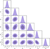 |
Fig. 1. MCMC contour plots of the Bézier interpolation. Darker (lighter) areas show the 1σ (2σ) confidence regions. |
Best-fit parameters with 1σ (2σ) error bars obtained from the MCMC analysis based on the Bézier interpolation of this work, compared to the flat and nonflat ΛCDM best-fit parameters (Planck Collaboration VI 2020).
These results show that our interpolation technique of intermediate-redshift data sets is able to set precise model-independent constraints on the key cosmological parameters ωb, ωm, h0, and Ωk listed in Table 4. It is immediately clear that these cosmic bounds agree within 1σ (2σ) with those obtained from the flat (nonflat) concordance model, but the attached errors are larger. In particular, the Hubble constant tension still remains unsolved because our value of h0 listed in Table 4 is still consistent at the 1σ confidence level with the value obtained from the CMB data (h0 = 0.6736 ± 0.0054) (Planck Collaboration VI 2020) and from SNe Ia (h0 = 0.7304 ± 0.0104) (Riess et al. 2022), both obtained in the flat scenario.
The constraint on Ωk of our work (see Table 4) is due to the scattered and limited redshift span (with respect to the other catalogs employed) of the galaxy cluster data (see the second panel in Fig. 2). This value is compatible at the 1σ level with the flat geometry reported by Planck (Planck Collaboration VI 2020). However, the large attached errors do not to exclude other geometries a priori, and for this reason, we compared our value of Ωk with the spatial curvature parameter listed in Table 5 of Planck Collaboration VI (2020), where the basic ΛCDM scenario is extended with a varying curvature parameter constrained by Planck TT, TE, and EE+lowE+lensing data. Moreover, when we compare our h0 with the reduced Hubble constant obtained from the above nonflat extension of the ΛCDM model (Planck Collaboration VI 2020), the consistency only reaches the 2σ level (see Table 4).
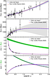 |
Fig. 2. Best-interpolating Bézier curves (blue curves) and 1σ confidence bands for H2(z), D2(z), δ2(z), and Δ2(z) (gray bands), and A2(z) and Θ2(z) (green bands), compared to the ΛCDM paradigm (Planck Collaboration VI 2020) (dashed red curves). |
4. Final outlooks and perspectives
We proposed a novel model-independent technique for extracting bounds on the key cosmological parameters, such as the normalized Hubble constant h0, the curvature parameter Ωk, and the matter densities ωb, for baryons, and ωm, for all the matter components.
To do this, we developed a calibration technique based on the well-established Bézier parametric curve and applied it to interpolate the OHD catalog with a second-order polynomial curve (Amati et al. 2019; Luongo & Muccino 2021b, 2023; Montiel et al. 2021; Muccino et al. 2023), without assuming any a priori cosmological models. Although no assumptions were made, by construction, the interpolating function, H2(z), carries out a valid constraint on α0 ≡ h0.
We then interpolated other intermediate-redshift catalogs that are based on galaxy cluster measurements and BAO data. Recently, SZ data have been used in conjunction with SNe Ia to infer cosmic bounds on H0 through the cosmic distance duality relation (Colaço et al. 2023). Here, we intentionally excluded SNe Ia (Scolnic et al. 2018) and CMB data (Planck Collaboration VI 2020), mainly because of the existing difference of the values of h0 obtained from these two sources.
Conversely, we used the Hubble rate H2(z) to obtain an interpolated angular diameter distance D2(z) that can be compared with galaxy cluster measurements. Since the interpolations H2(z) and D2(z) do not bear a priori assumptions on the spatial curvature, as long as the data sets do not carry specific priors on it, the galaxy cluster data provided model-independent bounds on Ωk.
In contrast to the procedure we developed in Luongo & Muccino (2023), where OHD and BAO catalogs were both interpolated by means of two different Bézier parametric curves, here we used four different data sets of BAO measurements and compared them with the interpolated function obtained by the combinations of the above-determined H2(z) and D2(z) with the aim to provide bounds on ωb and ωm and to reinforce the constraints on h0 and Ωk that were previously obtained from OHD and cluster data sets, respectively.
Specifically, the constraints on ωb and ωm were derived from the comoving sound horizon, rs, on which BAO data depend, and in general, ωb was fixed to the value obtained from the CMB. Because we did not employ CMB data, the degeneracy between ωb and ωm visible in Eq. (5) was bypassed by using the interpolated acoustic parameter, A2(z), for correlated BAO measurements (Blake et al. 2012).
The results provided by the MCMC analysis are based on the Metropolis algorithm and shown in Table 4 and Figs. 1 and 2. They show that our model-independent technique provides precise constraints, but with larger attached errors, on the key cosmological parameters. These constraints agree within the 2σ level with those obtained from the nonflat extension of the concordance model and agree better within 1σ also with h0 obtained from the flat scenario of the ΛCDM model.
The h0 tension is still not fully addressed, even though OHD, galaxy clusters, and BAO provide narrow constraints (see Table 4). At the 1σ confidence level, our h0 appears to be more consistent with Planck estimates in the flat scenario (Planck Collaboration VI 2020), and it is barely consistent with SNe Ia, that is, h0 = 0.7304 ± 0.0104 (Riess et al. 2022).
Accordingly, it is worth mentioning that a recent estimate obtained from SNe Ia based on surface brightness fluctuations measurements, that is, h0 = 0.7050 ± 0.0237 (Khetan et al. 2021), not only agrees with our findings, but also appears to indicate that the Hubble constant may be in between the extreme values.
When compared to the basic extension of the ΛCDM scenario with a varying curvature parameter, our h0 finally is consistent within 2σ with the value provided by Planck (see Table 5 in Planck Collaboration VI 2020), as listed in Table 4.
Our overall outputs on the spatial curvature, see Table 4, are thus compatible at the 1σ level with the flat geometry set out by the ΛCDM model and with its nonflat extension (Planck Collaboration VI 2020). In this respect, although no difference with the concordance model manifestly arose, our bounds on Ωk cannot exclude nonflat geometries a priori. They are only likely less probable than in the flat case. This loose constraint is mainly due to the scattered and limited redshift span of the galaxy cluster data, as shown in the second panel of Fig. 2.
We conclude that our model-independent method provides accurate constraints that confirm the ΛCDM background. Hence, neither small extensions of the standard cosmological model (Izzo et al. 2012; Muccino et al. 2021; Luongo et al. 2022) nor additional terms in the Hilbert-Einstein action (Capozziello et al. 2019) seem to be required.
To further refine our constraints, it would be crucial in the future to increase and improve the quality of the catalogs involved in this analysis. In particular,
-
High-redshift clusters are essential to minimize the uncertainty on Ωk with our technique, and
-
Increasing the number of correlated BAO measurements is certainly important to improve the constraints on ωb and ωm.
Finally, we remark that our technique can be used to calibrate gamma-ray bursts (Luongo & Muccino 2021a) and quasar (Risaliti & Lusso 2019) correlations in a model-independent way, as proposed in Luongo & Muccino (2023), strengthening the constraints and pushing our analysis further to z ∼ 9. Thus, our future efforts will be to explore new intermediate data catalogs with our method.
Acknowledgments
The work of OL and MM is partially supported by the Ministry of Education and Science of the Republic of Kazakhstan, Grant IRN AP08052311.
References
- Abbott, T. M. C., Abdalla, F. B., Alarcon, A., et al. 2019, MNRAS, 483, 4866 [NASA ADS] [CrossRef] [Google Scholar]
- Abdalla, E., Abellán, G. F., Aboubrahim, A., et al. 2022, J. High Energy Astrophys., 34, 49 [NASA ADS] [CrossRef] [Google Scholar]
- Aizpuru, A., Arjona, R., & Nesseris, S. 2021, Phys. Rev. D, 104, 043521 [CrossRef] [Google Scholar]
- Alam, S., Ata, M., Bailey, S., et al. 2017, MNRAS, 470, 2617 [Google Scholar]
- Amati, L., D’Agostino, R., Luongo, O., Muccino, M., & Tantalo, M. 2019, MNRAS, 486, L46 [CrossRef] [Google Scholar]
- Anderson, L., Aubourg, É., Bailey, S., et al. 2014, MNRAS, 441, 24 [Google Scholar]
- Arjona, R., Cardona, W., & Nesseris, S. 2019, Phys. Rev. D, 99, 043516 [NASA ADS] [CrossRef] [Google Scholar]
- Ata, M., Baumgarten, F., Bautista, J., et al. 2018, MNRAS, 473, 4773 [NASA ADS] [CrossRef] [Google Scholar]
- Aubourg, É., Bailey, S., Bautista, J. E., et al. 2015, Phys. Rev. D, 92, 123516 [Google Scholar]
- Bautista, J. E., Vargas-Magaña, M., Dawson, K. S., et al. 2018, ApJ, 863, 110 [NASA ADS] [CrossRef] [Google Scholar]
- Belfiglio, A., Giambò, R., & Luongo, O. 2022, arXiv e-prints [arXiv:2206.14158] [Google Scholar]
- Bernal, J. L., & Libanore, S. 2023, Cosmic Tensions - Lecture Notes [Google Scholar]
- Beutler, F., Blake, C., Colless, M., et al. 2011, MNRAS, 416, 3017 [NASA ADS] [CrossRef] [Google Scholar]
- Blake, C., Brough, S., Colless, M., et al. 2012, MNRAS, 425, 405 [Google Scholar]
- Bocquet, S., & Carter, F. W. 2016, J. Open Source Software, 1, 46 [NASA ADS] [CrossRef] [Google Scholar]
- Bonamente, M., Joy, M. K., LaRoque, S. J., et al. 2006, ApJ, 647, 25 [NASA ADS] [CrossRef] [Google Scholar]
- Borghi, N., Moresco, M., & Cimatti, A. 2022, ApJ, 928, L4 [NASA ADS] [CrossRef] [Google Scholar]
- Boshkayev, K., D’Agostino, R., & Luongo, O. 2019, Eur. Phys. J. C, 79, 332 [NASA ADS] [CrossRef] [Google Scholar]
- Capozziello, S., De Laurentis, M., Luongo, O., & Ruggeri, A. 2013, Galaxies, 1, 216 [NASA ADS] [CrossRef] [Google Scholar]
- Capozziello, S., D’Agostino, R., & Luongo, O. 2019, Int. J. Mod. Phys. D, 28, 1930016 [NASA ADS] [CrossRef] [Google Scholar]
- Carlstrom, J. E., Holder, G. P., & Reese, E. D. 2002, ARA&A, 40, 643 [Google Scholar]
- Carroll, S. M. 2001, Liv. Rev. Rel., 4, 1 [NASA ADS] [CrossRef] [Google Scholar]
- Colaço, L. R., Ferreira, M. S., Holanda, R. F. L., Gonzalez, J. E., & Nunes, R. C. 2023, arXiv e-prints [arXiv:2310.18711] [Google Scholar]
- Copeland, E. J., Sami, M., & Tsujikawa, S. 2006, Int. J. Mod. Phys. D, 15, 1753 [NASA ADS] [CrossRef] [Google Scholar]
- Cuceu, A., Farr, J., Lemos, P., & Font-Ribera, A. 2019, JCAP, 2019, 044 [Google Scholar]
- D’Agostino, R., Luongo, O., & Muccino, M. 2022, CQG, 39, 195014 [CrossRef] [Google Scholar]
- De Filippis, E., Sereno, M., Bautz, M. W., & Longo, G. 2005, ApJ, 625, 108 [NASA ADS] [CrossRef] [Google Scholar]
- Di Valentino, E., Mena, O., Pan, S., et al. 2021, CQG, 38, 153001 [NASA ADS] [CrossRef] [Google Scholar]
- du Mas des Bourboux, H., Rich, J., Font-Ribera, A., et al. 2020, ApJ, 901, 153 [CrossRef] [Google Scholar]
- Dunsby, P. K. S., & Luongo, O. 2016, Int. J. Geom. Methods Mod. Phys., 13, 1630002 [Google Scholar]
- Efstathiou, G., & Bond, J. R. 1999, MNRAS, 304, 75 [NASA ADS] [CrossRef] [Google Scholar]
- Glanville, A., Howlett, C., & Davis, T. M. 2021, MNRAS, 503, 3510 [NASA ADS] [CrossRef] [Google Scholar]
- Haridasu, B. S., Luković, V. V., Moresco, M., & Vittorio, N. 2018, JCAP, 2018, 015 [CrossRef] [Google Scholar]
- Hastings, W. K. 1970, Biometrika, 57, 97 [Google Scholar]
- Hou, J., Sánchez, A. G., Ross, A. J., et al. 2021, MNRAS, 500, 1201 [Google Scholar]
- Izzo, L., Luongo, O., & Capozziello, S. 2012, Mem. Soc. Astron. Ital. Suppl., 19, 37 [Google Scholar]
- Jiao, K., Borghi, N., Moresco, M., & Zhang, T.-J. 2023, ApJS, 265, 48 [NASA ADS] [CrossRef] [Google Scholar]
- Jimenez, R., & Loeb, A. 2002, ApJ, 573, 37 [NASA ADS] [CrossRef] [Google Scholar]
- Khetan, N., Izzo, L., Branchesi, M., et al. 2021, A&A, 647, A72 [NASA ADS] [CrossRef] [EDP Sciences] [Google Scholar]
- Li, E.-K., Du, M., & Xu, L. 2020, MNRAS, 491, 4960 [NASA ADS] [CrossRef] [Google Scholar]
- Liu, T., Cao, S., Li, X., et al. 2022, A&A, 668, A51 [NASA ADS] [CrossRef] [EDP Sciences] [Google Scholar]
- Luongo, O., & Muccino, M. 2018, Phys. Rev. D, 98, 103520 [CrossRef] [Google Scholar]
- Luongo, O., & Muccino, M. 2021a, Galaxies, 9, 77 [NASA ADS] [CrossRef] [Google Scholar]
- Luongo, O., & Muccino, M. 2021b, MNRAS, 503, 4581 [NASA ADS] [CrossRef] [Google Scholar]
- Luongo, O., & Muccino, M. 2023, MNRAS, 518, 2247 [Google Scholar]
- Luongo, O., Muccino, M., Colgáin, E. O., et al. 2022, Phys. Rev. D, 105, 103510 [NASA ADS] [CrossRef] [Google Scholar]
- Metropolis, N., Rosenbluth, A. W., Rosenbluth, M. N., Teller, A. H., & Teller, E. 1953, J. Chem. Phys., 21, 1087 [Google Scholar]
- Montiel, A., Cabrera, J. I., & Hidalgo, J. C. 2021, MNRAS, 501, 3515 [Google Scholar]
- Moresco, M. 2015, MNRAS, 450, L16 [NASA ADS] [CrossRef] [Google Scholar]
- Moresco, M., Cimatti, A., Jimenez, R., et al. 2012, JCAP, 2012, 006 [CrossRef] [Google Scholar]
- Moresco, M., Pozzetti, L., Cimatti, A., et al. 2016, JCAP, 2016, 014 [CrossRef] [Google Scholar]
- Moresco, M., Amati, L., Amendola, L., et al. 2022, Liv. Rev. Rel., 25, 6 [NASA ADS] [CrossRef] [Google Scholar]
- Muccino, M., Izzo, L., Luongo, O., et al. 2021, ApJ, 908, 181 [Google Scholar]
- Muccino, M., Luongo, O., & Jain, D. 2023, MNRAS, 523, 4938 [NASA ADS] [CrossRef] [Google Scholar]
- Padmanabhan, N., Xu, X., Eisenstein, D. J., et al. 2012, MNRAS, 427, 2132 [Google Scholar]
- Percival, W. J., Reid, B. A., Eisenstein, D. J., et al. 2010, MNRAS, 401, 2148 [Google Scholar]
- Perlmutter, S., Aldering, G., Goldhaber, G., et al. 1999, ApJ, 517, 565 [Google Scholar]
- Planck Collaboration VI. 2020, A&A, 641, A6 [NASA ADS] [CrossRef] [EDP Sciences] [Google Scholar]
- Ratsimbazafy, A. L., Loubser, S. I., Crawford, S. M., et al. 2017, MNRAS, 467, 3239 [NASA ADS] [CrossRef] [Google Scholar]
- Riess, A. G., Filippenko, A. V., Challis, P., et al. 1998, AJ, 116, 1009 [Google Scholar]
- Riess, A. G., Yuan, W., Macri, L. M., et al. 2022, ApJ, 934, L7 [NASA ADS] [CrossRef] [Google Scholar]
- Risaliti, G., & Lusso, E. 2019, Nat. Astron., 3, 272 [Google Scholar]
- Ross, A. J., Samushia, L., Howlett, C., et al. 2015, MNRAS, 449, 835 [NASA ADS] [CrossRef] [Google Scholar]
- Sahni, V., & Starobinsky, A. 2000, Int. J. Mod. Phys. D, 9, 373 [Google Scholar]
- Scolnic, D. M., Jones, D. O., Rest, A., et al. 2018, ApJ, 859, 101 [NASA ADS] [CrossRef] [Google Scholar]
- Seo, H.-J., Ho, S., White, M., et al. 2012, ApJ, 761, 13 [NASA ADS] [CrossRef] [Google Scholar]
- Shafieloo, A. 2007, MNRAS, 380, 1573 [CrossRef] [Google Scholar]
- Shafieloo, A., & Clarkson, C. 2010, Phys. Rev. D, 81, 083537 [NASA ADS] [CrossRef] [Google Scholar]
- Simon, J., Verde, L., & Jimenez, R. 2005, Phys. Rev. D, 71, 123001 [NASA ADS] [CrossRef] [Google Scholar]
- Sridhar, S., Song, Y.-S., Ross, A. J., et al. 2020, ApJ, 904, 69 [NASA ADS] [CrossRef] [Google Scholar]
- Stern, D., Jimenez, R., Verde, L., Kamionkowski, M., & Stanford, S. A. 2010, JCAP, 2010, 008 [Google Scholar]
- Sunyaev, R. A., & Zeldovich, Y. B. 1970, Comm. Astrophys. Space Phys., 2, 66 [Google Scholar]
- Sunyaev, R. A., & Zeldovich, Y. B. 1972, Comm. Astrophys. Space Phys., 4, 173 [Google Scholar]
- Tsujikawa, S. 2011, in Astrophysics and Space Science Librar, eds. S. Matarrese, M. Colpi, V. Gorini, & U. Moschella, Astrophys. Space Sci. Lib., 370, 331 [NASA ADS] [CrossRef] [Google Scholar]
- Weinberg, S. 2008, Cosmology (New York: Oxford University Press) [Google Scholar]
- Zhang, C., Zhang, H., Yuan, S., et al. 2014, Res. Astron. Astrophys., 14, 1221 [CrossRef] [Google Scholar]
- Zhang, K., Zhou, T., Xu, B., Huang, Q., & Yuan, Y. 2023, ApJ, 957, 5 [NASA ADS] [CrossRef] [Google Scholar]
All Tables
Redshift distribution (first column) of the OHD measurements with the statistical errors (second column) and the reference papers (third column).
Sample of galaxy clusters with redshift (first column) and diameter angular distances (second column), taken from De Filippis et al. (2005).
Four BAO catalogs with surveys (first column), redshifts (second column), measurements with errors (third column), and references (fourth column).
Best-fit parameters with 1σ (2σ) error bars obtained from the MCMC analysis based on the Bézier interpolation of this work, compared to the flat and nonflat ΛCDM best-fit parameters (Planck Collaboration VI 2020).
All Figures
|
Fig. 1. MCMC contour plots of the Bézier interpolation. Darker (lighter) areas show the 1σ (2σ) confidence regions. |
| In the text | |
|
Fig. 2. Best-interpolating Bézier curves (blue curves) and 1σ confidence bands for H2(z), D2(z), δ2(z), and Δ2(z) (gray bands), and A2(z) and Θ2(z) (green bands), compared to the ΛCDM paradigm (Planck Collaboration VI 2020) (dashed red curves). |
| In the text | |
Current usage metrics show cumulative count of Article Views (full-text article views including HTML views, PDF and ePub downloads, according to the available data) and Abstracts Views on Vision4Press platform.
Data correspond to usage on the plateform after 2015. The current usage metrics is available 48-96 hours after online publication and is updated daily on week days.
Initial download of the metrics may take a while.